Particle-based non-Newtonian fluid animation for melting ... - PUC-Rio

Particle-based non-Newtonian fluid animation for melting objects
AFONSO PAIVA, FABIANO PETRONETTO, THOMAS LEWINER AND GEOVAN TAVARES
Department of Mathematics — Pontifícia Universidade Católica — Rio de Janeiro — Brazil
{apneto, fbipetro, tomlew, tavares}@mat.puc--rio.br.
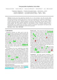
Abstract. This paper presents a new visually realistic animation technique for objects that melt and flow. It
simulates viscoplastic properties of materials such as metal, plastic, wax, polymer and lava. The technique consists
in modeling the object by the transition of a non–Newtonian fluid with high viscosity to a liquid of low viscosity.
During the melting, the viscosity is formulated using the General Newtonian fluids model, whose properties depend
on the local temperature. The phase transition is then driven by the heat equation. The fluid simulation framework
uses a variation of the Lagrangian method called Smoothed Particle Hydrodynamics. This paper also includes
several schemes that improve the efficiency and the numerical stability of the equations.
Keywords: Melting. Smoothed Particle Hydrodynamics. Non–Newtonian Fluid. Heat Equation. Physically
Based Animation. Computational Fluid Dynamics.
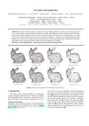
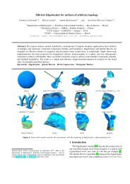
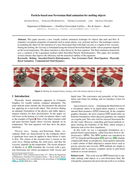
Figure 1: Melting the Stanford bunny starting cold at the bottom and hot at the top.
1 Introduction
Physically based animations appeared in Computer
Graphics for visually realistic computer animations. The
main delicate point remains the discretisation the physical
law applying on a real-world object. This involves finding
an adequate formulation of the physics and stable approximation
schemes for their discretisation. In this paper, we
will focus on the heating of a solid viscoplastic object, such
as the example of Figure 1. Parts of the object remains solid
and parts becomes liquid, whose viscosity depends on its
temperature. The heat equation will thus drive the phase
transition.
Physical laws. Among non-Newtonian fluids, viscoplastic
fluids are characterized by the toothpaste effect:
a significant force must be applied to them before it starts
to flow. The critical of the external force is known as the
yield stress. During melting, the yield stress, and thus the
viscosity, depends on the temperature. The recent advances
of Mendes et al. [12] formulate the viscosity with a general
Newtonian law which encompasses both viscous and
Preprint MAT. 15/06, communicated on May 14 th , 2006 to the Department
of Mathematics, Pontifícia Universidade Católica — Rio de Janeiro, Brazil.
The corresponding work was published in the proceedings of the Sibgrapi
2006, pp. 78–85. IEEE Press, 2006.
liquid state. The conciseness and generality of this formulation
suits better for melting, and we introduce it here for
simulation.
Approximation scheme. Simulating the fluid behavior of
a viscoplastic object in its liquid phase requires a computational
fluid dynamics (CFD) framework. In the computer
graphics literature, the most common CFD model relies on
Eulerian formulation where physical quantities are sampled
on a regular grid. This suits well for classical Newtonian fluids
like water. However, controlling grid based methods require
tracking the boundary of the fluid, which remains a
laborious task in free flow simulations.
In this work, we use a Lagrangian formulation on a
particle-based representation, called Smoothed Particle Hydrodynamics
(SPH). The SPH method was introduced in
1977 by Gingold and Monaghan [13] and Lucy [10] simulate
compressible fluids in astrophysics. Each particle represents
a small volume of fluid subjected to natural forces such as
gravity, pressure and viscosity. SPH methods are simple to
implement and its accuracy compares nicely to grid based
methods in several instances.
Related works This work uses the SPH framework to simulate
melting solid objects as a non–Newtonian fluid. We
will quickly summarize the most relevant work to us on these

A. Paiva, F. Petronetto, T. Lewiner and G. Tavares 2
three topics.
Smoothed Particle Hydrodynamics. The SPH method
was introduced in the computer graphics community by Desbrun
and Cani in [5], where they used SPH to simulate deformable
bodies. Müller et al. [19] then used the SPH approach
for simulating incompressible fluids with surface tension.
Furthermore, they introduced point–splatting to capture
the fluid free surface. Recently SPH methods became very
popular in the special effects industry where it was used to
simulate lava flow in the third part of The Lord of the Rings
trilogy (http://www.nextlimit.com).
Non–Newtonian fluids. There are few works in computer
graphics for non-Newtonian fluids. Goktekin et al. [6]
proposed a grid–based method to compute the stress tensor
of these fluids. They use a linear Maxwell model with
von Mises plastic yield condition. Clavet et al. [3] use SPH
with a linear combination of elastic springs between particles
driven plastic yield condition. Another method using SPH
was proposed by Mao and Yang [11], where the stress tensor
derives from a corotational Maxwell model.
Melting. The idea of simulating melting and flowing of
solids objects by coupling viscosity with temperature appeared
in different contexts. Carlson et al. [2] use an Eulerian
grid-based fluid method. They further need an implicit
integrator to compensate the instability of the grid–based approach.
Wei et al. [22] use cellular automata and replace
Navier–Stokes equations by simple rules in each automata.
Müller et al. [20] create a point–based framework to simulate
elastoplastic objects with von Mises plastic yield condition.
They use moving least squares (MLS) for approximating the
velocity gradient. Finally, Keiser et al. in [8] introduces traditional
SPH method in the previous framework with usual
viscoplastic modeling.
Contributions. This paper introduces two new elements to
the melting simulation. First, we use General Newtonian
Fluid model [12] to compute the viscosity (see Section 2).
Its concise formulation reduces the number of parameters for
yield modeling and allows simpler relation with the temperature.
Moreover, since this formulation covers viscoplastic
fluids within a single equation, it treats the whole object at
once and avoids delicate detection of the viscosity transition.
Moreover, we introduce in the heat equation approximation
a more stable Laplacian operator on the particles (see
Section 3). This approximation already improved Poisson
simulations [4] by involving differences of first derivatives
instead of second derivatives.
We also introduce several numerical improvements in the
method. First, we introduce the use of XSPH [14] for avoiding
the formation of stable clusters of particles (see Section
3). Then, we reintroduce the artificial viscosity [5], but
for melting simulation. We also chose the continuity equation
for density (equation (6)) to avoids particle outliers.
Finally, our implementation uses an adaptive time step for
each iteration based on the Courant-Friedrichs-Lewy condition
(see Section 4).
2 Formulation of the physical laws
Computational fluid dynamics (CFD) aims at prediction
fluid behavior through Navier–Stokes equations. These equations
are commonly solved using conventional Eulerian formulation
with grid-based methods such as finite differences
and finite elements. In this work, we chose an alternative
method driven by the Lagrangian formulation. As opposed
to the Eulerian approach, the Lagrangian formulation does
not require advective term, which suits well for meshless
methods such as SPH. We will introduce now this formulation
and the General Newtonian Fluid model [12] that models
our viscoplastic object, together with our heating model.
The reader will find further details on CFD in Anderson’s
book [1].
Lagrangian formulation. Navier-Stokes equations can be
formulated by the following two equations describing the
conservation of the mass (equation (1)) and of the momentum
(equation (2)).
dρ
= −ρ∇.v (1)
dt
dv
dt = − 1 ρ ∇p + 1 ∇.S + g (2)
ρ
where t denotes the time, v the velocity vector, ρ the density,
p the pressure, g the gravity acceleration vector and S the
viscoplastic stress tensor. This last term plays a fundamental
role in melting simulation.
Generalized Newtonian Fluid model. For non-Newtonian
fluids, the stress tensor is a nonlinear function of the deformation
tensor D = ∇v + (∇v) T . For our simulation, we
will use the Generalized Newtonian Liquid model proposed
by Mendes et al. [12], where the stress tensor S is given by
S = η (D) D, where the apparent
√
viscosity η depends on the
1
intensity of deformation D =
2 · trace (D)2 . The viscosity
function η is then given by:
(
η (D) = (1 − exp [− (J + 1) D]) D n−1 + 1 )
(3)
D
where n is the behavior of power–law index and J is the
jump number.
The jump number J is a new rheological parameter of a
viscoplastic fluid which combines previous ones such as the
yield stress and the consistency index. In our simulation, we
fixed n = 1 2
, and let only the jump number J vary with the
temperature.
Heating and melting. The melting of volumetric objects
corresponds to a phase transition from solid to fluid. We
can model this transition by varying the viscosity according
to the temperature of each particle. This model was used
in other animation frameworks, either using grid-based approach
[2] or particle-based approach [8].
The time variation of the temperature is described by the
The corresponding work was published in the proceedings of the Sibgrapi 2006, pp. 78–85. IEEE Press, 2006.

3 Particle-based non-Newtonian fluid animation for melting objects
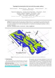
(a) Initial temperature. (b) 500 iterations. (c) 1060 iterations. (d) 3000 iterations.
Figure 2: Temperature of the 9727 particles of the bunny of Figure 1: the dark blue parts are below the melting point, and thus remain solid.
Observe that the left ear of the bunny gets colder after touching the body.
following heat equation, involving the temperature T and the
thermal diffusion constant k:
dT
dt = k∇2 T (4)
When the temperature of some part of the object increases
and reaches the melting point, it becomes liquid (see Figure
2). The jump number J then decreases according to the
temperature. We will model the jump number as decreasing
linearly with respect to the temperature:
J (T ) = (1 − u)J max − uJ min
with u = (T −T min )/(T max −T min ). Note that the viscosity
function of equation (3) thus decreases when temperature
increases and vice-versa.
3 Particle–based approximation scheme
We will use here the Smoothed Particle Hydrodynamics
(SPH) framework for simulating the fluid behavior. In our
animation framework, we use the formulation of SPH for
incompressible fluid [15]. A wide review of SPH methods
can be found in Monaghan’s survey [17].
The SPH principles are reviewed in section 3(a) Smoothed
Particle Hydrodynamics. It requires a discretisation of the different
terms of the governing equations: section 3(b) Particle
approximation of continuity describes the approximation of the
density for the continuity equation (1), section 3(c) Particle
approximation of the momentum describes the approximation of
the pressure and the stress tensor of the momentum equation
(2). Sections 3(d) and 3(e) present corrections for the
viscosity and the velocity. Finally, section 3(f) Laplacian approximation
introduces our approximation of the Laplacian in
the heat equation (4).
(a) Smoothed Particle Hydrodynamics
The key idea of SPH is to replace the fluid by a set
of particles (see Figure 3). The dynamics of the fluid is
then naturally governed by the Lagrangian version of the
Navier-Stokes equations introduced in the last Section. The
local fluid properties such as mass and volume are attached
to each particle and interpolated in-between particles. This
interpolation uses a smoothing kernel W on the particles in
a radius of h. A scalar field A(x) and its associated gradient
vector field ∇A(x) at point x are interpolated using the
particles j within a disk of radius h around x as follows:
A(x) =
∇A(x) =
n∑
A(x j ) m j
W (x − x j , h) (5)
ρ j
j=i
n∑
A(x j ) m j
∇W (x − x j , h)
ρ j
j=i
where n is the number of neighboring particles, j the particle
index, x j the particle position, m j the particle mass and ρ j
the particle density.
Figure 4: Quintic smoothing kernel: the particles farther than the
smoothing length h are not considered in the convolution.
In this work, we choose a piecewise quintic smoothing
kernel function (see Figure 4), ( )
W (x−x j , h) = 3
359 πh3 ‖x−xj ‖ · w
h
, with:
⎧
(3−q) ⎪⎨
5 −6(2−q) 5 + 15(1−q) 5 ; 0 ≤ q < 1
(3−q)
w(q) =
5 −6(2−q) 5 ; 1 ≤ q < 2
(3−q) ⎪⎩
5 ; 2 ≤ q ≤ 3
0 ; q > 3
Preprint MAT. 15/06, communicated on May 14 th , 2006 to the Department of Mathematics, Pontifícia Universidade Católica — Rio de Janeiro, Brazil.

A. Paiva, F. Petronetto, T. Lewiner and G. Tavares 4
Figure 3: SPH schemes deal gracefully with complex topological of the chair surface.
(b) Particle approximation of continuity
Density is usually approximate in SPH systems using the
density summation, which follows directly from the SPH
approximation of equation (5):
ρ i =
n∑
m j W (x i − x j , h)
j=i
However, to ensure the physical meaning of the approximation,
we need to introduce a symmetrization between the
pressure and the local velocity [9]. In particular, the density
summation approach has a particle deficiency near the
fluid interface, which leads to spurious results. Moreover, it
requires more computational efforts since the density must
be evaluated before other parameters, such as pressure. We
therefore chose another approximation for the density, using
the following SPH version of continuity equation (1):
dρ i
dt = ρ i
n∑
j=1
m j
ρ j
(v i − v j ) .∇ i W (x ij , h) . (6)
where v i and v j are velocities at particles i and j respectively,
and x ij = x i − x j .
(c) Particle approximation of the momentum
Pressure. The modeling of pressure remains a delicate
point for SPH simulations of incompressible fluids, due
to the lack of explicit control of the local density. Since
SPH suits better for compressible fluid, we approximate the
incompressible fluid by a quasi-compressible fluid through
an equation of state [15] for the pressure. We use the one
proposed by Morris et al. [18]:
p i = c 2 (ρ i − ρ 0 ) (7)
where p i is the pressure at particle i, c the speed of sound,
which represents the fastest velocity of a wave propagation
in that medium, and ρ 0 is a reference density. This equation
of state is very similar with the ideal gas equation of state
used by Desbrun and Cani [5].
After updating the pressure at all particles using equation
(7), we can evaluate the pressure term in equation (2)
at each particle i using a symmetrization similar to the density
case [9]:
− 1 ρ i
∇p i = −
n∑
j=1
m j
(
p i
ρ 2 i
+ p j
ρ 2 j
)
∇ i W (x ij , h).
Stress tensor. In order to compute the stress tensor S i =
η (D i ) D i at each particle i, where η (D i ) is given by the
equation (3), we must pre-compute the deformation tensor:
D i = ∇v i + (∇v i ) T
where the velocity is evaluated by the following equation:
∇v i =
n∑
j=1
m j
ρ j
(v j − v i ) ⊗ ∇ i W (x ij , h) .
Finally, after updating of the stress tensor S i at each
particle i, the stress term in equation (2) can be approximated
by:
1
ρ i
∇.S i =
n∑
j=1
m j
(d) Viscosity correction
ρ i ρ j
(S i + S j ) .∇ i W (x ij , h) .
To avoid numerical instabilities due to oscillations in the
velocity vector field, which may ruin the simulation, a common
technique adds an artificial viscous stress term in the
SPH approximation of the linear momentum (equation (2))
as follows:
dv i
dt ← dv i
dt − n ∑
j=1
m j
ρ i
∏
ij ∇ iW (x ij , h) . (8)
The effect of the artificial viscous stress is given by the
term:
and
⎧
⎪⎨ −αµ ij c+βµ 2 ij
∏
ij = 0.5(ρ i +ρ j )
, (v i − v j ) .(x i − x j ) < 0
⎪ ⎩
0, (v i − v j ) .(x i − x j ) ≥ 0
µ ij = h (v i − v j ) .(x i − x j )
|x i − x j | 2 + 0.01h 2
where α corresponds to bulk viscosity and β corresponds to
von Neumann-Ritchmyer viscosity [17].
The corresponding work was published in the proceedings of the Sibgrapi 2006, pp. 78–85. IEEE Press, 2006.

5 Particle-based non-Newtonian fluid animation for melting objects
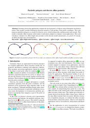
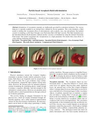
(a) 20 iterations. (b) 550 iterations. (c) 780 iterations. (d) 1320 iterations.
Figure 5: Melting a completely liquid Gargoyle model using 6976 particles: the color codes the velocity of each particle. The stability of the
method preserves the shape of the object without explicit mesh representation even after many iterations.
(e) XSPH Velocity correction
Algorithm 1 Particle dynamics
1: repeat
To prevent particle inter–penetration, which may result
2: for each particle i do
in stable clusters of particles, Monaghan [14] introduced
3: Update derivative density (equation 6)
an improvement called XSPH velocity-correction. In XSPH
4: Update acceleration (equation 2)
(X means unknown), each particle i moves in the following
5: Correct acceleration (equation 8)
way:
6: Update derivative temperature (equation 4)
7: end for
n∑ m j
v i ← v i + ε
0.5 (ρ
j=1 i + ρ j ) (v 8: for each particle i do
j − v i ) W (x ij , h) (9)
9: Update x i , v i , T i and ρ i with Leap-Frog scheme
10: Correct v i with XSPH (equation 9)
where ε ∈ [0, 1].
11: Update p i (equation 7)
The XSPH technique consists in computing an average 12: Update viscosity (equation 3)
velocity from the velocities of the neighboring particles, it 13: end for
helps to keep particles of an incompressible flow to move 14: Update particle neighbors
more orderly.
15: Update △t using CFL condition (equation 10)
16: time = time + △t
(f) Laplacian approximation
17: until time < time total
The Heat equation (4), which governs the phase transition
from solid to fluid, requires an approximation for the Laplacian
of the temperature ∇ 2 T i . This second derivative can be 4 Results and Implementation
approximated using the normal SPH convolution by the use
In implementing a particle system we have two descriptions
a global one and local one. The local description takes
of second derivatives for each particle i [8]:
care of a single particle entity and of the attribute stored at
n∑
∇ 2 m j
T i = (T i − T j ) ∇ 2 i W (x ij , h) .
each particle. In our model there are system attributes and
ρ
j=1 j particle attributes. The particle system attributes like mass,
speed of sound and the smoothing length h are global and
However, the above equation has some disadvantages they do not change with respect to time. The particle attributes
vary with respect to time thus they must be stored
such as sensibility to particle disorder: the heat transfer between
particles may be positive or negative since the second at each particle, these attributes are given by table 1. These
derivatives can change sign. The heat equation using this approximation
may not conserve the thermal energy in the adi-
attributes are updated in the sequence of algorithm 1.
(a) Numerical integration
abatic enclosure [16].
For these reasons, we use a Laplacian operator involving The SPH fluid equations are integrated with the second
only first derivatives, which was first proposed by Cummins order accurate Leap-Frog scheme [9]. The advantages of
and Rudman [4] to solve the Poisson equation with the SPH Leap-Frog algorithm are computational efficiency for one
version of the Projection Method. Its expression follows: fluid equation evaluation per step and the low memory storage
required in the evaluation. The stability in this explicit
n∑
( )
∇ 2 m j 4ρi
T I =
(T i − T j ) x ij.∇ i W (x ij , h) time integration scheme is due to the Courant-Friedrichsρ
j=1 j ρ i + ρ j |x ij | 2 + 0.01h . Lewy (CFL) condition, where adaptive time step is given by
2
{
h
△t = 0.1 min
|v max | + c 2 , h 2 }
. (10)
6 η max
Preprint MAT. 15/06, communicated on May 14 th , 2006 to the Department of Mathematics, Pontifícia Universidade Católica — Rio de Janeiro, Brazil.

A. Paiva, F. Petronetto, T. Lewiner and G. Tavares 6
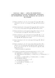
(a) Initial object.
(b) 390 iterations.
(c) 800 iterations.
(d) 2000 iterations.
Figure 6: Melting of the SIBGRAPI logo using 12900 particles, starting cold at the bottom and hot at the top. The adaptive time step allows
an accurate simulation with few iterations.
Attribute Description
x
position
v
velocity
a
acceleration
D
deformation tensor
ρ
density
η
viscosity
T
temperature
Table 1: Particle attributes.
This adaptive time step allows reducing the number of iteration
while maintaining accuracy (see Figure 6).
(b) Neighbors retrieval
In contrast with grid-base methods, where the positions
of neighboring grid-cells are well defined, the neighbors of
a given particle in the SPH method can vary with time.
An adaptive hierarchy tree search [7] is adopted to find the
particle neighbors.
The tree search method splits recursively the problem
domain into octants that contain particles, until the leaves
on the tree has a maximum particle number (we use at most
ten particles for each leaf). After the tree structure is built,
the search process can be performed.
For a given particle i, a cube with side 6h centered at
x i is used to enclose the particle. We check at each level
of the tree if the cube intersects the tree nodes containing
the particles. If they do not intersect we stop the descent
down on that particular path. If they do intersect we go to
The corresponding work was published in the proceedings of the Sibgrapi 2006, pp. 78–85. IEEE Press, 2006.

7 Particle-based non-Newtonian fluid animation for melting objects
the next level and repeat the process until we reach the tree
leaves containing particles. Now we check if each particle is
inside of the support domain of the current particle i. If it is
we record it as a particle neighbor. The complexity of this
tree search method is of order O(n log(n)), n being the total
particle number.
(c) Rendering
The tracking of the fluid free surface is done by rendering
an isosurface from the SPH approximation of its characteristic
function:
χ (x) =
n∑
j=1
m j
ρ j
W (x − x j , h)
where the isovalue is in the range [0, 1].
We use an efficient and robust implementation of the
marching cubes algorithm [21] to generate the triangle mesh
for the isosurface. To improve the evaluation at the grid
nodes we use the same hierarchical data structure for search
neighboring particles.
The animations of Figures. 1 and 6 were rendered using
the open–source ray tracer POV–Ray (http://www.
povray.org).
(d) Results
We tested the method described in this paper on simple
models. The example of Figures. 1 and 2 simulates the melting
of the Stanford bunny with 9727 particles. The simulation
is initialized with a linear gradient of temperature such
that the ears melt while the body remains cold and solid. The
visual result of Figure 1 matches the intuition of the process.
Moreover, the physical behavior is coherent, especially since
one of the ears gets colder when touching the body, while the
other one remains hot (see Figure 2).
In this work, we combined many advanced discretisation
schemes to guarantee the stability of the simulation. The
SPHmethod already offers simple handling of topological
singularities, as for the 10000 particles simulation of Figure
3. This efforts result impressively when simulating the
only flowing part of the melting, as on Figure 5. In that case,
all the 6976 particles start above the melting point, and flows
as a non–Newtonian fluid. The good handling of viscosity in
SPH techniques allows very realistic results. For example,
the head of the gargoyle remains well defined even when almost
completely melted.
Finally, the proposed adaptive time step allows efficient
simulations. For example, the melting of the Sibgrapi logo
of Figure 6 used 12900 particles, i.e. more particles than for
the bunny. However, it required less execution time for the
simulation (see Table 2). This is due to the lower density of
the model, which allowed bigger time steps.
5 Conclusions and future works
This paper proposed a physical simulation for melting
viscoplastic objects. Our simulation relies on the SPH
framework, and implements the General Newtonian Fluid
model for viscoplastic fluids. It is further enhanced in numerical
stability by adapted discretisation of the Navier–Stokes
equation terms, and by a stable Laplacian operator for the
heat equation. The effectiveness of the method is illustrated
on simple examples which match the physical laws, leading
to an efficient scheme for both animation and simulation purposes.
This work can be improved mainly in two directions. On
one side, the inner nature of SPH systems permits a straightforward
parallelization of the algorithm, which would increase
the possible number of particles used during the simulation.
On the other side, the rendering remains a fundamental
part for animation purposes. The isosurfacing approach
may be complemented by advanced rendering techniques
during the simulation, in order to produce the final animation
directly.
Animation Number of Time per
particles iteration
Bunny 9727 0.94s
Chair 10000 0.75s
Gargoyle 6976 1.06s
Sibgrapi 12900 0.92s
Table 2: Average timings of the example animations running on
Pentium 4 – 2.4 GHz. Note that in the Gargoyle simulation, all
particles were fluids.
Acknowledgments
We would like to thank Prof. Paulo Roberto Mendes (Department
of Mechanical Engineering, PUC–Rio) for suggesting
us to use his viscoplastic fluid model. The authors are
members of Matmidia laboratory at PUC–Rio which is sponsored
by CNPq, FAPERJ and Petrobras.
References
[1] J. D. Anderson. Computational Fluid Dynamics.
McGraw-Hill, 1995.
[2] M. Carlson, P. Mucha, B. Van Horn III and G. Turk.
Melting and flowing. In Symposium on Computer Animation,
pages 167–174, 2002.
[3] S. Clavet, P. Beaudoin and P. Poulin. Particle-based viscoelastic
simulation. Symposium on Computer Animation,
pages 219–228, 2005.
Preprint MAT. 15/06, communicated on May 14 th , 2006 to the Department of Mathematics, Pontifícia Universidade Católica — Rio de Janeiro, Brazil.

A. Paiva, F. Petronetto, T. Lewiner and G. Tavares 8
[4] S. J. Cummins and M. Rudman. An sph projection
method. Journal of Computational Physics, 152:584–
607, 1999.
[5] M. Desbrun and M. P. Cani. Smoothed particles: A
new paradigm for animating highly deformable bodies.
In Computer Animation and Simulation ’96, pages 61–
76. Animation and Simulation, Springer-Verlag, August
1996.
[6] T. G. Goktekin, A. W. Bargteil and J. F. O’Brien. A
method for animating viscoelastic fluids. ACM Transactions
on Graphics, 23(3):463–468, 2004.
[7] L. Hernquist and N. Katz. Treesph: A unification of SPH
with hierarchical tree method. The Astrophysical Journal
of Supplement Series, 70:419–446, 1989.
[19] M. Müller, D. Charypar and M. Gross. Particle-based
fluid simulation for interactive applications. In Symposium
on Computer Animation, pages 154–159, 2003.
[20] M. Muller, R. Keisser, A. Nealen, M. Pauly, M. Gross
and M. Alexa. Point based animation of elastic, plastic
and melting. Symposium on Computer Animation, pages
141–151, 2004.
[21] T. Lewiner, H. Lopes, A. W. Vieira and G. Tavares.
Efficient implementation of marching cubes’ cases with
topological guarantees. Journal of Graphics Tools,
8(2):234–241, 2003.
[22] X. Wei, W. Li and A. Kaufman. Melting and flowing of
viscous volumes. Computer Animation and Social Agents,
pages 54–59, 2003.
[8] R. Keiser, B. Adams, D. Gasser, P. Bazzi, P. Dutré and
M. Gross. A unified lagrangian approach to solid-fluid animation.
In Proceedings of the Eurographics Symposium
on Point-Based Graphics, pages 125–134, 2005.
[9] S. Li and W. K. Liu. Meshfree Particle Methods.
Springer, 2004.
[10] L. B. Lucy. Numerical approach to testing the fission
hyphotesis. Astronomical Journal, 82:1013–1024, 1977.
[11] H. Mao and Y. Yang. A particle-based model for nonnewtonian
fluid. Technical Report TR05-05, University
of Alberta, 2005.
[12] P. R. S. Mendes, E. S. S. Dutra, J. R. R. Siffert and
M. F. Naccache. Gas displacement of viscoplastic liquids
in cappilary tubes. Journal of Non-Newtonian Fluid Mechanics,
2005. (to appear).
[13] R. A. Gingold and J. J. Monaghan. Smoothed particle
hydrodynamics: theory and application to non-spherical
stars. Monthly Notices of the Royal Astronomical Society,
181:375–389, 1977.
[14] J. J. Monaghan. On the problem of penetration in
particle methods. Journal of Computational Physics,
82:1–15, 1989.
[15] J. J. Monaghan. Simulating free surface flow with SPH.
Journal of Computational Physics, 110:399–406, 1994.
[16] P. W. Cleary and J. J. Monaghan. Conduction modelling
using smoothed particle hydrodynamics. Journal
of Computational Physics, 148:227–264, 1999.
[17] J. J. Monaghan. Smoothed particle hydrodynamics.
Reports on Progress in Physics, 68:1703–1759, 2005.
[18] J. P. Morris, P. J. Fox and Y. Zhu. Modeling low
Reynolds number for incompressible flows using SPH.
Journal of Computational Physics, 136:214–226, 1997.
The corresponding work was published in the proceedings of the Sibgrapi 2006, pp. 78–85. IEEE Press, 2006.