Particle-based non-Newtonian fluid animation for melting ... - PUC-Rio

A. Paiva, F. Petronetto, T. Lewiner and G. Tavares 4
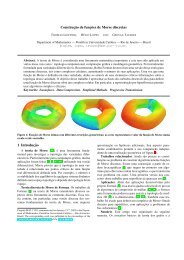
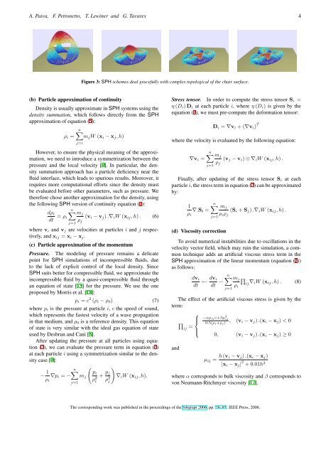
Figure 3: SPH schemes deal gracefully with complex topological of the chair surface.
(b) Particle approximation of continuity
Density is usually approximate in SPH systems using the
density summation, which follows directly from the SPH
approximation of equation (5):
ρ i =
n∑
m j W (x i − x j , h)
j=i
However, to ensure the physical meaning of the approximation,
we need to introduce a symmetrization between the
pressure and the local velocity [9]. In particular, the density
summation approach has a particle deficiency near the
fluid interface, which leads to spurious results. Moreover, it
requires more computational efforts since the density must
be evaluated before other parameters, such as pressure. We
therefore chose another approximation for the density, using
the following SPH version of continuity equation (1):
dρ i
dt = ρ i
n∑
j=1
m j
ρ j
(v i − v j ) .∇ i W (x ij , h) . (6)
where v i and v j are velocities at particles i and j respectively,
and x ij = x i − x j .
(c) Particle approximation of the momentum
Pressure. The modeling of pressure remains a delicate
point for SPH simulations of incompressible fluids, due
to the lack of explicit control of the local density. Since
SPH suits better for compressible fluid, we approximate the
incompressible fluid by a quasi-compressible fluid through
an equation of state [15] for the pressure. We use the one
proposed by Morris et al. [18]:
p i = c 2 (ρ i − ρ 0 ) (7)
where p i is the pressure at particle i, c the speed of sound,
which represents the fastest velocity of a wave propagation
in that medium, and ρ 0 is a reference density. This equation
of state is very similar with the ideal gas equation of state
used by Desbrun and Cani [5].
After updating the pressure at all particles using equation
(7), we can evaluate the pressure term in equation (2)
at each particle i using a symmetrization similar to the density
case [9]:
− 1 ρ i
∇p i = −
n∑
j=1
m j
(
p i
ρ 2 i
+ p j
ρ 2 j
)
∇ i W (x ij , h).
Stress tensor. In order to compute the stress tensor S i =
η (D i ) D i at each particle i, where η (D i ) is given by the
equation (3), we must pre-compute the deformation tensor:
D i = ∇v i + (∇v i ) T
where the velocity is evaluated by the following equation:
∇v i =
n∑
j=1
m j
ρ j
(v j − v i ) ⊗ ∇ i W (x ij , h) .
Finally, after updating of the stress tensor S i at each
particle i, the stress term in equation (2) can be approximated
by:
1
ρ i
∇.S i =
n∑
j=1
m j
(d) Viscosity correction
ρ i ρ j
(S i + S j ) .∇ i W (x ij , h) .
To avoid numerical instabilities due to oscillations in the
velocity vector field, which may ruin the simulation, a common
technique adds an artificial viscous stress term in the
SPH approximation of the linear momentum (equation (2))
as follows:
dv i
dt ← dv i
dt − n ∑
j=1
m j
ρ i
∏
ij ∇ iW (x ij , h) . (8)
The effect of the artificial viscous stress is given by the
term:
and
⎧
⎪⎨ −αµ ij c+βµ 2 ij
∏
ij = 0.5(ρ i +ρ j )
, (v i − v j ) .(x i − x j ) < 0
⎪ ⎩
0, (v i − v j ) .(x i − x j ) ≥ 0
µ ij = h (v i − v j ) .(x i − x j )
|x i − x j | 2 + 0.01h 2
where α corresponds to bulk viscosity and β corresponds to
von Neumann-Ritchmyer viscosity [17].
The corresponding work was published in the proceedings of the Sibgrapi 2006, pp. 78–85. IEEE Press, 2006.