Particle-based non-Newtonian fluid animation for melting ... - PUC-Rio
Particle-based non-Newtonian fluid animation for melting ... - PUC-Rio
Particle-based non-Newtonian fluid animation for melting ... - PUC-Rio

Create successful ePaper yourself
Turn your PDF publications into a flip-book with our unique Google optimized e-Paper software.
3 <strong>Particle</strong>-<strong>based</strong> <strong>non</strong>-<strong>Newtonian</strong> <strong>fluid</strong> <strong>animation</strong> <strong>for</strong> <strong>melting</strong> objects<br />
(a) Initial temperature. (b) 500 iterations. (c) 1060 iterations. (d) 3000 iterations.<br />
Figure 2: Temperature of the 9727 particles of the bunny of Figure 1: the dark blue parts are below the <strong>melting</strong> point, and thus remain solid.<br />
Observe that the left ear of the bunny gets colder after touching the body.<br />
following heat equation, involving the temperature T and the<br />
thermal diffusion constant k:<br />
dT<br />
dt = k∇2 T (4)<br />
When the temperature of some part of the object increases<br />
and reaches the <strong>melting</strong> point, it becomes liquid (see Figure<br />
2). The jump number J then decreases according to the<br />
temperature. We will model the jump number as decreasing<br />
linearly with respect to the temperature:<br />
J (T ) = (1 − u)J max − uJ min<br />
with u = (T −T min )/(T max −T min ). Note that the viscosity<br />
function of equation (3) thus decreases when temperature<br />
increases and vice-versa.<br />
3 <strong>Particle</strong>–<strong>based</strong> approximation scheme<br />
We will use here the Smoothed <strong>Particle</strong> Hydrodynamics<br />
(SPH) framework <strong>for</strong> simulating the <strong>fluid</strong> behavior. In our<br />
<strong>animation</strong> framework, we use the <strong>for</strong>mulation of SPH <strong>for</strong><br />
incompressible <strong>fluid</strong> [15]. A wide review of SPH methods<br />
can be found in Monaghan’s survey [17].<br />
The SPH principles are reviewed in section 3(a) Smoothed<br />
<strong>Particle</strong> Hydrodynamics. It requires a discretisation of the different<br />
terms of the governing equations: section 3(b) <strong>Particle</strong><br />
approximation of continuity describes the approximation of the<br />
density <strong>for</strong> the continuity equation (1), section 3(c) <strong>Particle</strong><br />
approximation of the momentum describes the approximation of<br />
the pressure and the stress tensor of the momentum equation<br />
(2). Sections 3(d) and 3(e) present corrections <strong>for</strong> the<br />
viscosity and the velocity. Finally, section 3(f) Laplacian approximation<br />
introduces our approximation of the Laplacian in<br />
the heat equation (4).<br />
(a) Smoothed <strong>Particle</strong> Hydrodynamics<br />
The key idea of SPH is to replace the <strong>fluid</strong> by a set<br />
of particles (see Figure 3). The dynamics of the <strong>fluid</strong> is<br />
then naturally governed by the Lagrangian version of the<br />
Navier-Stokes equations introduced in the last Section. The<br />
local <strong>fluid</strong> properties such as mass and volume are attached<br />
to each particle and interpolated in-between particles. This<br />
interpolation uses a smoothing kernel W on the particles in<br />
a radius of h. A scalar field A(x) and its associated gradient<br />
vector field ∇A(x) at point x are interpolated using the<br />
particles j within a disk of radius h around x as follows:<br />
A(x) =<br />
∇A(x) =<br />
n∑<br />
A(x j ) m j<br />
W (x − x j , h) (5)<br />
ρ j<br />
j=i<br />
n∑<br />
A(x j ) m j<br />
∇W (x − x j , h)<br />
ρ j<br />
j=i<br />
where n is the number of neighboring particles, j the particle<br />
index, x j the particle position, m j the particle mass and ρ j<br />
the particle density.<br />
Figure 4: Quintic smoothing kernel: the particles farther than the<br />
smoothing length h are not considered in the convolution.<br />
In this work, we choose a piecewise quintic smoothing<br />
kernel function (see Figure 4), ( )<br />
W (x−x j , h) = 3<br />
359 πh3 ‖x−xj ‖ · w<br />
h<br />
, with:<br />
⎧<br />
(3−q) ⎪⎨<br />
5 −6(2−q) 5 + 15(1−q) 5 ; 0 ≤ q < 1<br />
(3−q)<br />
w(q) =<br />
5 −6(2−q) 5 ; 1 ≤ q < 2<br />
(3−q) ⎪⎩<br />
5 ; 2 ≤ q ≤ 3<br />
0 ; q > 3<br />
Preprint MAT. 15/06, communicated on May 14 th , 2006 to the Department of Mathematics, Pontifícia Universidade Católica — <strong>Rio</strong> de Janeiro, Brazil.