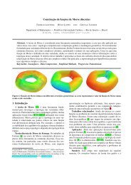
Particle-based non-Newtonian fluid animation for melting ... - PUC-Rio
Particle-based non-Newtonian fluid animation for melting ... - PUC-Rio
Particle-based non-Newtonian fluid animation for melting ... - PUC-Rio

Create successful ePaper yourself
Turn your PDF publications into a flip-book with our unique Google optimized e-Paper software.
A. Paiva, F. Petronetto, T. Lewiner and G. Tavares 2<br />
three topics.<br />
Smoothed <strong>Particle</strong> Hydrodynamics. The SPH method<br />
was introduced in the computer graphics community by Desbrun<br />
and Cani in [5], where they used SPH to simulate de<strong>for</strong>mable<br />
bodies. Müller et al. [19] then used the SPH approach<br />
<strong>for</strong> simulating incompressible <strong>fluid</strong>s with surface tension.<br />
Furthermore, they introduced point–splatting to capture<br />
the <strong>fluid</strong> free surface. Recently SPH methods became very<br />
popular in the special effects industry where it was used to<br />
simulate lava flow in the third part of The Lord of the Rings<br />
trilogy (http://www.nextlimit.com).<br />
Non–<strong>Newtonian</strong> <strong>fluid</strong>s. There are few works in computer<br />
graphics <strong>for</strong> <strong>non</strong>-<strong>Newtonian</strong> <strong>fluid</strong>s. Goktekin et al. [6]<br />
proposed a grid–<strong>based</strong> method to compute the stress tensor<br />
of these <strong>fluid</strong>s. They use a linear Maxwell model with<br />
von Mises plastic yield condition. Clavet et al. [3] use SPH<br />
with a linear combination of elastic springs between particles<br />
driven plastic yield condition. Another method using SPH<br />
was proposed by Mao and Yang [11], where the stress tensor<br />
derives from a corotational Maxwell model.<br />
Melting. The idea of simulating <strong>melting</strong> and flowing of<br />
solids objects by coupling viscosity with temperature appeared<br />
in different contexts. Carlson et al. [2] use an Eulerian<br />
grid-<strong>based</strong> <strong>fluid</strong> method. They further need an implicit<br />
integrator to compensate the instability of the grid–<strong>based</strong> approach.<br />
Wei et al. [22] use cellular automata and replace<br />
Navier–Stokes equations by simple rules in each automata.<br />
Müller et al. [20] create a point–<strong>based</strong> framework to simulate<br />
elastoplastic objects with von Mises plastic yield condition.<br />
They use moving least squares (MLS) <strong>for</strong> approximating the<br />
velocity gradient. Finally, Keiser et al. in [8] introduces traditional<br />
SPH method in the previous framework with usual<br />
viscoplastic modeling.<br />
Contributions. This paper introduces two new elements to<br />
the <strong>melting</strong> simulation. First, we use General <strong>Newtonian</strong><br />
Fluid model [12] to compute the viscosity (see Section 2).<br />
Its concise <strong>for</strong>mulation reduces the number of parameters <strong>for</strong><br />
yield modeling and allows simpler relation with the temperature.<br />
Moreover, since this <strong>for</strong>mulation covers viscoplastic<br />
<strong>fluid</strong>s within a single equation, it treats the whole object at<br />
once and avoids delicate detection of the viscosity transition.<br />
Moreover, we introduce in the heat equation approximation<br />
a more stable Laplacian operator on the particles (see<br />
Section 3). This approximation already improved Poisson<br />
simulations [4] by involving differences of first derivatives<br />
instead of second derivatives.<br />
We also introduce several numerical improvements in the<br />
method. First, we introduce the use of XSPH [14] <strong>for</strong> avoiding<br />
the <strong>for</strong>mation of stable clusters of particles (see Section<br />
3). Then, we reintroduce the artificial viscosity [5], but<br />
<strong>for</strong> <strong>melting</strong> simulation. We also chose the continuity equation<br />
<strong>for</strong> density (equation (6)) to avoids particle outliers.<br />
Finally, our implementation uses an adaptive time step <strong>for</strong><br />
each iteration <strong>based</strong> on the Courant-Friedrichs-Lewy condition<br />
(see Section 4).<br />
2 Formulation of the physical laws<br />
Computational <strong>fluid</strong> dynamics (CFD) aims at prediction<br />
<strong>fluid</strong> behavior through Navier–Stokes equations. These equations<br />
are commonly solved using conventional Eulerian <strong>for</strong>mulation<br />
with grid-<strong>based</strong> methods such as finite differences<br />
and finite elements. In this work, we chose an alternative<br />
method driven by the Lagrangian <strong>for</strong>mulation. As opposed<br />
to the Eulerian approach, the Lagrangian <strong>for</strong>mulation does<br />
not require advective term, which suits well <strong>for</strong> meshless<br />
methods such as SPH. We will introduce now this <strong>for</strong>mulation<br />
and the General <strong>Newtonian</strong> Fluid model [12] that models<br />
our viscoplastic object, together with our heating model.<br />
The reader will find further details on CFD in Anderson’s<br />
book [1].<br />
Lagrangian <strong>for</strong>mulation. Navier-Stokes equations can be<br />
<strong>for</strong>mulated by the following two equations describing the<br />
conservation of the mass (equation (1)) and of the momentum<br />
(equation (2)).<br />
dρ<br />
= −ρ∇.v (1)<br />
dt<br />
dv<br />
dt = − 1 ρ ∇p + 1 ∇.S + g (2)<br />
ρ<br />
where t denotes the time, v the velocity vector, ρ the density,<br />
p the pressure, g the gravity acceleration vector and S the<br />
viscoplastic stress tensor. This last term plays a fundamental<br />
role in <strong>melting</strong> simulation.<br />
Generalized <strong>Newtonian</strong> Fluid model. For <strong>non</strong>-<strong>Newtonian</strong><br />
<strong>fluid</strong>s, the stress tensor is a <strong>non</strong>linear function of the de<strong>for</strong>mation<br />
tensor D = ∇v + (∇v) T . For our simulation, we<br />
will use the Generalized <strong>Newtonian</strong> Liquid model proposed<br />
by Mendes et al. [12], where the stress tensor S is given by<br />
S = η (D) D, where the apparent<br />
√<br />
viscosity η depends on the<br />
1<br />
intensity of de<strong>for</strong>mation D =<br />
2 · trace (D)2 . The viscosity<br />
function η is then given by:<br />
(<br />
η (D) = (1 − exp [− (J + 1) D]) D n−1 + 1 )<br />
(3)<br />
D<br />
where n is the behavior of power–law index and J is the<br />
jump number.<br />
The jump number J is a new rheological parameter of a<br />
viscoplastic <strong>fluid</strong> which combines previous ones such as the<br />
yield stress and the consistency index. In our simulation, we<br />
fixed n = 1 2<br />
, and let only the jump number J vary with the<br />
temperature.<br />
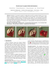
Heating and <strong>melting</strong>. The <strong>melting</strong> of volumetric objects<br />
corresponds to a phase transition from solid to <strong>fluid</strong>. We<br />
can model this transition by varying the viscosity according<br />
to the temperature of each particle. This model was used<br />
in other <strong>animation</strong> frameworks, either using grid-<strong>based</strong> approach<br />
[2] or particle-<strong>based</strong> approach [8].<br />
The time variation of the temperature is described by the<br />
The corresponding work was published in the proceedings of the Sibgrapi 2006, pp. 78–85. IEEE Press, 2006.