Transactions

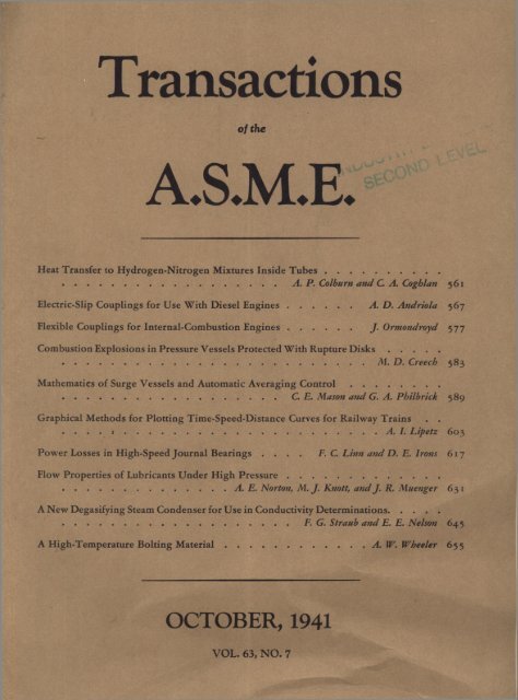
Transactionsof theHeat Transfer to Hydrogen-Nitrogen Mixtures Inside T u b e s ............................................................................................................................. A. P. Colburn and C. A. Coghlan 561Electric-Slip Couplings for Use With Diesel E n g in e s ........................ A. D. Andriola 567Flexible Couplings for Internal-Combustion Engines J. Ormondroyd 577Combustion Explosions in Pressure Vessels Protected With Rupture D i s k s ....................................................................................................................................... Al. D. Creech 583Mathematics of Surge Vessels and Automatic Averaging C o n t r o l ................................................................................................................... C. E. Mason and G. A. Pbilbrick 589Graphical Methods for Plotting Time-Speed-Distance Curves for Railway Trains . .A. I. Lipetz 603Power Losses in High-Speed Journal Bearings . . . . F. C. Linn and D. E. Irons 61 7Flow Properties of Lubricants Under High P re ssu re ........................................................................................................................ A. E. Norton, M. J. Knott, and J. R. Muenger 6 3 1A New Degasifying Steam Condenser for Use in Conductivity Determinations......................................................................................................... F. G. Straub and E. E. Nelson 64 5A High-Temperature Bolting M a t e r ia l..................................................... A. W. Wheeler 6 55OCTOBER, 1941

Transactionsof The American Society of Mechanical EngineersPublished on the tenth of every month, except March, June, September, and DecemberOFFICERS OF THE SOCIETY:W illia m A. H a n lb y , PresidentW . D. E n n is , TreasurerC . E . D a v ies, SecretaryCOMMITTEE ON PUBLICATIONS:C . B. P eck , ChairmanF. L. B r a d le y A. R. S te v e n s o n , J r .C . R . SODERBERGG e o rg e A. S te ts o n , EditorE . J . K aTESADVISORY MEMBERS OF THE COMMITTEE ON PUBLICATIONS:W . L . D u d le y , S e a t t l e , W ash . N . C. E b a u g h , G a in e s v ille , F l a . O . B. S c h ie r, 2 n d , N e w Y o rk , N . Y.Junior MembersC. C . K irb y , N e w Y o r k , N . Y . F r a n k l i n H . F o w le r , J r . , C a l d w e l l , N . J .Published m onthly by T h e A m erican Society o f M echanical Engineers. P ublication office at 20th and N ortham pton Streets, Easton, Pa T he editorialdepartm ent located at the headquarters o f the Society, 29 W est T hirty-N inth Street, N ew Y ork, N . Y. Cable address, "D ynam ic,” New Y ork. Price $1.50a copy, $ 12.00 a year; to m em bers and affiliates, $ 1.00 a copy, $7.50 a year. Changes o f address m ust be received at Society headquarters tw o w eeks beforethey are to be effective on the m ailing list. Please send o ld as w ell as new a d d ress.. . . By-Law: T h e Society shall not be responsible for statem ents o r opinion s advanced in papers o r ___ p rinted in its publications (B13, Par. 4 ) . . . . E ntered as second-class m atter M arch 2, 1928, at the Post Office at Easton, Pa.,u n d er the Act o f A ugust 24, 1912. . . . C opyrighted, 1941, by T h e A m erican Society o f M echanical Engineers.

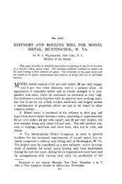
H eat T ran sfer to H ydrogen-N itrogenM ix tu res Inside T ubesB y A. P. COLBURN,1 NEWARK, DEL., a n d C. A. COGHLAN,2 BEACON, N. Y.This paper gives results of experim ents in w hich d atawere determ ined on h eat tran sfe r to air, to nitrogen, an dto eight m ixtures of hydrogen an d nitrogen, ranging from8.85 to 98 per cent hydrogen, flowing inside a steam -jacketed tube, 0.5 in. inside diam an d 48.75 in^. long. Therdata were well correlated when plotted asDG . Cpliv ersu s---- , w ith th e value of ——- ranging from 0.45 to 0.73.MKThe d ata checked h ea t-tran sfer d ata of N usselt an d showeddeviation from friction analogies.N o m e n c l a t u r eTHE following nomenclature is used in the paper:C, =c =D =/ =0 =h =j =k =% =Q a —

562 TRANSACTIONS OP THE A.S.M.E. OCTOBER, 1941F i q . 3 S c h e m a t ic A r r a n g e m e n to f E x p e r im e n t a l A p p a r a t u sF i g . 4 A ssem b l y o f E x p e r i­m e n t a l A p p a r a t u s a t G as-I n l e t E ndF iq . 5 A s s e m b ly o f E x p e r i.m e n t a l A p p a r a tc b a t G a s -O u t l e t E n d

COLBURN, COGHLAN—HEAT TRANSFER TO HYDROGEN-NITROGEN MIXTURES INSIDE TUBES 563F i g . 6 L o n g i t u d i n a l - S e c t i o nV i e w o f O u t l e t F r o m T e s t S e c ­t i o n , S h o w i n g S c h e m a t i c A s­s e m b l y o f T h e r m o c o u p l e U s e dt o M e a s u r e O u t l e t T e m p e r a ­t u r eboth gases and liquids, include the Prandtl number. For gasmixtures, however, one might question whether the proper valueto use is the Prandtl number of the mixture or some combinationof the Prandtl numbers of the pure components.If the Prandtl number of the gas mixture is the proper value touse in heat-transfer formulas, then data covering a range ofvalues of this number from 0.73 to 0.45 might make possible aselection of the best type of formula. Chilton (2) has shown aconvenient comparison of the exponential-type relation with thetheoretical relations of Prandtl (3) and of von Kdrmdn (4).These relations are different in the range of Prandtl numberscovered by these mixtures, and so the results should prove ofgreat interest in testing these equations.D e t a il s o f A p p a r a t u s U s e dThe apparatus chosen for this investigation was of the gas-intubestype, inasmuch as it was felt that the most reliable resultscould be obtained in such an apparatus. A stainless-steel tubewas used so that there would be no corrosion and change of surfaceconditions, and also because the low thermal conductivityof stainless steel would minimize heat conduction through theends of the appaj-atus. At the same time the thermal conductivityis sufficiently great to make the thermal resistance of the tubenegligible for the transfer of heat to the gas. The tube was steamjacketed,the outer cylinder being glass so that the type of condensationon the tube could be observed. The condensate fromthe tube was collected in a trough located inside the steam spaceand led outside the apparatus. The condensate on the glassjacket, resulting from radiation losses, was drained separatelyand discarded. This arrangement was made in the attem pt toobtain good heat balances. Atmospheric steam was supplied tothe jacket, and some steam was continuously vented at both endsof the jacket to insure that no air would collect. The steam-inletpipe to the jacket is 1 in. diam and is located below the trough.These conditions permit a very low steam velocity into the exchangerand at an elevation such that any moisture in the steamwould not be carried into the trough in which the condensatefrom the tube collects.TA B LE 1 D IM E N S IO N S OF T E S T SE C T IO NStainless-steel tubeInchesInside diam eter................................................................................ 0.50Outside diam eter............................................................................. 0.63Total length....................................................................................... 142.75H eated length ................................................................................... 48.75Length of calming section............................................................ 87.25Unheated length a t outlet end.................................................... 6.75Distance between pressure ta p s ................................................. 52.50The arrangement of the apparatus is shown in Fig. 3. A smallblower was used to recirculate the gas, and coolers were insertedbefore and after the blower to bring the gas to room temperatureat the entrance of the test apparatus. The rate of flow of the gaswas measured by an orifice meter constructed with throat taps,according to the specifications of the Fluid Meters Report.The metering tube was 2 in. diam, and orifices used were of 0.375,and 0.255 in. diam. These were calibrated on air, using a calibratedgas-meter prover, and the coefficient was found to be 0.61.Dimensions of the test section are given in Table 1.The glass steam jacket was supported by Iaminated-bakeliteflanges, shown in Figs. 4 and 5, at the ends of the heated section,drawn together by tie rods outside the glass jacket. Theseflanges were made tight to the stainless-steel tube by packingglands. Owing to the low thermal conductivity of these flanges,very little heat could be conducted to the tube beyond the insidesurfaces of the flanges.The heat, given up by the steam in heating the gas, was determinedby measuring the condensate collecting in the trough anddraining through the sight glass at constant level. This amountwas corrected for the small amount of liquid collecting on theflanges above the trough, and for the small heat loss from thesight glass; this correction was determined by blank runs when nogas was flowing, and was found to be 0.0258 lb per hr.T e m p e r a t u r e D e t e r m in a t io nThe temperatures were determined as follows: The inlet-gastemperature was measured by a calibrated thermometer at theentrance to the calming section. This temperature was adjustedby the coolers to be identical with the room temperature adjacentto the calming section, so that no increase or decrease in the temperatureof the gas would take place before it reached the heatedportion of the tube. The outlet temperature was measured witha special thermocouple, shown in Fig. 6, which was constructedto minimize radiation errors and to insure good mixing of the gasbefore the thermocouple. I t was made so that it could be slidout of the way when pressure drops were measured. The aluminumtube K acted as a radiation shield. The mixing device Lconsisted of two “doughnuts” and one disk of copper held inplace by being soldered to copper wires. This mixer was thenpainted with a thermosetting bakelite varnish and cured, in orderto minimize heat conduction from the tube. Laminated-bakelitespacers M kept the thermocouple centered. The steam temperaturewas also measured with a thermocouple in the jacket, andchecked against barometric pressure.Commercial hydrogen and nitrogen were used, and the compositionof the mixture was determined immediately following aseries of runs by means of a Bureau of Mines apparatus. Althougha special packing gland was built onto the blower, therewas a slight leak at that point, and a small amount of air wouldleak into the apparatus. This was determined by analyzing themixture for oxygen. This amount, less than 1 per cent, was calculatedas nitrogen. The gas pressure in the system was essentiallyatmospheric. Actually, enough gas to cause a slight pressurewas supplied to the system at the beginning of a run. Thispressure soon dropped until atmospheric pressure prevailed at thestuffing box of the blower.R e s u l t s o f E x p e r im e n t sThe principal results of this investigation are given in Table 2and in Figs. 7 to 12. The reliability of the data is measured bythe heat balances, the deviations from which are given by the

564 TRANSACTIONS OF THE A.S.M.E. OCTOBER, 1941F iq. 7E x p e r im e n t a l R e s u l t s I n c l u d in g I s o t h e r m a l - F r ic t io nD a t a and H e a t - T r a n s f e r D a t a o n A irF i g . 10E x p e r im e n t a l R e s u l t s o n H e a t T r a n s f e r t o H ydro-g e n - N it r o g e n M ix t u r e s C o n t a in in g 86.8, 94.4, a n d 98 P e r C e n tH y d r o g e n b y V o l u m eF i q . 8 E x p e r im e n t a l R e s u l t s o n H e a t T r a n s f e r t o P u r eN it r o g e n a n d t o H y d r o g e n - N it r o g e n M ix t u r e s C o n t a in in g8.68 a n d 28.6 P e r C e n t H y d r o g e n b y V o l u m e F i g . 11 S u m m a r y o f E x p e r im e n t a l R e s u l t s o n H e a t T r a n s f e rto N it r o g e n a n d H y d r o g e n -N it r o g e n M ix t u r e sF i g . 9 E x p e r im e n t a l R e s u l t s o n H e a t T r a n s f e r t o H y d r o g e n -N it b o g e n M i x t u r e s C o n t a in in g 37, 4 2 .9, a n d 55 P e r C e n tH y d r o g e n b y V o l u m ecolumn of data (q„ — qa) / 9

COLBURN, COGHLAN—HEAT TRANSFER TO HYDROGEN-NITROGEN MIXTURES INSIDE TUBES 565RunNo.GasT A B LE 2E X P E R IM E N T A L DATA^1 t 2 t .F F F6cl b p e rh rA 1 A ir * 7 4 .4 1 9 0 .4 2 1 1 .8 0 .2 1 32 7 5 .6 1 9 0 .4 2 1 1 .8 0 .2 4 73 7 5 .0 1 8 9 .0 2 1 1 .8 0 .3 1 14 7 5 .2 1 8 7 .0 2 1 1 .8 0 .3 7 35 7 5 .2 1 8 4 .8 2 1 1 .8 0 .4 4 36 7 5 .2 1 8 3 .8 2 1 1 .8 0 .5 3 6B 1 A ir** 7 5 .3 1 8 9 .4 2 1 1 .6 0 .1 9 02 7 6 .1 1 8 9 .8 2 1 1 .0 0 .1 7 53 7 4 .9 1 8 8 .0 2 1 1 .6 0 .2 6 14 7 5 .3 1 8 6 .7 2 1 1 .0 0 .2 9 15 7 4 .3 1 8 6 .2 2 1 1 .6 0 .3 5 26 7 3 .4 1 8 4 .0 2 1 1 .1 0 .3 8 97 7 4 .8 1 8 3 .7 2 1 1 .0 0 .4 3 38 7 5 .3 1 8 3 .3 2 1 1 .0 0 .4 2 99 7 4 .7 1 8 1 .3 2 1 1 .3 0 .5 2 610 7 3 .4 1 8 0 .4 2 1 1 .0 0 .5 3 311 7 5 .6 1 7 9 .3 2 1 1 .3 0 .5 9 5C 1 N3 6 7 .1 1 8 8 .8 2 1 2 .4 0 .2 4 52 6 7 .1 1 8 8 .0 2 1 2 .2 0 .2 5 53 6 8 .4 1 8 5 .8 2 1 2 .4 0 .3 1 84 6 7 .5 1 8 5 .0 2 1 2 .4 0 .3 7 65 6 7 .5 1 8 3 .3 2 1 2 .6 0 .4 6 16 6 9 .3 1 8 0 .0 2 1 2 .4 0 .5 6 37 7 3 .0 1 7 9 .2 2 1 2 .8 0 .6 5 4D 1 8 .8 5 $ 7 4 .5 1 9 3 .0 2 1 1 .1 0 .2 8 52H2 7 4 .5 1 9 0 .6 2 1 1 .1 0 .3 5 33 7 4 .5 1 8 8 .4 2 1 1 .1 0 -4 6 54 7 4 .3 1 8 6 .4 2 1 1 .1 0 .5 2 95 7 4 .1 1 8 5 .3 2 1 1 .1 0 .5 9 56 7 3 .8 1 8 3 .6 2 1 1 .1 0 .6 3 77 7 4 .3 1 8 3 .8 2 1 1 .3 0 . 713E 1 2 8 .6 # 7 4 .8 1 9 7 .8 2 1 2 .0 0 .3 2 22 «3 7 5 .0 1 9 5 .4 2 1 2 .0 0 .4 5 13 7 4 .1 193 .8 2 1 2 .0 0 .5 2 94 7 5 .3 1 9 2 .0 2 1 2 .0 0 .6 2 85 7 4 .8 1 9 0 .6 2 1 2 .0 0 .7 5 56 7 3 .3 1 8 9 .8 2 1 2 .0 0 .8 0 3F 1 37* 7 3 .0 1 9 5 .2 2 1 2 .0 0 .2 1 62 H3 7 1 .8 1 9 7 .2 2 1 2 .0 0 .4 3 03 7 3 .3 1 9 5 .6 2 1 2 .0 0 .5 5 24 7 3 .5 1 9 3 .8 2 1 2 .0 0 .6 3 85 7 3 .7 1 9 2 .4 2 1 2 .0 0 .7 3 56 7 0 .5 1 9 1 .6 2 1 2 .0 0 .8 4 4G 1 4 3 .9 $ 7 3 .4 1 9 8 .8 3 1 1 .1 0 .3 0 42 Hs 7 4 .3 1 9 8 .4 2 1 1 .3 0 -4 6 83 7 3 .6 1 9 6 .4 2 1 1 .3 0 .6 1 04 7 3 .7 1 9 5 .2 2 1 1 .3 0 .6 8 35 7 3 .7 1 9 4 .0 2 1 1 .3 0 .7 9 46 7 3 .6 1 9 3 .2 2 1 1 .5 0 .9 2 07 7 3 .4 1 9 1 .6 2 1 1 .3 1 .0 0 6H 1 55% 7 3 .8 1 9 1 .6 2 1 2 .0 0 .2 6 32 H3 7 3 .6 201 . 0 2 1 2 .0 0 .3 6 53 7 3 .8 2 0 0 .2 2 1 2 .0 0 .4 6 04 7 1 .1 199 *0 2 1 1 .3 0 .5 1 85 7 1 .6 1 9 7 .82 1 1 .3 0 .6 5 66 7 2 .0196 .6 2 1 1 .5 0 .7 2 27 7 2 .01 9 5 .22 1 1 .8 0 .8 3 3I 1 8 6 . 8j£ 7 3 .7 2 0 0 .62 H3 7 3 .9 192 .23 , 7 3 .1 2 0 0 .04 7 3 .2 1 9 9 .55 7 1 .4 197 .82 1 2 .0 0 .3 1 32 1 2 .0 0 .4 4 92 1 2 .0 0 .6 1 62 1 2 .0 0 .7 5 02 1 2 .0 0 .9 5 5J 1 9 4 .4 5 7 1 .4 1 9 8 .8 2 1 1 .5 0 .3 3 12 H3 7 3 .5 1 8 8 .4 2 1 1 .5 0 .4 5 53 7 2 .1 1 8 7 .02 1 1 .5 0 .5 5 84 7 1 .0193 .02 1 1 .5 0 .6 7 05 7 1 .4 1 9 4 .2 2 1 1 .5 0 .8 8 5K 1 98JS 7 1 .6 1 9 6 .2 2 1 1 .7 0 .3 7 52 h 3 7 1 .3 1 8 7 .22 1 1 .7 0 .4 5 53 7 3 .81 8 4 .62 1 1 .5 0 .5 7 94 7 3 .81 9 0 .62 1 1 .5 0 .7 2 45 7 3 .71 9 2 .02 1 1 .5 0 .8 2 96 7 3 .31 9 2 .02 1 1 .5 0 .9 1 8*Alr from compressed air line.**Air recirculated by 'blower.C A LC U LA TE D R E SU L T Swl b p e rh rq Gx 100jDG6 .4 8 0 . 0 0 .0 0 3 8 8 38007 .6 5 + 1 .0 0 .0 0 3 8 6 44909 .9 0 +1 .1 0 .0 0 3 7 3 58201 2 .3 3 +0 . 2 0 .0 0 3 5 5 73001 5 .2 2 - 1 . 3 0 .0 0 3 3 8 90501 7 .3 4 + 1 .8 0 .0 0 3 3 1 109505 .2 3 + 1 1 .3 0 .0 0 3 7 8 30506 .1 6 - 1 3 . 8 0 .0 0 3 8 6 36008 .2 9 + 5 .8 0 .0 0 3 6 5 48409 .6 5 - 0 . 4 0 .0 0 3 5 8 56401 1 .6 2 + 1 .2 0 .0 0 3 5 3 68001 3 .8 5 - 4 .8 0 .0 0 3 3 8 81001 5 .1 0 + 0 .9 0 .0 0 3 3 7 88001 6 .2 1 - 6 . 4 0 .0 0 3 3 3 95001 8 .4 0 + 2 .8 0 .0 0 3 1 5 107501 9 .1 0 0 . 0 0 .0 0 3 1 3 112002 1 .9 0 + 1 .3 0 .0 0 3 0 0 128006 .6 5 + 5 .0 0 .0 0 3 7 8 40507 .8 0 - 3 .9 0 .0 0 3 7 3 48009 .5 5 + 0 . 3 0 .0 0 3 6 0 58801 1 .6 5 - 0 . 7 0 .0 0 3 4 6 71601 4 .1 1 + 3 .0 0 .0 0 3 3 3 87001 8 .4 4 + 1 .6 0 .0 0 3 1 0 113402 2 .7 0 - 0 . 2 0 .0 0 3 9 8 149507 .8 1 - 1 .2 0 .0 0 3 7 3 51309 .9 1 - 2 .3 0 .0 0 3 5 9 65101 3 .1 7 + 4 .3 0 .0 0 3 3 9 86401 5 .8 0 + 0 .8 0 .0 0 3 3 4 103601 8 .2 1 - 0 . 2 0 .0 0 3 1 5 119502 0 .1 5 + 1 .8 0 .0 0 3 0 4 122402 2 .0 7 + 1 .9 0.00.297 144806 .9 2 + 3 .8 0 .0 0 3 7 8 46409 .9 3 + 1 .8 0 .0 0 3 5 2 66S01 2 .0 0 + 0 . 4 0 .0 0 3 3 9 80501 4 .4 0 + 2 .6 0 .0 0 3 2 1 96601 7 .5 8 + 2 .5 0 .0 0 3 1 1 117901 8 .8 8 + 1 .2 0 .0 0 3 0 5 126704 .2 3 - 7 .1 0 .0 0 3 4 3 2900a . 38 - 2 .4 0 .0 0 3 6 3 57601 0 .9 0 - 0 .4 0 .0 0 3 4 6 74901 2 .9 7 - 1 .1 0 .0 0 3 3 0 89001 5 .1 5 - 0 . 5 0 .0 0 3 1 7 104001 6 .9 0 + 1 .4 0 .0 0 3 1 3 116105 .0 5 + 2 .3 0 .0 0 3 8 0 35008.13* - 3 .3 0 .0 0 3 7 3 55401 0 .7 2 - 6 .6 0 .0 0 3 5 0 74301 2 .1 6 + 3 .5 0 .0 0 3 3 8 84301 4 .3 7 + 3 .2 0 .0 0 3 3 7 99701 6 .4 6 + 5 .6 0 .0 0 3 1 9 114201 7 .9 4 + 7 .7 0 .0 0 3 0 8 134503 .6 4 + 4 .7 0 .0 0 3 9 3 36305 .1 6 - 2 .1 0 .0 0 3 8 7 37306 .4 4 + 1 .4 0 .0 0 3 7 5 46407 .4 0 + 0 . 3 0 .0 0 3 7 3 53309 .0 4 + 5 .0 0 .0 0 3 5 8 65301 0 .3 8 + 2 .3 0 .0 0 3 4 1 74701 2 .1 5 + 2 .6 0 .0 0 3 3 6 87501 .7 9 - 4 .4 0 .0 0 3 7 3 16902 .7 2 - 1 .5 0 .0 0 2 9 0 25803 .7 9 - 7 .3 0 .0 0 3 6 5 36004 .6 7 - 7 .4 0 .0 0 3 5 8 44305 .8 8 - 0 . 4 0 .0 0 3 4 1 55801 .3 0 - 7 .0 0 .0 0 4 0 8 14451 .8 4 - 2 .4 0 .0 0 3 0 7 30302 .2 9 - 1 .4 0 .0 0 2 9 7 25252 .6 7 - 3 .7 0 .0 0 3 4 7 29402 .04 - 8 .6 0 .0 0 3 5 8 31301 .1 0 - 1 0 .3 0 .0 0 3 9 2 13171 .5 6 - 1 6 .4 0 .0 0 3 3 0 18681 .9 0 - 8 . 7 0 .0 0 3 0 9 22812 .2 1 - 5 .6 0 .0 0 3 5 6 26412 .4 7 - 4 .1 0 .0 0 3 7 0 29613 .7 0 - 6 .0 0 .0 0 3 7 1 3330Fdata of Nusselt (6, 7) The friction data areshown in Fig. 7 to be in excellent agreementwith the literature. In order to check a possibleeffect of the blower in recirculating thegases, heat-transfer data on air were obtainedby using both air from the compressed-airline in the laboratory (where fluctuationshad been well smoothed out by a surge tankand some 100 ft of pipe) and air recirculatedby the blower. There is no appreciabledifference in the results as will be seenfrom Fig. 7, and, furthermore, the data areseen to be in excellent agreement with thoseof Nusselt.A plot of data on pure nitogen, shown inFig. 8, is practically identical with that of thedata on air shown in the previous figure. Incalculating Reynolds’ numbers, values of viscositywere obtained from Fig. 1 and thencorrected to the mean gas temperature inthe tube, the latter correction meaning anincrease in the value of viscosity by about 10per cent.Data on mixtures of hydrogen and nitrogenare shown in Figs. 8 to 12. In calculating theordinates for these plots, values of the Prandtlnumber for the mixtures were taken fromFig. 2. For these gases, the value of Prandtl’snumber is practically independent of pressureand temperature over moderate ranges,so that the values given in Fig. 2 for 70 F couldbe satisfactorily used for the temperaturesencountered in these experiments. The closeagreement of the results in Figs. 8 to 12,with the previously plotted data on air, andwith the line representing the Nusselt airdata, is proof that the proper value touse in calculating heat transfer for mixturesis the value of the Prandtl number of themixture.As final indication of the necessity of includingthis factor, Fig. 12 shows h/ (CVG) plottedversus Reynolds’ number. The strong divergenceof the lines for the different mixturesproves the importance of the Prandtl numberof the mixture in bringing the results intoagreement.The effect of the Prandtl number can beshown, from the results in Fig. 12, to be atleast as important as the 2/a power, as oftenused in the exponential formula.......«In the range of values of Prandtl’s numberbetween 0.45 and 0.7, the Prandtl equationwould predict about one half this effect, andthe von K&rmdn equation something in betweenas shown by Chilton (2). While theseresults in themselves may not be sufficient todisprove these latter two equations, they areat least indications that the simple exponentialtype is more satisfactory for gas mixtures

566 TRANSACTIONS OF THE A.S.M.E. OCTOBER, 1941than the more theoretical ones, and suggest that further improvementsin the theory are possible.These data also verify the Nusselt data on gases in showing adeviation from the analogy between fluid friction and heat transfer.If this analogy (7) held, the heat-transfer and friction lines onthe plots would be coincident in the turbulent region. At lowReynolds’ numbers, the divergence may possibly be explained bythe presence of a greater “dip” region for heat transfer betweenviscous and turbulent flow than for friction. However, in thestrong turbulent region, the heat-transfer factors are still a good10 per cent below the friction factors. Above a Reynolds numberof 10,000 the slope of the line representing the heat-transfer data is—0.2 but at lower Reynolds’ numbers this slope becomes zeroand then of opposite direction in the “dip” region.There are a few results for the mixtures in the region of viscousflow, and while these seem to bear out the general shape ofcurves in the “dip” region and in the viscous region, there are notsufficient data to draw definite conclusions, other than that thePrandtl number appears as calculated.While the results of this study, together with those of Brunot(1), appear to, prove that the Prandtl number applies for gasesaccording to Equation [1], they show that further study of theanalogies between fluid friction and heat transfer is highly desirable.BIBLIOGRAPHY1 “Properties of Hydrogen M ixtures," by A. W. Brunot, Trans.A.S.M .E., October, 1940, pp. 613-616.2 “Engineering in the Service of Chem istry,” by Thomas H.Chilton, Industrial and Engineering Chemistry, vol. 32, January, 1940,pp. 23-31.3 “ Eine Beziehung zwischen W arm eaustausch und Stromupgswiderstandder Fliissigkeiten,” by L. Prandtl, Physikalische Zeitschrift,vol. 11, 1910, pp. 1072-1078.4 “ The Analogy Between Fluid Friction and H eat Transfer,” byT h. von Kdrmfin, Engineering, vol. 148, 1939, pp. 210-213.5 “ The Friction Factor for Clean Round Pipes,” by T . B. Drew,E. C. Koo, and W. H. McAdams, Trans. American Institute of ChemicalEngineers, vol. 28, 1932, pp. 56-72.6 “ Der W armeilbergang in Rohrleitungen,” by W. Nusselt,V.D .I. Mitteilungen uber Forschungsarbeiten, H eft 89, 1910, pp.1-38; also Zeit. V.D .I., vol. 53, 1909, pp. 1750-1755, 1808-1812.7 “A M ethod of Correlating Forced Convection H eat TransferD ata and a Comparison W ith Fluid Friction,” by A. P. Colburn,Trans. American Institute of Chemical Engineers, vol. 29, 1933, pp.174-209.D i s c u s s i o nR. H. N o r r i s . 4 It is of interest to compare the authors’ test resultsfor the region of viscous flow with theoretical results, eventhough, as the authors admit, their test data in this region are tooscanty to be conclusive.Fig. 13 of this discussion shows points representing the authors’test results compared with curves evaluated from a recentlypublished5 correlation of theoretical results, using the logarithmicmeantemperature difference basis. When the empirical correctionproposed by Colburn (7) for free convection is included, andthe possible range of error of the test results indicated by the heatbalancediscrepancy is allowed for, the agreement between testand theory is reasonably good (of the order of 10 per cent), belowReynolds’ number of 2200. For higher Reynolds’ numbers,transition to turbulent flow has presumably begun. The factthat the test values somewhat exceed the theoretical values mayindicate that the correction for free convection here applied to thelatter is not quite sufficient, or that the flow is not completelylaminar.4 General Engineering Laboratory, General Electric Company,Schenectady, N . Y. Jun. A.S.M.E.6 “Laminar-Flow Heat-Transfer Coefficients for D ucts,” by R. H.Norris and D. D. Streid, Trans. A.S.M.E., vol. 62, August, 1940, pp.525-533.

Electric-Slip Couplings for UseW ith Diesel EnginesBy A. D. ANDRIOLA,1 GROTON, CONN.T he fact th a t, in th e la st 12 m o n th s, a t least tw en tyD iesel-driven vessels have been equipped w ith electromagn etic-slip couplings in th is country in d icates its valuefor ship-propulsion purposes. T his paper explains th efu n ction s o f th e device as (1) to reduce torque-variationin ten sity a t th e reduction gears, and (2) to perm it tw o orm ore engines to be rapidly coupled and uncoupled to andfrom th e gearing to a com m on propeller sh aft. E lem entsof th e system are described and theoretical principles o fth e m echanism are analyzed. A b rief com parison is giveno f th e electric-slip coupling w ith th e hydraulic system .The paper concludes w ith m en tion o f addition al applications in con ju n ction w ith in tern al-com b u stion engines.THE progress made in Diesel-engine design, in terms ofreduced specific weight and size, has been achieved mainlyby substantial increases in rotative speed, working pressure,and number of cylinders per unit. This trend has brought tothe fore many important problems. Not the least of these isthat of dealing satisfactorily with torsional vibration.In marine installations, especially, two factors combine tomake this a problem of major importance: (1) The operatingrange extends over a large portion of the span from zero tomaximum speed. (2) Efficient propeller speeds are such as torequire a speed-reducing device when high-speed engines areused. Mechanical gearing is preferred because of the attendanteconomy, simplicity, and efficiency, as compared to other types.Experience, however, shows susceptibility to wear and failure,unless proper precautions are taken to limit vibration transmissionfrom the engine to the gearing. In special cases, thesedifficulties have been entirely obviated by the adoption of theDiesel-electric system of propulsion. This alternative involvesa substantially higher first cost and a lower over-all efficiencyand does not recommend itself to wide commercial usage. Inthis connection, therefore, the recent use of electric couplings ingeared-marine-Diesel installations is of considerable interest.F u n c t io n s o f E l e c t r ic C o u p l in gBriefly, the electric coupling is a device for transmitting torqueelectromagnetically across an air gap, there being no mechanicalconnection between the coupling halves. Units of widely differentcharacteristics have been developed for various uses, but thetype which is being applied to marine service utilizes inductionmotorprinciples and is termed the electric-slip coupling.The idea of transmitting torque through an air gap is not new.As early as 1921, a coupling of this type intended for marineuse was built and tested by Sperry,2 but apparently was neverput into service. The first commercial application recorded is1Engineer in charge of Engine Calculating Department, ElectricBoat Company. Jun. A.S.M.E.2 “Compounding the Combustion Engine,” by E. A. Sperry,Trans. A.S.M.E., vol. 43, 1921, pp. 677-716.Presented at the National Meeting of the Oil and Gas PowerDivision, Asbury Park, N. J., June 19-22, 1940, of T h e A m e r ic a nS o c ie ty o p M e c h a n i c a l E n g i n e e r s .N o t e : Statements and opinions advanced in papers are to beunderstood as individual expressions of their authors, and not thoseof the Society.that made by the Swedish firm, Allmanna Svenska ElektriskaAktiebolaget, or A.S.E.A., in a pilot-boat installation in 1935.Use of the coupling on a large-scale basis has since proceededsteadily. In this country alone, at least twenty vessels, totaling48 units, were equipped last year. Credit for the particularembodiment of the marine type of coupling is also shared by theWestinghouse and Elliott Companies, whose engineers wereworking along identical lines at the same time as A.S.E.A.The primary functions of the device are (1) to reduce torquevariationintensity at the gears, and (2) to permit two or moreengines to be rapidly coupled and uncoupled to and from thegearing to a common propeller shaft. Several typical arrange-*ments are shown in Fig. 1. Incidental to these uses, other importantadvantages are simultaneously obtained in the way ofpower flexibility and vessel maneuverability, closely approximatingthose of the Diesel-electric drive. These have beendiscussed in part by Metz and Ericson3 and are of sufficient importanceto warrant restatement here; these are as follows:1 Increased reliability of the plant is achieved by the use ofa multiple-engined arrangement.2 Any one unit may be shut down for repairs without stoppingthe vessel. *3 Economic cruising at partial speeds is possible by operatingonly a portion of the available units.4 The engines may be conveniently warmed up at the dockprior to vessel departure.5 Maneuvering in close waters or during docking can be facilitatedby operating some of the engines in the ahead directionand the remainder astern. The coupling between gearing andeither set of units can be rapidly made or broken by means of asimple switch. An appreciable saving in starting air is therebyalso effected.6 When reversing, as in an emergency, there is no need towait until the inertia of the entire system is dissipated. Instead,the engines may be uncoupled, reversed, and torque applied tothe propeller shaft while the latter is still turning in the aheaddirection. The coupling is therefore capable of braking effect.An earlier analysis3 of coupling-torque transmission undervibratory conditions indicates that the action was not completelyunderstood. Nevertheless, the operating experience accumulatedsince establishes the coupling as very well suited to therequirements of Diesel geared drives. It has also indicatedother applications in which the coupling characteristics may proveadvantageous either as a vibration controller or as a clutch, orboth.E l e m e n t s o f E l e c t r o m a g n e t ic C o u p l in gFig. 2 shows the main components of the coupling in elementaryform. The unit consists of two concentric rotors, aset of slip rings and brushes, an external source of direct-currentsupply, and a control panel. One rotor is a multipole-magnetring with individual poles energized from the slip rings mountedon the supporting shaft. The second rotor comprises a short-3 “Electromagnetic Slip Couplings for Use With Geared DieselEngines for Ship Propulsion,” by G. L. E. Metz and N Ericson,Trans. Institute of Marine Engineers, vol. 49, 1937-*938, pp.237-248.

568 TRANSACTIONS OF THE A.S.M.E. OCTOBER, 1941F ig. 1F i g . 2T y p i c a l I n s t a l l a t i o n s o f E l e c t b i c - S l i p C o u p lin g s t oG e a e e d M a e i n e - D i e s e l P r o p u l s i o n S y s te mC o m p o n e n t P a r t s o f T y p ic a l E l e c t r o m a g n e t ic-S l ipC o u p l in g scircuited winding of the squirrel-cage type. As illustrated inFig. 2, the pole ring is shown on the outer rotor, but the positionof the windings may be reversed without affecting the action ofthe coupling. Both arrangements have been used in practice.From a structural standpoint, the short-circuited winding isinherently the more rugged of the two and should preferably beused as the driving rotor. Of the two arrangements, the latterresults in a higher natural frequency of the engine system; thisis generally desirable from a vibration point of view. Irrespectiveof position, the pole ring and the short-circuited memberare termed the “primary” and “secondary” windings, respectively,to denote the magnetic path.Torque transmission across rotors occurs electromagnetically.If the primary is energized, relative rotation of the two memberscauses the secondary conductors to cut across a magnetic fieldof alternating polarity. The currents thereby induced set up aninterrotor torque, tending to rotate the driven portion in thedirection of the driving rotor. It is clear that the two memberscan never rotate at the same speed for, without relative rotation,or slip, torque cannot be induced. Under normal conditions,however, slip is an extremely small percentage of the drivingspeed. At full load, for example, its magnitude is about 1 percent and torque-transmission efficiency is consequently high. Aset of typical slip-torque-coupling characteristics for full andpartial excitation values is shown in Fig. 3. Interrotor torquevaries from a linear function of slip at very low slip speeds to amaximum at from 7 to 10 per cent slip. Beyond this point, thecoupling characteristic is definitely unstable and application oftorque, in excess of the maximum shown, results in stalling. Forproper operation, the coupling must be designed so that thestalling torque is substantially above that to be transmitted.With Diesel engines, the normal torque variation at ratedload may approach ± 100 per cent, depending upon the numberof cylinders. A.S.E.A. practice is to design for 170 per cent offull mean torque; this value is somewhat higher than the torquevariation which obtains in Diesel units of six or more cylinders.F i g . 3E l e c t r ic -S l ip C o u p l in g T o r q u e-S l ip C u r v e s f o r V a r io u s P e r c e n t a g e s o p E x c it a t io n

ANDRIOLA—ELECTRIC-SLIP COUPLINGS FOR USE WITH DIESEL ENGINES 569F iq . 4E l e c t b ic -S l ip C o u p l in g T o b q u e -S l ip C u b v e s f o b V a b io u s E n g in e S p e e d sUnder very rapid torque variation, electrical effects momentarilyincrease the stalling point to about 300 per cent of ratedcapacity, further reducing the chance of instability under averagedriving conditions. The stalling feature of the coupling, however,is desirable since the maximum shafting stress can thus be heldto a predetermined limit. This is especially true of systemssubject to seizure on the driven portion of the system. Inmarine installations, a suddenly fouled propeller would constitutesuch a seizure. The stress imposed on the engine members undersuch conditions might conceivably cause failure in a mechanicallyintegral system.The induced-coupling torque depends only upon the actual slipbetween rotors, i.e., it is independent of engine speed. Consequently,at starting or low-speed conditions, the total torquewhich can be developed at the engine is available for load pick-up.Torque-slip curves for partial speeds are shown in Fig. 4; theincrease in torque at 100 per cent slip with decrease in enginespeed is clearly indicated.C o n s t r u c t io n S im il a r t o S q u ik b e l - C a o e M o t o rThe similarity between the coupling and the short-circuitedsquirrel-cage induction motor, as regards the general construction,electromagnetic action, and slip-torque characteristics, isreadily apparent. In fact the two units may be said to be practicallyidentical except as to the means used to obtain a rotatingflux. In the three-phase alternating-current induction motor,for example, three-phase alternating current is supplied to thestator windings and produces a rotating flux with a speed dependentupon the supply frequency and the number of poles.In the electric-slip coupling, this is accomplished by mechanicalrotation of a direct-current excited-pole ring and the flux speedis equal to the mechanical speed of the primary rotor. Otherwise,the basic electrical considerations are the same for bothunits.Noticeable deviations from usual induction-motor practice areof a constructional nature and are dictated by mechanical considerationswhich the induction motor is not required to satisfy.These pertain to the method of rotor support, which has beenpreviously described as mechanically separated. Actually, thetwo rotors are overhung on their respective shafts, a pilot bearingbeing purposely omitted to accommodate a certain degree ofmisalignment between the driving and driven portions of thesystem. This construction requires use of an air gap appreciablylarger than for the induction motor. A.S.E.A. couplingsemploy air gaps of 0.2 to 0.4 in., depending upon the rated capacityof the coupling. Compared with induction-motor practiceof air gap = 0.15 \/K W the gap for a 1000-hp coupling isabout 4 times as large as that for a motor of identical capacity.The reluctance of the magnetic path is largely that of the air gap,and thus for equal flux densities the coupling requires a proportionatelylarger excitation energy. Nevertheless, excitationloss in the coupling does not exceed 1 to 2 per cent of the ratedcapacity. Over-all transmission efficiency, accounting for bothslip and excitation losses, is approximately 97 per cent. Theoverhung-rotor construction, however, does introduce a mechanicalproblem of some importance. When the two rotorsare displaced from the concentric position, the resultant eccentricityis accompanied by a proportional unbalanced radial pullin the direction of the smaller air gap. If unrestricted, this forcewould ultimately result in mechanical contact of the two rotorsaccompanied by magnetic locking. To avoid this effect, it isonly necessary to design the supporting shafts so that the loaddeflectioncharacteristic is steeper than the unbalanced pulleccentricityrelation of the rotors.Cooling requirements are met in a manner similar to th atemployed for motors. For this purpose a radial-bladed fan isbuilt into the outer rotor at its extreme edge as shown in Fig. 2.Openings in the end flange of this same member provide a naturalflow path for air over both windings. The effectiveness of thearrangement is a function of coupling speed. No difficulty,however, is encountered even when reasonably long sustainedperiods of operation at low speeds is a requirement, since the

570 TRANSACTIONS OF THE A.S.M.E. OCTOBER, 1941excitation current is normally reduced with correspondingly lessheat to be dissipated.M e t h o d o p C o u p l in g C o n t r o lCoupling control under operating conditions is quite simple.The coupling is made or broken instantaneously by operation ofa switch located at the engine control board. Thus, both engineand coupling are operated by the engine attendant. Normally,the excitation circuit is kept closed and the engines handledexactly as in a direct-connected installation. During dockingor channel maneuvering, the engines may be left running and thepropeller shaft controlled by means of the excitation switch.Where several units drive a common shaft, the load must bedivided equally among the engines, i.e., the slip at each couplingmust be the same. This latter quantity is measured by a simplestroboscopic arrangement and the necessary adjustment thenmade by variation of the fuel supply. The stroboscope consistsof two concentric bands with a number of equally spacedholes drilled in their peripheries. One band is carried on eachof the two coupling rotors. The relative rotational movementcan be clearly seen when a light source is placed within the innerband; measurement is then accurately made by a stop watch.Two years ago, the author had the opportunity to observe theoperation of two A.S.E.A. couplings during a trip of several days’duration aboard the Swedish motor vessel Astri. No occasionarose for an emergency-speed reversal, but all other normalmaneuvers at docking and in free route were carried out. Changesor reversals in speed were rapidly made without signs of shock orlag between engine and propeller speeds. Some of these operationswere timed and may be of interest; the interval measuredwas that from the initial telegraph bell to the moment thepropeller shaft reached speed, and includes the time taken bythe attendant to reset the telegraph prior to adjusting theengine throttle. Incidentally, the excitation circuit was keptclosed at all times. The values follow:FromStop‘/s Speed aheadStopToVj Speed aheadStopl/i Speed asternTime, sec101014These times represent average performance.When a wide operating speed range, of the order of 3 to 1, isused, the excitation current is usually reduced for low-speedoperation. This is done by means of an additional resistanceplaced in series with the excitation circuit. By such control,the efficiency of the coupling can be held approximately to aconstant value over the entire operating range.V ib r a t o r y C h a r a c t e r is t ic s o f C o u p l in gThe slip-torque characteristics previously discussed are thosewhich obtain under conditions of uniform driving torque. Actually,the torque delivered by the Diesel engine is periodic innature and may contain large variations from the mean value.The net motion at the driving rotor is a combination of harmonicmotions of differing frequencies superposed upon a uniformrotation. Tests, conducted on early installations, showed amarked suppression of oscillating motion across the coupling andthe action was interpreted as equivalent to that of a viscous-fluiddevice. Recent experimental and analytical data, however,show that the electrical effects which obtain under vibratoryconditions give rise to both elastic and damping components oftorque within the coupling. This effect was first brought to theauthor’s attention by G. J. Dashefsky of the New York NavyYard, who noticed the characteristic during tests conducted ona coupling furnished by the Westinghouse Company. Modeltests recently made available by the A.S.E.A. to the ElectricBoat Company and tests on a full-size coupling made at thelatter plant confirm Dashefsky’s observations. A mathematicalanalysis has also been developed by two members of the A.S.E.A.staff, Dr. Dreyfus and H. Arnemo, and is given in the Appendix.Values computed on this basis agreed closely with those obtainedexperimentally on the model coupling; these tests incidentallycovered a vibratory range from zero to 20 cycles per sec frequencyat the driving rotor. Since the preparation of this paper, asimilar mathematical analysis was presented to the AmericanInstitute of Electrical Engineers (A.I.E.E.) by Lory, Kilgore,and Baudry.4 This approach differs from that of A.S.E.A.,and, since a check of results is afforded, no duplication is involvedin presentation of the latter.F r e q u e n c y R a n g eThe frequency range of practical interest is considerably higherthan that covered in the model-coupling tests. Calculations foran 850-hp 460-rpm coupling have been made by the author upto a value of 100 cycles per sec. This corresponds to a naturalfrequency of 6000 vibrations per min and covers in general allcritical speeds of practical interest in marine drives. Thecomputed values are given in Fig. 5. At low frequencies, thedamping component is larger and the two become equal, in thisparticular design, at about 5 cycles per sec. Beyond this point,the decrease in elasticity is large compared to that of the damping.Both components may be considered as constant in valueabove 30 cycles per sec. In a previous reference,4 the elasticcharacteristic is compared to a weak mechanical spring, and thetendency is to treat the driving and driven systems as separateentities. While in many cases the treatment is perfectly applicable,it must nevertheless be noted that the term “weak” isa comparative one and therefore somewhat misleading. Inmarine installations, where a long length of shafting from theengine to the propeller is involved, it is possible for the line-shaftflexibility to exceed that of the coupling. While the conditionis not a usual one, its possibility shows that the device shouldonly be applied on the basis of a careful analysis of the entirevibratory system.Generally, the elasticity of both the driving and driven portionswill be quite low compared to that of the coupling. Theeffect of the coupling elasticity under these conditions is to introducean additional mode of vibration of very low frequency,compared to those of either portion treated separately. Thehigher modes of vibration correspond closely to those obtainedfor the separate portions of the system. In the fundamentalmode, all masses to one side of the coupling move practically inphase. The accompanying stress in the shafting is consequentlyvery low. Actually, the system is equivalent to one of twomasses, i.e., the driving and driven portions connected by thecoupling elasticity. The dynamic effect may be evaluatedsimply, if the damping between rotors is neglected. Let m =circular frequency of forced vibration; J\, Ji = driving anddriven inertias, respectively; K = coupling elasticity; p =circular frequency of natural vibration, i.e., p —\/[K (Ji + J^/JiJi]; M sin mt = vibratory torque deliveredto the driven member. Then it can be shown thatIn a twin-engined single-screw geared drive the phase relationbetween torque components delivered by each engine will modifyEquation [1] as follows: Introducing the additional notationr = vibratory order under consideration, = phase anglebetween similar cranks of the two engines, and Ji — moment of4 “ Electric Couplings,” by M. R. Lory, L. A. Kilgore, and R. A.Baudry, Trans. A.I.E.E., vol. 59, 1940, pp. 423-428.

ANDRIOLA—ELECTRIC-SLIP COUPLINGS FOR USE WITH DIESEL ENGINES 571F i g . 5 T o r s i o n a l a n d D a m p i n g C h a r a c t e r i s t i c s o f a n A . S . E .A . E l e c t r i c - S l i p C o u p l i n g ; 850 B h p , 460 R p minertia of each engine, we obtain (1) with both engines in phase,i.e., sin’ (i/-r/2) = 0(2) engines 180 deg out of phase, i.e., cos (

572 TRANSACTIONS OF THE A.S.M.E. OCTOBER, 1941At resonance m/p = 1, and Equations [5], [6], and [7] reduce toIf the predominant elasticity is that of the coupling, thisanalysis will yield rather accurate results. A comparison ofestimated and recorded values for a system with this dispositionof elasticity is given in Fig. 6. These data cover only the resonantrange controlled by coupling elasticity. At higher speedsno perceptible motion was recorded at the motor side of thecoupling. Sample torsiograms from 95 to 201 rpm are shown inFig, 7. Since these tests were performed with the motor drivingthe engine, the harmonic torque at the engine could be accuratelyestimated. The close agreement between analytical and testvalues thus directly confirms the electrical theory of the Appendix,by means of which the coupling characteristics were determined.For the higher modes of vibration the procedure is well knownand need not be discussed here.F i g . 6 C o m p a r i s o n o f E s t i m a t e d a n d R e c o r d e d V a l u e s f o rR e s o n a n t R a n g e s C o n t r o l l e d b y C o u p l i n g E l a s t i c i t yC o m p a r is o n o f E l e c t r o m a g n e t i c W i t h H y d r a u l i c C o u p l i n g sThe largest application of electric-slip couplings has thus far

ANDRIOLA—ELECTRIC-SLIP COUPLINGS FOR USE WITH DIESEL ENGINES 573been in geared marine drives of the multiple-engine single-screwtype, where rapid engine disengagement is desirable. The hydrauliccoupling has been similarly employed and a comparisonis of interest. Each coupling requires auxiliary equipment and,in this respect, both have disadvantages. In efficiency eachaverages about 97 per cent. For hydraulic couplings, the lossis approximately, a fixed percentage of speed, but the same istrue of the electric-slip coupling with economy-resistance control.For speeds below 400 rpm, the electric-slip coupling is definitelysuperior in weight and size. As more experience with the latteris obtained this limit may be raised considerably. The torquecapacity of the electric coupling varies as the diameter squaredtimes length of rotor, or D2L, and is independent of speed; inthe hydraulic coupling the variation is directly as (diameter)2 Xspeed. Within limits, the dimensions of the former may bevaried, provided D2L remains constant. The same facility islacking in the latter. The mechanically separated rotors of theelectric coupling eliminate the possibility of wear, therebyreducing maintenance. Hydraulic couplings of modem design,however, are relatively wear-free and no distinct advantage maybe claimed in this respect. As regards rapidity of couplingaction, however, the electric coupling has no equal. Wheredirect current is available, however, adoption of the electric-slipcoupling in preference to the hydraulic unit is indicated..Otherwise, with weight and size equal, choice appears to rest oncost.A d d it io n a l A p p l ic a t io n s o f E l e c t r ic -S l i p C o u p l in g sExclusive of geared applications, the coupling characteristicssuggest its use for several other services in which the intemalcombustionengine is employed. I t should be appreciated,a priori, that for a given torque-weight ratio, units with widelydifferent torque-slip properties can be constructed. The quantitativevalues, in Figs. 3 and 4, apply strictly to the shortcircuitedsquirrel-cage type. With a wound secondary connectedthrough slip rings to a variable resistance, for example,variable-slip-speed characteristics can be obtained. In general,for every known type of motor or generator, a correspondingelectric coupling is possible. Additional applications then fallinto the following categories:(а) Systems in which seizure of the driven members is likelyto occur, such as suction-dredge installation or vessels operatingin shallow or ice-filled waters.(б) Direct-drive marine installations required to operate atpropeller speeds considerably below one third maximum enginespeed. With a wound-rotor construction, slip speeds of the orderof 50 per cent are possible for short periods. The losses areapproximately proportional to slip but nevertheless small dueto the low powers developed in this speed range.(c) Drives requiring smooth-turning characteristics at theload. If in addition rapid clutch action is desired, maximumutility of the device is attained.From a vibration standpoint alone the electric-slip coupling,properly used, will effect a highly satisfactory drive. Comparableresults, however, are also possible with less expensivemechanical devices. Thus, unless some additional functionis to be performed, the greater cost involved is not usuallyjustified.A c k n o w l e d g m e n tAppendixThe following nomenclature is used in the Appendix:N o m e n c l a t u r ea — a0 sin mt = relative angular displacement betweencoupling rotors, radians = flux, maxwellsB = direct-current field, gaussL = length of iron, cmR = radius of air gap, cmS ,S ',S 'i = current densities, amp per sq cmp - resistance, ohmsf = frequency of oscillation of coupling rotors, cyclesper sec/* = a-c permeability of iron, gauss per oerstedT, = slot pitch, cmh, = tooth height, cma, = effective tooth area, sq cmn = tooth resistance, ohms= tooth reactance, ohmsi. t = conductor current, ampit = tooth current, amp2 = impedance, ohmsr. = conductor resistance, ohmsx. = conductor-leakage reactance, ohmsr = specific impedance, ohm per cm periphery per cmlengthh = sum of currents under pole arc, amps = magnetic air gap, cm6 = effective pole arc, cmh = inductance, hra = short-circuit ring resistance under pole arc, ohmsru = short-circuit ring resistance in space between poles,ohmse = induced voltage in secondary conductor, vSa = current density per unit periphery, amp per sq cmper cmh = length of short-circuit ring under pole arc, cmB = pulsating air-gap field, B includes B, gaussn = number of polesT = induced-coupling torque, kg-m3 = V = iThe author wishes to express his appreciation to Mr. E. Nibbs,chief engineer, Electric Boat Company, for permission to publishthe analysis given in the following Appendix. Also to E. S.Dennison and G. F. Dashefsky for helpful criticism and suggestions.The torque delivered by the engine to the driving rotor of thecoupling is a periodic function. Analytically it may, therefore,be considered as composed of a constant torque and a number ofharmonic-torque components of differing frequency. Transmissionof torque through the coupling then produces a constantslip between the rotors upon which is superposed a relativevibratory motion. In the following analysis the relative speeddifference, i.e., slip, is neglected. The relative angular displacementbetween rotors can then be written asa = ao sin m t.....................................[11]Provided no counteracting ampere turns are induced in eitherrotor, there arises in the secondary part of the coupling, in eachof the gaps between poles, a cross field, shown in Fig. 8 with aflux of2 = 2 B L R a ......................[12]Actually, the motion gives rise to eddy currents in the iron ofboth rotors, as well as currents in the cage winding, and theresultant pulsating field has a distribution as shown in Fig. 9.The a-c permeability n of the iron is a function of /L, Ra, and

574 TRANSACTIONS OF THE A.S.M.E. OCTOBER, 1941th e effective to o th area is th u sWithin the active length, tooth and conductor are connectedin parallel. Outside this length the conductor has an impedanceof Ar, — j Ax, and the effective impedance of one slot pitch isthusD i f f e r e n t i a l E q u a t io n s a n d T h e i r S o l u t io nThe sum of the currents I h under the pole arc produces a fluxof 2i in the interpolar space, i.e.F ig . 9D is t r ib u t io n o f P u l s a t in g F ie l dm, and is estimated according to previous investigations whichshow that for / cycles per sec and 50 cycles per secwhere the factor y and the inductance lk are determined by fieldplotting, as shown in Fig. 10.The a-c permeability in general will be rather high, especiallysince, at higher frequencies (see Fig. 9) is divided into „ alongthe pole-shoe surface and *along the short-circuit winding. Inview of this, the ampere turns consumed for the iron will beneglected.The fact that the teeth lead currents parallel to the cagewinding must, however, be taken into account since this willlessen its effective resistance and also influence its leakagereactance. The cage winding is not insulated. To a currentdensity S in the conductor there corresponds a current density

ANDRIOLA—ELECTRIC-SLIP COUPLINGS FOR USE W ITH DIESEL ENGINES 575D i s c u s s i o nM. R. L o r y . 5 Mr. Andriola is to be congratulated on hisinteresting and informative paper. The application of electriccouplings on a large scale has come so recently in this countrythat little has been written about them. This paper is a valuableaddition to the literature.It is fortunate that the author has included some informationfrom his associates at A.S.E.A. That company’s actual experiencein building couplings antedates our own by several yearsbecause geared-Diesel drive has been popular in Europe for sometime, while its use on a large scale is quite recent here. However,‘ Westinghouse Electric & M anufacturing Company, East P ittsburgh,Pa.we are now making rapid strides, as indicated by the fact thatthe writer’s company alone now has more total horsepower incouplings built or under construction than have been built orare on order abroad, based on the latest published information.*We are now building the largest electric couplings in the world,rated 4375 hp at 180 rpm, for use with Sun-Doxford engines onfour Maritime Commission CP-3 cargo and passenger vessels.Of the 62 motorships already built or on order on June 1, 1941,for the Maritime Commission, 38 have geared drives of which 30are equipped with electric couplings and 8 with hydraulic couplings,while 24 are direct drive.The principal difference between the electric couplings for theseMaritime Commission ships and foreign-built couplings is in theamount of torque available at high slip for maneuvering. Figs.3 and 4 of the paper show a coupling with 40 per cent torque at100 per cent slip. The Maritime Commission engineers recognizedthat, if more torque than this were provided, the couplingscould be used extensively as an aid in maneuvering. Consequently,their specifications required a minimum of 75 per centtorque up to 140 per cent slip.The Mormacpenn, first of four C-3 cargo ships built by theSun Shipbuilding and Drydock Company, and the first geared-Diesel ship to be completed under the Commission program, haselectric couplings. Each of these ships has four Busch-Sulzerengines rated 2230 hp at 240 rpm, driving through Westinghouseelectric couplings and Falk gears. The couplings on these shipshave proved very satisfactory in service. The ships are exceptionallyeasy to maneuver. The engine and coupling controlsare centralized in a control desk. The right-hand lever on thedesk controls the operation of all four couplings. The usual procedureis to warm up two engines ahead and two astern at the“stand-by” signal. Then the operator can carry out any maneuverexcept “full ahead” or “full astern” by means of thecoupling control and engine-speed levers. No starting air isconsumed and the ease of operation is comparable to Dieselelectricdrives. The writer has observed response to six bells in1 min when docking.The couplings on these vessels have about 100 per cent torqueat high values of slip. This enables a crash-stop reversal to bemade by disconnecting the engines from the propeller and reversingthem at no load. The couplings are then energized andreverse the propeller while the engines run on fuel. This methodof reversal is very fast and uses little starting air. The Mormacpennwas forced to make a crash stop in New York harbor toavoid a collision in a fog. The propeller was turning at higherthan full speed astern in less than 1 min. While this time wasshortened by the fact that the ship was not up to full speed aheadwhen the reversal was started, the quick reversal was creditedwith avoiding a crash. It is doubtful if a coupling with torque,as shown in the curves of the paper, would be able to reverse thepropeller from full speed.The writer was greatly interested in the mathematical analysisof the characteristics of the coupling which affect torsional vibration.When his company first studied electric couplings, someengineers recognized the torsional characteristics and worked upcurves similar to the author’s Fig. 5 for the Navy. Discussionsof torsional characteristics led up to the extensive tests made byMr. Dashefsky which were mentioned in the paper. It is impossibleto compare the formulas in the paper exactly with thosepublished4 by the writer and others because differences in constructionmodify the analysis. The A.S.E.A. couplings are builtof solid iron in the secondary core and the analysis must takecare of eddy currents induced in the iron parts. We use laminatedironcores and these eddy currents have negligible effect and were8 ^.iS.B.A. Journal, March, 1940.

576 TRANSACTIONS OF THE A.S.M.E. OCTOBER, 1941neglected in the analysis. The curves obtained show that thetwo methods give similar results.I t is hoped that the amount of mathematical work done indetermining the characteristics of electric couplings has notcreated the impression that torsional vibration presents a seriousproblem when they are used. Rather, the studies have beenundertaken so that the designer may calculate the characteristicsaccurately, and predict the performance. When we know how acoupling acts, we can apply it properly. The large number introuble-free active service constitutes the best proof that suchcouplings do protect the gears from torsional vibrations as wellas aiding in maneuvering and performing all their other functionsas discussed in the paper.The question has come up regarding the heating of the couplingsduring maneuvering; for example the chief engineer on oneScandinavian vessel has said that he could not maneuver withthe couplings because they overheated. It is not surprising thatthis happened with couplings which were not designed for thisservice.As mentioned previously, the Maritime Commission engineersare largely responsible for the use of the couplings for maneuvering.For their ships, they specified sufficient torque to enable thecouplings to perform this service, and also made sure th at thecouplings were adequate from a heating standpoint.During the maneuvering, the couplings act as clutches. Thereis no mechanical contact between the two members, and hencethere is no wear to cause maintenance. However, as in anyclutch when the slip is high, energy must be dissipated. Thisenergy appears as heat in the bars of the squirrel-cage winding.The time of operation at high slip is short, but the rate of heatgeneration is high, and little of the heat can flow out of the bars.A large portion of it has to be stored in the bars, and the onlyway to keep the temperature down is to provide a large mass ofmaterial to store the heat. For this reason, the bars must bemade as large as possible.This squirrel-cage winding is very rugged, since it consists ofbars driven into slots in the core, and brazed with a high-temperaturealloy at the ends to short-circuiting rings. There is noinsulation to roast out, and the winding can stand high temperartures without injury. The most severe operating condition isduring a reversal from full ahead when the couplings are disengagedwhile the engines are reversed and brought to about halfspeed astern. When the couplings are energized, they mustbring the propeller to rest and then pull it up to the engine speedastern. They are designed to do this with moderate temperaturerise, since margin must be provided to take care of any unusualoperating conditions which might increase the heating.During the trials of the eight Maritime Commission shipsusing electric couplings which have been completed, the couplingswere often subjected to service several times worse than anormal reversal without injury. On the trials and the severaltrips in active service, the couplings have been subjected toevery normal type of maneuver plus many abnormal ones withoutany damage of any kind from overheating.A u t h o r ' s C l o s u r eMr. Lory’s discussion constitutes an important addition to thematerial presented, especially as regards operating experiencewith couplings of this type.Since presentation of the paper, we have had the opportunityto study closely the operation of two couplings in a twin-screw,direct-drive installation. Maintenance has been conspicuous byits absence, although these units have been in service 8 monthsin addition to a continuous 17-day shop test at 80 per cent powerand 24 hours at full rating. While these couplings are not specificallydesigned to reverse the propeller from full speed, earlyship-board tests soon established their adequacy for this maneuver;the units have been so operated since. It should be recognized,however, that in the interval between coupling disengagementand re-engagement, a reduction in propeller-shaft speedand necessary reversing torque will have taken place. Theamount of reduction is a function of ship inertia and resistance.Mr. Lory properly emphasizes the true importance of the vibrationstudies made for these couplings, and the author earnestlyhopes that misinterpretation has not occurred as a result of thespace devoted to this aspect of design.

Flexible Couplings for Internal-C om bustionEnginesBy J. ORMONDROYD,1 ANN ARBOR, MICH.Four typical dynam ical cases of torsionally flexible“linear” couplings are exam ined: (1) In stan tan e o u sapplications of th e m axim um engine to rq u e; (2) in s ta n ­taneous stoppage of th e engine or th e driven m em ber;(3) dangerous torsional resonance; and (4) to o th c h a tte rin geared drives.THE basic purposes of any coupling are to tie together componentparts of a rotating assembly and to transmit theoperating torque safely between the parts. The wide diversityof coupling designs indicates that they are often expectedto be more than mere concatenating links and transmitters oftorque. Even when the component parts of the rotating assemblageare supposed to maintain fixed relative positions, theproblem of alignment has forced the design of couplings withvarious degrees of freedom compatible with carrying out theirbasic functions. A large class of couplings embodying elasticallyflexible elements exists. These couplings are not only expectedto concatenate component parts, transmit torque, and provide acertain amount of leeway in alignment, but they are also expectedto provide a protection to the rotating system which would notexist if the flexibility were omitted.The protection needed by the system is not always clear tothe design engineer. In general, flexible couplings are useful in“dynamic” situations in which angular velocities are changingor in which the driving or delivered torques are variable. Asecond generalization, which cannot be emphasized too strongly,is that a flexible coupling is embodied in a complete rotatingBystem, and its effects depend as much on the system characteristicsas on its own properties. Such data as hub size, installationdimensions, and allowable horsepower per hundred revolutionsper minute based on nominal load torque are necessary,but they are not sufficient to determine a successful application.The effect of a flexible coupling is measured by the differencein operation with the added flexibility and the operation withoutit. The difference to be expected can often be predicted bydynamic analysis of the whole rotating system with and withoutthe coupling.Four typical dynamical situations in which torsionally flexiblecouplings are often considered will be examined. In all casesthe coupling will be considered as “linear,” that is, the angulardeflection or twist between the driving and driven sides of thecoupling will be proportional to the torque transmitted in astatic test. The four cases are:1 Instantaneous application of the maximum engine torque.2 Instantaneous stoppage of the engine or the driven member.3 Dangerous torsional resonance.4 Tooth chatter in geared drives.torque. It is worse than any actual case can be. If a couplingcan be made to meet this situation safely, it will be more thanadequate to meet any rapidly rising torque. To simplify theproblem consider the engine as a single body of moment of inertia hand the driven member as another body of moment of inertiah. The coupling and other connecting shafting has an over-allspring constant K. The suddenly applied engine torque is T.Friction torque and load torque can be ignored since the maximumdistress in the connecting shafting will occur soon after theengine torque is applied and long before any load or friction torquecan be developed. Let $i be the motion of h and be the angleof twist in the coupling members. Under these assumptions,Newton’s second and third laws give the following equations ofThe maximum absolute value of the torque in the couplingmembers occurs when cos pt = —1. It isI n s t a n t a n e o u s l y A p p l i e d T o r q u eThis situation is an idealized limiting case of suddenly applied1 Professor of Engineering Mechanics, University of Michigan.Mem. A.S.M.E.Contributed by the Oil and Gas Power Division and presented a tthe Annual Meeting, New York, N. Y., Dec. 2-6, 1940, of T h eA m e r i c a n S o c i e t y o f M e c h a n i c a l E n g i n e e r s .N o t e : Statem ents and opinions advanced in papers are to beunderstood as individual expressions of their authors, and not thoseof the Society.The torque twisting the connecting members is independentof the spring constant of these members, depends on the ratioI J h , and can never be greater than 2T.Evidently, this is one dynamic problem in which a springcoupling offers no advantages. If the ordinary shafting whichconnects the two rotating members is made strong enough tostand twice the maximum possible torque that the engine canput out, everything has been done that can be done for thisparticular case.577

578 TRANSACTIONS OF THE A.S.M.E. OCTOBER, 1941I n s t a n t a n e o u s S t o p p a g e o f O n e R o t a t in g M e m b e rUsing the same system as before, there are two cases, dependingon which rotating member is stopped. In either case the entirekinetic energy of the free body must be stored in the elasticcoupling members, if the energy lost in frictional dissipation isignored. In these casesIn both equations w is the angular velocity of the entire rotatingsystem just before the sudden stoppage. In either casewhere n is either 1 or 2.The maximum twisting torque in the coupling member isIf Mo is the maximum torque with the usual rigid coupling andMt is the maximum torque with the flexible coupling in place,and K 0 is the original spring constant of the coupling shaftingand Kt is the spring constant of the flexible coupling, thenAny reduction in twisting torque desired can be made bychoosing Ki small enough. Naturally the coupling parts mustbe strong enough to withstand successfully the twisting torque M.This case is a particular instance of impact. If two absolutelyrigid bodies collide, the impact force is infinite in magnitude.If a spring is interposed between the bodies, the forces betweenthem become finite and controllable.T o r s io n a l R e s o n a n c eThis phenomenon has been treated extensively in technicalliterature and will not be discussed in detail here. The naturalfrequencies and “normal elastic curves” which can be calculatedby using the Holzer method familiar to many engineers arefruitful guides in judging the usefulness of flexible couplings inparticular cases. These data, usually determined for the caseof no frictional damping, must often be supplemented by estimatesof the effects of damping on the amplitudes and stresseswhich occur at resonance.In applying a flexible coupling to a rotating system its effectson more than the lowest natural mode of vibration of the systemmust often be considered. If the operating speed of the enginedrivensystem is constant, a flexible coupling will often sufficeto make operation at that speed free from dangerous amplitudesof motion. If the operating speed is variable, flexible couplingswithout damping devices are often “snares and delusions.”There are some systems in which a properly designed flexiblecoupling will put the lowest natural frequency of the systembelow the idling speed, and the next higher mode of motion mayhave its resonance above the running range; but many actualsystems, such as modern line airplane engines, are not so easilyhandled. The coupling may make one mode safe; but have noprotective value at all in another mode of motion.This problem presents an example of the influence of the entirerotating system on the operating characteristics of the flexiblecoupling.G e a r - T o o t h C h a t t e rConsider an internal-combustion engine driving a centrifugalpump through a step-up gear. An eight-cylinder line enginewith a maximum speed of 900 rpm will be considered. Since weare interested in general ideas, the system can be representedin the simplified form of three flywheels connected by two torsionalsprings. This system permits a general survey of thepossibilities of gear-tooth chatter at resonance in the one-nodcdmode of motion. It would not serve well to investigate thepossibilities in the two-noded mode of motion.Let Ii = the moment of inertia of the engine rotating partsh = the moment of inertia of the flywheelIs = the combined moment of inertia of the gearing andcentrifugal pump (all reduced to the engine-shaftspeed)Ki = the spring constant of the engine shaftK 2 = the spring constant of the connecting elementsbetween the flywheel and the slow-speed gear.This will include any flexible coupling which maybe used.The calculations made assume that the gear teeth remain incontact on one side even during resonance vibrations. In factthis is a necessary state of affairs if the gear is to operate quietly.It can be realized in practice if the maximum inertia torque ofthe pump and pinion never exceed the load torque transmittedthrough the gearing to the pump.It is proposed to make a preliminary survey of the vibrationand gear-chatter possibilities of this system by merely calculatingthe frequency and “normal elastic curve” without damping, usingthe usual Holzer method. The analysis proposed does not givethe actual amplitudes of motion which will be encountered inoperation at resonance. It merely gives an idea of the bestresults which can be attained by varying the parts of the system.The best that can be done by varying the flexibilities and momentsof inertia may not be good enough, in which case special devicesfor ameliorating the vibration conditions may have to be introducedinto the system. However, the operating conditions inmany systems have been made safe by simply varying the flexibleand inertia elements.Two major assumptions are made in the following calculations.They are:1 The damping in the system is unknown; but it is assumedto remain at or near the same value no matter what changesare made in the system.2 For the major critical speeds in the lowest mode of motionthe energy input per cycle is assumed to be proportional to theaverage of the relative amplitudes of motion of the engine hand the flywheel / 2.Based on these two assumptions the actual amplitudes encounteredwill be proportional to the average of the relative amplitudesof the engine and flywheel in any given combination considered.For the simplified system considered the single-noded frequency/ = p/2x can be calculated from

ORMONDROYD—FLEXIBLE COUPLINGS FOR INTERNAL-COMBUSTION ENGINES 579To make the problem concrete assume that the system isoriginally laid out so that 7i = 60 lb in. sec2; h = 200 lb in.sec2; I3 = 160 lb in. sec2, K\ = 5 X 106lbin. per radian; and K i =30 X 106 lb in. per radian. Substituting these values in theequations it is found that the one-noded, fourth-order criticalspeed will occur near 725 rpm and that the node (or point ofmaximum shear stress) lies in the crankshaft near the flywheel.Since the engine might operate at this speed this information isquite disturbing.By introducing a flexible coupling between the flywheel andthe gear, it may be possible to place the critical speed at a lowrunning speed and also the point of maximum twist may beshifted from the crankshaft into the coupling where damagewill be less expensive and more easily repaired. The effect ofvarying K\ by introducing additional flexibility is seen in Fig. 1.The data from Equations [13] to [16] also permit an estimateof the possibility for tooth chatter. If the actual moment ofinertia of the centrifugal pump and its pinion is 13', its equivalentvalue reduced to gear speed is n2l 3 , where n is the gear speed-upratio. The maximum inertia torque of the pump and pinion,referred to the gear, is n2I3'p2A 3. Since the actual value of A ,is proportional toi- i i n2I3'p2A 3(Ai + A 2)i s proportional t o -------------------------.‘ ^ — -, the actual value of the inertia torqueThe load torque transmittedthrough the gear is the pump-load torque. For a centrifugalpump this torque is T = CW2, where N is the engine rpmF ig . 2E f f e c t s o f V a r y i n g h , K i = 3 X 106 L b I n . p e r R a d i a nand C is a constant depending on the dimensions of the pump.order harmonic torque N 2 = — p2, then16F ig . 1 E f f e c t s o f V a r y in g K i, 1 2 = 200 L b In . S e c 2By reducing K i to one tenth of its original value it is possibleto depress the critical speed down to 400 rpm and to displace the Because n2, I 3’, and C are independent of changes in K i, it canlargest twist from the crankshaft into the coupling. The actual be seen that the tendency for the gears to chatter is proportionaltwist in the crankshaft is also reduced to about one half of its bOA 3{A\ + Ai).original value.From Fig. 1 it can be deduced that this quantity A 3(A i + Ai)This last conclusion follows from the fact that the actual amplitudeshas increased 10 to 1 as K 2 is reduced from 30 X 106 lb in. perand twists are proportional toThe relativeradian to 3 X 106 lb in. per radian. While this rough analysisdoes not indicate whether the gear teeth will actually chatter,twist in the crankshaft is Ai — A 2. The actual twist will then it does emphasize the fact that tooth chatter is far more likely tobe proportional to (Ai — A 2), or to A i2 — A 2 occur with the flexible coupling than without it. While the introductionof the coupling has reduced the stress in the crankshaftFor2 ‘ 2and lowered the critical speed to a range in which the engine istwo different values K i and K i' the relationship between actualless likely to run, it has increased the probability of gear noisetwists will beat this lowered critical speed enormously. Evidently, the intro­For K i = 30 X 106 lb in. per radian and AY = 3 X 10® lb in.per radian, this ratio is approximately one half.duction of additional flexibility without some other change inthe system may, in this case, merely change the problems encounteredin the design.What other characteristic of the system can be changed sothat the favorable changes introduced by the coupling can bemaintained while the unfavorable developments can be minimized?Naturally, the engine, gears, and pump are not easily

580 TRANSACTIONS OF THE A.S.M.E. OCTOBER, 1941modified. The flywheel is a member which can be modifiedwithout undue practical difficulty. Fig. 2 indicates the changeof conditions brought about by varying 7j from 200 lb in. sec2 to20 lb in. sec2, keeping K i constant at 3 X 10* lb in. radian. ForIi = 20 lb in. see2 the value of N is not raised much nor is theactual twist in the engine shaft changed much; but the valueof (Aj + AijAs is reduced to one third of its value for = 200lb in. sec2. While this value is still three times greater than itwas in the original design, it is a large change in the right direction.A further change which could be investigated would be theintroduction of an additional flywheel between the flexiblecoupling and the slow-speed gear. This would reduce N, theactual twist in the crankshaft, and (Ai + A i)A t, all steps in theright directioii. This additional flywheel, if used at all, shouldnot be introduced on the high-speed side of the gearing since itwould then increase Is' and thereby increase the tendency toproduce gear chatter.After these three things have been done, all steps which areeasy to take have been taken. If, after all this, the systemactually has amplitudes of vibration so large that dangerousstresses exist in the crankshaft or coupling and gear chatterdevelops, then the designer is really confronted with a difficultproblem. Devices especially designed to reduce vibrationwould have to be introduced into the system, and this representsa major problem after the system is put into operation.This last case was discussed in some detail to indicate thatsuccessful coupling application is only possible through completedynamic analysis of the entire rotating system. It should beremembered that only the effects on the lowest mode of vibrationhave been investigated. In many cases the second and thirdmodes of motion might have to be analyzed in the same mannerin order to insure safe or noiseless operation.N o n l in e a r C o u p l in g sI t is a popular misconception that flexible couplings whichhave torque-deflection curves that are not straight lines arecure-alls for torsional-vibration troubles. I t is often imaginedthat torsional resonance cannot occur if such a coupling isintroduced into the rotating systems. This belief may be basedon the statements made by recognized authorities that noinfinite amplitudes of motion are possible in a system whichcontains a nonlinear coupling, even if frictional damping werecompletely absent. While this is true, and it is also a fact thatvery complicated relationships exist between torque, frequency,and amplitude of motion, it should be understood that conditionsresembling resonance with linear couplings also exist with nonlinearcouplings. Amplitudes of motion large enough to causetrouble can exist at certain frequencies even if nonlinear couplingsare used. The reader is referred to a paper entitled “SteadyOscillations of Systems With Nonlinear and UnsymmetricalElasticity,” by Manfred Rauscher, Trans. A.S.M.E., vol. 60,1938, p. A-169. This paper indicates methods by which suchcouplings can be analyzed and also refers to numerous otherpapers on this subject that could be perused to get a completepicture of the situation existing when nonlinear couplings areused.C o u p l in g S t r e n g t h a n d S a f e t yIn this paper only the effects of the elastic properties of thecoupling have been considered. The ability of the flexibleelements to withstand the twisting torques encountered inoperation has been completely omitted. A great variety ofcouplings could be used to get the same flexibility. Each oneconsidered would have to be analyzed to ascertain its adequacyto meet the operating conditions at resonance. If it is strongenough to take the torques at resonance safely, it is more thansafe at all other operating speeds. The most general remarkthat can be made in this connection is that safety in a flexiblecoupling is to be attained by using the largest possible volume ofelastic material which gives the desired spring constant in thespace available for the coupling. Also, the most efficient use ofelastic materials in couplings is gotten by stressing the materialsin pure tension, pure compression, or pure shear. This is usuallyonly practical in couplings in which rubber is the elastic medium.Where metals form the elastic elements reasonable deflections aregotten only by using the material in twist or bending. Underthese modes of stressing a fair percentage of the metal is notcarrying large stresses. Under these conditions either very highfatigue limits must be used or volumes of metal hard to pack intoreasonable space limitations must be considered.D iscussionE. L. D a v i s .2 Referring to case 1, of the paper, the instantaneousapplication of maximum engine torque, the formula derivationshown in Equations [1] through [7] is considered as a theoreticalproblem correctly derived but unpractically used. Thisproblem is intended to represent an engine driving some machine.It is believed incorrect to assume a single disk as representing thereciprocating-and-rotating-mass system of the entire engine,when a solid coupling connects the engine and driven machine.On the other hand, it is acceptable to consider the case, as originallyintended, when there is an abundance of flexibility producedthrough the medium of a flexible coupling. A typical practicalproblem of this nature was calculated by the author in a previousarticle.3 In the case of a solid coupling, the node was betweenthe last cylinder and the engine flywheel, whereas, in the case of aflexible coupling the node was in the coupling hub mounted on theengine shaft.A close approximate derivation can be made for solid couplingsonly by using Equations [1] to [5], inclusive. By placing thenode in the mass 7i, we have p2 = — instead of K -■-■t-—-.I 2 I 1I 2TTThen = ——(cos pt — 1) and Equation [6] becomes K = — —T K 1 1 / 1 2I l h2 T(cos pt — 1) and Equation [7] becomes Mmai = - instead of11/122 T2 TThe formula tfm o = zr~~ can be used for solid couplings, andI 1/I 22Tthe formula M m„ = ------ —can be used for flexible couplings., , IiIn comparing the problems given in the author’s previousarticle,3 the value jr = 0.846 for both solid- and flexible-coupling12problems. When using Equation [7] as revised and as shown, wehave values of M m„. as 1.082T and 2.46T, respectively. Thismeans that the torque in the shaft for a solid coupling is 2.27times that for a flexible coupling. It also shows that the maximumstress in the case of the solid coupling is in the crankshaft,while the maximum stress in the case of a flexible coupling is inthe coupling.2 Analyst, The Falk Corporation, Milwaukee, Wis.8 “Problem of Torsional Vibration Increases W ith Engine Power,”by J. Ormondroyd, Machine Design, vol. 3, June, 1931, pp. 37-40.

ORMONDROYD—FLEXIBLE COUPLINGS FOR INTERNAL-COMBUSTION ENGINES 581Other values of —and their respective shaft torques are shown12in the following tabhh .......................Mmax for flexible!coupling /M max for solid!coupling / ' 'Referring to the author’s case 4, tooth chatter in gear drives,it is pointed out in the concrete example given that, in the case ofa solid coupling, the major critical fourth-order speed occurs at725 rpm and, in the case of the flexible coupling, the minor secondordercritical is at 400 rpm. Inasmuch as the operating range ofthis drive is from 700 to 900 rpm and the lowest possible runningrange would be 500 rpm, it is evident that the use of a flexiblecoupling here is advantageous. Fig. 1 of the paper could beslightly revised by drawing two horizontal lines at 700 and 900rpm to show the operating-speed range for gear-chatter comparison.In regard to the equations on the third page of the paper, it isfound that 7r2 has been omitted. These equations should read asfollowsandW. P. S c h m i t t e r . 4 Reduction of Dynamic Loads. The authorhas reduced four typical dynamical situations to relatively simpleexpressions. Many practical cases cannot be so readily analyzed.Take, for instance, the rather complex example of an enginedrivensystem containing a gear train with known tooth-spacingerrors. The magnitude of the dynamic loading of the gears willdepend, among other things, upon the rigidity of the system.Resilient couplings on both sides of the gears will permit a greaterdegree of acceleration and deceleration of the gear masses in responseto the errors, thus, not only localizing their effects, butmaking for materially lower tooth stresses than with nonresilientcouplings. The solution for any given case may be obtained byfollowing the methods developed in a, bulletin6 published by theSociety.Impact Loading From Driven Machine. Practical examples ofcase 2 are seen in systems in which sudden load decelerations ofthe driven machine take place, thus requiring considerable energyto be absorbed. There are numerous cases of the use of resilientcouplings to alleviate bad situations in severe rolling-mill andsimilar drives. Where all the factors are known, the relativestresses can be computed.Torsional Resonance. Severe resonance may frequently beavoided by application of nonlinear resilient couplings, becausethe tuning changes with the increased amplitude. We agreethat complete analysis of the rotating system is necessary in orderto avoid unfavorable situations. No flexible coupling can be expectedto operate satisfactorily in a bad critical.We consider damping a most important property of the “Steelflex”(Bibby) coupling of the writer’s company. The hysteresisloop obtained in static testing is due to its characteristic design.This is further increased dynamically by the action upon the greasewithin the sealed enclosure.4 Chief Engineer, The Falk Corporation, Milwaukee, Wis.s “Dynamic Loads on Gear T eeth,” A.S.M.E. Report of SpecialResearch Committee on Strength of Gear Teeth, 1931.Gear-Tooth Chatter. Resilient couplings of this type may berelied upon to avoid certain types of tooth chatter. In the rotarydrumcrushing field, herringbone pinions had formerly to beshrouded to avoid their axial displacement during the break intooth contact from effects of the cascading material. Theshrouds are eliminated whenever the couplings mentioned areapplied because the potential energy stored is sufficient tomake the pinion follow the gear when rapid speed fluctuationsoccur.Coupling Strength and Safety. It is exceedingly difficult todraw any arbitrary conclusions with respect to the most efficacioususe of materials in flexible couplings since so much dependson design, as the following analysis will demonstrate. Maximumstrength in an articulated double-acting coupling is obtainedwhen the shear strength of the individual interlocking elements isequal. If a nonlinear resilient coupling of the type previouslymentioned is designed so that the grid is in shear at the limit-loadpeak, its strength at that point is equal to that of the nonresilientcoupling. At lower torques, the grid transmits the load through acontinuous variable-span beam. The entire grid material includingloops is constantly under stress, thus the resilience of thecoupling is unusually high, despite comparable size and safetyfactors.A. M. W a h l . 6 For some time past, the writer has been interestedin the design of couplings for induction-motor drives,7 particularlythose subject to frequent starts and stops as is the case,for example, in the roll-table drive used in continuous strip mills.Because of the electrical characteristics of the induction motor,such systems on starting are subject to a suddenly applied pulsatingtorque at the line frequency which dies out after a time. Thistype of transient-torque application gives rise to two effects, i.e.(1) if the natural frequency of the drive approaches the line frequency,a resonant condition will be present, and (2) because ofthe sudden application of torque an impact effect occurs, whichis augmented by the nonlinear characteristic of the usual coupling.In certain practical applications, considerable trouble hasarisen from these causes. In cases where motors are startedand stopped frequently, this problem is of particular importance,since a sufficient number of cycles of stress may takeplace eventually to cause failure of the mechanical parts of thesystem.The writer wonders whether or not a similar condition may notbe present during the starting of an internal-combustion engine,coupled to its load by means of a flexible coupling. In such acase, a suddenly applied pulsating torque, set up as a consequenceof the explosions of individual cylinders, would be present.For the nonlinear coupling usually applied in such cases, such atorque might give rise to stresses of considerable magnitude as aconsequence of impact effects. In addition, because of the pulsatingtorque, due to the explosions of individual cylinders, itwould appear that there is a possibility of increased torque due toresonance for certain values of the natural frequency of the system.It is realized that such conditions probably occur butrarely in practice, however, in cases where such systems arestarted and stopped frequently an analysis of such torques mightbe worth-while.The writer agrees with the author that conditions resemblingresonance may occur even with nonlinear couplings. Such conditionshave, in fact, been observed in tests on induction-motordrives, the torque being measured by means of a magnetic torsisMechanics D epartm ent, W estinghouse Research Laboratories,E ast Pittsburgh, Pa. Mem. A.S.M.E.’ “Transient Torques in Induction-M otor Drives,” by A. M . Wahl,Journal of Applied Mechanics, Trans. A.S.M.E., vol. 63, 1941, pp.A-17-A-22.

582 TRANSACTIONS OF THE A.S.M.E. OCTOBER, 1941ometer. In certain cases due to such effects torques up to about8 times the nominal torque have been recorded.A u t h o r ’s C l o s u r eMr. Davis is under a grave misapprehension when he considersthat a solid coupling necessarily puts the node (in the singlenodedmode of motion) in h. The node will never be there witheither solid or flexible coupling unless Ii — . When 7i = coEquations [1] and [2] no longer describe the torques in the system.In Equation [1] of the paper the torque T acts on h.If /j = ' oo no finite value of T will move it. In this case wouldbe zero at all times and the twist torque in the connecting shaftwould always be zero. This checks Equation [7] for the case inwhich h / h approaches infinity.If torque T is suddenly applied to h with the flexible shaft(including either the solid or flexible coupling) built into a rigid,infinite body 7i the maximum torque in the shaft and couplingwill never exceed 2T. The conclusions drawn by Mr. Davis onthe assumption of a node in Ii are therefore erroneous.Fig. 1 and the discussion from which it arises were intendedonly to indicate trends toward the possibility of tooth chatter.No lower limit to the operating range of the engine was mentioned.As a m atter of fact the numerical data used in the discussionwere taken from an actual installation in which toothchatter did develop at low (but actual) operating speeds. Theactual installation had the tooth chatter removed at all operatingspeeds by reducing h (the engine flywheel) to the smallest practicalvalue.The equations on the third page of the paper should containx2 as pointed out by Mr. Davis. The omission of x2 makes nochange in the discussion of trends since none of the constants inthe last equation on page three was used in plotting the curves.The factor A 3 (Ai + A 2) is all that appears in the discussion or thecurves.The author has no comment to make on most of Mr. Schmitter’sdiscussion but would like to reiterate most strongly thatnonlinear couplings are not always a cure for resonance. Speedsat which excessive amplitudes of motion developed in systemscontaining nonlinear couplings have been observed by the authorand many other engineers. These speeds can be predicted if thetorsional characteristics of the coupling and the system areknown.The author has never found damping which naturally existsin any coupling to be very efficacious in reducing amplitudes atresonance. Coupling damping which is effective must usually beachieved by deliberate design. Large damping is seldom encounteredin mechanical designs merely as an accidental byproduct.The author has seldom run into torque problems arising fromthe starting or stopping of internal-combustion engines. Suchengines run through an infinity of torsional critical speeds instarting. Practically all of these critical speeds resonate withsuch small harmonics that they are not even detected. Even apotentially dangerous critical speed can be passed through withsafety if the engine has enough torque to accelerate rapidly.The author has seen two installations in which the engine characteristicswere such that the engines lingered in bad criticals on theway up in speed. The amplitudes of motion built up to considerablevalue in both cases before the engine governors couldfeed enough oil to push on past the energy-absorbing vibration.It is interesting to note that Mr. Wahl has observed conditionssimilar to resonance in a system containing a nonlinear coupling.

C om bustion Explosions in P ressure VesselsP rotected W ith R u p tu re D isksBy MERL D. CREECH,1 OKLAHOMA CITY, OKLA.All too frequently com b u stion explosions occur in in d u s­trial pressure vessels, particularly com pressed-air receivers,resu lting in loss o f life and property dam age. T he researchdescribed in th is paper is th e first step in d eterm in ­in g m eans to prevent th is loss o f life and property dam agew hen com bustion explosions do occur in pressure vesselsby protecting th e vessels from excessive overpressure w ithsuitable frangible rupture disks.N o m e n c l a t u r eTHE following nomenclature is used in connection withtables appearing in the text of this paper:P , = rupture-disk bursting pressure, psiPi = initial compression pressure, psi abs. This iscombined partial pressure of propane vapor andcompressed air, comprising explosive mixturePi = maximum explosion pressure in vessel, psi absw jw p = ratio of weight of air to weight of propane vapor inexplosive mixturePp = partial pressure of propane vapor in explosivemixture, in. mercury{dp/dt)%VI = average rate of pressure rise, psi per sec(dp/dt)m.i = maximum rate of pressure rise, psi per secM e t h o d s o f P r o t e c t in g P r e s s u r e V e s s e l sIn many industrial applications a pressure vessel is used for thestorage of an explosive mixture of compressed air and somecombustible vapor. Each of these installations represents ahazard to life and property. A common example is air receivers.Although compressed air is not in itself explosive, the introductionof oil into the receiver either from a defective compressor orby faulty operation does create a condition responsible for explosions,resulting in great loss of life and much property damageevery year.Even though these vessels are always provided with reliefvalves to safeguard them from overpressure, they are not protectedfrom the very rapid pressure rise during a combustionexplosion of their contents. Since the relief valve does not protectthem and it is obviously difficult to prevent an occasional accidentalexplosion, it seemed worth-while to investigate the abilityof a rupture disk to relieve harmlessly the explosion pressure.The experimental work which had been done previously oncombustion explosions was investigated. It was found thatconsiderable study had been given to combustion explosions insmall bombs, while little work had been done using larger closedvessels. Nothing had been done using a relatively large vesselprotected by a rupture disk.Propane and compressed air constituted the explosive mixturechosen. This particular combination was selected not becauseit would be exactly similar to any explosive mixture likely to be1 Engineer, Black, Sivalls & Bryson, Inc. Jun. A.S.M.E.Contributed by the Process Industries Division and presenteda t the Annual Meeting, New York, N. Y., December 2-6, 1940, ofT h e A m e r i c a n S o c i e t y o f M e c h a n i c a l E n g i n e e r s .N o t e : Statem ents and opinions advanced in papers are to beunderstood as individual expressions of their authors and not those ofthe Society.encountered in practice but because propane is easy to obtain,its properties are well known, and it is readily mixed with air toform an explosive mixture. In this way the behavior of a rupturedisk when used to relieve a combustion explosion could bestudied. If the preliminary results proved to be favorable, astudy of more specific types of explosive mixtures could be undertakenlater. As will be evident, the results were promising andit is intended to study in more detail specific examples of explosivemixtures such as are actually encountered in industrialapplications.A p p a r a t u s f o r S t u d y in g E x p l o s i v e M ix t u r e sFig. 1 is a scale drawing of the experimental apparatus used.It consists of an explosion vessel mounted on a concrete foundation8 ft in diam and 3 ft thick to take the recoil when the rupturedisk bursts. The foundation is 5 ft below the ground level.Surrounding the vessel is a steel shell 8 ft in diam and 10 ft high.The 5-ft section of the shell projecting above the ground is surroundedby a concentric steel shell 14 ft in diam; the space betweenthe two is filled with earth. This is a safety measureshould the vessel burst during an explosion.The vessel itself is a specially constructed arc-welded andradiographed pressure vessel of l 6/s-in-thick high-tensile-strengthsteel, 24 in. inside diam X 10 ft high. It was designed for a safeworking pressure of 2000 psi. The bottom of the vessel has anelliptical head welded to the shell. The top consists of a specialflange arranged to have various-size rupture disks bolted to it.The vessel has a stuffing box installed to allow for the operationof a fan in the vessel to promote turbulence and create an intimatemixture of the explosive vapor and the compressed air. In addition,there is a connection for admitting compressed air and propane,a connection for the pressure gage and manometer, threadedopenings for three spark plugs, and threaded openings for thethree pressure-recording indicators.The ignition of the explosive mixture in the vessel is by meansof a specially constructed spark plug using a 30-a fuse strip,connected across a 110-v a-c circuit. When the fuse melts, thearc formed ignites the explosive mixture in the vessel.The explosion pressure was recorded by three high-speed engineindicators. The drums of the indicators were driven by asynchronous motor. The drum speed was measured and foundto be 23.5 in. per sec.To synchronize the drums and locate on the diagrams the exactinstant the disk ruptured, each drum was equipped with a styluson a bell crank. The bell crank on each drum was connectedto a 3/i6-in-diam steel rod running vertically parallel to the axisof the explosion vessel. This rod was connected by means ofanother bell crank to a fine steel wire tightly stretched over andapproximately 6 in. above the rupture disk. When the diskburst, the wire caused the rod to move upward approximatelyVs in., actuating the three bell cranks on the indicator drums.Thus the three indicator diagrams were marked simultaneouslyat the instant the rupture disk burst.T e s t P r o c e d u r eThe fuel was liquefied propane, such as is sold commerciallyfor domestic gas appliances. The drum of fuel was connected in

584 TRANSACTIONS OF THE A.S.M.E. OCTOBER, 1941F ig . 1A r r a n g e m e n t o f E x p e r im e n t a l E x p l o s io n V e s s e la manner to permit the propane to vaporize and flow into theexplosion vessel. The amount of fuel used in any explosion wasdetermined by measuring the partial pressure of the vaporizedpropane in the explosion vessel with a mercury manometer.After the required amount of propane had been admitted, thevessel was charged with compressed air to the preselected initialcompression pressure.The fuel used was assumed to be pure C8H8. This was probablynot strictly true but small amounts of lighter and heavierfractions would not alter its characteristics appreciably. It wasalso assumed that the vapor pressure and specific volume couldbe calculated by applying the ideal-gas equation of state, Pv —wRT, where R is equal to 35.1 lb. Furthermore, in all calculationsto determine the fuel-air ratio the barometric pressure wasassumed to be 15 psi.Each explosion test was conducted as follows:After the desired rupture disk had been bolted to the top of thevessel, the paper was fastened to the indicator drums and thesynchronizing mechanism adjusted. Next, the spark plug wasscrewed into the vessel. Then fuel was admitted until the properpartial pressure was registered by the manometer. The valvebetween the manometer and the vessel was closed and compressedair admitted until the proper pressure, as shown by the pressuregage, was attained. The valve between the vessel and thepressure gage was closed. Next, after walking to the remotecontrolstation approximately 100 yd away, the fan in the vesselwas started and allowed to run for 1 min. Then the fan wasstopped, the indicators started, and the ignition switch closed.After the explosion, the indicators were stopped and the ignitionswitch opened.The paper was removed from the indicator drums and thevessel purged of its burned gases by blowing compressed air inat the bottom of the vessel. In cases where the 1500-psi rupturedisk was used and did not rupture, it was removed and theburned gases purged as before.In some of the tests, three indicators were used. In othersonly one indicator was used. In all of the indicator diagramsreproduced in this paper, where three indicators were used, thediagrams are arranged one above the other; the upper diagramin the reproduction being the diagram from the indicator locatedat the top of the vessel, the middle diagram being the diagramfrom the indicator at the middle of the vessel, and the lowerdiagram being from the indicator located at the bottom of thevessel. Wherever possible, the three diagrams are reproducedso that a vertical line will intersect all three explosion lines at thesame instant of time. Time is measured from the instant thedisk ruptured. Where three indicators were used and the diskdid not rupture, there was no way of locating the zero-time lineon the diagrams.In all of the diagrams there are two parallel horizontal lines.The lower fine is the atmospheric-pressure line and the upper lineis the initial compression-pressure line.A series of tests was conducted to determine the effect ofvarying the air-fuel ratio. Each of these tests was conductedusing a 4-in-diam 1500-psi-bursting-pressure rupture disk.Since the 1500-psi bursting pressure was much higher than anyexplosion pressure encountered, this converted the explosionvessel into a closed bomb without any relief. A pressure of 45psi gage was used as the combined pressure of the propane andcompressed air in each of these explosions. The amount ofpropane in the explosive mixture was varied from approximatelythe lower explosive limit nearly to the upper explosive limit.R e s u l t s o f T e s t sThe data taken from the indicator diagrams for these tests aregiven in Table 1. In Fig. 2 is plotted the relation between the

CREECH—COMBUSTION EXPLOSIONS IN PRESSURE VESSELS PROTECTED WITH RUPTURE DISKS 585TA B LE 1 DATA T A K E N FR O M IN D IC A T O R D IA G R A M S D U R IN GT E ST S TO D E T E R M IN E E F F E C T O F V A RY IN G A IR -F U E L R A TIOTeatno. P i Pt P i/P i (dp/dt) avg (dp/dt) max P p Wa/Wp13 60 290 4.84 315 638 4 20.519 60 390 6.50 620 862 5 15.514 60 435 7.24 715 1785 5 15.540 60 495 8.25 1290 1850 6 12.921 60 385 6.42 596 1830 12.915 60 425 7.01 804 1355 12.926 60 495 8.25 1455 1860 6 12.929 60 495 8.25 1660 1860 6 12.922 60 395 6.58 484 1110 7 10.916 60 405 6.67 954 1110 7 10.917 60 415 6.92 978 * 8 9 .418 60 320 5.33 793 * 9 8 .320 60 320 5.33 654 * 9 8 .3* M axim um ra te of pressure rise for these diagram s would be misleading.F iq . 2C u r v e S h o w in g E f f e c t o f A i r - F u e l R a t i o o n E x p l o s io nP r e s s u r eP i =» initial compression pressurePa = maxim um explosion pressurewa “ weight of air in m ixturewp = weight of propane vapor in m ixtureair-fuel ratio and the ratio of the maximum explosion pressureto the initial compression pressure.Examination of the indicator diagrams reveals that the ratioof maximum explosion pressure to the initial compression pressurewas greatest when a mixture of 12.8 parts of air to 1 partpropane by weight was used. This is shown clearly in Fig. 2.The rate of pressure rise was also found to be a maximum for thismixture. For the leaner mixtures, the indicator diagrams weresimilar to Fig. 3 (test No. 15). For the richer mixtures, Fig. 4(test No. 18) and Fig. 5 (test No. 29) may be considered typicaldiagrams.The vibrations or pressure waves recorded on the diagrams inFigs. 4 and 5 are to be found on all diagrams for the richer mixturesand are never found on the diagrams for the leaner mixtures.The frequency of these pressure waves is approximately 117 persec. They appear to be the sum of several vibrations of differingfrequencies. The small ripples are of approximately the sameperiod as the natural frequency of the indicator recordingmechanism. Another characteristic is that the amplitude of thesevibrations is a maximum at the point of maximum explosionpressure. Yet another characteristic is that the vibrations arevery similar for the diagrams taken at the top and bottom of thevessel. However, for the diagram taken at the middle of thevessel, their amplitude is very much less and their frequency isnot so well defined. This is well illustrated in Fig. 5.Since the air-fuel ratio of 12.8 to 1 gave the highest explosionpressure and the maximum rate of pressure rise, it was used in allsubsequent experiments.Having selected the air-fuel ratio to be used, a series of testsbased on this air-fuel ratio was made with varying initial compressionpressures. These explosions, too, were made withoutany relief, using the vessel as a closed bomb. The data from theF i g . 3 T e s t N o. 15: T y p i c a l I n d i c a t o r D ia g r a m f o r C lo s e d V e s s e l W i t h o u t R e l i e f ; R u p t u r e D is k D id N o t B u r s t(For this test th e spark plug was a t the bottom of th e explosion vessel and th e indicator a t th e to p . T he p artial pressure of th e propane vapor was6 in. of m ercury and to ta l initial pressure was 60 psi abs.)F i g . 4 T e s t N o. 18: T y p ic a l I n d ic a t o r D ia g r a m S h o w in g P r e s s u r e W a v e s U n d e r C e r t a in C o n d it io n s W h e n R u p t u r eD is k D id N ot B u r s t(For this test the spark plug was a t the b ottom of th e vessel and th e indicator a t th e top. T he p artia l pressure of th e propane vapor was 9 in. ofm ercury and the to ta l initial pressure was 60 psi abs.)F ig . 5 T e s t N o . 29: T h r e e S i m u lta n e o u s I n d i c a t o r D ia g r a m s f o r C lo s e d V e s s e l W i t h o u t R e l i e fFor this te st th e spark plug was at the bottom . The p artial pressure of the propane was 6 in. of m ercury; the to tal initial pressure was 60 psi abs.)

586 TRANSACTIONS OF THE A.S.M.E. OCTOBER, 1941TA B LE 2 DATA T A K E N FR O M IN D IC A T O R D IA G RAM S D U R IN GT E ST S C O N D U C T E D W IT H S E L E C T E D A IR -FU E L RATIOT estno* P i P 2 P 2/ P 1 P p wa/wp (dp/d«)avg31 81 655 8.09 8 .8 11.7 192536 92 815 8 .8 6 10.3 11.3 273041 99 785 7.94 9 .9 12.8 200033 97 772 7.98 11.0 11.2 145023 105 735 7 .0 0 12.0 11.1 119035 115 845 7.35 13.3 11.0 172037 115 935 8.15 13.3 11.0 337042 115 895 7.76 11.9 12.3 2100T A B LE 3D A TA T A K E N FR O M IN D IC A T O R D IA G R A M S D U R IN GT E S T S U SIN G 4-IN -D IA M R U P T U R E D ISKT estno. Ps Pi P% P 2/ P 1 P p w a /w p30 66 60 255 4.25 6.0 12.828 66 60 285 4.75 6.0 12.827 66 60 255 4.25 6.0 12.843 122 99 455 4.45 9 .9 12.844 188 115 475 4.13 11.5 12.8F i g . 6MAXIMUM EXPLOSION PRESSURE, PSI ABSC u r v e S h o w i n g R e l a t i o n B e t w e e n I n i t i a l C o m p r e s s i o nP r e s s u r e a n d M a x i m u m E x p l o s i o n P r e s s u r eT A B LE 4 RESU L T S O F S IX T E ST S U SIN G 8-IN -D IA M R U P T U R ED ISKT estno. P b Pi P i P 2/ P 1 P p Wa/lDp51 134 65 245 3.77 6 .5 12.849 105 85 305 3.59 8 .5 12.848 75 65 215 3.31 6.5 12.847 122 97 395 4.07 9.7 12.846 105 85 305 3.59 8 .5 12.845 75 65 225 3.46 6.5 12.8F ig . 7 T e s t N o . 2 8 : T y p i c a l I n d i c a t o r D ia g r a m s W h e r e 4 -In -D ia m R u p t u r e D is k I s U s e d(The spark plug was a t the b ottom of th e vessel. T he p artial pressure of th e propane was 6 in. of m ercury and the to tal initial pressure was 60 psi abs.)F ig . 8 T e s t N o . 4 7 : I n d ic a t o r D ia g r a m s f o r T e s t W h e r e 8 -In-D ia m R u p t u r e D is k W a s U se d(T he spark plug was a t th e bottom of th e vessel. T he p artial pressure of th e propane was 9.7 in. of m ercury and th e to ta l initial pressurewas 97 psi abs.)

CREECH—COMBUSTION EXPLOSIONS IN PRESSURE VESSELS PROTECTED W ITH RUPTURE DISKS 587TA BLE 5 R ESU L TS O F FO U R T E ST S U SIN G 12-IN -D IA MR U P T U R E D ISKT estno. P s Pi P 2 P 2 / P 1 Pp Wa/Wp55 150 115 335 2.91 11.5 12.854 85 71 175 2.46 7.1 12.853 105 85 215 2.53 8 .5 12.852 85 71 175 2.46 7.1 12.8T A B LE 6 R E SU L T S O F T E S T S TO D E T E R M IN E T H E E F F E C T SO F V O LU M E O F E X P L O SIO N VESSELT estno. P s P i P i P 2 / P 1 Pp w a/w p60 134 103 265 2.58 10.3 12.859 75 65 165 2.54 6 .5 12.858 105 85 215 2.53 8 .5 12.857 122 97 255 2.48 9 .7 12.8B-S-VK-nF ig . 9 T e s t N o. 5 4 : T y p ic a l I n d ic a t o r D ia g r a m s W h e r e 1 2 -In -D ia m R u p t u r e D is k W a s U se d to R e l ie v e E x p l o s io n P r e s s u r e(For this test the spark plug was a t the bottom of th e vessel. The p artial pressure of th e propane was 7.1 in. of m ercury and th e initial to ta l pressurewas 71 psi abs.)r - 4 •«*•

588 TRANSACTIONS OF THE A.S.M.E. OCTOBER, 1941disks with the vessel one half full of water. The data from thesetests are tabulated in Table 6. The ratio of the maximum pressureto initial compression was found to be 2.5 instead of 3.6 forthe entire vessel.Additional tests were conducted using 16-in- and 24-in-diamrupture disks to relieve the explosion pressure. Fig. 11 is atypical indicator card made using a 16-in. rupture disk. I t willbe noted that, immediately after the disk ruptured, several pressurewaves of extremely large amplitude were recorded. Similarwaves were also present when the 24-in-diam rupture disk was used.To demonstrate that these pressure waves are some function ofthe exploding gases and not the bursting of the rupture disk, two16-in-diam disks similar in every respect were ruptured byrapidly raising the air pressure in the vessel with compressed air.When the disk ruptured, the pressure rapidly declined to atmosphericwithout any of these vibrations being present.Since these large-amplitude vibrations were present only when16-in- and 24-in-diam rupture disks were used and not when12-in-diam and smaller were used under identical conditions, itseems logical to assume the relation of the diameter of the vesselto the diameter of the rupture disk determines whether or notthese waves will appear. Until further studies can be made andthese pressure waves explained more fully, it will be impossibleto interpret the value of these large-diameter rupture disks forrelieving combustion explosions.Fig. 12 is a plot of all of the foregoing data. This showsclearly the effectiveness of the various sizes of rupture disks inrelieving the explosion pressure. As was to be expected fromFig. 6, the maximum explosion pressure is a linear function ofthe initial compression pressure in every case.C o n c l u s io nAs was stated at the outset, the object of this investigationwas the determination of the effectiveness of a rupture disk forrelieving the rapid pressure rise in a pressure vessel, harmlessly,during a combustion explosion of its contents. The experimentaldata presented here are merely a first step toward the solutionof this problem. This m atter is quite complicated and muchmust yet be learned about combustion explosions in general beforethe problem can be called solved. Many of the variableswhich might affect the results were either disregarded or onlycrudely or partially controlled. However, the results thus farobtained do indicate that by using a higher factor of safety indesigning the vessel together with a rupture disk of suitable size,F i g . 12 C u r v e s S h o w in g R e l a t io n B e t w e e n I n it ia l C o m p r e s­s io n P r e s s u r e a n d M a x im u m E x p l o s io n P r e s s u r e f o r V a r io u sT e s t severy vessel containing an explosive combustible mixture can beprotected. For many of the less violently explosive mixtures, arupture disk alone will give absolute protection from a destructiveexplosion.D iscussionC. E. H u f f .1 Will rupture disks protect air-receiver tanks andair lines in which combustion explosions occur? To find ananswer to that question, the writer’s company began the explosionstudy described in part by the author.Observe that, when violent combustion explosions of “ideal”explosive mixtures of propane and air were created in the sturdytest vessel, there was no difficulty in limiting the maximum pressurein the vessel by the use of a rupture disk:A 4-in. rupture disk permitted a maximum explosion pressureof 4.25 times the working pressure.An 8-in. rupture disk kept the maximum explosion pressure inthe test vessel down to 3.6 times the working pressure.A 12-in. rupture disk limited the maximum explosion pressureto 2.5 times the working pressure.When 16-in. and 24-in. rupture disks were used, the explosionpressure was yet further reduced, but accurate readings were notobtained.When similar mixtures of propane and stir were exploded withthe test vessel sealed with a heavy disk to give the effect of apressure bomb, the maximum explosion pressure was approximately8 times the working pressure. You will see then howgreat was the limiting effect of rupture disks of various sizes.Tests were conducted using acetylene and air as the explosive,and the results were quite similar to those quoted.These experiments certainly show that rupture disks of reasonablesize will provide much needed protection to pressurevessels in which combustion explosions of hydrocarbon gas andair mixtures occur.It may be said: “Although rupture disks limited explosion pressuresin these tests, combustion explosions of ‘broken-down’ lubricatingoil and air in actual compressed-air systems may not beas easily controlled.” Let us see:Many are familiar with accounts of the terrific compressed-airsystemexplosion in a western New York chemical plant late in1939. Two air compressors were wrecked, several receiver tankswere burst, and pipe fittings were shattered at all turns in the airlines. An oft-repeated question was, “Would rupture disks haveprotected that air system?” Perhaps now we have an answer IRecently, an engineer from the same chemical plant relatedthat, soon after the explosion had occurred, rupture disks wereinstalled at several points in the rebuilt air system. Accordingto this engineer, only a short time ago an explosion occurred inthe air system and the bursting of one rupture disk preventeddamage to the system. The damage to the unprotected systemhad exceeded $250,000; the explosion which burst the rupture diskcost only the price of a replacement rupture member.This is only one of many instances where it is known that rupturedisks have protected compressed-air systems. On the otherhand, we have never heard of the bursting of an air tank or lineprotected by a rupture disk.I t has been indicated that this explosion study is to be continued,in fact, even now the tests are going forward. However,a more fertile field for observing the protective capacity of rupturedisks is in active service where, in the case of thousands ofair tanks and other pressure vessels, equipped with rupture disks,the record shows that not a single pressure vessel protected by aproper rupture disk has ever been damaged by overpressure.2 Engineering Departm ent, Black, Sivalls & Bryson, Inc., KansasCity, Mo.

M athem atics of Surge Vessels and A utom aticA veraging C ontrolBy C. E. MASON,1 FOXBORO, MASS., a n d G. A. PHILBRICK,» SHARON, MASS.In th is paper th e authors report on a p ractical ap plication o f th e quantitative m eth ods w hich th ey have describedpreviously (2, 6)a in con nection w ith process and controlanalysis. First, th e properties o f surge vessels are co n ­sidered from a function al p oin t o f view. T he influence onth ese properties o f externally applied controls is nextdiscussed. Proceeding from th e sim pler to th e m oreinvolved, control system s o f various typ es are introducedand applied to a vessel. T he perform ance o f each o f th eseapplied system s is separately exam ined and illu stratedunder significant assu m ed con d ition s. C onsiderable a t­ten tion is given to a definite m eth od o f control w h ich in ­volves, as th e m aster in stru m en t, one having a proportional-plus-floatingcharacteristic, and w hich, it is felt,m ay justifiably be referred to as “ a u tom atic averagingcontrol.”I n t r o d u c t io nA N ACCOUNT of the use of “automatic averaging control”/ - \ as an operating technique in modem continuous processingwas given recently in a paper (1) by J. B. McMahon. Thepresent paper is devoted to a quantitative presentation of themathematics underlying this interesting branch of automaticcontrol.Dynamically, a surge vessel can be compared both to a shockabsorber and to a flywheel. Fluid systems possessing suchproperties are supposed to absorb or release fluid at such timesand in such a manner that violent changes in one or more of agroup of related flows need not be accompanied by violentchanges in another.In the case of a surge vessel to which fluid is continuously suppliedand from which fluid is continuously withdrawn, all flowspertaining to the vessel may be grouped into two sets—a summed“inflow” and a summed “outflow.” When these two flows areexactly equal, the quantity of fluid stored in the vessel remainsconstant. In general, one of the flows will fluctuate and it willbe desired to minimize the effect of such fluctuation on the otherflow. For convenience it may be assumed that the inflow is theindependently fluctuating quantity and that the outflow variesin some fashion as a result. The reverse circumstance is equallysignificant, but the two problems are basically analogous and thetreatment of one will suffice.In the case of a tank holding liquid, which for the sake ofconcreteness will be considered as typical of all possibilities,4 thelevel at which the liquid stands is an indication of the quantity1 Director of Engineering, Mason-Neilan Regulator Co., Boston,Mass., formerly Director of Control Research, The Foxboro Company.! Research Engineer, The Foxboro Company.* Numbers in parentheses refer to the Bibliography a t the end ofthe paper.4 Gas holders, steam accumulators, etc., can be subjected to thesame reasoning as is here applied to surge vessels for liquid.Contributed by the Committee on Industrial Instrum ents andRegulators of the Process Industries Division and presented a t theAnnual Meeting, New York, N . Y., December 2-6, 1940, of T h uA m e r ic a n S o c i e t y o f M e c h a n i c a l E n g i n e e r s .N o t e : Statem ents and opinions advanced in papers are to beunderstood as individual expressions of their authors and not those ofthe Society.stored up in the tank. Thus the three variables, i.e., inflow, level,and outflow, may be taken as completely descriptive of thedynamic state of the system. The behavior of any two of thesevariables definitely determines the behavior of the third. In uncontrolledsurge vessels, the dynamic relationships betweeninflow and level, level and outflow, and inflow and outflow mayhave all variety of forms. When a definite relationship of theproper type is enforced between the level and the outflow bythe application of automatic control, it will be shown that the efficiencyof the surge vessel as a “shock absorber” can be increasedto a remarkable extent. In such an application, it should not beconsidered that the level is being “controlled” in the conventionalsense that a predetermined value of level is to be held to withinclose tolerances, nor indeed that the outflow is to be so controlled.In reality, the true objective of this type of automatic control isto maintain continuously an advantageous relationship betweenthese two variables.Beginning with an uncontrolled vessel, having only “selfregulation,”the application of control is presented in stages leadingup to the full automatic-averaging-control installation.Each stage is accompanied by an illustration showing results obtainablein practical cases. Included in each figure is a diagrammaticsketch of the particular physical system considered. Inevery case the system shown comprises a vessel with a flow lineleading to the vessel and a flow line leading from the vessel. Indicatinginstruments are shown symbolically and are applied tothe inflow, level, and outflow. The instrument applied to theinflow serves merely, in each instance, to give a continuous indicationof that variable, whereas in some of the cases the levelor the outflow or both are controlled as well as measured; this isshown by replacement of the indicator by a controller.The nature of the relationships among inflow, level, outflow,and time, under cyclic disturbances, makes it appear necessaryto resort to the somewhat intricate involvements of classicaldifferential equations in order to develop explicit quantitativeexpressions for these relationships. However, an investigationinto the possibilities offered by the symbolic forms of Heaviside’soperational calculus discloses an uncanny applicability to thesepurposes. Thus, even though the details of the operational methodsthemselves are beyond the scope of the present paper, suchmethods have been employed in the analytical development. Forthe benefit of those interested in the formal mathematics, a condenseddescription of the operational procedure is given (initalics) in the text under its respective section. The final expressionswhich give the over-all relationships under cyclicconditions are included in the main body of the text, which is boarranged that complete continuity is not lost by the reader whoomits the mathematical development.If the validity of the final expressions can be established eitherby inspection or by actual usage, it is by no means necessary thatthe actual user even be concerned with their origin or the mannerof their development, except for the personal satisfaction he mightderive from a familiarity with the details of the mathematicalmachinery. Oliver Heaviside himself expressed this attitude inhis famous query:“Shall I refuse my dinner because I do not fully understandthe process of digestion?”£89

590 TRANSACTIONS OF THE A.S.M.E. OCTOBER, 1941A major purpose of this paper is that of demonstrating to thepractical industrial engineer, such as those who are actually confrontedwith averaging control problems, the extreme practicabilityof some of these simplified formulas. The practical, economicvalue of the formulas cannot, perhaps, be fully appreciated exceptby numerical substitution. The astonishing character of soundlyderived mathematical results was expressed by Heinrich Hertz:“One cannot escape the feeling that these mathematicalformulas have an independent existence and an intelligence oftheir own; that they are wiser than we are; wiser even than theirdiscoverers; that we get more out of them than was originallyput into them.”The formulas which describe the results under cyclic conditions,as presented in the text, contain only those factors which arenecessary to a practical determination of the over-all response.They have been simplified by logical assumptions. Much of thecomplexity and unimportant detail has been eliminated andemphasis given to those factors which are or may be influentialin actual industrial applications.Consideration of sine-wave disturbances leads to the appearanceof trigonometric functions in some of the mathematics. Itis normal practice in much applied mathematics to express trigonometricangles in radians. Conventional trigonometric tables,however, are compiled in terms of angular degrees. For thisreason a departure is taken from normal practice, in that thefinal forms are made to appear as dimensionless ratios of an “anglewhose tangent is something” to an angle of 90°, or as (tan_ 1 Z)/90°.From the simplified general formulas, some exemplary numericalresults have been included in the figures. These resultspertain only to the particular dimensions assumed for the surgevessel and to the particular nature and magnitude of the assumeddisturbances. It is hoped, however, that these tabulations willserve to rationalize the complexities of the general problem.The following special nomenclature applies for the simplifiedtext as well as for the formal mathematics.N o t a t io n , D e f i n i t i o n s , a n d U n i t sV = level above an assumed base; feet above bottom of vesselV . = normal or “desired” value of Vb = proportional or throttling band of V, ftr = reset constant, units per minQ. = inflow to vessel (total), gpmQ = outflow from vessel (total), gpmQm = l/ 2 (Qmin + Qmax) = mid-value of Qk = (Qm„ — Qmin) — band in which Q may be varied bycontrols, gpmd = diameter of vessel, assumed upright and cylindrical, ftA = capacity of vessel, gal per ft (= 5.88 d2)R = resistance to outflow (linear), ft per gpmR. = b/k = equivalent “resistance” under control, ft per gpmt = time, minh = half-period of oscillation, min(.X)' — first derivative of X(X)" = second derivative of XV = d/dt = differential operatorN u m e r ic a l V a l u e s A s s u m e d C o n s t a n t i n A l l E x a m p l e s= 5 ft (mid-value of allowable range of level variation)Qmin = 1 0 0 gpmQ max = 300 gpmQm = Vs(Qmm + Qmax) = 2 0 0 gpmk = (Qmax Qmin) ” 2 0 0 g p md = two values considered = 4.125 and 8.25 ftA = two values considered = 100 and 400 gal per fth = two values considered = 1 0 and 2 0 minT e s t D is t u r b a n c e s ( in I n f l o w ) A p p l i e d f o r A l l M o d e s o fC o n t r o lTo represent a wide variety of disturbances, the inflow is assumedto undergo three different sorts of variation, as follows:So-Called Condition (a)In a state of perfect balance, the inflow is assumed to changesuddenly from a constant value of 2 0 0 gpm to a new constantvalue of 250 gpmThis condition can be expressed mathematically as follows:So-Called Condition (6 1 )The inflow is assumed to be engaged in a permanent sinewaveoscillation about a value of 200 gpm at an amplitude of 50gpm and with a half-period of 1 0 min.This condition can be expressed mathematically as follows:So-Called Condition (6 2 )Same as condition (6 1 ) but with a half period of 20 min.This condition can be expressed mathematically as followsS i n g l e R e s is t a n c e - C a p a c it y U n i t a s S u r g e V e s s e l ; S e l f -R e g u l a t io nAn elementary resistance-capacity system of the sort describedW u m e r ic a l S o l u t io n s M o E x plic it < on tro l. I 2 * o o i s -fc e t/C g a l/m iit)A-saad1 C o n d i tio n ( a ) C o n d it io n C b ,) COMDlTIOrt ( b i )iMfLOWQ «< p k /m inL e v e lV■fatOUTFLOWQ200---4*0--- ( 4 O>4 0 0 4 5 0 Sl«[l8o“( h = lO M M )4 0 0 4 So s i k ( W■= lo m int )100 f h .. fi.w - l.we"0'*40* 5 4 o .*J83 sm[l8o**'i* 1V] 5 4 1 1 6 4 s m [ t8 o i“ *SJ4oo " 6 i f ~ S o e - ° , o i 5 ^ o .38 o sim (mo" 54 0.671 sm [*>lOO - 4 5 0 - 5 0 c ~ o4toi 2 0 0 4 m 32 SIH[l«0* Zoo 4 k( « sin [mo*1(00 • 4 5 0 - s o e ~ ° 'lo i 2 0 0 4 to o 4 46.85 sw [tBOTIME- BOUHOAEI1S ( i »■o> £ oo -C { ■< oo)F io . 1 S in g l e R e s is t a n c e -C a pa c it x U n it as S u r g e V e s s e l ;S e l f - R e g u l a t io nin an earlier paper (2 ) by one of the authors can be considered inthe role of a surge vessel. Fig. I 6 shows such a system with indicatinginstruments on inflow, level, and outflow.5 In the curves of Figs. 1 to 8, full lines are for one capacity anddotted lines are for one quarter of the capacity (or one half of thediam).

MASON, PHILBRICK—MATHEMATICS OF SURGE VESSELS AND AUTOMATIC AVERAGING CONTROL 591Following the development in the earlier reference we maywriteThe two following basic equations are obtainable by familiarmethods from Equations [1] and [2]Solutions, similar to those in the earlier paper (2), for theresponse of the level and the outflow, when the inflow is changedsuddenly from a constant value of 200 gpm to a new constantvalue of 250 gpm, are shown by the curves under condition (a)of Fig. 1. The numerical equations given in the same figure, forthe same assumed conditions, express the deviation of the level Vfrom the normal value of Vn — 5 ft and the deviation of the outflowQ from Q„ = 200 gpm.T he expressions for use u n d er cyclic conditions, w hich weredeveloped as previously show n by operational m ethods, m ay beused to supply th e following form ulas for th e new constants appearingin E q u atio n s [7] and [8],Operational methods can also be used for solutions of this sortand are especially useful when oscillatory disturbances are to bedealt with. Operational or symbolic calculus has been placed ona rigorous foundation and a number of excellent texts (3, 4i 5) areavailable which describe its application. From Equations [S] and[4], the following equivalent operational expressions are directlyderivedThe constant G depends upon the characteristics of the processand upon the half-period of the inflow oscillations. Its numericalvalue is given byFor a single sudden change in Q„ simple exponential solutionscan be obtained directly from Equations [5 ] and [6 ] as well as fromEquations [3] and [4].For steady sine-wave oscillations in the inflow, the amplitudeand phase of the resulting oscillations of level and outflow are obtainableby replacing p in the operators with the imaginary angularvelocity (iir/h). Briefly, if the operator then becomes (u + iv),the relative amplitude is given by s /u 2 + v2 and the phase angleby tan~l{v/u), while the true 1lag in time units is —(h/ir) tan~1(v/u). Thus for steady oscillations in the inflow the amplitudeand lag response of the level and outflow can be obtained from Equations[5] and [5] and are summarized as follows:whereThe quantities “Ampl. of V,” “Ampl. of Q,” and “Ampl. of Q,”are the magnitudes of the maximum variation of these variableson either side of their mean values, i.e., one half of their totalvariation.The results of numerical substitution in the general formulas,for the assumed conditions (b0 and (&2), are included in Fig. 1,together with the curves of their solutions plotted against time.These curves show that the level and the outflow oscillate exactlyin phase with one another, but that they are out of phase with theinflow.The principal merit of this arrangement as a surge-absorbingsystem lies in its simplicity. Smoothing of the outflow versus theinflow is not impressive. The level can reach an eventual balanceanywhere in the vessel, depending upon the average value of theinflow.I n d e p e n d e n t C o n t r o l o f t h e O u t f l o wIn this case a flow controller is installed directly on the outflow,as illustrated in Fig. 2, and is assumed to be completely successfulin maintaining this flow at a constant value.From the universally valid Equation [1]T he equations expressing th e values of V and Q under cyclicdisturbances of th e inflow m ust contain harm onic functions oftim e. These can be b rought into th e equations as sine functionsof angular degrees. G eneral form s for th e equations of V and Qunder th e cyclic conditions (&i) an d (&2) m ay be w ritten8 Time lag, aa such, should not be given significance except in thecase of sinusoidal oscillations, as here, or in the case of a pure timedelay or distance-velocity lag (2).W here th e m ean flow Qm is th e constan t value a t w hich th e o u t­flow happens to be controlled. E q u atio n [9] m ay be w ritten asth e indefinite integralw hich is equivalent to th e sta te m en t th a t th e level “integrates”th e excess of th e inflow over th e controlled outflow, an d does so ininverse proportion to th e capacity of th e vessel.

592 TRANSACTIONS OF THE A.S.M.E. OCTOBER, 1941F io . 2L im it in g C a s e ; I n d e p e n d e n t C o n t r o l o f O u t f l o wFor a sudden sustained increase in the inflow Q, above Qm,that is for condition (a), it is evident that the level assumes aconstant rate of increase which depends upon the capacity A, asshown in Fig. 2.Operationallytogether with curves of their time solutions. The behavior inthis case under cyclic conditions (bi) and (b2) represents the limitingcase of “perfect” averaging operation, based on oscillation ofthe inflow about a constant mean value. I t is interesting to note,from the formulas for A v and Tv, that the level variations aredirectly proportional to the period of the inflow variationsand inversely proportional to the capacity or area of the vessel,and that the cycles of the level are exactly one-fourth period outof phase with the cycles of the inflow. This is evident also fromthe curves.With this type of control, perfect smoothing of the outflowwith respect to the inflow is made inevitable by the application ofthe flow controller on the outflow, but no recognition is takenof the level, which will gradually rise or fall, even to limits, dependingupon the difference between the accumulated averageof the inflow and the value at which the outflow is controlled.In practical application of this method, periodic manual readjustmentof the controlled outflow may in some cases be asatisfactory mode of operation, especially when the magnitudeor the period of the oscillations encountered compares favorablywith the size of the vessel. Such readjustment amounts to matchingthe controlled outflow to the average of the inflow taken overconsiderable periods of time. The aim of automatic averagingcontrol is to make such readjustment continuous and automatic,to approach as nearly as possible to perfect smoothing of the outflowversus the inflow, consistent with keeping the level continuouslywithin the vessel. Returning the level to a predeterminedcentral value is also desirable as well, since this will permitoptimum absorption both of sustained changes and of suddensurges, irrespective of the direction in which these occur.I n d e p e n d e n t C o n t r o l o f t h e L e v e lAutomatic control of a system involving only a single capacityunit can be carried out to any desired degree of effectiveness,even with types of control which in an operating sense may beIn the case of continuous oscillation of the inflow Q„ under conditions(&i) and (b2), the level response may be found by direct integrationor by the formal p = ir /h substitution already employed. Thusfor sine-wave oscillations, we obtain the following responseThe general form of the equations for the cyclic conditions (6i)and (b2) arein whichhT,„ = - =■ time in minutes by which the cycles of V lag behindcycles of Q,The results of numerical substitution in the general Equation[7], for the assumed conditions (60 and (b2), are given in] Fig. 2F ig . 3 L im itin g C a s h ; I n d e p e n d e n t C o n t r o l o f L e v e lcalled elementary. The problem is one exclusively of rapidmeasurement and manipulation. In Fig. 3 such a control system

MASON, PHILBRICK—MATHEMATICS OF SURGE VESSELS AND AUTOMATIC AVERAGING CONTROL 593is assumed to be applied to maintain a constant level in the vessel.The level controller itself might have, for example, a proportionalcharacteristic with an extremely narrow proportional or throttlingband. In this sense the equations which are given later for proportionalcontrol may be considered to apply here, but with anextremely small value of proportional band b. Whatever meansseem most proper actually to achieve a substantially constantlevel, we are for the moment concerned only with the effect on theoutflow. As shown graphically in Fig. 3, this degree of levelcontrol is acquired at the cost of full variation of the outflow.The latter flow essentially duplicates the inflow, even to the pointof being in phase with it.From the point of view of automatic averaging control thisexample represents a limiting case, opposite to that of Fig. 2,and is brought in only as a logical step in the development.Theoretically, the magnitude of the outflow variations is independentof the area of the vessel. Only the practical impossibilityof reducing the proportional band precisely to zero, orsome imperfection in the operation of the controls, could causeany reduction in the amplitude of the outflow cycles.C a s c a d e d C o n t r o lThe term “cascaded control” appears appropriate to describein general a system of control whereby the operating means ofone controller automatically adjusts the control-point setting ofone or more succeeding controllers, intermediate between theinitial or master controller and the final controlling means ormanipulated variable. In averaging level control, this would correspondto allowing the operating means of the level controllerto “set the control point of” a special flow controller on the outflow.Such inclusion of an auxiliary flow controller for the outflowhas the advantage that it eliminates any direct dependence ofthe outflow upon the behavior of the level, or on external-pressurerelationships such as changes in the drop across the outlet valve.It also eliminates similar dependence of the outflow upon whateverpressure may be impressed on the liquid surface, as shownsymbolically in the last two figures of the paper. This method isa recognized procedure in control technique.In the remaining examples it will be assumed, as in the earlierpaper (6), that the cascaded method of control is employed.Thus, it is assumed that the “control point” of the flow controlleron the outflow is set throughout its operating range by theoperating means of the level controller, and that the relationshipthus formed is uniform within that range.P r o p o r t io n a l C o n t r o l o p t h e L e v e l , C a s c a d e dIf the level instrument is assumed to be a proportional controller,as described in paper (6), we may write the controllerequation as a relationship between the level V and the outflowQ, or aswhere (Qmin < Q < Qmax), and in which it is assumed that theproportional band b is so located that V„ is in the middle of thatband.Combining Equation [1] for the “process” with Equation [11]for the controller and making the substitutionthe resistance-capacity unit. This fact is no coincidence as thesystems are directly analogous. The ratio (b/k) for automaticcontrol is analogous to the resistance R under self-regulation andmay be thought of as an equivalent “resistance” R„ so designatedin the nomenclature in order to emphasize the analogy.The response of the level and the outflow to the sudden sustainedchange in the inflow is obtained precisely as in the analo-N u m e k ic a l S o l u t io n s C b tfT e o L c o rtS T A firs : ] ® 200

594 TRANSACTIONS OF THE A.S.M.E. OCTOBER, 1941General equations for V and Q under cyclic conditions (hi) and(6s) may again be writtenThe numerical values of the constants in these equations may bedetermined from the following formulasResults of numerical substitution in the general equations, forthe assumed conditions (61) and (b2), are included in Fig. 4, togetherwith curves of the time solutions.It is evident that the remarks already made on the performanceof the simple resistance-capacity system, Fig. 1, apply almostequally well here. The use of the proportional type of levelcontroller in this application merely imparts to the vessel adefinite, mechanical, self-regulating property similar to that of theresistance-capacity system shown in Fig. 1, while the use of“cascaded control,” as described, prevents alteration, by pressurechanges in any form, of the already limited averaging characteristicsof the system. In the case illustrated in Fig. 4, the proportionalor throttling band is made equal to the full allowablerange of the level. For proportional bands narrower than thisvalue, the smoothing of the outflow is even less effective. Widerproportional bands, on the other hand, would not permit balanceof the level within the allowable range, or within the confines ofthe vessel, for all values of inflow, even under steady conditions.When the range of the instrument is so selected that it fits theallowable range of level variation, a proportional band having awidth equal to this range, such as that chosen in Fig. 4, is generallyreferred to as a “100 per cent throttling range.” From theviewpoint of averaging control this so-called 100 per centthrottling controller has a very limited ability toward smoothingof the outflow. Some of the limitations are shown by the followingobservations: (a) If the outlet resistance R of Fig. 1 had beenlocated 5 ft below the bottom of the vessel, the value of R togive the same level in balance would have been equal to that ofR, in Fig. 4, and the results of self-regulation and of the 100 percent throttling control would have been identical. (6) If, in sucha system as is illustrated in Fig. 1, a constant static pressure ofapproximately 2 psi had been exerted on the liquid surface, theresults of self-regulation and those of 100 per cent throttlingcontrol would have been identical, (c) The square-root characteristicsof an ordinary valve, which could replace the resistanceR in the system of Fig. 1, and which could be adjustedto give a level of 5 ft for a flow of 200 gpm, would provide thesame averaging effect at the center of the level range as does the100 per cent throttling control, although it would give lessaveraging at levels below the center and more above it.Methods (a) and (b) of the preceding paragraph could be extendedto increase the averaging effect throughout the allowablelevel range. This would be accomplished, however, at thecost of limitation of the range of inflow variations which wouldpermit the level to remain within the allowable range. Adjustmentof the outflow resistance in connection with any of methods(a) to (c) permits establishment of the value of the level for agiven outflow and a given pressure drop across the resistance butdoes not permit adjustment of the range of level variation for agiven variation of the inflow. The really practical advantagesin using an automatic control instrument with adjustable proportionalor throttling band lie in the fact that the level variationmay be retained within a definite range for any specified variationin the outflow, and regardless of the pressure drops existingacross the valve. The maximum capacity of the valve is the onlyfactor limiting the range of outflow variation.P b o p o r t i o n a l - P l t j s - F l o a t i n g C o n t r o l or t h e L e v e l ,C a s c a d e dFor automatic averaging control, it is evident that there is areal advantage in the use of a level controller which controls to asingle ultimate value rather than to within a band of values,i.e., in the use of a controller which has point-stability rather thanband-stability alone. The severity of the corrective measures setup by such a controller may be moderated without simultaneouslyspreading out the band in which the level can ultimatelybalance, as is the case with the proportional form of instrument.The proportional-plus-floating type of controller, known to be aversatile form in other applications, fits this requirement and willbe considered in an installation similar to that of the precedingsection. The level controller, this time with a proportional-plusfloatingcharacteristic, is again assumed to operate by setting the“control point” of a controller on the outflow.As described in the authors’ previous paper (6) and for thepresent installation, the proportional-plus-floating controllermay be identified by the following equationin which fc and b have already occurred, and in which r is the socalledreset constant.It should be pointed out that the proportional or throttlingband b, as defined in paper (6), need not exist in an entirely tangibleform. The expressed value of this band may be considerablygreater than the full available range of the level, in which casethe controls act as though the full extent of such a band werereally effective. This places no permanent restriction on theperformance of the proportional-plus-floating controller since inoperation this band is automatically moved in such a way thatthe level returns to the normal value for balanced conditions.To determine the properties of the system under this form ofcontrol, we may combine Equation [17] for the controller withthe “process” Equation [1]. By methods described in detail inthe earlier paper (6). one obtains for the level V

MASON, PHILBRICK—MATHEMATICS OF SURGE VESSELS AND AUTOMATIC AVERAGING CONTROL 595F ig . 5 P r o p o r t io n a l-P ltjs-F l o a t in g L e v e l C o n t r o l l e r ; C a s e I F i g . 6 P r o p o r t io n a l - P l u s- F l o a t in g L e v e l C o n t r o l l e r ; C a s e I IF ig . 7 P r o p o r t io n a l-P l u s- F l o a t in g L e v e l C o n t r o l l e r ; C a s e I I IF ig . 8 P r o p o r t io n a l - P l u s- F l o a t in g L e v e l C o n t r o l l e r ; C a s b IVcontroller. The numerical equations from which these curveswere computed are included in the figures.From the integration of these differential equations, we maydetermine the response of the level V and of the outflow Q whensudden changes occur in the inflow Q,. The curves under condition(a) in Figs. 5, 6, 7, and 8 represent the response of thelevel and the outflow following the usual sudden disturbance,when various magnitudes of proportional band 6 and resetconstant r are assumed for the proportional-plus-floating level

596 TRANSACTIONS OF THE A.S.M.E. OCTOBER, 1941When a sudden change occurs in the inflow Q„ the response ofthe level V and of the outflow Q may be found by classical methodsfrom Equations [iS] and [19] or by standard operational methodsfrom Equations [SO] and [SI], Under equilibrium conditions,after aM transients have faded out and all derivatives have becomezero, it is evident that V — Vn and that Q = Q,. Thus the levelwill ultimately balance out at the desired value for all of the valuesof flow..As before, the response under permanently oscillatory conditionsmay be found by setting p = iir/h in the operators of Equations[SO] and [SI]. For level and outflow, respectively, the operatorsyield the following oomplex expressions, where 0 = vA R J h andH = rh/irFrom these complex expressions, the amplitude ratios and therelative time lags may be found by methods already described. Thisinformation is completely descriptive of the behavior of level andoutflow when the inflow is assumed to follow a given permanentharmonic oscillation about a constant mean value. Thus we findthe followingAs in the previous cases, the general equations for V and Qunder the cyclic conditions (60 and (b2) may be writtenThe equations for the constants in these equations are againtaken from the operational development, as outlined, and can begiven asCompared to those for the case of proportional control, theseequations have become more complex, due to the inclusion of thereset constant r, but it is interesting to note the nature of thechanges and the fact that the equations will reduce to those forproportional control on substituting r = 0. An important differenceis that the cycles of the level and those of the outflow are nolonger in phase with one another.In Figs. 5 through 8 are shown numerical and graphical examplesof the application of the general formulas obtained. Fourdifferent cases are taken, covering four different sets of adjustmentsincorporated in the proportional-plus-floating level controller.Otherwise the conditions assumed are the same as werethose for the previously considered system. The values of(effective) proportional band 6 and of reset constant r assigned inthe various cases are given in tabular form as follows:Proportional band Reset constant

MASON, PHILBRICK—MATHEMATICS OF SURGE VESSELS AND AUTOMATIC AVERAGING CONTROL 597constant is too great for the existing conditions of vessel area andperiod of oscillation.In case II, Fig. 6, the reset constant is made one third of itsvalue in case I, Fig. 5, but the proportional band is kept at thesame value. For the same vessel area and period of oscillation,a marked improvement is discernible in the variation of the outflow.Some reduction is also made in the level variation, althoughthis variation is still in excess of that for the ideal case ofFig. 2.In case III, Fig. 7, the proportional band is increased to 6times that used in the 100 per cent throttling control, Fig. 4,or to twice that used in cases I and II, Figs. 5 and 6, but thesame reset constant is applied as in case I. A still further reductionin outflow variation is obtained, but the variation of thelevel is greater than that of case II, Fig. 6. This means that thereset constant could still be reduced.In case IV, Fig. 8, the same proportional band is used as incase III, Fig. 7, but the reset constant is reduced to one sixththat of case III, Fig. 7, or to one half that of case II, Fig. 6.Another marked improvement is evident in the smoothing of theoutflow variations, as well as a further reduction in those ofthe level. It is interesting to observe, in this case, for both of thevessel areas and for both periods of inflow oscillation, howclosely the magnitude and lag of the level variations have approachedthose seen under the ideal case of constant outflow,Fig. 2.Even this brief introductory treatment and these few observationsseem to have established certain of the characteristic propertiesof the proportional band and reset adjustments in connectionwith automatic averaging control. The authors feel that aconsiderable amount of investigation remains to be done in thisdirection and that such work could be of tremendous practicalvalue to those in industry who are faced with averaging-controlproblems. We have only endeavored to point out a possible approach.Even from the quantitative material presented here,tables could be compiled or charts prepared which would facilitatethe engineering of installations.proper controller makes it possible to reduce simultaneouslyboth the outflow and level variations, a conclusion which warrantsdiscussion since the level variations in the reservoir are themeans for reducing the outflow variations. The following considerationof phase differences shows that this conclusion is correct.Let us investigate the phase angle or lag with a harmonicvariation of inflow to a tank or reservoir for several cases, someof which were noted in the paper. A simplifying assumption isthat changes in level do not appreciably affect either the inflowor the outflow, i.e., that there is negligible self-regulation.Case I. Outflow Valve Held Steady. The outflow rate is heldsteady at the average rate of inflow. The level variations lag 90deg behind those of the inflow and their amplitudes vary inverselywith the area of the tank. Letqi = inflow variation from mean rate, cfsQz = outflow variation from mean rate, cfsh = level variation from mean position, ftt = time, sec7Tor h lags - sec (for a period of 2x sec) or 90 deg behind qi. ThisA c k n o w l e d g m e n tAcknowledgment is wholeheartedly made to all those who havecontributed, through their experiences and discussion, to the developmentshere presented. Appreciation is especially due toR. A. Rockwell of The Foxboro Company for his valuableassistance and advice concerning a rational development of thesubstance of the text. The authors are grateful also to manymembers of the Society, and in particular to P. W. Keppler forhis encouragement in the preparation of the paper.BIBLIOGRA PHY1 “ Control of Liquid Level in Vessels Under Pressure,” b y J. B.McMahon, Industrial and Engineering Chemistry, vol. 29, 1937, pp.1219-1224.2 “Q uantitative Analysis of Process Lags,” by C. E. Mason,Trans. A.S.M.E., vol. 60, 1938, pp. 327-334.3 “ M athematical Methods in Engineering,” by Th. von K&rm&nand M. A Biot, McGraw-Hill Book Company, Inc., New York,N. Y„ 1940.4 “Fourier Integrals for Practical Application,” by G. A. Campbelland R. M. Foster, Bell Telephone Laboratories, New York,N. Y., Monograph B-584, September, 1931.5 “ Operational M ethods in M athem atical Physics,” by H. Jeffreys,Macmillan Company, New York, N. Y., second edition, 1931.6 "Autom atic Control in the Presence of Process Lags,” by C. E.Mason'and G. A. Philbrick, Trans. A.S.M.E., vol. 62, M ay, 1940, pp.295-308.D i s c u s s i o nF ig . 9D ia g r a m s I l l u s t r a t in g P h a s e R e l a t io n s W it h V a r io u sC o n t r o l l e r s, C a s e s I - I Vsituation is shown in Fig. 9 (freehand curves being used as adequatefor this discussion).To hold the level constant requires that the outflow be controlledat a point exactly equal to and in phase with the inflow.Then there is zero instantaneous net inflow or difference ofE. S . S m i t h . 7 From the paper it appears that the use of a inflow and outflow at any moment.7 Patent Agent, C. J. Tagliabue Mfg. Co., Brooklyn, N . Y.Mem. A.S.M.E.Since there would then beno change in the level, it cannot be used to control the outflow toregulate perfectly the level; instead, for perfect level control, the

598 TRANSACTIONS OF TH E A.S.M.E. OCTOBER, 1941outflow can only be controlled by an inflow meter. However, inpractice the level can be controlled very well by the use of highsensitivitycontrollers which are governed by the level.Case II. Proportional Control With Large Level Variations.The outflow is varied in phase with the level in simple corresponding(i.e., proportional or throttling) control. As long asthere is negligible effect of the outflow on the phase of the level,both the level and the outflow will lag 90 deg behind the inflow.Case Ila. Proportional Control With Large Outflow Variations.As in case II, the outflow is varied in phase with the level. However,as shown in Fig. 10 of this discussion, the outflow changes soinflow variation and the level variation may be made as small aswill serve to actuate the differentiating device so that it governsthe controlling of the outflow. The differentiating device maybe a leak-shunted differential bellows, a disk-driven threadedroller, or any equivalent means.Offhand, an integrating device with a reverse-acting outflowvalve might seem to be an equivalent of a differentiating device,since the valve lags 90 deg behind the level variations (which lagup to 90 deg behind the inflow variations) and, hence, 180 degbehind the inflow variations, neglecting the effect of outflowvariations upon the phase of the level variations. For this case(Fig. 9, case III), the change of sign brings the outflow variationsinto phase with the inflow variations. With this change ofsign, with inflow qi = sin t as in Equation [22], and with thesensitivity equal to the area A, to have the amplitude of theoutflow nearly equal to that of the outflow so that the net inflowis nearly in phase with qt, then following Equation [23 ]Fig. 10 S i m p l e P r o p o r t i o n a l C o n t r o l W i t h L e s s T h a n 90D e o P h a s e S h i f t D u e t o L a r g e O u t f l o w a n d S m a l l L e v e lV a r i a t i o n s , C a s e Ilamuch that it causes the instantaneous net inflow q (which equalsqi -— q-i) to lead the inflow. Both the level and the outflow lag 90deg behind the net inflow q and lag behind the inflow by L, whichis appreciably less than 90 deg.If an unconventional device be used so that the outflow lags 90deg behind the inflow and the amplitude of both flows is identical,it is evident from inspection that the net inflow q would leadthe inflow by 45 deg and the level h would lag the inflow by 45 deg.Of course this device is different from the proportional controllerwhich has the outflow in the same phase as the level.With proportional control, the lag depends upon the ratio 6 ofthe flows ?2 to qi and the area of the reservoir. With unity area ofreservoir and the size of the outflow valve such that the amplitudeof the outflow variation is in the ratio 6 to that of the inflowvariation, and b is less than unity, the net inflow q isSince a sudden change of inflow causes a serious lag and possiblya controlling impulse in the wrong direction, a reverse-actingintegrating device is not a practical equivalent of the differentiatingdevice. With a direct-acting outflow valve of the same sensitivity,the changes of level are much larger but the device is reliable.The servomotor of a floating-type controller acts as an integratingdevice. An integrating effect is produced by meteringlag with a simple corresponding (or proportional) regulator.Some years ago, the writer was required to make such a levelregulator work on the settling basin of the waterworks at RedLion, Pa., where the required sensitivity was high and there wasconsiderable metering lag with the regulator as originally installed.After testing the device, a mechanic had hooked thevalve up backwards so that level control within fairly narrowlimits was obtained for a short time. Occasionally, however, theregulator would open wide or close off the outflow valve so thatthis empirical “solution” was, of course, unsatisfactory sinceclosing this valve shut off the town’s entire water supply. Inthis case, the regulator operated satisfactorily as soon as themetering lag was greatly reduced and the outflow valve was madedirect-acting.Case IV. Proportional-Plus-Differentiating Control. The cus­The term is directly and continuously proportional to h in a tomary t< types of reset regulators include a proportional follow-upsimple proportional controller and, from an axiom to be stated of o some sort to insure initial correspondence and, hence, to preventlater, is a simple harmonic function of the same period as qi so that overtravel o of the final controlling element following a suddenchange of the sensed or measured variable. They also include adifferentiating device to advance the phase of the controllingelement toward that of the pertinent variable. In addition tofrom which h and L can be obtained by integration, taking vectorialthe metering lag, some lag is bound to exist with such regulatorsaccount of the following considerations. Since the lag L for level control since there is always an appreciable effect ofis, loosely, the time required for the level to change enough tooperate the outflow valve upon a change of the inflow rate, thelag increases with an increase of the area and of the amplitudethe follow-up component. In other words, while the proportionalfollow-up component does not produce lag as regards the followingof level variations, it does as regards the following of inflowof the inflow variation. An increase in the size of the outflow variations. From this it is evident that an appreciable differentiatingvalve gives an increase in the outflow variations and causes adecrease in the amplitude of the level variations, and henceof the lag.Case III. Integrating or Floating Control. A brief considerationof the effect of adding a differentiating component best shows thecomponent is essential for the control of levelwithin minimum limits.In the common case of “averaging level control,” the outflowvariation is kept within minimum limits and as much “slack”as possible is taken up by level changes within the capacity of thelimitations of an integrating control. If the regulator be providedtank or reservoir. Even though, offhand, it might seem to bewith a differentiating device so that the outflow varies con­tinuously with the rate of change of the level, each outflow variationobviously can be brought more nearly into phase with eachimpossible to alter the adjustment of a reset-type controller to reducethe variations of both the outflow and the level, this can beaccomplished as shown in Fig. 9, case IV, by changing the phase

MASON, PHILBRICK—MATHEMATICS OF SURGE VESSELS AND AUTOMATIC AVERAGING CONTROL 599relation between the variations of the level and of the outflow.This follows from the vectorial axiom that the sum of harmoniccurves of the same period but of different phase produces aresultant simple harmonic curve of an intermediate phase and anamplitude which depends upon the algebraic sum of the components,i.e., when the phase difference between the componentcurves is from 0 to 90 deg, the resultant amplitude is increasedbut, when it is from 90 to 180 deg, the resultant amplitude is decreased.No further mathematical analysis is believed to benecessary to establish the functioning of such a phase change.In regulation, generally, the function of reset is simply to destroygradually the momentary correspondence, by which thefollow-up gives stability, in order to restore asymptotically thesensed variable precisely to its set value. In the regulation oflevel (or for other cases involving single-capacity systems), thereset has the particular function of determining the inflow ratefrom the rate of change of the level in addition to that of returningthe level to the same point. Such a reset acts much as doesan inflow meter. This point was originally brought out in anA.S.M.E. paper prepared by R. P. Lowe and E. S. Smith on levelcontrol by an asymptotic reset controller, which paper was readat the Providence meeting of October, 1938, and showed that sucha controller acted much as does one which follows the net inflowor difference between separately metered values of the inflow andoutflow rates.Where the initial response is less than the total response ultimatelyrequired, the reset must act to move the outflow valvefurther in the same direction; and, where the initial response ismore than the total response ultimately required, the reset mustact to move the outflow valve in the reverse direction from thatof its initial response. However, in both cases the reset will returnto rest at a particular point and act to restore the level to thesame point. Averaging level control ordinarily has an inadequateinitial response, and hence must have the delayed response in thesame direction as the initial response.The value of the paper and the excellence of its mathematicaltreatment are self-evident. Such mathematics is of course,necessary for a definitive treatment of the subject. However, thecurtailed mathematical presentation of this discussion is submittedwithout apology in an effort to place the treatment ofthis subject on a plane which is completely understandable tothose who, like the writer, work with it only occasionally. Whilethis discussion has adopted the authors’ convention of a steadilyhunting inflow to allow lag to be expressed as a phase angle, it isappreciated that a yet simpler or less artificial analysis may bepossible through the use of the authors’ sudden single change ofthe inflow instead of the cyclical change.The references at the end of this discussion may prove helpfulin a study of the subject. In addition to those mentioned, theworks on oscillating phenomena in connection with heat transferby Ivanoff and by De Juhasz are well known. The treatment ofthe subject in all the references cited, like that of the paper itself,is more involved than the writer’s which is intended to be limitedto the effect of phase shifts in level controlling.R EFEREN C ES‘‘Heaviside’s Operational Calculus as Applied to Engineering andPhysics,” by E. J. Berg, eight installments, General Electric Review,vol. 30,1927, pp. 586-589; vol. 31,1928, pp. 93-96, 143-146, 212-222,267-278, 395-398, 444-451, 504-509.“On the Oscillations of Certain Electrical or Mechanical SystemsDue to a Periodic Impressed Force,” I. Herlitz, General Electric Review,vol. 25, 1922, pp. 686-689.“Design Factors Controlling the Dynamic Performance of Instruments,”by C. S. Draper and G. P. Bentley, Trans. A.S.M.E., vol. 62,July, 1940, pp. 421—432."Elem entary Theory of Automatic Tem perature Control,” byC. O. Fairchild. Instruments, Nov., 1940, pp. 334-339.E. W. Y e t t e r 8 a n d J. C. P e t e r s . 8 In a previous paper by A. F.Spitzglass,10 the feasibility of calculating the results to be expectedin applying floating or proportional position control to asingle-capacity process was demonstrated. The authors havenow extended this to proportional-plus-floating control, whichmode they show to be advantageous for control of level when it isdesired to keep the outflow as steady as is possible without permittingundue variations in the level.The authors’ consideration of the effect of a sine-wave disturbanceof the inflow has suggested to the writers the possible advantageof considering this as an electrical problem by mathematicalanalogy. Such analogy has been found to be very useful inother branches of applied physics, because of the high degree ofdevelopment of mathematics applied to electrical problems.It is found that, for the case of proportional-plus-floatingcontrol and a sine-wave disturbance of the inflow, the ordinarymathematics of alternating currents suffices. The nature of thisapproach will be briefly indicated since it may prove useful in afurther development of the subject. In what follows, the readilyobtainable solutions for phase angles will be omitted because itappears that they have little or no practical significance in thisconnection.The combined process-and-control equation may be writtenin the formwhere x = deviation of level from set point, ftA = area of surge tank, sq ftkp = constant for proportional control, cfm per ftkf = constant for floating control, cfm per ft per minqi = inflow rate cfmThe dots indicate time derivatives.An electrical equation analogous to Equation [27] iswhere i = currentL, R, and C are electrical inductance, resistance, andcapacitance, respectively6i is the impressed voltageThis is the equation of the simple R, L, C circuit shown in Fig.F ig . 11i=0=xD ia g r a m S h o w in g E l e c t r ic a l A n a l o g y f o r C a s e o fP r o p o r t io n a l - P l u s - F l o a t in g C o n t r o l11 of this discussion. Equivalents from Equation [27] are indicatedin Fig. 11. The steady-state solution for the electrical casewhenei = Ei sin ut8 Research D epartm ent, Leeds and N orthrup Company, Philadelphia,Pa.9 Research D epartm ent, Leeds and N orthrup Company, Philadelphia,Pa. Mem. A.S.M.E.10 “Q uantitative Analysis of Single-Capacity Proaesses,” by A. F.Spitzglass, Trans. A.S.M .E., vol. 62, no. 1, Jan., 1940, p. 51.

600 TRANSACTIONS OF THE A.S.M.E. OCTOBER, 1941Equations [30] and [35] are equivalent to equations found inthe paper under discussion. Written in this form, it is immediatelyevident that the equivalent of an electrical or mechanical“resonant” effect may be obtained by varying the period of theinput flow. A maximum amplitude of level variation will takeplace when27Twhere w = — and T = period of sine-wave disturbance, min.and the period is(Capital letters uniformly represent amplitudes of sine-wavevariations of quantities represented by corresponding smallletters.)The solution for the amplitude Qi, of the variation in outflow,qi is obtained by noting that this is merely the result of the modeof control working in accordance with the variations of levelgiven by Equation [30]. It is, therefore, the result of impressingthe current i on a circuit representing the law of control. Theoutput flow is analogous to the voltage which appears acrossthis circuit, as a result of the impressed current. The law of thecontroller isAn analogous electrical equation isThis is the equation of the series R, C circuit shown in Fig. 12.Equivalents from Equations [31 ] and [32] are indicated in Fig. 12.Fio. 12D i a g r a m o r E l e c t r i c a l C i r c u i t A n a l o g o u s t o t h e L a wo f t h e C o n t r o l l e rThe impressed current is i = I sin ut and the amplitude of voltagee2 is given byIt will be noted that the equation for E2, obtained from Fig.12, is also obtainable from Fig. 11 as the voltage across the resistanceand capacitance in series. A single circuit may thereforebe used to write equations for both level and outflow.A u t h o r s ’ C l o s u r eDue to the absence of controversial issues in the discussions tothis paper, the authors feel that there is no real necessity for detailedsupplementary comments. Their thanks are due to theseparate discussers, however, for the elaborations which theyhave contributed from their respective viewpoints.With regard to the practicality of the approach taken in thepaper, it might not be inappropriate to include here in the closurean example in which the assumed condition of the inflow is differentfrom either of the two “ideal” types of disturbance postulatedin the paper. Such a condition is shown in Fig. 13 of this closure,in which the inflow, after having existed for an indefinite periodunder equilibrium with level and outflow, begins suddenly toexecute a periodic sawtooth variation involving an infinitely steepwave front. This corresponds to the practical assumption madeto represent a circumstance which was encountered in an actualindustrial application. The resulting level and outflow behavior,shown in Fig. 13, was calculated on the basis of the same controlconstants and so on as were assumed in Fig. 6 (Case II) of thepaper itself. The behavior of the variables seen in Fig. 13, itmay be noted, involves both transient and steady-state periodicvariations. It is interesting to observe that the response of leveland outflow to this special disturbing condition might almost havebeen predicted from the response with the same equipment to theidealized step and periodic disturbances.Included in the discussion by E. S. Smith there is the followingquite elegant single-sentence definition of reset: “In regulationgenerally, the function of reset is simply to destroy graduallySubstituting for current I its value from Equation [29] and puttingthe result in the form of the ratio of the two voltages givesThe ratio of the amplitudes of the sine waves of output and inputflow is then, by analogyF i g . 13R e s u l t f o r S p e c i a l D i s t u r b a n c e ; S a m e C o n t r o l Syste m a s i n F i g . 6, C a s e II o f P a p e r

MASON, PHILBRICK—MATHEMATICS OF SURGE VESSELS AND AUTOMATIC AVERAGING CONTROL 601the momentary correspondence11. . . . in order to restore . . . thesensed variable precisely to its set value.” This definition,carefully framed so as to apply in general, is worthy of note at atime when terminology is still in a fluid state. If anything therehas been too little tendency to generalize—apparent in the literatureof automatic control (or automatic regulation). Untilplaced on an independent footing and freed of all specializingconcepts, this subject will never attain recognition as a branch ofknowledge in its own right as we know it deserves to be.The discussion of E. W. Yetter and J. C. Peters is devotedprincipally to electrical analogs of the hydraulic system and controllingequipment treated in the paper. Such analogy may leadto a quicker perception, by many electrical engineers, of the dynamicphenomena described, but it may be remarked that theprocess of analogy is traditionally the other way around; hydraulicanalogs serving to make more tangible the functionalperformance of electric-circuit elements and circuits. A greatmany engineers we feel sure, mechanical engineers for example,11 The authors would add the words “or proportionality.”would not agree to the relatively higher development of mathematicsin electrical as compared with other technical fields. Thentoo, the rudimentary sort of wave mechanics which is representedin the standard alternating-current theory is not limited in applicabilityto electric circuits. It is significant that the operationaltreatment, although actually no more involved than any other,is versatile to the extent that it yields the wave-mechanics, or frequency“spectrum,” solution if interpreted one way and the completetransient solution if interpreted another, both solutionscoming down from the same operational form.An entire series of mechanical, thermal, pneumatic, and/electricalanalogs may be placed in correspondence with, and will adequatelyrepresent, the hydraulic system assumed in the paper.Beyond those introduced in the discussion, a number of otherelectrical analogs are possible and could suffice as models for thehydraulic prototype. A mechanical interpretation, in which theflows become displacements and the capacitance of the vessel isreplaced by a massive body, can be traced out in complete detailand is easy to visualize. Under this latter analogy the problemof automatic control is seen as a true problem in shock-absorbing.

G raphical M ethods for P lotting Time-Speed-D istance C urves for R ailw ay T rain sThe paper reviews briefly th e in terest displayed som eyears ago in Europe, particularly in 'R ussia, in graphicalm ethods for plottin g tim e-sp eed -d istan ce curves for railwaytrain s and develops m eth od s devised by th e au thorfor p lo ttin g such curves. A nalytical m eth od s and th egraphical m ethod are com pared and th e results are ta b u ­lated, and th e author’s m eth od s are applied to data fromruns o f high-speed trains in th is country.B y A. I. LIPETZ,1 SCHENECTADY, N. Y.ABOUT thirty years ago great interest was displayed inEurope, especially in Russia, in graphical methods bywhich speed versus time, or speed versus distance, or distanceversus time for trains between two stations could be determined.Special methods had been worked out and were in usein some Russian railway offices; and the development of thesemethods became sort of a fad in which railway officials and youngengineers vied with each other. Naturally, these developmentswere reflected in the Russian technical press. A well-knownrailway official and college teacher, Prof. G. V. Lomonossoff,and some of his pupils and friends became active in this gameand greatly contributed to the current literature of that period(1, 2, 3, 4).*Likewise, a similar interest was displayed in Germany, with acorresponding reflection in the German press (5, 6). Variousmethods had been developed in Germany, which later were reviewedin a symposium by Dittmann (7). In this work fivemethods were described.In the United States, analytical methods are mainly in use,although in some cases graphical methods have been resortedto for auxiliary calculations (8, 9, 10).It so happened that after the Russian revolution the men whowere active in this development in Russia were scattered all overthe world—Lomonossoff emigrated first to Germany and later toEngland; Chechott first to Poland and then to Persia (Iran);Lipetz, the author of this paper, to this country, and others toFrance, Germany, and elsewhere. Thus little has been publishedin English; most of the publications appeared in Russian, Polish,German, and French (11, 12, 13, 14). Owing to pressure ofbusiness and preparation of other articles, the author has notmade his method known in this country, although it had beenin exclusive use in Russia, partially in Poland, in Germany,under the name Lipetz-Strahl (12, p. 29), and France, where itwas later used by Cremer (13) and others (24). In this countryit is used by the author and some of his associates (H. Cregier andS. Slastenin) in calculations needed for designing and investigationof some high-speed locomotives in the offices of the AmericanLocomotive Company. However, it has never been fully published,although it was mentioned and used as an illustration inthe author’s discussion of C. T. Ripley’s paper (17). The latteromission is now corrected by the presentation of this paper.1 Chief Consulting Engineer, in charge of Research, AmericanLocomotive Company.* Numbers in parentheses refer to Bibliography a t end of paper.Contributed by the Railroad Division and presented a t the AnnualMeeting, New York, N. Y., Dec. 2-6, 1940, of T h e A m e r ic a nS o c ie t y o f M e c h a n ic a l E n g i n e e r s .N o t e : Statem ents and opinions advanced in papers are to beunderstood as individual expressions of their authors, and not thoseof the Society.I n t e g r a t io n o p E q u a t io n o p T r a in M o v e m e n tThe time and running distance of a train under the influenceof various forces applied to it are defined by the fundamentalequation of the movement of the train. If a train, as a body withmass M, is covering an elementary distance ds under the influenceof locomotive tractive effort T and train resistances B(forces which may be applied to different parts of the train, likefriction of brake shoes to wheels, axle resistance to journals, airresistance to car bodies, gravity to centers of mass of cars andlocomotives), the elementary change of energy dE in time dt on adistance ds is'f v is the momentary and dv the differential of speed.As every train, in addition to the translatory movement of itsjar bodies, has rotating parts (wheels, motors, gears), this equaiionshould be amplified. Let the polar moments of inertia ofjach rotating part around its axis be I; the increment of energys then (12, p. 10; 16, p. 10)HenceThis is the fundamental equation of the movement of a train.It is usually simplified by referring the members with moments ofinertia of rotating parts ^ ^which has the dimension of mass,to the total mass of the respective equipment, locomotive andcars. Depending upon their dimensions, these ratios y fluctuatefrom 0.04 to 0.30 for different equipment; for instance, for steamlocomotives it is about 5 per cent, i.e.going up to 0.06 for high-speed steam locomotives with largewheels. In this formula I is the moment of inertia of everydriving wheel and axle of the locomotive; p the respective outsideradii of the wheels, and M, the mass of the locomotive. Forelectric locomotives with motors geared to the axles y = 0.3 to0.4, including all these parts. For loaded freight cars y =0.03; for empty freight cars y = 0.11 (12, p. 10; 6, p. 142).For the whole train the influence of the rotating parts is ofsecondary importance, for instance, for a train consisting of asteam locomotive of 300 tons and passenger cars of 500 tons, theratio y isFor another sort of equipment, a light electric locomotive andloaded freight carsFor heavy Diesel locomotives and streamline passenger cars603

604 TRANSACTIONS OF THE A.S.M.E. OCTOBER, 1941We should consider then the approximate formulaThe average of these three cases gives y = 0.0847.The case of empty freight cars has not been considered, as itis unlikely that empty freight cars would be transported bymodern high-speed locomotives.Equation [1] is written in absolute units of foot, pound, andsecond—see Lionel S. Marks, Mechanical Engineer’s Handbook,first edition, 1916, page 73 (symbols in lower-case letters). Forunits which are customary in railroad engineering, capital lettersare used; for miles of length, one mile equals 5280 ft; for speed3600 1F in miles per hour V = rrion X v — - - g(T X v, where v is in fps.5280 ' ' ' 1.4671For acceleration in miles per hour per second A =1.467 X a,where a is in fpsps; and for mass M in tons of 2000 lb of weight =32.17 1—---- = ------ tons of weight.2000 62.17 6For these latter units, a constant C must be introduced in the1right side of Equation [1] (10, p. 19; 25, p. 49) equal to C =62.17 X1 1 dV------ = ------ , if V is in miles per hour, t in seconds, — in miles1.467 91.18 dtper hour per second, (T — R) in lb of weight, and M in tons ofweight.dsRemembering that v = — and canceling ds, Equation [11 willdtas close to the average conditions of modern trains. However,if the consist and y of the train are known in advance, a more accuratecoefficient can be figured out and formula [la] should beused instead of [2a],If the time-speed curve, namely, speed versus time, is thedVone sought, then — is the tangent to this curve. Equation [2]shows that the tangent is represented by a simple relation, thedifference between tractive effort and train resistance in poundsper ton of train weight divided by 100 for American units, mile,hour (respectively, second), and ton. If curves of Fig. 1 representtractive effort of the locomotive and R the train resistanceversus speed V, then the ordinates of the shaded area ABCDArepresent in a certain scale the right-hand side of Equation [2],The desired acceleration curve will be found if a curve is so builtthat the tangents to it are equal to the ordinates divided by98.69 or 100, as the case may be.Suppose that a train stands in a station and the locomotivestarts to accelerate it from standstill on a level. The excess oftractive effort over the train resistance on a level at low speedsfrom zero will be represented by the shaded area, and under theinfluence of this difference of forces the train will be acceleratedfrom zero speed until the balanced speed Vo is reached (Fig. 1),at which point the two forces (tractive effort and train resistance)readcLVwhere V is speed in miles per hour, and t time in seconds; — acdtceleration in miles per hour per second.Since y for trains of different consist varies from 0.04 to 0.1233,with an average of 0.0847, the author assumed that Equation[la] can, for average conditions, be rewrittenwhere — is acceleration in miles per hour per second: t and rdtare tractive effort and train resistance in pounds per ton of theirweight, and the coefficient corresponds to 91.18(1 + y) = 91.18X 1.0847 = 98.69, or approximately 100. F i g . 1 T r a c t i v e E f f o r t a n d T k a i n R e s i s t a n c e

LIPETZ—PLOTTING TIME-SPEED-DISTANCE CURVES FOR RAILWAY TRAINS 605are equalized. The train will continue to move at the balancedapeed Vo as long as the forces (the locomotive and the profile)remain unchanged.Acceleration curve from 0 speed to F0 is the one we are tryingto plot. After what has been said the plotting can be easilydone. Draw first on the chart the difference by subtraction ofthe two curves t and r in pounds per ton of train weight’ to acertain scale, say 5 lb per ton equals one inch (Fig. 2). Thenmark intervals for speeds, say for every ten miles per hour from0 to Vo, except the last one, which will be thus automaticallydefined; draw average ordinates corresponding to the middle ofeach interval (ob, cd, ef, gh, etc.); build for the first interval aright-angle triangle on base Oo1 = unit a to a certain scale for theconstant a, for instance, 2 in., with the other side o'b1 = ob,the average ordinate of the first interval; draw the hypotenuse Ob1through the first interval, 01, until it intersects with the ordinateIK through the end of the interval. Build another trianglefrom point 1 with a base 1 c1 = unit a for the constant (2 in.),and side cW = cd, the average ordinate of the second interval.Draw the hypotenuse I d 1 through the second interval until itintersects 2m, the end of the interval. In the same way buildfor the third interval with e1/ 1 = ef, and so on. Then thebroken line 0 1 2 3 will be tangent to the acceleration curve atthe prolongation of the ordinates through the middle points,ab, cd, ef, etc.An important, if not the most important, operation in graphicalcalculations is the determination of scale, as the curve must benumerically read after it has been plotted. The length of thechart, for instance, T\ in Fig. 2, represents to a certain scale thetotal time of the acceleration from 0 to balancing speed Vo (Fig. 1).The curve should represent Equation [2a], and the graphicalconstruction is based on the ratios of increments denoted bydifferentials in formula [2a] and shown graphically in a certainscale on Fig. 2. If the Greek letters v, $, and

606 TRANSACTIONS OF THE A.S.M.E. OCTOBER, 1941where, as beforeM — total mass of the train, including locomotive andcarsI = moment of inertia of each rotating massp = outside radius of rotating wheelsv - linear speed of the train in miles per hourdistance covered by the train in milesT and R respectively, the tractive effort and the resistanceapplied as forces to different parts of the trainwhere, also as before, t and r are the previous T and R referred toone ton of train weight and f is a constant, different, though,from the previous constants, 98.69 or 100. Constant f in Equation[4] should bebecause speed is in miles per hour = 3600 sec.Generally it should beThe forces t and r are functions of speed and are the same asused before for the speed-time method. Their difference (t — r)is shown in Fig. 2 for plotting the Desdouits-Lomonossoff curve.For the author’s method it is shown in Fig. 3. Imagine that theacceleration curve is plotted as a function of distance and considera certain element aofeo of the acceleration curve. It is evidentfrom Equation [4] that the tangents to the speed-distance (acceleration)curve should form the same angles with the distanceaxis OS, as the radii vectors of the force curve form with the speedaxis OF (Fig. 3) because the tangents to the acceleration curvedvare equal to —, while the tangents of the radii-vector angles aredsequal to t -, and these two quantities are alike, according toEquation [4]. In other words, the tangent to the accelerationcurve should be perpendicular to the radii vectors of the forcecurve, provided they are drawn to the proper scale and locatedat right angles to each other, as in Fig. 3.Therefore, the following construction is suggested: Plot theforce curve (Fig. 3) so that the speed axis OF should be the verticalaxis. Draw radii vectors 01, 02, 03, etc., from the center 0to the middle points 1, 2, 3, etc., of intervals on the force curve,which is intersected by horizontal lines representing speeds in acertain scale; draw through the first interval a line 0a0 perpendicularto first radius vector 01; then through the second interval a0b0perpendicular to 02; then through the third interval boCo perpendicularto 03, etc. The broken line OaoboCodo is the accelerationcurve.As every graphical method, the foregoing construction is subjectto certain inaccuracies. If the broken line should be tangentto the acceleration curve in the middle points for which Equation[4] holds good, it would represent the acceleration fairly accurately.Therefore, the smaller the intervals, the more accuratethe method. Especially it is true when the radii vectors and theintersecting lines begin to form acute angles and the intersectionpoints are not quite definite. Nevertheless, with some skill, it ispossible to get fairly accurate results.After the acceleration curve versus distance has been plotted,the time curve can also be drawn, and in fact, very simply. Considera certain increment of distance on Fig. 4, the upper part of

LIPETZ—PLOTTING TIME-SPEED-DISTANCE CURVES FOR RAILWAY TRAINS 607F ig . 4L i p e tz ’ M e t h o d f o b S p e e d -T im e C u r v ewhich is the acceleration curve of Fig. 3 redrawn somewhat differently.The time needed for covering e distance of an elementaryincrement will bewhere Va is the average speed for the distance increment. Thissuggests a simple method for construction of the time curve.Divide the speed-versus-distance curve into elements. Theeasiest way is to take the elements already drawn in Fig. 3through the same steps of speeds. Mark the middle points of theelements o, 6, c, d, e, f, etc., (Fig. 4); drop perpendiculars fromthese points to the distance axis OS — 1, 2, 3, 4, etc.; measureup a constant parameter b equal 2 in. from each foot of the perpendicularsto points a1, bl, c1, d1, etc.; draw radii vectors a’a,6*6, c‘c, d'd, e'e, /*/, etc., to the middle points, and direct 0a2perpendicularly to a‘a through the length of the first interval;o262 perpendicularly to b'b through the second interval; b2c2perpendicularly to c'c through the third interval and so on.All these constructions are identical with the construction shownin Fig. 4 for the fifth interval, as an example, from which it isevident thatscale. The broken line Oa^c^th, etc., is the desired time curve.The total time is equal to the height of the last construction. Forconvenience, the broken line can be divided into branches A, B,etc., and their heights, measured to a certain scale, added together,will represent the total time.As to the scales by which the distance and time should bemeasured and read, the procedure is the same as the one usedbefore, namely, the distance was based on the construction shownin Fig. 3 and determined by Equation [4], orif v is in miles per hour, s in miles, t — r in lb per ton of weight,f is the coefficient equal 37.5, for y = 0.0528. If we should usefor the variables the scales given previously, namelyv = 10 mph = 1 in.

608 TRANSACTIONS OF THE A.S.M.E. OCTOBER, 1941

LIPETZ-PLOTTING TIME-SPEED-DISTANCE CURVES FOR RAILWAY TRAINS 609Substituting the right-hand side of Equation |4) for dvdsInserting the values for scales in formula T61if the other scales are as previously chosen.As to scale for time when figured by the method in Fig. 4 onthe basis of formula [5a], if we follow the same procedureorComparing this with [5], it is again evident thatFor the previously used scales and constantsreduction in train resistance, when the speed is nearing the balancedspeed, will establish a slightly greater speed for the nextperiod of running. So, for instance, in a train which the authorhas investigated, with speed balancing out at 102.5 mph, thedistance and time determined by the author’s graphical methodwere plotted (in Fig. 5) from 95 to 102 mph for one-mile intervals.The total distance from summing up the 1 mile-per-hourintervals was then 16.25 miles and the time 9.8 min, and theaverage speed was 99.5 mph. Then if this be covered in onerun with one acceleration from 95 to 100 mph and two accelerationsof 1 mph each (from 100 to 101 and 101 to 102 mph),the total distance from 95 to 102 mph would be 15.45 miles in9.25 min with an average speed of 100.2 mph. If the whole increasein speed of 7 mph from 95 to 102 mph is run through inone interval, then, as found graphically, we need 8.35 min to coyer14.0 miles with an average speed of 100.5 mph. Consequently,it does not make much difference how we divide the intervale i®speed, provided they are small, not over 5 mph for the higherspeeds. The average speeds of the last elements, nearing thebalanced speed, are about the same, although the distances andtimes may seem to be quite different. This is very gratifying, asthe speeds of the runs will be thus practically not affected.A n a l y t ic a l M e t h o d a n d E x a m p l e sIf we knew the law of the difference between tractive effortand resistance curve, namely, if we knew in Equation [2a] thefunctional relationship of t — r, the integration of this equationwould be possible in some cases. It is seldom that this differencecan be expressed in a function which would be easily integrated.However, in a modern steam locomotive the tractive effort lessstreamline air resistance can, with a close approximation, beassumed to be a straight line, or a system of straight lines, asshown in Fig. 7. In such a case an integration, although tediousand cumbersome, is possible.Suppose we take Equation [2a] for which we assume a linearfunction for t — r of the typewhich is true, at the same scales, or for any train with 7 = 0.0528and f = 37.5.Generallyandwherev = scale for speed, miles per hour per inch

610 TRANSACTIONS OF THE A.S.M.E. OCTOBER, 1941was shown in Fig. 9 of the author’s discussion of C. T. Ripley’spaper (17, p. 360). It is evident that t — r curve differs slightlyfrom a straight line. This curve is also shown in Fig. 5 for asomewhat lighter train, as a straight line. The equation of thisline isConseouentlv. following Eauation 12alThe result of integration, in seconds, isby solving an exponential function for V and making a secondT = 96 [—2.57 log„ (39.87 — 0.3897)]J02 + 909.317.. [9]dsintegration of the expression V = —. This also has been done by# dtThe formula for distance is even more complex. It can be found the author for the foregoing case of the New York Central J-3F i g . 8T e s t H u n W i t h L o c o m o t i v

LIPETZ—PLOTTING TIME-SPEED-DISTANCE CURVES FOR RAILWAY TRAINS 611locomotive, with a straight-line tractive curve. The results aregiven in Table 1 in comparison with the graphical method forthis New York Central locomotive J-3.The right-hand side of Fig. 5 shows the construction of thedistance and time curves of the author. For the sake of space, theacceleration line, speed versus distance, is shown in severalbranches, A, Ai, A 2, etc., starting out from point 0, 0i, O2, etc.They are all drawn according to the author’s method.A is the acceleration curve from start at zero speed to 45 mph(the scales are given on the chart); Ai is the acceleration curvebranch from 45 to 75 mph; A 2, A s, A , are accordingly the accelerationbranches from 75 to 85 mph, from 85 to 90 mph, andfrom 90 to 95 mph. The curves after 95 mph are drawn for speedintervals of one mile per hour. (See example Fig. 6 .)The corresponding branches of the time curve for the same in-TA B LE 1G raphical m ethodA nalytical m ethod✓----------- (Fig. 5)------------v form ulas [8 ] and [9]—nSpeed at Tim e from Tim e fromend of D istance 0 to end of D istance 0 to end ofinterval, covered, interval, covered, interval,mph miles sec miles sec5 .007 12.3 .0071 12.36910 .038 25.0 .041 25.32915 .086 40.0 .090 39.05520 .155 53.5 .154 53.55825 .255 68.0 .254 68.99430 .385 84.0 .386 85.44035 .543 102.0 .540 103.08640 .740 122.0 .740 122.06245 .991 142.5 .990 142.63650 1.280 164.0 1.270 164.00055 1.690 192.5 1.639 189.31760 2.120 219.0 2.124 219.00065 2.650 249.0 2.643 249.00070 3.360 288.0 3.339 287.00075 4.080 324.0 4.079 324.00080 5.165 374.0 5.164 374.00085 6.600 437.0 6.604 437.00090 8.550 516.0 8.544 516.00095 11.900 646.0 11.884 645.36196 12.850 681.8 12.822 680.62697 13.940 722.4 13.932 721.95898 15.320 773.0 • 15.277 771.53299 17.100 838.0 16.981 833.638100 19.200 913.7 19.277 916.719101 22.820 1043.5 22.817 1043.286102 28.150 1232.0 30.517 1316.651+ Infinity + Infinitytervals are also shown on this chart (Fig. 5) T, Ti, 7’2, T3, etc.,drawn from the same centers, 0, 0i, O2, 03, and so on. From 0ssstarts the T9 5 curve, the construction of which was given separatelyon Fig. 6 .The distances and times were figured both ways—analyticallyby integration of Equation [8 ] and double integration of the expressionfor speed; also graphically as shown in Fig. 5. The resultsof these calculations are given in Table 1.This construction was made in order to compare the resultsof the author’s method with the analytical method as to itsaccuracy, and at the same time to check the scales and thecorrectness of the proposed formulas [3], [6 ], [6 a], [7], and [7a].The coincidence of the results is very gratifying.The next example is the test run of the Atlantic Coast Linesteam locomotive, built by the Baldwin Locomotive Works (21).From the information published in this article and additional informationkindly supplied by the builders, it was possible to plota curve for the train from Jesup to Naliunta, a distance of 28.5miles. A chart was made for this section of the road for a trainof a weight given in the publication (1948 tons). The power of thelocomotive was figured to the author’s formulas of 1934 (22);the train resistance was taken in accordance with Davis’ formula(23); the air resistance with formulas of the author (19). Theaverage speed of the run, as found from the chart over the profile(Fig. 8 ), was 56.5 mph. The actual average speed on test was notgiven for the investigated division, but for the whole distance(648 miles) it is shown in the Baldwin publication as 53.8 mph.As signal stops and other retardations are included in the entirerun, the agreement between speeds is very good.An acceleration curve plotted from test data on a distancebasis, and another curve on a time basis, are given in the Baldwinarticle (21, p. 19). Both are redrawn in the author’s chart (Fig.9) and they show good agreement, two almost coinciding curves.The author’s method was used for the first time in this countrywhen the Hiawatha train wras built for the Chicago, Milwaukee,St. Paul and Pacific in 1935. The entire run from Milwaukeeto St. Paul was investigated for the Hiawatha with seven carsNo. 1800, A t l a n t i c C o a s t L i n e

TRANSACTIONS OF THE A.S.M.E. OCTOBER, 1941F ig . 12T im e - S p e e d - D is ta n c e C u r v e f o r Hiawatha 9 - C a r T r a i n

LIPETZ—PLOTTING TIME-SPEED-DISTANCE CURVES FOR RAILWAY TRAINS 613of a total weight of 358 tons and the time was found to be 6 hr,30 min for the entire distance (409 miles). At present theHiawatha runs with nine cars having a total weight of 440.4tons, making the total weight of cars and locomotive 688.4 tons.Fig. 12 represents the time-speed-distance curve for this new trainand the Hiawatha locomotive, the tractive effort of which wasbuilt according to the author’s 1934 tractive-effort moduli (22),his resistance curves for equipment (19), and his time-distancegraphical method, as exemplified in the foregoing. Between stationsRed Wing and Winona the time thus found was 56 min,while the tape taken off the train, shown in Fig. 12 in dotted lines,and the actual performance give 55 min. After this, many morehigh-speed Diesel-electric and turbine-driven trains were investigated.From the examples which have already been given, themethod and procedure are obvious. The only curve which mightnot be amiss to present, as an example, is the braking curve,which has been once shown at the end of chart of Fig. 8, for theAtlantic Coast Line train.The braking curve was drawn for the Hiawatha train of a totalweight of 632 tons, consisting of a locomotive with a weight,including tender, of 274 tons. The braking power of locomotiveand tender have been assumed as follows: Engine truck 45,drivers 78, trailer 60, and tender 100 per cent of the light weighton the wheels, and cars 90 per cent of their weight.The retarding force (augmented by train resistance) frictionbetween braking shoes and wheels is shown in Fig. 11. On thebasis of this assumption the braking force was built as given inFig. 1. The retardation curve was plotted in the same way asthe acceleration curves, for both speed and time.As can be seen, the time of braking was determined as 37 secfor bringing the Hiawatha train to a stop from 100 mph; thedistance for braking has been found to be 0.62 mile.C o n c l u s io nThe practicability of the proposed method has been provedduring many years in many countries and for different trains,by international research, as it were. It may be found usefulfor application to our trains, especially those for high speed, forwhich acceleration and retardation speeds and times requireexact determination.BIBLIOGRA PHY1 “Investigation of M ovement of Electric Railway C ars,” byG. E . Dubelir, Kiev, 1908, doctor's dissertation, Kiev PolytechnicInstitute (in Russian).2 “ Locomotives,” by G. V. Lomonossoff, a mimeographed privatelyissued textbook for students of W arsaw and Kiev PolytechnicInstitute, 1901-1902 (in Russian).3 “ New M ethods of Calculation of Train Propulsion Tim es,” byA. O. Chechott, St. Petersburg, 1911, doctor’s dissertation (inRussian).4 “ Simplified M ethods of Evaluating Train R unning Tim es,” byA. I. Lipetz, St. Petersburg, Viestnik O bstchestva Technologov, 1913(in Russian).5 “Die Berechnung der Fahrzeiten und Gesohwindigkeiten vonEisenbahnziigen aus den Belastungsgrenzen der Lokomotiven," byStrahl, Glasers Annalen, vol. 73, 1913, no. 869, pp. 86-91.6 E. E. Seefehlner, Elektrische Zugforderung, Berlin, 1922.7 Anweisungen filr die Erm ittlung der Fahrzeiten der Zllgenach den Zeichnerischen Verfahren von Unrein; Dr. Ing. Muller;Oberregierungsbaurat Strahl; Regierungsbaurat; D r. Ing. Velte;Oberregierungsbaurat Caesar, by Geheimer Ober C aurat D ittm ann;Organ filr die Fortschritte des Eisenbahnwesens, June 15, 1924, pp.117-129.8 “ Notes on the Plotting of Speed-Time Curves,” by C. O.Mailloux, Trans. A .I.E.E., vol. 19, 1902, p. 1035.9 "G raphic M ethod for Speed-Time and Distance-Time Curve*,”by E. C. Woodruff, Trans. A .I.E.E., vol. 33, 1914, p. 1689.10 “Some Graphical Solutions of Electric Railway Problems,” byA. M. Buck, University of Illinois Bulletin No. 47, vol. 13, Ju ly 24,1916 (Engineering Experim ent Station Bulletin No. 90).11 “ Ujednostajnienie we W szystkich Dyrekcjach P .K .P . SposobuOkreslania Obciazenia i Czasow Jazdy Pociag6w Osobowych iTowarowvch,” by A. O. Chechott, W arsaw (Poland), 1933.12 “Uber rechnerische und zeichnerische Erm ittlungen der Fahrzeitenvon Eisenbahnzugen,” b y W. Lubimoff, Berlin, 1932.13 M. M. Cramer, f:'AedricAie et Mechaniquc, Thomson-Houston,M ay-June, 1925, pp. 6, 13, 15.14 “The W orking O ut of Electric Traction Problems,” by ThomasFerguson, The Metropolitan Vickers Gazette, August, 1926, pp. 298-309.15 “ Locomotive and Train Acceleration,” by L. H. Fry, TheEngineer, M ay 2 and 9, 1913, pp. 462 and 483.16 “ Traction Problems,” by G. V. Lomonossoff, Berlin, 1922 (inR ussian).17 “High-Speed Lightweight T rains,” by C. T. Ripley, Trans.A.S.M .E., vol. 62, 1940, pp. 347-360-366.18 “Traction Problems,” by G. V. Lomonossoff, Berlin, 1922,p. 137; referenoe to m inutes of 19th m eeting of Russian M asterMechanics’ Association, 1912, p. 326; reference in “ZheleznodorozhnoeDelo,” 1911, p. 134; also first edition (1912) of “TractionProblems,” p. 62, where Lipetz’ m ethod was described, and referenoe(12), p. 29, footnote 33.19 “Air Resistance of Railroad E quipm ent,” by A. I. Lipetz,Trans. A.S.M .E., vol. 59, 1937, p. 617.20 Alco Handbook, 1917, pp. 17 and 35. *21 “T est R uns of A tlantic C oast Line Locomotive No. 1800,”Baldwin Locomotives, February, 1938, p. 18.22 “Tractive Effort of Steam Locomotives (Locomotive R atios—II),” by A. I. Lipetz, Trans. A.S.M .E., vol. 56, 1934, pp. 923-945.23 “ The Tractive Resistance of Electric Locomotives and Cars,”by W. J. Davis, General Electric Review, October, 1926, pp. 085-707.24 Calcul des Temps de Parcours des Trains, Revue G6n6raledes Chemins de Fer, April, M ay, 193125 “ Locomotive Operation,” by A. O. Wood, New York, N. Y.,1925.26 “ Locomotive D ata Book,” The Baldwin Locomotive Works,Philadelphia, Pa., 1939.D iscussionR. P. J o h n s o n . 4 Modem train operation, with its fast schedulesand heavy tonnages, presents a serious problem for railroad-operatingstaffs and mechanical departments, and also thepreliminary engineering departments of locomotive builders.Very often the running time is so reduced and the train consistso changed as to make prior experience of railroads along theselines of diminished value, hence, theoretical considerations becomeincreasingly important. This paper, which indicatescareful research and attention to detail, should prove of considerableinterest to those concerned, being both timely andinformative.While the development of the basic analytical formulas in thispaper is along rational and orthodox lines, the graphical methodshown is ingenious and apparently a close approximation ofactual results, based on the comparisons shown for the AtlanticCoast Line and Hiawatha locomotives.To compute tractive effort for locomotives operating at ultrahighspeeds, approximating 100 mph, is still a problem, as is alsotrain resistance, all due to the limited amount of test data available.These items render difficult an accurate calculation of theaccelerating power available. At such high speeds, much of theexisting test data is extended by extrapolation, an expedientwhich must serve until more definite information is obtained.The writer’s company uses a combination analytical-andgraphicalmethod, based on formulas published about 30 yearsago, and fundamentally identical with the method shown in thepaper in so far as the analytical method is concerned. Tractiveeffort is computed in the conventional manner; locomotivetender and train resistances in accordance with the Davis formulas;and the difference represents the accelerating power4 Chief Engineer, The Baldwin Locomotive Works, Philadelphia,Pa. Mem. A.S.M.E.

614 TRANSACTIONS OF THE A.S.M.E. OCTOBER, 1941available. From this force, curve and grade resistances arededucted, as may be necessary, and the remainder used in plottingspeed-distance or speed-time curves as may be desired. Theremainder is substituted in the following conventional formulas:For distance in feet necessary to accelerateFor time necessary to accelerateof the calculations mentally, completing the more complicatedequations with the aid of the slide rule.3 The graphical method described by the author.4 A graphical method carried out with special calculatingmachines, such as that developed by Perkinson of the GeneralElectric Company, Erie, Pa. This method is only practical forcalculating long runs as, for example, New York to Chicago, becauseof the time required to set up the machine. This methodgives a very uniform result, but the writer cannot state that it ismore accurate than other methods.where Vi = lower speedV-i = higher speedA = accelerating force per ton availableThe speed increments (Vi — Fi) are usually taken at 5 mph.By planimetering the area under a speed-distance curve, anaverage speed is determined from which the running time may becomputed.*In working out such problems, consideration must be given tospeed restrictions on curves, bridges, through towns, and thoseimposed by the short distances occasionally existing betweenstation stops.It would seem to us that the graphical method thus outlined issomewhat simpler than shown in this paper, particularly if longruns are involved. We had occasion not so long ago to make atime study of this nature over a profile more than 2200 mileslong. We did not have an opportunity to check actual resultsagainst our theory, except in a few places, but these checks weregratifyingly close.Modern high-speed operation presents problems in decelerationas well as acceleration, but the paper does not say muchabout this. On some railroads, such as the New Haven, stationstops may be rather close. If, on such a road, the deceleratingforce were relatively low, the train could not, within the distance,be permitted to attain the maximum speed of which it iscapable. Such a condition would require special consideration.In working out a number of time studies, especially over aperiod embracing the last 10 years, Baldwin engineers havedeveloped a routine procedure along the lines discussed in theforegoing, which provides a reasonably rapid determination ofthe problem involved. Basic formulas and tabulations aregiven in a booklet6 published by the writer’s company. We notethe bibliography appended to the paper makes no mention ofthis booklet.I t is hoped that not only will more rational analyses of theseproblems be possible, but that the plotting of such graphs in preliminaryconsiderations will more closely approximate results tobe expected in actual service.R. T. S a w y e r .6 This interesting paper covers the subject insuch great detail, there is very little the writer can add to it in adiscussion, except to point out that the author’s method actuallyis one of several, all of which have proved to be quite satisfactory.The principal methods are as follows:1 Calculate each step separately.2 Arrange calculations in an orderly manner, such as intabular form, and then fill in this table progressively.(а) Time for computations may be shortened by using aslide rule.(б) Yet more time can be saved by doing the simpler parts‘ “Locomotive D ata Book,” Eleventh edition, published by TheBaldwin Locomotive Works, Philadelphia, Pa., 1939.* Sales Engineer, Diesel Locomotives, American Locomotive Company,New York, N. Y. Mem. A.S.M.E.A u t h o r ’s C l o s u r eFrom the introduction to this paper, the reader must havealready noticed that the railroad engineers in Europe were themost interested in the author’s method of time-speed-distancecalculations. It is strange, judging by the paucity of the discussionsof the present paper and by the total absence of discussionsby railroad engineers, to see that in this country onlylocomotive builders revealed some interest in the paper. Mr.Johnson speaks in his discussion for the railroad engineers, whenhe points out that "modern train operation, with its fast schedulesand heavy tonnages, presents a serious problem for railroadoperating staffs and mechanical departments, and also for thepreliminary engineering departments of locomotive builders.”The absence of discussion from railroad engineers in this countrymay probably be explained by the pressure of business which thepresent state of the country’s defense has imposed on the availabletime of railroad engineers and employees.Reverting to the substance of Mr. Johnson’s discussion, theauthor does not agree with the statements that the combinedanalytical and semigraphical method of the discusser’s companymentioned in the Baldwin booklets, “Locomotive Data” (26),7is fundamentally identical with the method shown in the paperand that “the graphical method thus outlined [Baldwin’s] issomewhat simpler than shown in this paper [Lipetz’], particularlyif long runs are involved,” this because the author’s graphicalmethod has not been known so far, and is not similar to any othermethod so far used in this country. As a rule graphical methodsare simpler than analytical, or semianalytical methods, and inthis circumstance is to be found the justification of their existence.This is true for many branches of engineering, probably for thegraphical calculation of stresses in bridges, and is more true forthe plotting of the time-distance curves for railroad trains. Ifthe discusser, Mr. Johnson, wanted to prove the opposite statement,he should have taken an example, for instance, the AtlanticCoast Line Train, or the Hiawatha, analyzed in the author’spaper-graphically, which are also running over long distances,and make the calculations by the combined analytical-graphicalmethod. This would give him an opportunity to show in detailwhat the method consists of and prove that it is simpler. Thishas not been done by Mr. Johnson, but it has been done now bythe author, and he has found that for a distance of only 3.2 milesthe analytical method by the Baldwin formulas occupied the timeof at least Zl/i hr of a very skilled calculator, whereas the author’sgraphical method required only 45 min by the same calculatorfor the same distance.Before closing the reply to Mr. Johnson’s discussion, may theauthor also call the reader’s attention to the statement made byMr. Johnson, namely, “by planimetering the area under a speeddistancecurve, an average speed is determined from which therunning time may be computed.” This is incorrect. A referenceto the author's paper, page 604 right-hand column, para-7 In all editions up to 1939, a Baldwin m ethod is hardly mentioned;only in the 1939 edition, the formulas on pages 40 and 41 are givenfor acceleration of trains on level track, but not for calculation oftim e tables.

LIPETZ—PLOTTING TIME-SPEED-DISTANCE CURVES FOR RAILWAY TRAINS 615graph beginning, “Suppose that a train stands in a station” andthe one that follows, will make this clear. As the speed-timecurve will therefore represent distance because it is equal toIf this is divided over the length of the diagram h — k, then theaverage speed is found. If we should attempt to draw theaverage ordinate under the curve V = j {&), as the discussersuggests, the ordinate would represent the average speed asfunction of distance, which is not the average speed as we understandit; the latter must be referred to time in order to be speed,and it will be impossible by any constants to convert one averageinto the other. The author does not know these constants andthe method of conversion of one into the other, unless by goingthrough the determination of distance S and time t. In otherwords, the determination of time is needed for a method, theobject of which is the same—determination of time. This is notvery helpful.With regard to R. T. Sawyer’s discussion, the method which headvocates requires the coincidence of the elements of speed anditime with elements of the profile; otherwise, it would become verycomplicated, calling for a great deal of calculation, and if followedfor the example cited, regarding the Baldwin method, it wouldrequire much more time than their method for the length of31/j miles. The author suggests that Mr. Sawyer make a comparisonof his and the author’s methods of calculation applied toa certain stretch of a profile and check the time needed for thecalculation in each case. He would find that while the author’sgraphicalmethod required only 45 min, his method would requireat least 6 hr. In addition, both Mr. Johnson and Mr..Sawyer should, in figuring time, consider the accuracy of theresults, comparing time and distance with figures of actualexperience, as the author did in his paper.

618 TRANSACTIONS OF THE A.S.M.E. OCTOBER, 1941T A B LE 1P R IN C IP A L D IM E N S IO N S A N D R A N G E OF T E S T C O N D IT IO N S FO R B E A R IN G S T E S T E DClearance ratio,mils per in. Top-half-------- diam ----- grooves,— Range of test conditionsz,T est DimensionsHori- w idth Xno. I X d, in. Vertical zontal depth, in. Feed type D rain type p, psi N, rpm centipoises Q, g p m1 3X3 2.0 3 .0 None O n up-com ing side Through ends of lining 57-521 8000 10-13 0 .6- 1.02 3 X 3 2.0 3 .0 13/4 x y «2 On up-com ing side Through ends of lining 57-521 4000-12000 11.5-18 0 .5 -1 .03 3X3 2.0 5 .0 13/4 X VS2 On up-coming side Through ends of lining 57-521 8000 12-18 2 .0 -3 .54 3 X 31/4 2 .5 5 .0 i3A y» On up-com ing side T hrough ends of lining 52-480 4000-12000 6-15 0 .6 -3 .55 3 X 31/4 2.0 5 .0 13/4 y« On up-coming side Through ends of lining 52-480 8000-12000 11.5-18 1 .2 -2 .8 56 3 X 31/4 3 .0 4 .7 13/4 x y«2 On up-com ing side T hrough ends of lining 52-480 4000-12000 6-20 0 .5 -3 .57 4X4 2 .5 3 .0 X i/ie On up-com ing side Through ends of lining 59-775 4000-12000 15-19 0 .9 5 -6 .68 4X4 2 .5 5 .0 2 yw On up-coming side Through ends of lining 59-775 4000-12000 1 0 .6 -1 7 .4 0 .9 -5 .59 6 X 43/4 1.3 2 .5 1 x yw On up-coming side y 2 X x/\ orifice 86-500 3600-6000 7-20 1 .7 -9 .010 6X8 1.3 2 .5 (2) 1 x yis On up-com ing side y 2 X y 4 orifice 51-355 3600 7.5 -1 6 2 .5 -9 .011 8 X 6V4 1.3 5 .0 11/4 x y 32 On up-com ing side Through ends of lining 59-416 3600-6000 6 .5 -1 9 .5 3 .0 -1 5 .5(diagonal)12 8 X 6V 4 1.3 2 .5 i y 4 X y s2 On up-coming side Through ends of lining 60-500 3600-6000 7-15.5 5 .0 -1 6 .0(diagonal)N o t e : Arc of b a b b i t t of loaded surface = 1 2 0 deg — 1 3 0 deg.B R A C K E TF i g . 4Z N Q /p V e r s u s / C u r v e s f o r 8 X G ' / V I x . 1 2 0 -D e g L in in gF ig . 2B e a r i n g T e s t S t a n dvariable, and it was found that, for each value of bearing pressure,the coefficient of friction varied exponentially with ZN/p; inother words a straight-line curve on log-log paper was obtainedfor / versus ZN/p at each value of unit pressure.Later, when the total flow of oil to the bearings was varied, itwas found that for each value of pressure the coefficient of frictionvaried exponentially with ZNQ/p. (It should be understood thatthe flow of oil Q is the total amount supplied to the bearing,which may be more or less than the amount of oil which flowsbetween the journal and lining on the loaded side.) The resultingvalues of / were then plotted against ZNQ/p for various valuesof p, Figs. 3 and 4. It was also found that a cross plot o f/ versusp at constant values ot ZJvy/p gave a straight-iine curve on loglogpaper. Thus, we are led to believe thatfor a given bearing when 1/a and a are constant, as illustrated inFigs. 3 and 4.The cross plot o f / versus p for constant values of ZNQ/p gavea check upon the accuracy of the test results.A detailed discussion of the results of the tests on all the bearingsneed not be given here. However, the results on one ofthe 3 X 3-in. bearings are of particular interest. The first teston this bearing was with 0.006-in. clearance in the vertical planeand 0.009-in. clearance in the horizontal plane and with no groove

LINN, IRONS—POWER LOSSES IN HIGH-SPEED JOURNAL BEARINGS 619in the top half but with oil fed to both sides at the horizontal joint.The second test was run on the same bearing with a V32 X l 3/ 4-in.circumferential groove over the top half and the feed was on theupcoming side of the shaft. In the third test, the horizontalclearance was increased to 0.015 in. Fig. 5 is a plot of the results.These tests clearly show that a circumferential groove in the tophalf and relatively large clearances are required to give minimumloss in high-speed bearings.The following formulas were used in working up test results:Relationship of total load and unit pressureRelationship of frictional force and power lossThe values of specific heat S, absolute viscosity Z, and specificgravity p, are shown in Fig. 6 for the oil used in test.Most of the tests were made on bearings whose length was notequal to the diameter. In order to compare bearings properly,they should be geometrically similar. Results of tests, therefore,have been transposed, by means of the following method, tobearings whose l/d ratio equals unity.Giimbel2 expresses the loss in a bearing asfrom Equations [3] and [4]So for variable bearing length and constant values of p, Z, u, andd_________andBy definitionAlthough Equation |6] does not contain an expression for theHeat-balance formula2 “Steam and Gas Turbines,” by A. Stodola (English translationby Lowenstein). McGraw-Hill Book Co., Inc., New York, N. Y.,1927, vol. 1, p. 477.3 The factor (I + 4

620 TRANSACTIONS OF THE A.S.M.E. OCTOBER, 1941flow of oil Q, the assumption has been made that Equation [9]is true at constant values of ZNQ/p. Since transformationsfrom one value of the coefficient of friction to another were madeonly for small changes in bearing dimensions, it is felt that errorsdue to this assumption are small.In order to determine the relationship of / and ZNQ/p forthe bearings of various size, curves at constant pressures of 150psi and 600 psi were drawn as shown in Figs. 7 and 8.Hersey4 has shown by means of dimensional analysis thatof / versus ZNQ/p curves, drawn at constant values of p, givestraight lines on log-log paper with Id as the parameter. Thecurves are drawn parallel to each other in order to simplify themathematical derivation of the power-loss formula. Some slightshifting of the actual test curves was necessary to make themparallel.A unit load of 150 psi was selected as the value on which tobase the loss formula, since in turbine and gear work the bearingpressures vary from 50 to 200 psi, and the loss variation with loadwithin this range is not very great. Fig. 9 illustrates the variationat 5000 rpm for loads from 50 to 600 psi for a 6 X 6-in.bearing.andthus removing the requirement for geometrical similarity sofar as the clearance-diameter and length-diameter ratios areconcerned. The tests herein reported also indicate that in additionwhen l/d is constant.This relationship is illustrated in Figs. 7 and 8, in which a family4 “The Theory of Lubrication,” by M . D. Hersey, John W iley &Sons, Inc., New York, N. Y., 1938, pp. 86, 87, and 88.F ig . 11 B e a r i n g L o s s V e r s u s S p e e d f o r O v e r s h o t L u b r i c a t i o n ;1 2 0 -D e g B e a r i n g s(p = 150 psi; Z ~ 13 centipoises.)F ig . 9K i l o w a t t - L o s s V e r s u s P r e s s u r e C u r v e s(Z — 13 centipoises; 6 X 6-in. bearing.)F io . 12 K i l o w a t t L o s s V e r s u s L e n g t h(Z 13 centipoises; V = 150 psi; speed, 5000 rpm.)

LINN, IRONS—POWER LOSSES IN HIGH-SPEED JOURNAL BEARINGS 621D e r iv a t io n o f P o w e r-L oss F o rm u laIn order to demonstrate the interrelationship of the primaryvariables affecting the power loss in bearings, Equation [1 ] wasderived from the test data. The formula is entirely empiricaland it should be noted is based on data which have been madeconsistent within itself. An analysis of the derivation follows:Referring to Fig. 10, log /, plotted against log ZNQ/p atconstant pressure, gives a series of straight-line curves with thebearing size Id as a parameter. These straight lines may be expressedmathematically by an expression of the formwhereNowwhereF ig . 13ZNQ/p V e r s u s f C u r v e s f o r 12 X 1 6 -In . 1 3 0 -D e g JL in in gHenceorFrom the definition of the coefficient of frictionSubstituting Equation [13] in Equation [12]From the master curves of which Figs. 7 and 8 are examples at150 and 600 psi, respectively, the values of /

622 TRANSACTIONS OF THE A.S.M.E. OCTOBER, 1941data gives a direct means of comparison of test data on varioussized bearings of similar design.(6) A comparison of the bearing-loss formula developed atLynn with results of other investigators has been made. Fig. 14shows the results of these comparisons for 3 X 3-in., 6 X 6-in.,and 10 X 10-in. bearings with a viscosity of 13 centipoises andunit pressure of 150 psi. All of the formulas have been transposedand simplified in order to have the same nomenclature as is usedin this paper and to be directly comparable.1 Curves based on the tests made at Lynn are drawn for At= 30 F and Q = 3 gpm for each bearing.2 The equation as given by Ljungstrom is based upon a Atof 30 F and in terms of our notation isIt is evident from Fig. 14 that the Ljungstrom formula giveslosses that are slightly high for the 10 X 10-in. bearing and 200to 300 per cent low for the 3 X 3-in. bearing, in the high-speedrange (10,000 to 15,000 rpm).3 In the work by Hersey,4 Newton’s law of viscosity is appliedto Petroff’s equation for a concentric, full journal bearing;that is, one which is slightly enough loaded and running at highenough speed so that the journal is well centered in the bearing.The moment of friction, or torque, isThe loss may be expressed asorT = 2.38 X 10-s (d/c)(l/d)ZNd*.................. [16]L = 0.283 X 10-* Z(A71000)2 d3(d/c)(l/d)........ [18]It is interesting to note the close agreement of this simplefundamental equation with our results at a viscosity of 13 centipoises.At other viscosities, the agreement will not be quite asgood.4 An analysis of bearing theory by Giimbel2 gives the followingexpression for loss:whereAssuming an average value of K0 = 2.2, this reduces toThe factor (I + 4d) takes care of the end-leakage effect for variousratios of I to d.5 S. J. Needs6 has developed a loss formula which includesthe effect of end-leakage and clearance ratio. For the purposeof comparison, the formula has been transposed on the assumptionoil/d = 1 and for minimum coefficient of friction.Under these conditions8 “Effects of Side Leakage in 120-Deg C entrally Supported JournalBearings,” by S. J. Needs, Trans. A.S.M .E., vol. 56, 1934, pp. 721—732.IA c k n o w l e d g m e n tThe authors are indebted to Messrs. A. L. Kimball and M. E.Prohl of the General Electric Company for their assistance inpreparing the theoretical developments of this paper. They arealso grateful for the valuable suggestions and criticisms of otherassociates.D i s c u s s i o nH. D. E m m e b t.7 The present state of disagreement thatexists between the various published bearing-loss formulas isamply illustrated by Fig. 14 of the paper. The degree of variationbetween the formulas used by the authors for comparisonis of the order of 100 per cent, and the writer is aware of otherloss equations in common use which would increase this discrepancyconsiderably.Many papers have been published in recent years covering thetheoretical phases of journal- and thrust-bearing design, butfew of these have given results which could be reduced to asimple formulation of the pertinent measurable variables. Theauthors’ presentation of the test results of bearings as used insteam turbines manufactured by their company is a notableaddition to the published literature on practical bearing performance.The writer has found that, in the great majority of cases,the power loss of a lightly loaded bearing may be calculated witha fair degree of accuracy by a formula of the Petroff type, i.e.,based upon the simple shear forces in an evenly distributed oilfilm, with due allowance for any relief in the bearing surface.For this reason, it has been felt that any formula derived frompractical tests would best be expressed as a correction to the lossfor an unloaded concentric bearing. This becomes logicalwhen it is considered that the major portion of the loss mustresult from the average viscous friction around the bearingcircumference, regardless of the degree of eccentricity and sideleakage.This conception is borne out from the theoretical standpointby a short analysis made by the writer of the data presentedby S. J. Needs8 as a result of solutions by electrical integrationfor 120-deg bearings of finite width. The method of calculationoutlined by Needs is quite lengthy, and it was felt that the datacould be formulated for easier solution by plotting the resultsin a manner which could be closely approximated by simplemathematical curves. The resulting formula, valid for 120-degtop and bottom bearings, of the dimensional range encounteredin turbine-bearing design, may be expressed in the formwhere HP = bearing loss, hpd = bearing diameter, in.I = bearing length, in.m = absolute viscosity, psi per secc = clearance ratio, diametral clearance/journal diameterN = rpmp = unit load, psiThe first part of the formula is easily recognized as an expressionfor the loss in an unloaded centrally running bearing. Thisexpression is modified by a term proportional to the Sommerfeldvariable which in turn includes a side-leakage factor. Therefore7 Steam Turbine D epartm ent, Allis-Chalmers ManufacturingCompany, Milwaukee, Wis.8 Ref. (6) of paper.

LINN, IRONS—POWER LOSSES IN HIGH-SPEED JOURNAL BEARINGS 623the amount of total loss in a given bearing in excess of the losswhen running concentrically is indicated in the numerical solutionby the value of the modifying term.This formula is not presented by the writer as necessarilyrepresenting true values of the losses encountered in commercialbearings, but rather as a type of equation giving an immediatepicture of the degree of loading on a bearing, as a function of themeasurable bearing dimensions. As a matter of interest, however,the agreement with the authors’ formula is quite close forthe two smaller bearings indicated in Fig. 14.M. D. H e r s e y . 9 While the authors’ power-loss equation isof exceptional interest as a step in establishing the laws of lubricationof journal bearings, it is not dimensionally homogeneous.Consequently, its use is limited to the range covered by the tests.This valuable study might yield information of wider applicabilityif expressed in dimensionless variables. See, for example,Edgar Buckingham’s study of windage losses in steam turbines,10as well as his paper11 of 1915.Equation [1 ] of the paper might be reconstructed by formulatingthe coefficient of friction for geometrically similar bearingsas a function of the appropriate dimensionless variables, forexample ZN/p, Q/Nd3, hNd2/k, and ap/h. In the foregoing hdenotes the heat capacity of the lubricant per unit volume and kits thermal conductivity, while a is the temperature coefficient ofviscosity, or fractional change in viscosity per degree rise of temperature.The second of the four variables was introduced12 to providefor forced lubrication, a condition excluded when ZN/p is usedalone. The third and fourth are more familiar in thin-filmlubrication, but applicable to thick films when the viscosity isnonuniform.13 If the viscosity differences are very great a fifthvariable such as o '/a 2 may be required, in which a' denotes therate of change of a with temperature, assuming our object isto set up charts or equations valid for more than one lubricant.These complications can be avoided to some extent if the viscosityZ is estimated from the mean temperature of the bearingsurface, rather than by averaging the inlet and outlet oil temperatures.It is to be hoped that the tests may be continued in order tocheck some of the present results both with and without insulation,using a transmission or cradle dynamometer, and withthermocouple junctions in the bearing metal.G. B. K a r e l i t z . 14 Reliable test data on the friction in highspeedbearings are rather scarce, and the published test resultsof this paper are very welcome. The authors decided to presentthe coefficients of friction as functions of ZNQ/p, apparentlybecause for each individual bearing these functions give a straightline on log-log paper for each individual value of p, the pressureon the projected area.The interpretation of the test data may be criticized on theground that the friction losses in the bearings, i.e., the values of/ (coefficient of friction), are caused and determined by theactual viscosity of the oil in the film. The viscosity of the film dependsupon the temperatures obtaining actually in the filmitself. These temperatures vary from point to point in thefilms, but not much. The film is so thin that the temperaturescannot differ appreciably from the temperature of the journalitself. It is, therefore, permissible to consider a uniform averagetemperature of the film in all computation of frictional losses.But this temperature is not the “average of the inlet and outlettemperatures” used by the authors for the basis of theiranalysis. The film is the source of heat and its temperature isthe highest in the bearing. The oil leakage from the bearingends mixes with cooler oil flowing direct from the relief into theend grooves or into the pedestal, the temperature of the mixturebeing the outlet temperature. In the writer’s experiments, thetemperature of the film was measured by thermocouples installedeither flush with the bearing or at a depth of a few thousandthsof an inch from the bearing surface. With forced lubricationthis temperature was from 5 to 20 F higher than theoutlet temperature in turbine-type bearings. The difference issmaller in larger bearings where the oil can flow through theclearance with greater ease than in smaller bearings where thedirect crossover is more pronounced from the relief groove intothe end grooves.The writer noted that the coefficients of friction given in thechart published by McKee, where they are plotted againstZN/P, and determined empirically on small automobile bearings,applied sufficiently well to turbine bearings of usual design.The paper does not tabulate data on the oil flow, temperatures ofinlet and outlet oil, revolutions per minute, and load for individualruns; nevertheless, the writer attempted to apply the McKeechart to the 3 X 3-in. and to the 8 X 6V4-in. bearings usedin the plots, Figs. 4 and 5 of the paper. It was assumed thatthe cooling water and oil flow were regulated so that theinlet-oil temperatures were 150, 165, and 180 F, while the tem­8 Research Director, Morgan Construction Company, Worcester, perature rise of the oil through the bearing was 15 deg for theMass. Fellow A.S.M.E.larger and 30 deg for the smaller bearing. The required oil10 “Windage Resistance of Steam Turbine Wheels,” by EdgarBuckingham, Bulletin, U. S. Bureau of Standards, vol. 10, 1913, flow Q was determined on the basis of McKee’s chart. Thepp. 191-234.11 “Model Experiments and the Form s of Empirical Equations,"by Edgar Buckingham, Trans. A.S.M .E., vol. 37, 1915, pp. 263—296.value----- was then found, where Z' is the viscosity based on1000 p12 “On the Laws of Lubrication of Journal Bearings,” by M. D.Hersey, Trans. A.S.M.E., vol. 37, 1915, pp. 167-202.14 Professor of Mechanical Engineering, Columbia University,18 Ref. (4) of paper, p. 84.New York, N. Y. Mem. A.S.M.E.TABLE 2 COMPARISON OF DATA ON T U R B IN E BEARINGS FROM M cK EE ©HART W ITH THOSE FROM AUTH ORS’ FIGS. 4 A N D 5Inlettemp,FBearing No. 2:150165180Bearing No. 2:150165180Bearing No. 12:150165180Outlettemp,F3 in. by 3 in.;1801952103 in. by 3 in.;180195210—Q Computed on basis of McKee's chart-Film„ Mtemp, Viscosity ^ iVZ CpPc/d ■0.0025 (avg); p = 220 psi; W —200215230c/d *=200215230&l/ i in. by 8 in.; c/d165180195per gal per deg F;9 .5 2587 .7 2106 .4 1740.0025 (avg); p = 220 psi; W =gal per deg F; Q9 .5 .3887 .7 3156 .4 252= 0.002 (avg); p = 276 psi; W =gal per deg F; Q170 15.4 201185 11.8 154200 9 .5 124Oil/ flow Q,(McKee)gpm1980 lb; N = 6000 rpm; ZjQ = 1 1 6 /, Eqs. [4] and [5J0.0060 0.690.0051 0.590.0044 0.511980 lb; N = 9000 rpm; 4= 1 1 6 /, Eqs. [4] and [5]0.0085 1.480.0071 1.230 .Q059 1.0313,800 lb; N - 3600 rpm;= 2 0 2 0 /, Eqs. [4} and [5]0.0059 11.90.0048 9 .70.0041 8 .3—Authors plotting—temp, Viscosity,FZ ' Cp30 F; T of film = Tout + 20 F;16518019530 F; Tfilm =165180195= 15 F; Tfilm157.5172.5187.516.713.010.3JTout “1“ 20 F ; $16.713.010.3* Tout + 5 F; 5 s18.314.911.2Z 'N QlOOOp8 = 3.42 Btu0.320.220 .1 4■3.42 Btu per1.010.650.433.46 B tu per2.861.881.22

624 TRANSACTIONS OF THE A.S.M.E. OCTOBER, 1941the average of the inlet and outlet temperature; this, with /,was entered into Figs. 4 and 5 and compared with the correspondingcurves. The procedure is given in Table 2 of thisdiscussion.It was found that the six points obtained in Fig. 5 and thethree entered in Fig. 4, were very close to the 220-psi and 276-psi curves, respectively. In fact, the deviation was of the sameorder as that of the points plotted by the authors.It might be suggested that the authors supplement the paperwith a table giving the test data, p, tin, tout, N, and Q, pertainingto the points plotted in Figs. 3, 4, and 5. This would helpengineers to interpret the tests to suit themselves. This completerecord would enhance the usefulness of the contribution.The authors and their Company should be congratulated onthe publication of really valuable test data; those who work inthis field realize the amount of time and effort represented by thereported experiments.F. N a g l e b .16 The authors’ presentation is extremely commendable,combining, as it does, basic analyses of the factorsinherent in the successful lubrication and operation of bearings,the correlation of various test programs, and even the inclusionof practical mechanical details such as the nature of the grooving.I t would be of further particular interest to have commentson the length of the bearing. Fig. 2 of the paper, shows a lengthslightly greater than the diameter. At what point of lengthto-diameterratio does the self-aligning feature cease to becomeoperative? For example, it is rather difficult to imagine abearing of a length equal to one half the diameter of the shafthaving a very effective self-aligning feature. At some pointwhere this occurs, there must be such high pressures at one endof the bearing as to make average figures of pressure distributionrather fictitious.If the total flow of oil to the bearing Q is large in comparisonto that which is actually effective between the bearing surfaces,is it not fair to assume that the excess oil is merely a coolingmedium, more or less inefficiently supplied to the bearing housingand having very little to do with the bearing itself? If such isthe case, is it not a little out of order to use the total Q, as is donein the text immediately below Fig. 2, as a basi3 for a study ofthe bearing action itself?Some comment by the authors would be of interest as to theeffect of water cooling in practical application of the design datapresented. Is it not possible to obtain very much more effectivecooling by circulating a cooling medium directly in the shellitself, than by cooling the oil which goes over and around thatshell?Comparison of some of the old rules of some methods as, forexample, requiring water cooling when the heating factor (pressureper square inch X velocity) is above 50,000 and not requiringit when the heating factor is below, say, 25,000, withintermediate determinations based on the duty in question,would be of interest from the standpoint of the authors^ analysis.This suggestion is ventured rather diffidently in the full realizetion that mentioning such rules, against the background of theauthors’ analysis, places the writer in a decidedly vulnerableposition.All users of bearings, high-speed and otherwise, will be particularlygrateful to the authors for their excellent presentation.bearing theory is not complete, hence the necessity for tests.Even if not entirely satisfactory, however, it has been found thattheory generally gives power losses in fair agreement with actualconditions. For this reason, the writer was impressed by theapparent discordance between theory and test results, indicatedby the lack of agreement between the curves in the authors’Fig. 14. Here, the disagreement is of the order of 100 per cent,the upper curve in each group indicating power losses abouttwice as great as the lower curve.Perhaps the reason for this is the basis upon which the comparisonsare made. The authors’ tests were made with a loadedbearingarc of 120 to 130 deg, and a cap, presumably of equalarc, with grooves of various widths and depths. A fair approximationto total useful bearing area might be 50 per cent that ofa 360-deg bearing of similar size. Various clearance ratios wereused in the tests and, in each bearing, the clearance ratio wasless in the vertical than in the horizontal diameter. Amongothers, these bearings are compared with (a) 360-deg bearingsassumed to be so lightly loaded that the shaft runs exactly inthe center of the bearing, and (6) a 120-deg bearing without acap, running under optimum friction conditions. Since theassumed load of 150 psi is relatively light, it is quite likely thatat higher speeds the assumption of concentric running is justified.Hence, a comparison under (a) should be made for equal bearingareas and equal clearance ratios. Since the eccentricity is small,comparison under (6) should not be made at the optimumeccentricity ratio, which for the case in point is 0.612. Theclearance ratio also enters this picture, although it has beenneglected in the authors’ Equation [21].It was interesting to note that power loss varies with thequantity of oil supplied to the bearing. In lightly loadedbearings the power loss is closely proportional to the mean filmviscosity. Increase in oil supply results in better cooling, thusincreasing the mean film viscosity. From this point of view theaddition of Q to the parameter ZN/p might be unnecessary,since, presumably Z represents mean film viscosity.Experimental data on power losses in high-speed journalbearings are seldom found. The authors are to be congratulatedon their practical contribution.F. W. K a v a n a g h .17 This paper is a definite contribution toour knowledge of journal-bearing lubrication, and will be of realvalue both to designing and lubrication engineers. The extremelyhigh speeds used and the practical commercial bearingsizes employed add both to the interest and the value of thepaper.The authors have introduced a new function ZNQ/p, which isshown by their data to have greater utility than the functionpreviously used ZN/p. It is of interest that ZNQ/p versus /forms straight-line curves with logarithmic coordinates, whereas,to obtain a similar correlation of ZN/p versus f, most investigatorshave employed rectangular coordinates. However, theauthors state that they obtained a straight-line relationship onlog-log paper by plotting / versus ZN/p at each value of unitpressure., ZNOn the basis of dimensional analysis the expression / = K —can be balanced as followsS. J. N e e d s .16 In its present stage of development joumal-“ Chief Engineer, Canadian Allis-Chalmera, Ltd., Toronto,Canada. Life Member A.S.M.E.le Research Engineer, Kingsbury Machine Works, Inc., Philadelphia,Pa. Mem. A.S.M.E.17 Research Engineer, Standard Oil C o m p a n y of California,Richmond, Calif.

LINN, IRONS—POWER LOSSES IN HIGH-SPEED JOURNAL BEARINGS 625M = massL = lengthT — timeOn the other hand, if Q is included, the dimensions of / would beMLT~2/T — M L/T~3. However, it is obvious from the chartspresented that the data obtained correlate well with the ZNQ/pvariable and this is considered of greater importance than anytheory.It is difficult to explain why Q, the quantity of oil supplied tothe bearing, should have an independent effect on the frictionor power loss. If we assume that, for all operating conditionsused, or in other words for all values of Q, the bearing was completelyfilled with oil, then additional oil would influence onlythe end effects. If, however, the bearing were not completelyfilled, additional oil would tend to increase the amount of oilin the bearing and increase friction by increasing the amount ofshearing of the oil film.It can also be theorized that, under the very high operatingspeeds employed, the oil flow in the bearing does not follow theusual pattern of viscous or laminar flow. In this case, changesin quantity of oil supplied to the bearing could easily influencethe amount of turbulence and therefore affect friction directly.Any explanation that the authors could supply regardingreasons why Q, the quantity of oil, should influence friction wouldbe of interest. It might also be well to mention the limits ofapplication of the formulas including Q, because they would notbe suitable for a bearing that operated with an intermittent oilsupply or for long periods with no additions of oil.H. M. O t t o . 18 The authors are to be complimented for theirpresentation of important original data and novel form of powerlossformula.This formula (in terms of horsepower)HP = 3.77 X 10-3 d1** i0-55 (iV/lOOO)1-43 Z°-« Q0-43. . . [22]is convenient where the flow Q has already been measured orfixed.However, the following form may be derived which may be ofgreater convenience when the designer wishes to determine theloss for a given temperature rise.HP = kQSM.................................... [23]Where S is the specific heat of the oil in Btu per gallon per degF, M.T.D. and At the temperature rise, deg F. SubstitutingEquation [23] in Equation [22], inserting the proper constants,and solving, we obtainHP = 0.94 X 10~3

626 TRANSACTIONS OF TH E A.S.M.E. OCTOBER, 1941Such data would be of help in verifying the results of theoreticalstudies.C. S. L. R o b i n s o n . 21 The authors have confirmed the factthat the quantity of oil supplied to a bearing affects the powerlosses. It might be pointed out, however, that an analysis ofthe results can be made in terms of dimensionless groups.Retaining the original nomenclature, assume L = (Q, p, Z,N, d, I, c).The specific weight of the oil is not included. This assumesthat not much work is done in lifting the oil from a lower levelto a higher one, and that the kinetic energy of the oil is notpaper because of a similar experience of testing a high-speedbearing which was described in a previous paper.26Under the heading, “Effect of Top-Half Grooving on Loss,”there is a statement which, if substantiated, seems of importance.It is: “The effect on the power loss was not measurable in,thesetests, the reason for this being that a vacuum occurs over alarge portion of the upper half.” Did the authors measure thisvacuum and if so what figures have they obtained? The lossesin the upper half which is not carrying any load must not be overlookedespecially if the width of the upper shell groove is 2/ 3 thatof the bearing length, as mentioned in the paper. In an endeavorto segregate the upper-half and relief losses from the lower-partlosses, the following was done in the case of the 7 X lO’/Vin.bearing under 202 psi pressure at 3600 rpm :For various oil viscosities and a flow of oil of 7.5 gpm the losseswere calculated separately for the two 90-deg reliefs, the upperhalf and the lower half.27 The average relief clearance wasF i g . 15 C o e f f i c i e n t o f F r i c t i o n f o r S q u a r e B e a r i n g s (l/d = 1)f o r L a r g e s t a n d S m a l l e s t V a l u e s o f Q/Nd3 T e s t e dimportant. There may be energy expended in pumping oilagainst a pressure change, but this depends upon the volume,not the weight, of oil flow. This precludes the possibility of aReynolds number criterion.Applying the pi theorem of dimensional analysisThe new dimensionless group22 Q/Nd3, might be called the“specific oil flow” or the “specific quantity of oil.” It is interestingto compare it with the dimensionless source strength used byMuskat and Morgan23•furthermore, the test results obtained by the authors areconsistent with those given by Muskat and Morgan, where(r/c)/ was plotted against (r/c)2 ZN/p for various values of go.The accompanying curve Fig. 15 shows the approximate magnitudeof the effect of Q/Nd3 on the coefficient of friction. Thisis based on some of the authors’ original data for a 3 X 3-in.bearing and a 4 X 4-in. bearing.The writer is indebted to the authors for permitting the useof their results in the foregoing discussion.L. M. T i c h v i n s k y . 25 The writer is greatly interested in this21 Gear Engineering D epartm ent, General Electric Company,River Works, W est Lynn, Mass. Mem. A.S.M.E.22 Reference (4) of paper, p. 84.23 “The Thick-Film Lubrication of Full Journal Bearings of FiniteW idth,” by M. M uskat and F. Morgan. Trans. A.S.M .E., vol, 61,1939, p. A-117.24 The units of ZN/p are centipoises X rpm /psi; and those ofQ/Nd3 are gpm /rpm X (in.)3.26 U. S. Naval Engineering Experiment Station, Annapolis, Md.F i g . 16 D is t r ib u t io n o f L o s s e s in a 7 X IO '/V I n . H ig h -S p e e d B e a r in g(Z = [15 — 22] centipoises; N = 3600 rpm ; P = 202 psi; Q — 7.5 gpm.)taken from the bearing drawing. The clearance in the upperhalf was calculated by figuring the minimum oil-film thicknessin the lower half and subtracting it from the total diametralclearance. On the curve, Fig. 16 of this discussion, the totalcalculated losses, composed of losses in reliefs, upper half andlower half are compared with losses measured during tests. Itis seen that the difference between the measured and calculatedlosses is greater for higher values of ZN/P. The individuallosses also increase with speed. In the case of the bearing tested,the calculated losses in the upper half and in the reliefs representeach about 20 per cent of the total losses so that the losses in thelower half amount to 60 per cent of the total bearing losses.26 “Tests of a 7 by lOVi-Inch Bearing a t 3600 Rpm ,” by L. M.Tichvinsky, Trans. A.S.M.E., vol. 60, 1938, pp. 393-397.27 For the m ethod of calculation refer to: “Journal Bearing Performance,”by R. Baudry and L. M. Tichvinsky, Trans. A.S.M.E.,vol. 57, 1935, p. A-121.

LINN, IRONS—POWER LOSSES IN HIGH-SPEED JOURNAL BEARINGS 627C. D. W i l s o n . 28 In their paper, the authors take into accountthe quantity of oil flowing through the bearing. This is animportant factor which has been long neglected in calculatingbearing power losses. Over 2 years ago, the writer conductedmany power-loss tests on high-speed bearings. One of thefirst things noticed was the considerable effect that the oil flowhad upon the power loss. When the test data were plotted inthe conventional manner (i.e., coefficient of friction as a functionof ZN/p), it was found that a separate and distinct curve wasobtained for each rate of oil flow to the bearing.In large high-speed turbine bearings, more oil is usually circulatedthan the minimum required for stable operation. Thisis done in order to provide a large factor of safety and to keepthe operating temperatures within the limits of current practice.Much of the excess oil supplied to the bearing spills out the endswithout passing through the load-carrying portion of the bearing.When the oil flow to the bearing is changed, a greater or lesspercentage of the oil is by-passed in this way. This undoubtedlytest results obtained with different oil flows were found to beconsistent for the same bearing.In order to check test data obtained with bearings of differentdiameters and loads, however, it was found necessary to modifyfurther the ZN/p relation by multiplying it by the diameter dand by omitting the unit load p. This resulted in the empiricalrelationTest data showing this relation for two different types ofbearings are shown in Fig. 17 of this discussion. One curveF ig . 17R e s u l t s o f A l l i s - C h a l m e b s T e s t s o n 23 D i f f e r e n tB e a r i n g sresults in a different temperature distribution inside the bearingfor each rate of oil flow and makes the determination of themean viscosity of the oil film extremely difficult. The authorsin their paper have taken this into account by modifying theviscosity value of the oil at the average bearing temperature bythe actual oil flow in gallons per minute. The writer, in correlatinghis own test data, found that the relation / = {ZN/p)agreed well with the test results when the viscosity Z was expressedas the ratio of the oil-outlet viscosity Zi divided by thesquare root of the oil-inlet viscosity Z2. By expressing the viscosityterm as a function of both the inlet and outlet viscosities,the temperature rise in the bearing is taken into account, and28 Steam Turbine Engineering D epartm ent, Allis-Chalmers M anufacturingCompany, Milwaukee, Wis. Mem. A.S.M.E.shows the relation for bearings with a groove cut in the top halfof the bearing and the other curve shows the relation for similarbearings without the groove. The test data represent tests ontwenty-three different bearings, ranging in size from 2V2 in.diam X 3V2 in. long, to 17 in. diam X 18 in. long, running atspeeds between 1500 rpm and 8000 rpm. Oil flows were variedfrom 1.2 gpm in the smaller bearings to over 100 gpm in thelarger bearings. One series of tests was made on a 12-in-diambearing running at 3600 rpm with various oil flows, ranging from16 gpm up to 100 gpm, so as to study the effect of oil flow on thepower losses. Four different oils having Saybolt Universal viscositiesof 150, 210, 350, and 560 at 100 F were used.All of the tests were made on commercial bearings operatingin standard pedestals as set up for regular shop tests. Powerlosses were determined by the heat-balance method. Inlet andoutlet temperatures were measured by test thermometers andoil flows were measured with positive-displacement oil meters.Bearing loads were limited by commercial practice to between60 psi and 175 psi. Referring to Fig. 17 of this discussion, it isinteresting to note the reduction in the coefficient of friction fora constant temperature rise and constant speed when a grooveis cut in the top half of the bearing. For a constant oil flow,tests showed that the power loss in a 12 X 12 in. bearing runningat 3600 rpm was reduced by more than 20 per cent whena groove was cut in the top half of the bearing and the bearingwas retested under otherwise identical conditions.The power-loss formula for bearings with a groove cut in the

628 TRANSACTIONS OF THE A.S.M.E. OCTOBER, 1941top half, as based on the writer’s test results, is expressed (in thenotation of the paper for comparison) as followsA u t h o r s ’ C l o s u r eFig. 18 of this discussion compares the calculated results obtainedusing this formula with the Lynn calculated results for a 30 Frise and a viscosity of 13 centipoises as taken from Fig. 14 inthe paper.The comparison shows exact agreement between the writer’sresults and the Lynn results at 3600 rpm for the 10-in-diambearing, at 5500 rpm for the 6-in-diam bearing, and at 7500 rpmfor the 3-in-diam bearing. Although the slopes of the twocurves are different, they show closer agreement with each otherthan with the other calculated results in Fig. 14 of the paper.The writer agrees with the authors in most of their conclusionsregarding power losses in high-speed journal bearings. Overthe limited range of unit loads tested, no variation in the valueof the coefficient of friction with change in load could be detected.The power loss, however, appeared to vary directlywith the total load on the bearing. The writer’s tests alsoindicated that the width of the groove in the- top half of thebearing greatly affected the power loss. This was especiallytrue with the larger oil flows which tend to reduce the percentageof vacuum in the top half of the bearing.It is interesting to note that two independent investigations,in which high-speed bearings were tested under a wide range ofconditions, both indicate that there are additional factors whichmust be considered in order to achieve a closer agreement betweenexisting theory and the actual power losses.In Mr. Needs discussion, he calls attention to the comparisons,made in Fig. 14 of the paper, which comparisons are not accuratesince some of the curves are for optimum conditions, whereasothers are based upon 150 psi loading. Fig. 19 of this closure,makes a comparison of the various formulas based upon a loadof 150 psi, and an absolute viscosity of 13 centipoises. Regardingcurves 3 and 5 the following assumptions have been made:Bearings, in.10 X 106 X 6 below 6000 rpm6 X 6 over 6000 rpm3 X 3Top half groove Clearance ra t io,width, in. mils per in.41.321.32 21 2N o t e : Arc of contact: 120 deg for top half, and 120 deg forbottom half.It is interesting to note the close agreement of Petroff’s fundamentalequation with the results given in the paper at a viscosityof 13 centipoises. At other viscosities the agreement will notbe quite as good.In a number of the discussions, the advisability of the use of“flow of oil” through the bearing has been questioned or hasbeen favorably commented upon. It is quite possible that theflow of oil through the bearing affects other variables so that, ifthe effect were known, it would be possible to disregard the factor“flow of oil.” However, so far as the design of bearings for usein service is concerned, the question of flow of oil is extremelypertinent. Journal bearings are usually designed on the basis ofsupplying a quantity of oil which will allow from 30 to 35 Ftemperature rise as the oil passes through the bearing. Avacuum usually exists in the unloaded portion of high-speedbearings, i.e., there is insufficient oil supplied to fill the bearingcompletely. Under this condition, it can readily be seen thatt he quantity of oil will increase or decrease the arc in which thevacuum exists. A smaller quantity of oil will give vacuum overa greater arc. On this basis, we would expect that, as the quantityof oil increased, the bearing loss would increase due to theoil being sheared for a greater arc.There is, in general, a misconception as to the quantity of oilwhich flows through a bearing that operates at high speed. IfF i g . 19 C o m p a r i s o n o f L y n n B e a r i n g T e s t W i t h T h e o r e t i c a lT A B L E 3C a l c u l a t i o n s(P = 150 psi; Z = 13 centipoises.)T E S T D A TA F O R FIG . 3 O F P A P E R(Bearing 6 in. X 8 in.; vertical clearance 0.008 in.; horizontal clearance,0.015 in.; two Vie-in. X 1-in. circum ferential grooves in top half; feed athorizontal joint a t upcom ing side of journal),—Bearing-oil tem p, F—* Flow, Load, Speed,In O ut gpm psi rpm

LINN, IRONS—POWER LOSSES IN HIGH-SPEED JOURNAL BEARINGS 629TABLE 4TEST DATA FOR FIG . 4 OF PAPER(Bearing 8 in._ X 61/ . in.; vertical clearance 0.01 in.; horizontal clearance,0.02 in.; Vss-in. X 1 VVin, diagonal groove in top half; feed at horizontaljoint at upcoming side of journal)—Bearing-oil temp, F—% Flow, Load, Speed,In Out gpm psi rpmt\ tt Q P N213.0 235.0 7.17 130 4800221.5 239.0 11.90 130 4800218.0 236.5 9.18 60 4800213.0 234.0 7.02 60 4800212.5 235.0 11.78 500 4800212.5 235.0 11.70 500 4800213.0 235.0 11.95 500 4800213.5 239.0 9.46 500 4800213.0 238.5 9.50 500 4820216.7 241.5 9.36 500 4800223.0 250.0 9.38 500 4850214.5 229.5 6.93 130 3560215.0 229.5 6.95 130 3600222.2 239.5 4.88 130 3600211.0 234.0 2.75 60 3600213.5 229.5 4.90 60 3600214.0 228.0 7.06 60 3600168.5 202.0 9.27 500 4800169.0 198.5 11.63 500 4800167.0 205.0 7.34 500 4800167.0 193.5 12.62 276 4800166.0 197.5 9.20 276 4800162.0 191.0 9.52 130 4800208.0 218.0 15.20 60 3600219.0 230.5 15.90 276 3600180.2 195.2 9.90 60 3600201.0 215.0 10.10 130 3600210.2 225.0 10.20 276 3600210.5 223.5 7.15 60 3600212.5 228.0 6 .9 4 130 3600219.0 237.5 6.82 276 3600206.0 226.0 9 .9 8 60 4800205.5 226.5 10.20 130 4800208.0 231.1 9.89 276 4800163.6 190.5 10.20 60 4800162.0 189.5 10.20 130 4800163.8 193.0 10.00 276 4800166.8 199.3 9.83 500 4800161.0 194.0 6.03 60 4800161.0 197.0 5,90 130 4800162.0 202.0 5.70 276 4800160.0 204.0 5.83 500 4800167.5 185.5 8.30 60 3600161.0 181.5 8.14 130 3600163.1 184.1 8.90 276 3600161.0 185.5 8.65 500 3600163.1 181.1 11.20 276 3600162.0 182.3 10.88 500 3600154.0 188.5 5.57 500 3600168.5 187.0 5.64 276 3600163.8 183.0 8.62 130 3600158.5 199.5 7.79 60 6000157.6 198.0 8.33 130 6000152.0 204.0 7.52 500 6000155.4 198.9 8.50 276 6000154.8 191.0 11.00 60 6000158.0 194.0 11.00 130 6000158.6 197.0 10.75 276 6000156.9 198.0 11.10 500 6000157.5 190.0 15.70 60 6000157.0 189.5 16.05 130 6000155.0 189.0 16.05 276 6000155.0 191.0 15.85 500 6000165.2 187.0 15.23 60 4800168.0 189.0 16.35 130 4800162.0 187.0 14.15 276 4800157.0 185.0 13.70 500 4800we assume that the film thickness at the point of maximumloading for a 6 X 6-in. bearing when running at 3600 rpm is3 mils, there will be 2.65 gpm passing between the journal andthe liner in the loaded portion. This quantity of oil fed to thebearing will give a temperature rise of 21 F if the average viscosityof the oil is 13 centipoises. If the quantity of oil is reducedso as to allow for a 30-deg temperature rise, it can readily be seenthat the amount of oil which will be fed to the lining will be suchas to allow it to pass through the loaded portion of the bearingmore than once before being discharged. In this respect, it isexpected that the average between the inlet and outlet temperaturewill not be greatly different from the average filmtemperature.Mr. Tichvinsky questions the magnitude of the vacuum whichoccurs in the top half of the bearing. Measurements of 10 to20 in. Hg have been obtained on 8-in. and 10-in. bearings runningat 3600 rpm.Mr. Nagler asks: “At what point of length-to-diameter ratiodoes the self-aligning feature cease to become operative?” Thereis no specific answer that can be given to this question due to thefact that the self-aligning feature of the bearing is dependent uponthe pinch fit between the lining and the bearing housing. Wehave had successful operation with the effective length of thebearing equal to 75 per cent of the diameter.Mr. Nagler’s question in regard to water cooling of bearings isone which undoubtedly raises points of controversy amongengineers. In general, it is more difficult to babbitt a lining withwater-cooling coils in it. There is greater likelihood of havingthe babbitt crack with cooling coils than without. A greaterquantity of babbitt is required with cooling coils than withoutand, if cooling coils break, water usually gets into the lubricatingsystem and may cause very serious results.Most designers of high-speed apparatus have gotten away fromthe use of cooling coils and are using a sufficient flow of oil throughthe bearings to limit the temperature rise. The oil is passedthrough an oil cooler in order to maintain a constant inlet temperatureto the bearings.It is gratifying to note that the results of Allis-Chalmers testaconducted by Mr. Wilson have agreed with our results as closelyas they have. Our data for a given bearing when plotted in theform illustrated in Fig. 17 are not properly represented by asingle curve. Term / will vary 100 per cent for constant values of(Zi2V)/(1000 y/Zl)- A visual inspection of Fig. 17 shows avariation of 30 per cent between the various test points. Thisundoubtedly is not due to the running of tests but rather due tothe method of presentation.In accordance with Mr. Kerster’s request, we are presenting aportion of the test data for the points plotted in Figs. 3, 4, and5 of the paper in Tables 3, 4, and 5, respectively.TABLE 5TEST DATA FO R FIG. 5 OF PA PER(Bearing 3 in. X 3 in.; vertical clearance 0.006 in.; horizontal clearance,0,009 in.; Vsz-in. X l 8A*ia- circumferential groove over the top half; feedis on the horizontal joint on upcoming side of shaft),—Bearing-oil temp, F—»In OutFlow,gpmLoad,psi• Speed,rpmti ti Q P N161.0 176.0 3.10 56.9 7900165.0 179.0 3.20 90.1 8050169.0 183.0 3.20 220.0 8050152.5 171.0 2.92 349.0 8000159.0 178.5 2.85 521.0 7900151.1 180.5 1.65 521.0 7900171.5 195.0 1.75 349.0 8150165.5 186.5 1.75 220.0 7900163.5 184.0 1.75 90.1 8000161.5 183.0 1.68 56.9 8000160.5 184.0 4.07 220.0 12000164.0 188.0 4.15 349.0 12000156.0 184,0 4.00 521.0 12100160.0 194.0 2.75 521.0 12200162.5 196.0 2.35 349.0 12000156.5 191.0 2.15 220.0 12000154.5 189.0 2.15 90.1 12000155.0 191.0 2.07 56.9 12100155.0 181.0 3.70 56.9 12000158.5 182.5 3 .6 8 90.1 11900159.5 166.0 1.75 56.9 3840157.0 170.0 0.56 90.1 3820173.5 191.0 0.61 349.0 4080145.0 174.5 0.52 521.0 4150166.0 182.5 1.04 521.0 4190162.5 177.0 1.00 349.0 4140171.5 182.0 1.10 220.0 4100169.0 178.0 1.06 90.1 4160166.0 174.0 1.05 56.9 3970(Bearing 3 in. X 3 in.; vertical clearance 0.006 in.; horizontal clearance,0.009 in.; no groove in top half; oil feed to both sides at horizontal joint)152.0 197.5 0 .6 0 56.9 8000154.0158.0201.0205.00 .6 00 .7 28 4 .5220.080008100163.5 208.0 0 .9 0 349.0 8000168.5 209.0 1.07 521.0 8100(Bearing 3 in. X 3 in.; vertical clearance 0.006 in.; horizontal clearance.0.015 in.; V 82-in. X l 3A-in. circumferential groove over the top half; feedis on the horizontal joint on upcoming side of shaft)168.5176.0181.0189.53 .4 03 .6 5220.0349.079008190170.0 185.0 3 .5 0 521.0 8000157.0 172.5 3 .3 5 56.7 9000156.5 172.0 3.30 90.1 8600148.0 168.5 1.90 56.7 8340158.5 177.5 2 .1 5 220.0 8450158.0 178.0 1.95 349.0 7760165.0 187.0 2.00 521.0 8130

Flow P roperties of L ubricantsU nder H igh P ressureBy A. E. NORTON,1 M. J. KNOTT,2 a n d J. R. MUENGER3In th is paper, results are given o f a prelim inary stu d y o fthe rate-of-shear versus shear-stress relationsh ip for severaloils know n to undergo apparent solidification w hensubjected to h igh pressure. Lard, rapeseed, sperm , andone m ineral oil were tested under a tem perature range o f —5C to 20 C w hile subjected to pressures up to 50,000 psi.Experim ental curves o f flow versus pressure difference wereobtained for capillary flow, and th ese curves were tra n s­form ed m athem atically to th e desired curves o f rate o fshear versus shear stress. A b rief d iscu ssion o f som e o fthe problem s inheren t in capillary testin g o f p lastic m a ­terials is included in th is report.FOREWORD BY M. D. HERSEY4T HE following contribution is one of a series of investigationson the properties of lubricants under high pressure,conducted by the Special Research Committee on Lubricationof the Society. These studies were begun at Harvard Universityin 1915, and reported in various publications dating from1916. They were more completely outlined in a paper by HenryShore and the writer at the Annual Meeting of the Society in1927 (l),5 and in a joint paper with R. F. Hopkins (2).A phenomenon cautiously termed “apparent solidification,”produced by increasing the pressure on a lubricating oil at constanttemperature, was briefly described in the first of these twopapers. Future experiments were recommended in order to determinethe flow or shear characteristics of the lubricant—in aword, its consistency—while in that condition. Is it a hard solidlike that formed by the freezing of water into ice, or a soft jellymore like an oil at its pour point? And how does its consistencyvary when the pressure is increased well beyond the critical valuefor solidification?This phenomenon was confirmed by Robert Kleinschmidt atHarvard (3) and by Yoshio Suge in Tokyo (4). Shore found anempirical relation connecting solidifying pressures with temperatures(5), while Cragoe discussed the question theoretically inthe light of Clapeyron’s equation (6). I t remained for ProfessorNorton, assisted at the start by Knott and later by Muenger, tocarry through the first quantitative measurements.It appears that castor oil and naphthene-base mineral oilshave not been solidified by pressure, and that the only lubricatingoils for which pressure solidification has been reported are lard,horse, rapeseed, whale (including sperm), mineral oils containingsufficient paraffin wax, and compounded oils. We may add tothis list crude petroleum, oleic acid, and any pure substance whosefreezing points have been determined under pressure.The experiments to be described constitute a preliminary phaseof the project. They are reported at this time to provide a recordof the work accomplished under Professor Norton’s supervision.The report was compiled by Mr. Muenger in consultation withMr. Knott and others concerned. Through the courtesy of DeanWestergaard and Professor Den Hartog of the Graduate Schoolof Engineering, Harvard University, arrangements have beenmade for the continuation of the research for a limited period.The principal difficulties outstanding are due to the relativelylarge pressure differences thus far employed in the observationsof capillary flow, and to the further fact that the lubricant undertest is neither unworked nor completely worked but is in someintermediate, undefined, partially worked condition. In spite ofthese uncertainties, the progress report at hand reveals the orderof magnitude of the effects in question, thus providing a firstapproximation to the data required. These results are given inabsolute units, with rate of shear plotted against shearing stress,in the last four diagrams of this paper.Professor Norton believed that such investigations are of educationalas well as scientific and industrial value. This will beevident from the closing paragraph in his discussion of a recentpaper on “Teaching Lubrication” (7):“Any graduate course should aim not only to prepare engineersfor advancing the science and art of lubrication but also togive these men a unified knowledge of materials. If properlytaught, the subject of lubrication can be allied with the studyof elasticity and plasticity, especially with the latter, sincethe rate of shear is an important feature of both liquids andplastic materials.”INTRODUCTIONWhat is perhaps the most important characteristic of a lubricatingmaterial can be defined by the relationship between theshear stress S, applied to the material and the resulting rateof shear R. For example, a Newtonian liquid is a material whoseshear behavior can be represented by a straight line passingthrough the origin. Its viscosity S/R and fluidity R/S are constantat all values of shear stress for any given pressure and1Late Gordon McKay Professor of Applied Mechanics, Harvard temperature. Most lubricating oils at ordinary pressures andUniversity, Cambridge, Mass. Mem. A.S.M.E. Deceased, February temperatures have this type of graph.24, 1940.Other materials which may be represented by a nonlinear2 Brown & Sharpe Manufacturing Company, Providence, R. I.curve, passing through the origin, are known as non-NewtonianJun. A.S.M.E.a Assistant in Mechanical Engineering, Harvard University, Cambridge,Mass.terials whose graphs have intercepts on the axis of shear stressliquids. Rubber suspensions fall into this class. Yet other ma­4 Research Director, Morgan Construction Company, Worcester, are known as plastic solids. They require an initial value of shearMass. Fellow A.S.M.E.stress known as the “yield” shear stress So to start the flow. If1 Numbers in parentheses refer to the Bibliography at the end o fthe paper.the plastic solid has a straight-line relationship, it is known as aContributed by the Special Research Committee on Lubrication Bingham solid and can be represented by two parameters, itsand presented at the Annual Meeting, New York, N. Y., December yield shear stress So and “mobility” R/(S — So), which is analogousto the fluidity of liquids.2 -6 , 1940, of T h e A m e r ic a n S o c i e t y o r M e c h a n i c a l E n g i n e e r s .N o t e : Statements and opinions advanced in papers are to beunderstood as individual expressions of their authors and not those of Typical curves for these various types of materials are indicatedin Fig. 1. There are other definitions of ideal materials and,the Society.631

(>32 TRANSACTIONS OF THE A.S.M.E. OCTOBER, 1941generally speaking, the more parameters in the definition, themore general the definition is.The influence of pressure on viscosity is well known and hasbeen the subject of previous investigations. These investigations,however, were concerned mainly with oils as Newtonian liquids,and properties beyond the point of apparent solidification werenot investigated. Other researches studied greases which, ofcourse, are initially plastic solids. Thus there is a gap in ourknowledge of lubricating materials which may hinder a betterunderstanding of lubrication in cases where high local pressuresmaterially alter the nature of the lubricant. The action of an oilin order to learn whether such oils are noticeably thixotropic andto measure their viscosity, or other consistency constants at lowtemperatures in a thoroughly worked condition.The consistometer is well described in a paper by Bulkley andBitner (8), and it is sufficient to say here that it is an instrumentwhich measures the rate of flow through a capillary producedby a small pressure difference. The material tested may beeither liquid or plastic, and provision is made for working thematerial previous to the test. The apparatus is well adapted forrepeating tests quickly, since the only observation necessaryfor the test is the timing of a standard travel of a mercury columnwhich indicates the displacement of the material tested. Thepressure difference and bath temperature are kept constant duringrepetitions, and the material tested remains in the apparatus.F ig . 1S h e a r C h a r a c t e r is t ic s o f V a r io u s T y p e s o f M a t e h ia l sfilm in gear teeth and the effect of surface irregularities upon thinoil films are two cases which at present are not well understood.The purpose of this project was to investigate the propertiesof certain lubricants at or near the condition of apparent solidification,due to physical conditions. An attem pt has been made todetermine the characteristics of these lubricating oils which arenormally liquid but which may become stiffer due to high pressureor low temperature singly or in combination. These characteristicsof the oils may be indicated by curves similar to those of Fig.1, by tabulation of yield shear stress and mobility in the case of aBingham solid, or by a mathematical statement of the relationshipof rate of shear to shear stress.F ig . 2F l o w C u r v e s f o r L a r d O i l a t A tm o s p h e r ic P r e s s u r eD a t a o n O i l s a t A t m o s p h e r ic P r e s s u r eFor the preliminary studies covered by the present report,four oils were chosen that were known from previous investigationsto be subject to apparent solidification under high pressure,namely, lard, rapeseed, sperm, and Yeedol medium(SAE 30). Specific gravities and viscosities are given in Table 1.T A B L E 1 P R O P E R T IE S O F T E S T O ILS AT A T M O SPH E R ICP R E S S U R EOilSpecific gravity,60/60 FS.U.V.-100 F 210 F-V iscosity in—centipoises100 F 210 FLard0.920 207 54 40.8 7 .50.912 230 61 45.3 9 .0Sperm0.886 108 48 19.2 5 .8Veedol medium 0.885 519 67 100 10.2Viscosity in pound-seconds per square inch (reyns) may befound from the viscosity in centipoises upon dividing by 6.9 X10«.The lard oil is Swift’s No. 2, the rapeseed and sperm oils werepurchased from the Mardin Wild Corporation, Somerville, Mass.,in 1938, while the Veedol medium was purchased in the usualsealed can in 1939.Two of these oils, rapeseed and lard, were tested at atmosphericpressure using a Bulkley and Bitner consistometer loanedby the National Bureau of Standards. These tests were conductedF ig . 3F lo w C u r v e s f o r R a p e s e e d O i l a t A tm o s p h e r icP r e s s u r eTests were made on rapeseed oil at 5 C and at 0.1 C and uponlard oil at 15 C and 10 C. An average of eight passages throughthe capillary were timed for each plotted point. This was donein view of the impossibility of obtaining close agreement on individualruns at the lowest rates of shear. The data of theseT A B LE 2 D IM E N S IO N S O F T E ST C A PIL LA R IESD ataInternalTemp, plotted Length, diam,A pparatus T est m aterial C m Fig. cm cmBulkley and Bitner Lard oil 15 2 7.54 0.163consistom eter 10 2 7.54 0.163(atm ospheric Rapeseed oil 5 3 7.54 0.163pressure) 1 3 7.54 0.163Long test Rapeseed oil 0 5 144.5 0.0456capillary Rapeseed oil - 5 6 144.5 0.0456(high pres­ Sperm oil 0 .2 7 144.5 0.0456sure) Sperm oil - 5 8 144.5 0.0456Two capillaries Sperm oil 0 10 16.1 0.0456in series Sperm oil 20 11 88.3 0.0456(high pres­ Lard oil 20 12 25.0 0.0456sure) Veedol medium 20 13 78.5 0 0456

NORTON, KNOTT, MUENGER—FLOW PROPERTIES OF LUBRICANTS UNDER HIGH PRESSURE (i33tests are plotted in Figs. 2 and 3. The dimensions of the testcapillaries which were used in this project are given in Table 2.In the case of lard oil, it was found that when the temperaturewas low enough to cause apparent solidification, the timenecessary for a certain amount of flow decreased with successivepassages up to a certain point. That is, the lard oil was unquestionablythixotropic.From Figs. 2 and 3 it appears that both rapeseed and lard oilare slightly non-Newtonian, but not plastic at the temperaturesfor which the curves are drawn. Knowing the dimensions of thecapillary (length 7.54 cm, radius 0.0815 cm), it is possible to computethe viscosities at low rates of shear. Corresponding topressure differences not exceeding 1 psi, the viscosities are forlard oil at 15 C, 120 centipoises, and at 10 C, 210 centipoises;for rapeseed oil 240 centipoises at 5 C, and 360 centipoises at0.1 C.pressure was confirmed by opening the reservoir after there hadbeen no flow at high pressures. The Oil was removed in the formof a hard white cylinder, looking very much like a candle. Thatthis was clearly a pressure effect was evident, for rapeseed oilat 0 C and atmospheric pressure is liquid.Little has been said about the tests using the long capillaryother than to point out time effects. Analysis of the curves fromH ig h - P r e s s u r e T e s t s W i t h a S i n g l e C a p il l a r yIn proceeding to work at high pressure, apparatus formerlyused by Hersey and Snyder (9) was employed. This apparatusF i g . 6L o n g - C a p i l l a r y F l o w C u r v e s f o r R a p e s e e d O i l a t ’ 0 CFio. 4D ia g ra m o f A p p a r a t u s f o r L o n g - C a p i l l a r y T e s t sforces oil through a long capillary. The pressure is high at theinlet, dropping gradually to atmospheric pressure at the outlet.A diagram of the apparatus is shown in Fig. 4. The procedure isto time the flow of a sample of oil while the inlet pressure is heldsteady by the pump. The sample is then weighed and the resultsreduced to curves of rate of flow versus inlet pressure. Aseries of tests has been run on castor oil with pressures up to50.000 psi and with temperatures ranging from —10 C to 20 C.These tests check the previous findings that castor oil does notsolidify within this range and indicate that the apparatus iscapable of reproducing tests to a fair degree of accuracy.The next tests were conducted upon sperm oil and rapeseedoil at temperatures in the neighborhood of 0 C. Results of thesetests are shown in Figs. 5, 6, 7, and 8. These tests showed definitesolidification and revealed that the time of application ofpressure had a marked effect upon the consistency.In this work with the long test capillary, the pressure washeld for a given period of time before beginning a run. Immediatelyafter a run, the pressure was stepped up 2500 psi andthe procedure repeated. In the case of rapeseed oil, it was foundthat flow slowed down at 25,000 psi and stopped at 35,000 psiwhen a 10-min period was used. However, when the pressurewas held constant for longer periods, the stoppage of flow, indicatingsolidification, occurred at lower pressure, e.g., when thepressure was held for a period of 2 hr, stoppage of flow occurredat 20,000 psi. This time effect is clearly shown in Fig. 5 wherecurve 1 represents a 2-hr application of pressure for each point;curve 2 a 30-min application; curve 3 a 10-min application;curve 4 a 10-min application, with the series of runs starting at20.000 psi; and curve 5 a 10-min application, with the series ofruns starting at 25,000 psi.From the data of Fig. 5, it would seem that the oils are extremelysensitive to time of application of pressure only whenthey are beginning to solidify. For pressures up to 15,000 psi,the points fell on a smooth curve regardless of length of time thepressure was imposed. The solidification of rapeseed oil due toF i g . 6 L o n g - C a p i l l a r y F l o w C u r v e s f o r R a p e s e e d O i l a t— 5 CF ig . 7 L o n g - C a p i l l a r y F lo w C u r v e s f o r S p e rm O i l a t 0.2 CF ig . 8 L on g-C a p il l a r y F low C u r v e s f o r S p e r m O il at — 5 C

634 TRANSACTIONS OF THE A.S.M.E. OCTOBER, 1941this work is difficult due to the great variation of consistencyalong the length of the capillary, and a painstaking study ofthese curves probably is not justifiable in view of the meager data.H i g h - P r e s s u r e T e s t s W i t h T w o C a p i l l a r i e s i n S e r i e sThe large drop in pressure along the single test capillary wasdisadvantageous due to the difficulty of handling the resultsmathematically. The consistency of the material in the capillaryF ig . 9D ia g r a m o f A p p a r a t u s f o r T e s t s W i t h Tw o C a p i l l a r i e si n S e r i e sranged from a plastic solid at the high-pressure end to liquid atthe low-pressure end. The first attem pt at overcoming thisdifficulty was to use a needle valve as a pressure reducer at theoutlet of the capillary. It was impossible to obtain a steady flowwith this device, and the arrangement shown in Fig. 9 wasadopted. This consisted of a short test capillary with two Bourdongages to measure terminal pressures pi and pi and a longcapillary in series with it to offer resistance to flow. The purposeof this was to render the pressure difference in the test capillary,pi — pt, small enough so that the oil could be assumed at a constantpressure throughout the test capillary. By using differentlengths of resistance capillary, various rates of flow were obtained.Curves were drawn showing rates of flow versus pressuredifference for constant average pressures (pi + pi)/2. Thepressure was maintained for 10 min before taking a run, and itwas kept off for 10 min before proceeding to a different pressure.In this way it was hoped to eliminate time of application of pressureas a variable affecting the curves. Sperm oil at 0 C, spermoil at 20 C, lard oil at 20 C, and Veedol medium at 20 C weretested; the results are shown in Figs. 10, 11, 12, and 13. Eachfigure has several flow curves, each corresponding to a constantaverage pressure which is indicated in pounds per square inchalong the curve.I n t e r p r e t a t i o n o f F l o w - P r e s s u r e C u r v e sVarious schemes were tried for the interpretation of thesecurves. From the curves for sperm oil at 0 C, values of yieldshear stress and mobility were found by the use of Buckingham’sequation (10) based on Bingham’s law and are shown inFigs. 14 and 15. The procedure was to draw a tangent to eachcurve at its lower left portion and find its intercept P ' on theaxis of pressure differences. This procedure assumes that sucha tangent will be the nearest approximation to the asymptote ofBuckingham’s cubic equation and that Bingham’s law is mostnearly realized at the lower rates of shear. Observations at higherrates of shear were disregarded in this analysis. Then, accordingto Buckingham’s equation, the initial pressure difference Pa,causing the flow to start, is equal to (3/4)P'. By statics, the yieldshear stress So is equal to (r/2L)Pa, where r and L are the radiusand length, respectively, of the capillary. The mobility wascomputed by the formula (8L / t t *) tan y, where tan y is the slopeF i g . 11 F l o w C u r v e s f o r S p e r m O i l a t 20 C(Average pressures indicated along curves in psi.)F ig . 13 F l o w C u r v e s f o r V e e d o l M e d iu m a t 20 C(A v e ra g e p r e s s u r e s in d ic a te d a lo n g c u rv e s in p si.)

NORTON, KNOTT, MUENGER—FLOW PROPERTIES OF LUBRICANTS UNDER HIGH PRESSURE 635of each curve taken at the lower left portion, where the tangentline has been drawn. This method of expressing the characteristicsof the oil was not very satisfactory since the curves apparentlydo not follow Bingham’s law at the higher rates of flow.The plots of yield shear stress and mobility, then, may be thoughtof as a first approximation in representing the characteristicsof sperm oil at 0 C, useful in showing the general effect of pressure.Furthermore, the mobility curve should be used only in arestricted range of rate of shear as indicated on the plot.Two principal methods have been proposed for the interpretationof flow-pressure curves, and these have been discussed (11)by Hersey. The methods are termed the integration method andthe differentiation method. The use of Buckingham’s equationF i g .16 S h e a r C h a r a c t e r is t ic s o f P a r t ia l l y W o r k e d S p e r mO il a t 0 C(Average pressures indicated along curves in psi.)F ig . 14V a r ia t io n o f Y ie l d S h e a r S t r e s s W it h P r e s s u r e f o rS p e r m O il a t 0 CF i g . 17S h e a r C h a r a c t e r is t ic s o f P a r t ia l l y W o r k e d S p e r mO il a t 20 CF ig . 15 V a r ia t io n o f M o b il it y W it h P r e s s u r e f o r S p e r m O ilat 0 C f o r R a t e s o f S h e a r B e l o w 5000 R e c ip r o c a l S e cto evaluate the constants of the material was an example of theintegration method.The integration method consists of assuming a particular lawgoverning the behavior of the material in shear and then integratingtwice to find the equation of flow. As a second example,if it is assumed that the velocity gradient is proportional to theshear stress raised to the power n, one finds that the flow is proportionalto the pressure difference raised to the same power.If the derived equation for flow can be made to fit the observedflow curve, the constants in the fundamental law can be evaluated.This type of approach did not lead to any conclusiveresults. It may be of interest to note that the curves for spermoil at 0 C could be fitted fairly well by power curves of increasingorder as the average pressure increased. For example, the curveof average pressure = 9500 psi could be fitted by a straightline, average pressure = 18,000 psi by a second-degree curve,and average pressure = 29,000 psi by a cubic curve, to a fair degreeof approximation.The procedure finally used for interpreting the results givenby Figs. 10 to 13 was the differentiation method in the form ofF i g . 18F ig . 19S h e a r C h a r a c t e r is t ic s o f P a r t ia l l y W o r k e d L a r d O ila t 20 C(Average pressures indicated along curves in psi.)S h e a r C h a r a c t e r i s t i c s o f P a r t i a l l y W o r k e d V e e d o lM e d iu m a t 20 CAverage pressures indicated along curves in psi.)

636 TRANSACTIONS OF THE A.S.M.E. OCTOBER, 1941the Weissenberg-Rabinowitsch transformation. This methodwas described by Rabinowitsch (12); a proof of it also appears ina paper by Mooney (13). It has been used by Blott and Samuel(14) and doubtless by others. The method merely assumes theexistence of a functional relationship between rate of shear andshear stress. The final form of the transformation iswhere B is the rate of shear, r is the capillary radius, S the shearstress at the wall, Q' is the first derivative of the rate of flow inrespect to the shear stress, and Q is the rate of flow. The experimentalplots can be converted into curves of rate of flow versusshear stress, and Q' can be found graphically. Curves for rateof shear against shear stress obtained by this method are shownin Figs. 16, 17, 18, and 19.D i f f i c u l t i e s o p t h e P r o b l e mCertain questions have arisen in the course of the work andmight well be discussed at this point. A very important one isjust what significance should be attached to pressure when one isdealing with a plastic material in flow. Treating the flow-producingforces as pure hydrostatic pressures is open to criticism,and yet an attempt to deal with other forces in the materialitself is difficult, both experimentally and analytically. In short,there is the problem of dealing with a combination of forces of ahydrostatic nature and of a strain nature. The present researchhas sidestepped this problem by dealing with materials whichare relatively soft under test conditions and then assuming thatthe forces are predominantly hydrostatic.Another difficulty lies in the technique of measuring a differencein pressure across the test capillary. With the Bourdongages used in this work, the difference in pressure had to be a highpercentage of the absolute pressure. This was due to the loss inaccuracy when subtracting p2 from pi. An attempt was made tocalibrate the gages and apply corrections to the readings, butthis left much to be desired, for it was found that the gages didnot repeat very accurately. The main source of error in the gagesis due to the link mechanism which multiplies the exceedinglyshort tip travel. Considerations of piston type or manganincoilgages have not led to much encouragement. Piston gagesare subject to leakage and friction; these would be importantconsiderations when one tries to measure a small difference inpressure at a high absolute pressure. Furthermore, constructiondifficulties are severe. Manganin coils would need electricalreadings to six significant figures to obtain the desired accuracyon the difference. The difficulty arises in the fact that with eitherof these systems one is actually measuring two pressures and subtracting,whether that is done mechanically or arithmetically.The most hopeful scheme is a differential-bellows gage, proposedby P. G. Exline of the Gulf Research and DevelopmentCompany. The use of optical levers on Bourdon tubes, perhaps,offers some possibility of improving their accuracy so that smallerdifferences in pressure may be used.There are several reasons for desiring to reduce the differencein pressure. One is that the mathematical analysis of the flowcurves requires the assumption that the material does not varyin properties along the length of the capillary. This is obviouslyfar from true if a large pressure drop exists.Another disadvantage is that a large pressure difference meansthat a great deal of work has been put into the material. Thiswork must take the form of heat as the oil shears. Although thecapillary is in a bath, it is questionable whether a large amount ofheat can be dissipated without a substantial temperature gradient.Further experimental work would be desirable to check thetemperature inside the capillary.Time lag in the effect of pressure on the test material is aproblem which has been given scant attention in the two-capillarywork, other than to eliminate it as a variable by standardizingthe time of application of pressure. The shear-stress versus rateof-shearrelationship is dependent upon the time of application ofpressure as has been shown, and further work upon this subjectmight be desirable.A thixotropic material is one which changes consistency uponbeing deformed or worked. The material may regain its originalconsistency after a lapse of time. This subject has been studiedby Reynolds, Freundlich (15), McMillen (16), and others. Thereis reason to suppose that thixotropy exists in solidified oils as wellas in greases. One method of investigation of thixotropy in workof this type would be to use test capillaries of different dimensionsfor a given oil and temperature. If no discrepancy appeared inthe rate-of-shear versus shear-stress curves derived from suchtests, it would be an indication of freedom from thixotropic behavior.With sufficient data it might be possible to formulateconsistency as a function of amount of shear as well as rate ofshear. It should be kept in mind that, while there is no provisionfor working the test samples in this high-pressure apparatus, thetests cannot be regarded as representing unworked oils. There isan undetermined amount of working in the end effects of the testcapillary plus the working occurring inside the capillary.Provision for working the test material thoroughly could beprovided most easily in a rotation type of consistometer. Thistype of instrument has the added advantage of having the testmaterial under a uniform pressure. It is to be hoped that futurework on oils under pressures causing apparent solidification willbe done on a rotation consistometer. In the meantime, capillarytests will provide a useful preliminary survey.C o n c l u s io n sThe problem under investigation is a difficult one, and it hasby no means been solved. The difficulties of the work have justbeen mentioned, and the results must be considered as first approximations.However, interesting results were obtained on theincreased effect of pressure due to time of application in regardto solidification of rapeseed and sperm oils, as can be seen byFigs. 5, 6, 7, and 8. The shear characteristics of sperm, lard, andVeedol medium oils at 20 C, as affected by pressure, have beenshown by curves of rate of shear versus shear stress in Figs. 17,18, and 19. The behavior of sperm oil at 0 C has been describedby curves of rate of shear versus shear stress and by plots of yieldshear stress and mobility against average pressure, Figs. 14, 15,and 16. Non-Newtonian behavior of rapeseed and lard oil atlow temperatures has been indicated in Figs. 2 and 3.To summarize, the consistency of an oil near apparent solidificationis dependent upon time of application of pressure as wellas upon the amount of pressure and the temperature. The consistencyis very likely dependent upon the amount of shear aswell.A c k n o w l e d g m e n t sThe woi'k was done in the Lubrication Laboratory of theGraduate School of Engineering of Harvard University withfunds furnished by the Milton Fund of the University and by theSpecial Research Committee on Lubrication of this Society.The apparatus was furnished by the A.S.M.E. Mr. Mayo D.Hersey gave generously of his time in acting as consultant, andthe authors are especially grateful to him. Mr. A. L. Labastie, astudent in Harvard College, helped with the laboratory work.Professors P. W. Bridgman and F. Birch and Mr. L. H. Abbot ofthe University aided by sharing experience gained in high-pressureresearch. The Spencer Kellogg Company, the Summerill Tubing

NORTON, KNOTT, MUENGER—FLOW PROPERTIES OF LUBRICANTS UNDER HIGH PRESSURE 637Company, and the National Bureau of Standards donated materialor loaned equipment.BIBLIOGRAPHY1 “ Viscosity of Lubricants Under Pressure,” by M. D. Herseyand H enry Shore, Mechanical Engineering, vol. 50, 1928, pp. 221-232.2 “ Collected Results on Viscosity of Lubricants Under Pressure,I—F a tty Oils,” by M. D. Hersey and R. F. Hopkins, Journalof Applied Physics, vol. 8, 1937, pp. 560-566.3 “Experim ents by R obert Kleinschmidt on the Viscosity ofLubricating Oils Under High Hydrostatic Pressure,” Trans. A.S.M.E.,vol. 50, paper APM-50-4, 1928, pp. 2-5; Mechanical Engineering, vol.50, 1928, pp. 682-683.4 “Viscosity of Oil Under Pressure,” by Yoshio Suge (in Japanese),Bulletin of the Institute for Physical and Chemical Research,Tokyo, vol. 11, 1932, pp. 877-894; vol. 12, 1933, pp. 643-662.5 Discussion on “ Viscosity of Lubricating Oils,” by HenryShore, Mechankal Engineering, vol. 50, 1928, pp. 682-683.6 “ Changes in the Viscosity of Liquids W ith Tem perature,Pressure, and Composition,” by C. S. Cragoe, Proceedings, WorldPetroleum Congress, London, vol. II, 1934, pp. 529-541.7 Discussion on “ Teaching Lubrication,” by A. E. Norton,Journal of Engineering Education, vol. 30 (N.S.), June, 1940, pp. 880-882.8 “A New Consistometer and Its Application to Greases and toOils at Low Tem peratures,” by R. Bulkley and F. G. Bitner, Journalof Rheology, vol. 1, no. 3, 1930, pp. 269-282.9 “High-Pressure Capillary Flow,” by M. D. Hersey and G. H.S. Snyder, Journal of Rheology, vol. 3, no. 3, 1932, pp. 298-317.10 “ On Plastic Flow Through Capillary Tubes," by E. Buckingham,Proceedings American Society for Testing Materials, vol. 21,1921, part 1, pp. 1154-1156.11 “ Future Problems of Theoretical Rheology,” by M. D. Hersey,Journal of Rheology, vol. 3, no. 2, 1932, pp. 196-204.12 “tjber die Viskositat und Elastizitat von Solen,” by B.Rabinowitsch, Zeitschrift filr physikalische Chemie, Bd. 145, Abt.A-l, 1929, pp. 1-26.13 “ Explicit Formulas for Slip and Fluidity,” by M. Mooney,Journal of Rheology, vol. 2, no. 2, 1931, pp. 210-222.14 “ Flow Characteristics of Lime-Base Greases,” by J. F. T.Blott and D. L. Samuel, Industrial and Engineering Chemistry, vol.32, no. 1, January, 1940, pp. 68-72.15 “ Thixotropy,” by H. Freundlich, Herm ann, Paris, 1935.16 “ Thixotropy and Plasticity,” by E. L. McMillen, Journal ofRheology, vol. 3, nos. 1 and 2, 1932, pp. 75-94, 163-195.DiscussionL. J. Bradford.6 Advances in science are made in threestages: (o) New phenomena are observed, (b) these phenomenaare studied to discover and interpret their meaning, and (c) thephenomena are usefully applied. The late Prof. Norton and hisassociates have, in the work described in this paper, accomplishedthe first of these. The interpretation and application ofthese data will follow. In the development of these phases, allthose interested in the work should participate.Examination of Figs. 16 to 19, inclusive, indicates that in allcases the curve of rate of shear plotted against shearing stress issubstantially a straight line passing through the origin for apressure of 10,000 psi. It may be concluded that this is also truefor all lower pressures. At 14,000 psi this condition ceases. Therate of shear rises more rapidly than does the shearing stress, andthe curve is concave. Extrapolation of the curves for this andgreater pressures yields an intercept on the shear-stress axis.They are clearly the curves of plastic substances.Curves for 18,000 psi in Fig. 16, and for 18,000, 23,000, and27,000 psi in Fig. 17, show another peculiarity. It will be seenthat each is composed of two substantially straight lines joinedby a curve. It is quite possible that the other curves would showthe same characteristic had they covered wider ranges of shearstress. This suggests that the oils investigated pass from New­6 Professor of Machine Design and Research Assistant, The PennsylvaniaState College, State College, Pa.tonian liquids to plastic solids at some pressure between 10,000and 14,000 psi.These plastics are of the Bingham type and have a dual consistency,depending upon the rate of shear to which they aresubjected, the two types being connected by a transition region,lying roughly between rates of shear of 10,000 to 15,000 reciprocalsec.Another fact of considerable interest and importance which hasbeen noted is the relationship of time to the transformation of theoils from Newtonian liquids to Bingham solids. This is of importancebecause any attem pt to make use in bearing design of theelevation of viscosity caused by pressure must be limited to thechange possible while the oil is in the load-carrying region. Thisis usually only a fraction of a second. Quite possibly the pressureeffects will not appear at all.The work described by the authors is obviously incompleteand should certainly be continued. The range of the investigationinto the rate of shear versus shear stress should be considerablyextended. The effect of time and work should be thoroughlyinvestigated, and it might be found worth while to look into theeffect caused by repeated and rapid application of pressure.The Special Research Committee can perform a valuableservice to the science of lubrication by using its influence tofurther the investigation of the phenomena described by theauthors.R. B. Dow.7 The authors are to be congratulated as the first tooffer quantitative data on flow properties under high-pressuredifferences in the congealed state. It has been recognized for sometime in lubrication practice that “pumpability” at low temperatureis a property not described adequately in terms of viscosityof the lubricant alone. This paper indicates a start in the rightdirection and it is to be hoped that further work will eliminatesome of the errors and difficulties which were experienced by theauthors.It is to be pointed out, however, that these experiments give noinformation about solidification in the thermodynamic sense,and the nature of freezing as understood in the sense of Clapeyron’sequation must still remain an open question. It would be desirableto determine freezing of a lubricant by compression by thefree-piston method, a method which enables the volume changesto be followed. The writer has plans projected for an experimentof this kind. It is hoped that the sharpness and extent of freezingof a variety of lubricating oils can be studied and the results correlatedwith their various chemical and physical characteristics.Regarding the data of the present paper, it would appear thatfew generalizations can be made since the results show clearlythat the history of the pressure treatment is a vital factor, which,from the nature of the conditions, is to be expected, for example,Figs. 7 and 10. The data of Fig. 5 show that a 2-hr applicationgives uniform results and reproducibility; evidently equilibriumconditions are being approached in this case. However, it is tobe noted that the procedure followed does not distinguish betweenthe effect of magnitude of pressure and the effect of time ofapplication of pressure. A pressure of 500 psi, let us say, appliedfor 10 min, on a sample initially at atmospheric pressure at 0 Cwould produce quite a different effect from that produced by thesame pressure added to an already existing pressure which mayhave produced partial solidification. If successive increments ofpressure are increased according to the methods of the authors,for the same time intervals, it is clear that the state of solidificationwill be more complete at the higher pressures and this inturn will affect the flow characteristics. It is suggested that suddenpressure relaxations (10 min) during a test be avoided, and7 D epartm ent of Physics, The Pennsylvania State College, StateCollege, Pa.

638 TRANSACTIONS OF THE A.S.M.E. OCTOBER, 1941that it might help if the state of the substance were brought backto initial conditions before applying a new pressure. Since fairlylarge flow rates have been used in some cases, it would seem as ifthe present procedure brings in objectionable inertia effects dueto variable accelerations of undetermined masses of liquid andpartly solidified matter.P. G. E x l i n e . 8 The high pressures existing between lubricatedmetal surfaces in many industrial applications fully warrant aninvestigation of the nature of this paper. The pioneer work reportedby the authors must eventually be supplemented by additionalwork on many materials under a wide variety of conditionsbefore its maximum usefulness can be realized, but the groundworkhas been well done.The difficulties of measuring the pressures accurately and ofmaintaining steady pressures for a long enough period to secure agood measurement of the flow will undoubtedly be overcome byimprovements in apparatus. The analytical difficulties inherentin the capillary method may not be so easily solved. Have theauthors considered the use of low temperatures to determine if thebehavior obtained at low temperature and atmospheric pressure isthe same as at high pressures and higher temperatures?Figs. 5 and 6 show a complete cessation of flow for rapeseed oilat high pressures. Was any attempt made to determine how longthe valve at the end of the capillary would have to be left openbefore the oil at that end would return to the liquid state andstart flowing out?M. D. H e r s e y . 9 Some idea of the heat effects possible may beobtained from the mean temperature rise calculated10 for radialconduction under the limiting condition of thermal equilibriumwhere O denotes the gradient (pi — p2) /L while p. is the viscosityof the oil, assumed uniform, and k its thermal conductivity, r andL being the radius and length of the capillary.For the mineral oil of Fig. 19 of the paper, the viscosity at20,000 psi and 20 C under a shear stress of 2.5 psi is equal to2.5/5000 or 5(10)-4 lb sec per sq in. The conductivity11 at thistemperature, disregarding any slight increase due to pressure, isabout 0.029 lb per sec deg C. Substituting these values, togetherwith the capillary dimensions from Table 2 of the paper, gives fora mean pressure difference of 16,000 psi (Fig. 13) Tm = 1.6 C.Would it be possible to summarize the experimental resultsobtained for the committee during the summer of 1940, includingcheck observations with a smaller-diameter capillary?R. V. K le in s c h m id t . 12 It is unfortunate that the excellentwork reported in this paper should be interrupted by the untimelydeath of Professor Norton. The importance of such research isperhaps most greatly appreciated by those of us who have hadan opportunity to work in this field.Some 15 or 20 years ago, the work of Mr. Hersey and othersindicated that the peculiar lubricating properties of oils were insome way related to their tendency to increase markedly inviscosity or even to solidify under pressure. At the same time, it8 Engineer, Lubricating Research and Instrum ent Development,Gulf Research & Development Company, Pittsburgh, Pa. Mem.A.S.M.E.• Research Director, Morgan Construction Company, Worcester,Mass. Fellow A.S.M.E.10 “ Note on H eat Effects in Capillary Flow,” by M. D. Hersey,Physics, vol. 7, 1936, pp. 403-407.11 “ Therm al Properties of Petroleum Products,” by C. S. Cragoe,U. S. Bureau of Standards, M97, 1929, pp. 24-25.12 Stoneham, Mass. Mem. A.S.M.E.became obvious that if they do solidify, their lubricating propertiesmust be largely dependent upon the properties of the solidsformed. Certainly, a material which solidified into hard angularcrystals would be a poor lubricant, whereas, one which formed amore or less plastic solid might be better. Finally the solidmight take the form of smooth plates like graphite or mica whichwould conceivably make an excellent lubricant. It is thus obviousthat the properties of these pressure-solidified oils are of fundamentalimportance. To determine such properties is the object ofthe present research.Without wishing in any way to detract from the value of thework performed to the present time, the writer would like tosuggest a direction in which future effort should proceed. Whileit is natural that preliminary work should be done on commericallubricants, it must be remembered that such materials are notonly extremely complex mixtures but that they are continuallyvarying in actual composition, as various petroleum pools aretapped. Therefore, it would seem to be essential that a fundamentalstudy should include work on some pure substances, andon relatively simple mixtures of substances normally found inlubricants.Furthermore, it is important to consider not merely “plasticity”as such, but the possibility of surface slippage and planes of slipwithin the body of the solidified lubricant.Finally, it is important that the experimental methods besimplified in so far as possible by determining at the outset anygeneral relations between, for example, solidification due topressure and ordinary freezing due to low temperature. It is,of course, by no means certain that any such relationship existssince, in a bearing, the pressure conditions in the oil are probablyfar from isotropic. The simplification of laboratory work whichwould result makes a search for such a relationship worth undertaking.The writer feels that the work reported in this paper should becontinued and extended into a far-reaching basic study of lubricantsand their behavior. While the Society cannot sponsor thestudy of any considerable number of commercial lubricants, itcan and should develop the fundamental laws and the techniquesrequired. These will then be quickly taken up by the commerciallaboratories. In view of the enormous value of machinerywhich must be protected by lubricants and the vast amount ofpower which is wasted in friction, any slight improvement inlubrication would pay high dividends to industry on money investedin such research.C. M. L a r s o n . 13 Referring to the Veedol medium which is aPennsylvania 100 V.I. SAE 30 motor oil such an oil would compress17 per cent of its volume under 100,000 psi, whereas, a GulfCoast oil, zero V.I. SAE 30 would lose 15 per cent under thesame pressure. Yet the 100 V.I. SAE 30 oil under 12,000 psi hasnot as high Saybolt Universal viscosity at 100 degrees F or 210degrees F as the zero V.I. SAE 30 oil under 6000-psi pressure.Thus, the 100 V.I. oil compresses more readily, yet its increase inviscosity under pressure is less than the zero V.I. oil. Theheavier the oil based on atmospheric-pressure viscosities, thehigher the rate of compressibility.When it is considered that the pressure per square inch of aircraft-enginebearings at take-off varies for different engines from2500 to 3500 psi, it is possible to have viscosity-pressure-effectincreases from 6 to 12 per cent at the operating temperature but,when a plane is in a power dive and bearing pressures of 8000 psiare encountered, viscosity-pressure build-up of 25 per cent orhigher is possible in the oil film. With hypoid-gear-tooth pressuresof 100,000 lb, the viscosity-pressure build-up can be easily13 Chief Consulting Engineer, Sinclair Refining Company, NewYork, N. Y. Mem. A.S.M.E.

NORTON, KNOTT, MUENGER—FLOW PROPERTIES OF LUBRICANTS UNDER HIGH PRESSURE 639in the order of 10 times the original atmospheric viscosity at thetemperature of operation. Many substances which are plasticand are considered lubricants at atmospheric pressures areabrasives, harder than steel. Roller bearings build up pressure ofhigher than 100,000 lb ahead of the rollers.R o b e r t M a t t e s o n . 14 In the introduction to the paper, theauthors attribute Newtonian behavior to “most lubricating oils atordinary pressures and temperatures,” implying that for thesematerials the viscosity is independent of shear rate. But El well1*has shown theoretically that all liquids should exhibit a decreasein viscosity with shear rate, and Kyropulous16 has proved experimentallythat “natural oils,” including lubricating oils, begin toexhibit a measurable decrease in viscosity at shear gradients aslow as 3000 s_1. The fact that viscosity of oils does decrease atsuch low shear rates undoubtedly introduces a complicatingvariable into the work of the present authors who report measurementswell above 35,000 s_1 and are primarily engaged in studyingthe effect of pressure on viscosity.A question arises concerning the method used in calculatingflow and shear rates. If compressibility of the oils is neglected,the flow rates will be high by approximately 5 per cent at 15,-000-psi and 10 per cent at 30,000-psi average pressure for lubricatingoils17 and somewhat less for the fatty oils. Shear rates willalso be affected to the same extent. Where large pressure dropsoccurred between inlet and discharge sections of the capillarytube, the effect of compressibility varies all along the tube andfurther complicates the problem.With regard to the difficulties encountered in measuring pressuredifferences, these could be overcome by using electricalpickups now available which involve no moving parts nor offergeometrical obstacles to alter the flow pattern in the tube, as isthe case with the connections required for pressure gages of theBourdon type.The wisdom of concentrating attention upon oils such as lard,rapeseed, and whale oil is open to question in view of the relativeindustrial importance as lubricants of these oils, as comparedwith the products obtained from petroleum. It is perhaps feltthat, as explained in the paper, these fatty oils were known toundergo apparent solidification under pressure and, hence,offered the best working materials. This may be true but theVeedol medium also exhibited the property of solidification inthe range of pressure studied by the authors. Futhermore,Suge’s data18 indicate that other petroleum oils will behavesimilarly at high pressure. It is for oils of this class that dataare most needed.It is doubtful whether the results obtained with fatty oils can beused with confidence in predicting the behavior of petroleumfractions. One serious difference in the two types of oils is thatthe fatty oils, being polar in composition, exhibit orientationphenomena which are less pronounced in the case of the mineraloils. A second difference is in the degree to which the “freevolume” between the molecules must be changed in going fromatmospheric pressure to 30,000 psi, where apparent solidificationsets in with fatty oils, and the contraction in “free volume” of apetroleum fraction where the pressure may be of the order of40,000 or 50,000 psi.These remarks are not in the nature of negative criticism orrefutation of the general conclusions reached by the authors.We realize that the experiments described are of a preliminarynature and it is our hope that the research may be continuedwith greater emphasis placed upon the investigation of thebehavior of petroleum fractions under high pressure.M . M o o n e y .19 This paper on the rheology of lubricants athigh pressure represents a preliminary survey in an importantand new field of investigation. The work has been well done andwell presented. It is particularly encouraging to one interestedin the science of rheology as such to see the differential method ofanalyzing capillary-flow data coming into use. This method isdefinitely more powerful than the older method of analysis byintegration, as is demonstrated in the present paper.The data in Fig. 7, and also the data for 30-min application ofpressure in Fig. 8, suggest that slippage of the solid materialagainst the surface of the capillary may be taking place at thehigher pressures. It is to be hoped that, when these investigationsare carried further, measurements of slippage will be includedin the program. Such measurements could be obtainedwith the apparatus employing two capillaries, provided that twoor more short capillaries of different radii are used. A methodof analyzing such data for slippage has been described in a paperreferred to by the authors. In view of Figs. 7 and 8, the functionalrelationship of rate of shear and shearing stress, as plotted inFigs. 16 to 19, will require verification.The authors appear to doubt the validity of the customaryanalysis of stresses in a capillary tube when the material isplastic in its behavior. On this point, it is possible to reassurethe authors and state that, so long as the flow is lamellar andparallel to the axis of the capillary, the usual calculation ofshearing stress from pressure gradient is valid. In detail, thesituation is as follows: Let r, 0, and z be a set of coordinates, andrepresent by a subscript a plane normal to the correspondingdirection. The pressures normal to the coordinate lines are equal,orPr = Pe = P.At any point, P$ is one of the principal stresses. The other twoprincipal stresses lie in the r, z plane through the point consideredand are oriented at 45 deg with respect to the r or z axis. Themaximum and minimum pressures differ from the mean pressurer dPby an amount equal to the shearing stress, which is - —r*. Thus14 Research Engineer—Physicist, Standard Oil Company of California,San Francisco, Calif.16 “ The Reaction-Rate Theory of Viscosity and Some of Its Applications,”by R. H. Elwell, Journal of Applied Physics, vol. 9, 1938,pp. 252-269.16 “ Die Zahigkeit von Schmierolen bei hohen Geschwindigkeitsgefallenin der Schmierschicht,” by S. Kyropoulos, Forschung aufdeni Gebiete des Ingenieurwesens, vol. 3, 1932, pp. 287—296.17 “ Compressibility and Velocity of Pressure Waves in PetroleumOils,” by R. M atteson, Journal of Applied Physics, vol. 9, 1938,pp. 44—49.18 “Viscosity of Oil Under Pressure,” by Y. Suge, Bulletin, Instituteof Physical and Chemical Research, vol. 11, Tokyo, 1932, pp.877-894; “ Influence of Tem perature and Pressure on the Viscosityof Oils,” by Y. Suge, vol. 12, 1933, pp. 643-662.M . M t t s k a t 20 a n d F. M o r g a n .20 The authors have alreadygiven considerable attention to possible criticisms of their paper.Furthermore they have carefully outlined the experimental andanalytical difficulties which they have encountered.A particularly troublesome element in the experiments, pointedout by the authors, is that relating to the determination of thepressures in the system with such accuracy that flow experiments18 General Development Division, United States R ubber Company,Passaic, N. J.20 Gulf Research & Development Company, Pittsburgh, Pa.

640 TRANSACTIONS OF TH E A.S.M.E. OCTOBER, 1941could be carried out, with small differential pressures which areknown, with reasonably high precision. The variation in thenature of the fluid along the length of the capillary, when it issubjected to a large pressure differential, undoubtedly, greatlycomplicates the interpretation of the results. However, it maybe pointed out that, if a method should be found for determiningthe high pressures with good accuracy, such as the differentialbellows gage proposed by Exline, much useful information maystill be derived by repeating the original experiments under highpressure drops, provided the pressure distribution were measuredalong the length of the capillary. Then, the effect of the amountof working on the fluid, as well as the variation of the viscositywith the pressure, could be followed in a continuous manner byobserving the sequence of pressure-drop increments along thelength of the capillary. Such a procedure would be equivalent toseries of measurements over short capillaries with differentaverage absolute pressures. It would have the advantage overthe latter, however, in that a close control over the previous stateand history of the fluid would be automatically provided by thepressure drop in the segment of the capillary immediately precedingthe particular segment being studied.The obvious difficulty of using a long capillary tube in highprecisionexperiments, which arises from the variability of anduncertainty in the magnitude of the cross section, can be readilyavoided by calibration runs at low pressures with a liquid knownto be Newtonian. The pressure distribution along the capillaryin such experiments will give a direct measure of the local averagetube radius. In fact, it will give at once the variation of thefourth power of this radius and thus avoid magnification of theerrors when the capillary radius itself is raised to the fourth power.Moreover, if this idea is generalized, one is led to the proposal thatthe capillary be deliberately made of several sections of differentradii, the effective values of which could then also be determinedby calibration tests with a Newtonian liquid. In this way theeffects of different capillary dimensions, as well as of variousamounts of working, could be investigated in a single experiment.It is realized, of course, that these comments do not provide asolution to the basic problem of the accurate determinations ofthe pressures. Rather they relate only to the further developmentof the experimental program, once the difficulties of techniquehave been satisfactorily solved.C. H. S c h i.e s m a n ” a n d R. B u l k l e y . 21 In general, we acceptthe performance of lubricants on bearing surfaces so casually,because of their exceedingly high percentage of satisfactory performance,that we are inclined to overlook the importance oflubrication to industry and our own lack of knowledge on thesubject.It is pointed out in the paper that there are three types oflubricants, i.e., those which may be considered as Newtonianliquids, those which are non-Newtonian liquids, and those knownas plastic solids. It is the purpose of this discussion to call attentionto an equally important type of lubricant, the classificationof which, in the absence of experimental data, must remain unknownfor the present.The behavior of lubricants which are Newtonian liquids appearsto be well understood and the design of bearings operating in thisregion appears to rest upon adequate experimental foundations,thanks to the careful researches fostered by this Society and thework of some of our leading rheologists.In the field of lubricants of the plastic class, the subject is muchmore controversial and it is suspected that rule of thumb andpractical experience are necessary in designing in this field. Itdoes not appear to be good practice to operate loaded bearings forprolonged periods entirely within this region of lubrication. OnS1 Socony-Vacuum Oil Company, Inc., Paulsboro, N . J.the other hand, bronze worm gears operating against steel wormsin which the load passes from tooth to tooth can be operatedsuccessfully in this region of lubrication.The authors present experimental evidence to show thatplastic phenomena occur with certain types of lubricants underhigh pressures. Recent work in the field of X-ray analysis indicatesthat, in addition to this plasticity, orientation of the moleculesalso occurs which, perhaps, in part accounts for the flowproperties under high pressure, but which, in addition, imparts1certain lubricating properties to a fluid. X-ray work with crystaldiffraction equipment supports the fact that long hydrocarbonchains can form parallel bundles and that polar materials, ofwhich sperm and lard oil are examples, show definite orientationunder suitable conditions.The foregoing groups of lubricants are exceedingly importantones. Another group has become of outstanding importance inrecent years. Viewed from the standpoint of physical mechanics,the groups of lubricants mentioned in the paper are representativeof materials in which the mechanical or electrical bondsexert large forces within the molecule and weak forces betweenlubricant molecules and the material of bearings and journals.In lubricants of the type considered here, the presence of powerfulchemical bonds or the development of such bonds in service leadsto the formation of rather stable molecular compounds at theinterface between the lubricant and the bearing or journal.Successful utilization of the heavily loaded small-size hypoidgear in the rear axles of modern passenger cars capable of developingas much as 150 hp depends upon this principle of lubrication.In the presence of a Newtonian liquid, under the extremely highpressure and temperature load imposed upon individual teeth insuch a gear, small portions of the pinion steel actually weld intothe face of the wheel with exceedingly rapid destruction of bothgear members. When an active lubricant is substituted for theinert fluids so commonly employed in other forms of lubrication,a thin film is formed upon the gear surfaces by interaction of thelubricant and the steel of the gears. This film, being held to thesteel with powerful forces and yet showing a far lower shear valuethan steel itself, serves to act as a cushion between the gear teeth,reducing the friction and preventing the actual welding whichotherwise occurs. This is, perhaps, the most extreme example ofthe active type of lubricant.An equally important application is one requiring a milderacting lubricant. In modern aircraft engines, for example, firingpressures often exceed 1000 psi. Through rocking of the pistonsor the use of tapered piston rings, only the sharp edge of thepiston ring may rest against the cylinder at a given instant.Actual embedding of the cast iron of the ring into the steel of thecylinder wall occurs even with mirror-finished cylinders. Underthese circumstances, certain lubricants have been found capableof forming on the metal surfaces weakly attached layers, heldthere by physical bonds or by chemical bonds, which themselvesserve as lubricants or which act as a cushion to improve the actionof fluid lubricants.It should be pointed out that the strides of industry in thiscountry are so rapid that new types of lubrication are takingtheir place in industry while we are still trying to explain thebehavior of those which have been in use over a century. Theonly hope, then, of keeping abreast of industry lies in basingfuture research upon the new discoveries as they emerge from thelaboratory, and in bridging the gap between the past and presentas rapidly as funds will permit.An incidental item of great interest is the observation, reportedby the authors, that rapeseed oil, solidified by high pressures,remained solid when the pressure was removed by opening thereservoir. It would normally be expected that the solid formwould revert to liquid at once when the pressure was lowered.

NORTON, KNOTT, MUENGER—FLOW PROPERTIES OF LUBRICANTS UNDER HIGH PRESSURE 641If this observation can be confirmed it will constitute an extremecase of hysteresis, and it may have an important bearing onpresent theories of the persistence of strain in solid materials.An alternative explanation might be a very rapid polymerization.P. R. V o g t . 22 The presentation of this excellent paper almosta year after Prof. Norton’s death is a tribute both to the thoroughnesswith which he prepared the foundation for this work and tohis wise choice of assistants, which left men who are able tocontinue without the benefit of his direct guidance.A more complete understanding of the change of oil viscositywith pressure will be of importance to everyone concerned withlubrication problems. In the automotive industry connectingrod-bearingloads as high as 2000 psi of projected area are commonpractice, and airplane engines sometimes use as high as 10,000psi. Assuming roughly that the maximum pressure in the oilwedge is about 4 times the load per square inch of projectedarea,23 the actual oil pressures in the foregoing applications are8000 and 40,000 psi, well within the range of greatly increasedviscosity or “apparent solidification” reported in this paper.Gear drives, especially rear axles, sometimes operate at toothcontactpressures of 300,000 psi or more; and although part of theload is sustained by direct metal-to-metal contact, considerable“apparent solidification” of the lubricant is bound to occur.This will certainly have an appreciable effect on the efficiency andlife of the drive.As yet the effects are unknown; and up to now, engineersdo not generally realize that the phenomenon even exists; buteventually it is entirely possible that the change in viscosity dueto pressure may assume as prominent a place as that now givento the change due to temperature.To this end it is desirable that the high-pressure investigationsbe continued along the lines suggested in the paper. Furthertests should be made on a wide variety of commercial lubricantssuch as engine oils, transmission oils, and extreme-pressurelubricants in an attempt to find, if possible, a correlation betweenhigh-pressure viscosity behavior and known results obtained withthe particular lubricant in actual service. In other words, doesa universally satisfactory oil have different high-pressure viscositycharacteristics from a poor oil? Of course, this will dependupon the type of service for which the oil is good or poor.Tests should be conducted with the variables of temperature,time of pressure application, and amount of previous workingheld as nearly as possible to actual service conditions. In particular,the work done on SAE 30 engine oil should be repeated atnormal engine-oil temperature of about 150 C. Therefore it issincerely to be hoped that Knott and Muenger will continue thisvaluable work.A u t h o r s’ C l o s u r eMessrs. Larson and Vogt give examples showing that a betterknowledge of pressure effects on lubricants is of importance inpractical problems of machine operation. However, Prof.Bradford correctly emphasizes the need for interpretation of thedata given in this paper before they can be applied to suchproblems. The first step might be the separation of extraneouseffects from the flow-pressure curves, such as are given in Figs.10 to 13 of the paper. Temperature rise in the test capillary;compressibility of the oil, as mentioned by Messrs. Larson andMatteson; the possibility of slippage, as mentioned by Messrs.Kleinschmidt and Mooney, lead one to suspect that the curves ofFigs. 16 to 19 of the paper have too great a curvature. It is22 Detroit, Mich. Mem. A.S.M.E.23 “ Pressure D istribution in Oil Films of Journal Bearings,” byS. A. McKee and T. R . McKee, Trans. A.S.M.E., vol. 54, 1932,paper RP-54-8, pp. 149-161.stated in the paper that these curves should be regarded as firstapproximations, and they should be verified as Mr. Mooneysuggests. There is need for further distinction between theeffects of pressure due to magnitude and those due to continuedapplication as cited by Prof. Dow. The study of hysteresisdeserves attention, and it would be desirable to shorten the timeof application of pressure so as to approach service conditions.In reply to Mr. Exline’s question, we regret that we have nodata concerning the time required for a solidified oil to return toits liquid state.It is to be hoped that refinements in technique will eliminatesome of the uncertainties mentioned in the paper. Suggestions ofMessrs. Matteson, Mooney, Morgan, and Muskat give someindication of possible steps. The determination of several pressuresalong the length of the test capillary, as suggested byMessrs. Muskat and Morgan, would indeed give useful informationon the effect of working the oil but, with the present methodsof connecting lengths of capillaries and tapping for pressuredeterminations, the flow could not be considered the same as thatfor a single capillary tube.The choice of fluids for further experiments would seem todepend upon whether the emphasis is to be placed upon explanationof the phenomena being studied or upon the accumulation ofdata for actual practical applications. The use of pure substancesand simple mixtures suggested by Mr. Kleinschmidt rather thancomplex oils should be of great interest. The solidification ofpure substances should be more sharply defined, and their shearbehavior might be much simpler. However, it is possible thatthe selective solidification of components of an oil give it shearingproperties which must be studied by use of the oil itself, ratherthan one or two of its components.The establishment of an analogy between the effect of lowtemperatures and high pressures would simplify the experimentalwork to a marked extent. As was mentioned in the foreword,Shore has called attention to an empirical linear relationship betweensolidifying pressures and temperatures, the slope of thelines being constant for several oils. That such a relationship canbe established for studying shear behavior over wide ranges ofshear is not clear. Further data seem to be necessary beforethis analogy, mentioned by Messrs. Exline and Kleinschmidt, canbe established.Mr. Matteson questions attributing Newtonian behavior tolubricating oils under normal conditions, and he suggests acomplicating variable is thereby introduced in the study ofshear behavior under pressure. Since this investigation specificallypresupposed non-Newtonian behavior in the regions to bestudied and merely set forth rate-of-shear versus shear-stresscurves at various average pressures, it is hard to see how non-Newtonian behavior at atmospheric pressure would complicatethe work. Furthermore Figs. 16, 17, and 19 show that spermoil at 0 and 20 C under 9500 psi pressure and Veedol medium at20 C and 10,000 psi are Newtonian. It is safe to assume thatthis also indicates Newtonian behavior for these oils at lowerpressures. It would not, of course, be safe to predict such behaviorat higher rates of shear than were studied. There aremany confirmations that lubricating oils behave as Newtonianliquids under normal conditions. Bradford and Villforth24 havejust recently presented such data on five oils for rates of shearup to 320,000 *_1. Any experimental verification of the hydrodynamictheory of lubrication may be considered a verificationof Newtonian behavior of the lubricant under the conditions ofthe test, for the hydrodynamic theory is based upon Newton’slaw of viscosity. Such verifications are for the so-called “thick24 “ Relationship of Viscosity to R ate of Shear,” by L. J. Bradfordand F. J. Villforth, Jr., Trans. A.S.M .E., vol. 63, 1941, pp. 359-362.

642 TRANSACTIONS OF THE A.S.M.E. OCTOBER, 1941films,” and the dimensions of the test capillaries used in thiswork would correspond to thick-film conditions in bearings.The effect of orientation of molecules is thought to be pronouncedonly in the case of thin films, but it is possible thatorientation as well as plasticity affects the flow curves as Messrs.Schlesman and Bulkley point out.Further work was carried on during the summer of 1940 usingtwo capillaries in series. The principal results are given in theform of rate-of-shear versus shear-stress curves for Veedolmedium at 0 C in Fig. 20 of this closure, and for castor oil atMr. Hersey asks for a statement concerning check observations,using a smaller-diameter test capillary. An attempt wasmade toward the end of the summer to check the flow curves forsperm oil at 20 C, Fig. 11, since it was felt that these curveswere the best defined. For this work a test capillary was chosenwith an internal diameter approximately 0.6 that previouslyused, the length being such as to give approximately the sameflow for a given pressure difference as occurred in the previouswork. Such a capillary made the taking of observations easier,since it was possible to predict the value of pi necessary togive the desired average pressure for a given resistance capillary.The lowest measurable shear stresses were much higher thanthose of the previous work, and the observations were, therefore,not conclusive. Mr. Mooney mentions a method of determiningthe existence of slip described in bibliography reference(13), based upon flow observations from differently dimensionedtest capillaries when equal shear stresses are used. The methodassumes that the material studied does not have thixotropicbehavior, but it is interesting to note that, if data from severalcapillaries coincide when plotted as Q/irr3 against S, freedomfrom both slip and thixotropy is indicated.Fig. 20 S h e a r C h a r a c t e r i s t i c s o f P a r t i a l l y W o r k e d V e e d o lM e d i u m a t 0 C(Average pressures indicated along curves, in psi.)F ig . 2 2F low C u rves for C astor Oil at 2 0 C U n d er 2 5 ,0 0 0 P siAv erage P r essu reF i g . 2 1 S h e a r C h a r a c t e r i s t i c s o f P a r t i a l l y W o r k e d C a s t o rO i l a t 20 C(Average pressures indicated along curves, in psi.)20 C in Fig. 21. The test capillary used for the Veedol mediumhad an internal diameter of 0.0456 cm and a length of 6.08cm; the test capillary used for the castor oil had an internaldiameter of 0.0456 cm and a length of 16.1 cm. These curvesmerely extend the data given in the paper and are subject to thelimitations hitherto discussed.Tests were made upon Veedol medium at 40 C, using pressuredifferences appreciably smaller than in the previous work. Theobservations were erratic due to insufficient accuracy in determiningthe pressure difference. For example, on the 10,000-psiaverage-pressure curve, several negative pressure differences wererecorded even after using a calibration curve for the Bourdontubes. The curves, therefore, were ill defined, and the dataare not given.26 These observations emphasized the limitationsof the present apparatus.26 A complete record of the data obtained, during the summer of1940, has been filed with the Special Research Com mittee on Lubricationof T h e A m e r i c a n S o c i e t y o f M e c h a n i c a l E n g i n e e r s .An investigation of the temperature rise in the oil was made,using an iron-alumel thermocouple in place of p2 of Fig. 9 ofthe paper. Readings so obtained were ambiguous in view of thevery small diameters of the test capillaries, but they indicatedthat the temperature rises were not excessive. The thermocouplejunction was placed in the bore of a connecting block,having a cross-sectional area approximately 12 times that ofthe test capillary. The bore had a volume of approximately0.05 cm3 while an average-flow sample might contain 0.5 cm3.In other words, approximately 10 times the volume of the borewas swept out during the taking of a test. Neglecting the conductionof heat by the thermocouple, some sort of mean exittemperature was measured. The limit of sensitivity of the thermocouplewas y 3 C, and the highest observed temperature risewas 3V3 C, while the majority of the tests showed no perceptibletemperature rise.It is instructive to recall the test procedure when discussingtemperature variations. A given pressure po was applied for10 min while the outlet valve remained closed. Upon openingthe valve, pi was kept at pa while p2 adjusted itself to flowconditions. When p%became steady, a flow sample was taken,the whole procedure being limited to a relatively short time bythe capacity of the intensifier. When the thermocouple wasused, the opening of the valve was followed by a sudden tem­

NORTON, KNOTT, MUENGER—FLOW PROPERTIES OF LUBRICANTS UNDER HIGH PRESSURE 643perature drop which slowly diminished, followed by a slowlyrising positive temperature increment (referred to bath temperature).This clearly indicated release of energy of compressionand the behavior also indicated that thermal equilibriumwas not reached in the flow tests. The maximum observedvalue of this temperature drop was 7 C. Therefore it is feltthat the mean-temperature rise, as calculated from thermalequilibrium, is substantially higher than that which existed inthe flow tests. The amount of heat carried away in the oil streamis neglected in the equation mentioned by Mr. Hersey, but thisis somewhat compensated by the assumption that the internalwalls of the test capillary are at bath temperature.For a numerical example of temperature effects, the 25,000-psi average-pressure flow curve for castor oil at 20 C was chosen.The experimental curve is marked A in Fig. 22. If castor oilhad Newtonian behavior under the test conditions, and assumingthat the viscosity in the capillary was everywhere equal to theviscosity at the mean pressure of 25,000 psi, the flow curve wouldbe linear, as suggested by curve B, when temperature effectsare negligible. Then, using thermal conductivity k equal to0.039 lb per sec deg C, and viscosity jn equal to 2 X 10-3 lb secper sq in. as obtained from Fig. 21, the mean-temperature rises,as calculated from Mr. Hersey’s equation, become 1.7, 3.9, and6.9 C for pressure differences of 8000, 12,000, and 16,000 psi, respectively.The change of viscosity due to these temperaturerises was calculated from data given in chart J, Fig. 1 of bibliographyreference (2), and a correction was applied to Poiseuille’slaw so as to give curve C of Fig. 22. The curve might be consideredto show the maximum deviation from a linear graphwhich could be attributed to temperature rise. The authors arewell aware that this procedure is open to severe criticism becauseit tacitly assumes superposition for many effects, but it seemsjustified for a first analysis.It is also possible to investigate the assumption that theviscosity of the oil may be specified by the viscosity at the meanpressure. Writing Poiseuille’s lawand expressing the viscosity aswhere mo is the viscosity at atmospheric pressure and test temperature,and c is a constant, an expression may be obtained forQ in terms of pi and p2. The form of the equation for mis justifiedby experimental results given in reference (2) and no and ewere computed from that source. The resulting curve for castoroil at 20 C and 25,000 psi is shown as graph D in Fig. 22. Thisgraph, then, represents a flow curve for an idealized case whenthe oil is Newtonian and has no temperature rise, but where itdoes have a viscosity variation with pressure such as has beenactually observed. This curve may give some indication of theerrors arising from the variation of properties along the lengthof the test capillary. The errors arising from the variation ofproperties of the material along the length of the test capillaryfor oils which have undergone solidification may reasonably beexpected to be more pronounced.The authors are grateful to Dr. C. H. Schlesman of the Socony-Vacuum Oil Company for the loan of equipment which was usedduring the summer of 1940, and to others who cooperated withthe project. Prof. J. P. Den Hartog of the Graduate School ofEngineering, Harvard University, served as adviser to theproject, and Mr. G. A. Sullivan assisted with the laboratory workduring this period.

A N ew Degasifying Steam C ondenser forUse in C onductivity D eterm inationsT his paper describes a degasifying steam condenserw hich w ill furnish a con tin u ou s sam ple o f either steam orcondensate w hich is free from dissolved gases b u t w hichcon tain s th e dissolved solids w hich were present in th eoriginal sam ple. Seven o f th ese condensers have beenb u ilt and in stalled in different power p lan ts varying inpressure from 150 to 1250 psi. T hey have reduced th e carbondioxide from 20 ppm and th e am m onia from 3.5 ppmto as low as 0.01 ppm for b oth gases. T he u n it is au tom aticrequiring practically no a tten tio n once it is in stalled .The sam ple o f degasified steam or condensate m ay bepassed through a conventional con d uctivity cell and acontinuous record kept if desirable. D ata collected fromth e various p lants are given as w ell as data collected inlaboratory tests.By F. G. STRAUB1 a n d E. E. NELSON,s URBANA, ILL.V ARIOUS methods have been used in the steam powerplant for determining the amount of total dissolved solidsin the steam or in the condensate from the turbines. If anaccurate method is available it furnishes the operator with a yardstickwith which he may measure the amount of carry-over fromthe boiler, as well as the amount of condenser leakage. Sincesuch a method involves the determination of total solids as lowas 1 ppm, the calorimeter method does not have sufficient accuracyand it cannot be applied to the condensate. Weighingthe solids after evaporation of the water gives sufficient accuracyunder proper control but it is limited to special tests and cannotbe used as a routine procedure to be run by the operators.The so-called conductivity method has received much considerationand is being used in many power plants. In thismethod, a sample of the steam is condensed and passed througha cell fitted with proper electrodes and the resistance of thewater to the flow of an electrical current is measured. This resistancevaries with the amount of the dissolved solids in thesample. Recording instruments are available which record eitherthe resistance or its reciprocal, the conductance. Thus, a continuousrecord is available. If two cells are used, one on thesteam, and the other on the condensate from the turbine,and the resistance or conductance recorded, the difference indicatescondenser leakage. Thus a record is available as to anychange in solids in the steam, caused by variation in boiler performance,as well as any condenser leakage. Since the time lagis of very short duration, boiler tests may be conducted to determinethe conditions most favorable for low carry-over or lowtotal dissolved solids in the steam.Unfortunately, some dissolved gases have a marked effect onthe conductance of water, consequently, the conductance failsto give a record of the dissolved solids. Gases such as ammonia,carbon dioxide, and hydrogen sulphide, interfere with the use ofthis method of determining total solids. With a high-qualitysteam, having less than 1 ppm of dissolved solids, the specificconductance might be in the range of 0.5 to 1.5 micromhos or thespecific resistance between 2,000,000 and 670,000 ohms. It hasbeen found that, in many steam samples, 1 ppm of dissolvedsolids corresponds to a specific conductance of 1.5 to 2.0 micromhos.Ammonia when present in the water will vary in its effecton the conductance, depending upon the form in which it occurs.However, it has been assumed that 1 ppm of ammonia nitrogenis equivalent to 9 micromhos. Thus the effect of ammonianitrogen is about 4.5 to 6 times that of the average solids occurringin the steam. Free carbon dioxide has a value of 0.6 micromhofor 1 ppm or one half that of the average of the solids in steam.U t il iz in g t h e C o n d u c t iv it y M e t h o dOne way of making use of the conductivity method has beento apply corrections to the observed values for the dissolvedgases (l).3 However, this necessitates analysis of the steam orcondensate samples for these gases. When ammonia and carbondioxide occur together, it is difficult to determine the true carbondioxidevalue. When the amount of the gases varies, it is necessaryto analyze quite frequently. The great objection to theapplication of these corrections is that often the corrections aremany times the amount due to the dissolved solids. Thus onesample of steam tested had a specific conductance of 14.6 micromhoswith 2.3 ppm nitrogen ammonia. If the value alreadynoted was used in correcting for the ammonia, the correctedvalue would be 14.6 — 20.5 or —5.9 micromhos, an impossiblevalue. Here also, due to the ammonia present, the water wasalkaline to phenolphthalein making the regular test for carbondioxide of no value.Much work has been done toward removing the gases from thesteam sample. The first degasifying apparatus was developedby J. K. Rummel (2). This made use of the principle of reboilingthe condensed steam. This method proved effective for reducingthe free carbon dioxide to a low amount. However, the apparatusdid not remove an appreciable amount of the ammonia.The equipment was of a nature to be used for special tests andcould not be used for continuous operation along with conductivity-recordingequipment. This was due to the attention necessaryfor controlling rates of flow of steam and condensing waters.Powell, Bacon, McChesney, and Henry (3) developed an apparatususing the principle of condensing the steam in a vacuumto remove the soluble gases. This method was suitable for usewith recording equipment and required very little attention.The carbon dioxide was removed, but the ammonia had to be determinedand corrected for. This limited the use of their apparatusto steam having low ammonia.1Special Research Associate Professor of Chemical Engineering,University of Illinois.D e v e l o p in g a D e g a s if y in g C o n d e n s e r2 Chemical Engineering Department, University of Illinois.Contributed by the Joint Research Committee on Boiler Feedwater Since neither of these degasifying units could be used on condensatesamples, the present study was undertaken to devise aStudies and the Power Division, and presented at the Annual Meeting,New York, N. Y., December 2-6, 1940, of T h e A m e r ic a n degasifying condenser which would reduce the soluble gases, includingammonia, to negligible amounts. This condenser shouldS o c i e t y o f M e c h a n i c a l E n g i n e e r s .N ote: Statem ents and opinions advanced in papers are to be understoodas individual expressions of their authors and not those of • Numbers in parentheses refer to the Bibliography at the end ofthe Society.the paper.645

646 TRANSACTIONS OF THE A.S.M.E. OCTOBER, 1941be able to remove the gases from condensate as well as from steamand it should be practically automatic so that it could be used inconnection with recording equipment.The degasifying apparatus which was developed is shown inFig. 1. It makes use of the principle of boiling a sample of thecondensed steam from which the gases have been removed tofurnish a gas-free steam which in turn removes the gases from thecondensed steam. In order to obtain efficient removal of theF i q . 1D e g a s if y in q S t e a m C o n d e n s e r D e v e l o p e d a t U n iv e b s it yo f I l l in o isgases, a scrubbing tower or stripping column is used in connectionwith a vent condenser, so as to allow venting of the gases afterbeing removed from the condensed steam.The degasifying condenser may be used for sampling steam orcondensate. When used for steam sampling, it works as follows:The steam to be sampled is throttled to allow about 60 to 70 lbof steam per hr to flow to the unit. It is preferable to use an orificeor a length of small-bore tubing, however, a small valve mightbe used. The steam enters the unit through metal tubing ato the heating or reboiling coil b where the major portion of theavailable heat is removed. The partially condensed steam thenpasses to a condensing coil c where it is completely condensed andcooled. This coil is made up in the conventional manner usingone tube within another. The condensed and cooled steam samplenow passes through valve d which is opened wide. Valve eis kept closed. The sample passes up and part of it overflowsto waste / or a conductivity cell, if the conductivity of the undegasifiedsteam sample is desired. A portion of the condensedsample flows through an orifice g, through a preheating coil hwhere it discharges onto the top of the plates i. The flow of thissample is constant due to the constant head of water above theorifice. This sample is representative of the condensed steamsince it has been condensed and cooled prior to passing throughthe orifice. It contains all the dissolved solids present in thesteam along with the dissolved gases.The sample passes down through the scrubbing or strippingcolumn which is made up of a series of plates. The column couldbe packed with various types of packing, or other types of platesmight be used. It has been found that the plates described giveefficient operation with very low pressure drop. By the time thesample reaches the bottom plates, all of the dissolved gases havebeen removed from the water. This gas-free water then falls intothe bottom reservoir or reboiling chamber. The heat from thesteam passing through coil 6 boils the gas-free water and thusfurnishes gas-free steam which passes up through the columnand removes the gas from the sample flowing down.The gas-free sample in the reservoir flows out through a coolingcoil j and then at the proper temperature is available to flow toa conductivity cell k. The conductivity of the sample gives ameasure of the dissolved solids directly without correcting fordissolved gases since it is gas-free.The steam, after passing up through the column, is condensedin the top vent-type condenser 2 where the gases pass outthe top m and the condensed steam drops back on the top plate.The condenser is so operated that no appreciable amount of steamis allowed to be lost through the vent.In order to obtain efficient operation (remove all the gases suchas COj, N II3, H2S, H2, etc.), it is essential that the ratio of theamount of steam passing up through the column to the amountof the condensed-steam sample, being removed to the conductivitycell, be well above 1. We have found that, when thisratio is between 1.5 and 2, the gas removal is complete. In orderto obtain this ratio, it is necessary to pass more steam throughcoil b than will be used at the conductivity cell fc, so this excess ispassed through the overflow /. In cases where the NH3 is verylow, this ratio may be reduced and the apparatus simplified somewhat.However, it appears better to build one unit which willremove all the gases which might be present than several unitswhich might be limited in application. It has been found that,by passing 60 to 70 lb per hr through the unit and using an orifice(about 0.0625 in. diam at g), the sample rate to the conductivitycell is 30 lb per hr. This gives the desired ratio of steam to samplein the column.A p p a r a t u s U s e d f o r S a m p l in g C o n d e n s a t eWhen the unit is to be used for sampling condensate, the condensateis added at n. Valve d is closed and valve e is opened.Sufficient condensate is added so as to overflow constantly at /,thus assuring a constant rate of flow through the orifice g to thecolumn. Any steam available (above 100 psi) may be then putin at a (again controlling flow to 60 to 70 lb per hr) and the condensedsteam allowed to flow through valve e to waste. The gasfree-condensatesample will flow out through k to the conductivitycell. The dissolved solids will be present, but the gases will beremoved.This unit differs from those previously used in several ways.Thus J. K. Rummel used the reboiling principle, but he condensedthe steam along with some of the gases and reboiled asolution containing gases. We reboil a gas-free sample. M.

STRAUB, NELSON—DEGASIFYING STEAM CONDENSER FOR CONDUCTIVITY DETERMINATIONS 647Hecht and D. S. McKinney condensed a sample of steam andapplied corrections for the dissolved gases. S. T. Powell andI. G. McChesney condensed in a vacuum but still had to correctfor dissolved ammonia. No one has, to our knowledge, used theprinciple of the scrubbing tower or stripping column to removethese gases from a sample of condensed steam to be used for conductivitydeterminations. This principle has been used for otherpurposes such as purifying alcohols, etc.The apparatus is compact, being about 3 ft high and 6 in. outsidediam. It is only necessary to connect the steam-sample line,a cooling-water supply, and an overflow outlet. Fig. 2 is a viewof the condenser, while Fig. 3 shows the construction of the platesin the column.to the unit makes it unnecessary to adjust this flow. I t is onlynecessary to check the overflow and sample rate from time totime to determine that the proper amount of steam is flowing.T e s t s o n A p p a r a t u s i n P o w e r P l a n t sOne of the degasifying steam condensers was tested in the Universityof Illinois power plant. The steam available was 140 to150 psi gage saturated steam. An orifice 0.125 in. diam X */< in.long was used and this allowed 71 lb of steam per hr to flow to theunit. The sample of degasified water flowed at a rate of 31 lbper hr. Table 1 gives the results of some tests conducted on thissteam. The degasified steam had a specific conductance of 1.4F ig . 2V ie w o f t h e C o n d e n s e rThe operation is practically automatic, once the unit has beeninstalled and properly adjusted. The flow of the cooling waterto the cooling coils is adjusted (valves o and p) as well as that tothe top condenser, in order to limit the amount of cooling water.Further adjustment of these valves is necessary only at infrequentintervals. The use of an orifice to control the steam flowTA B LE 1 RESU LTS O F T E ST S IN U N IV E R S IT Y O F IL L IN O ISPO W E R PL A N T(150-Psi-gage saturated steam )SpecificNHs, pH conductance,M ethod of condensing ppm value micromhosIn coil under pressure................... 1 .5 6 .5 11.6Modified R um m el.......................... 0 .9 9 .7 6.2New degasifying u n it.................... 0 .0 7 .4 1.4F ig . 3C o n s t r u c t io n o f P l a t e s i n S t r ip p in g C o l u m nmicromhos while the undegasified steam had a specific conductanceof 11.6 micromhos. Thus, the gases had caused a change of11.2 micromhos in a steam having a true value of only 1.4micromhos.A degasifying unit was installed in a large central station, usingsteam from the main steam line, having 1250 psi pressure and 900F. The steam was passed through a steel tube, 0.06 in. ID by0.25 in. OD, 11 ft long. This allowed 72 lb of steam per hr toflow through the unit and the sample rate to the conductivitycell was 32 lb per hr. The steam at the beginning had 0.67 ppmNHj and later this was reduced to 0.24 ppm. The degasify-

648 TRANSACTIONS OF THE A.S.M.E. OCTOBER, 1941TABLE 2RESULTS OF TESTS H UN ON 1250-PSI 900-F STEAM, . , , .Method of condensingNHj,ppmSpecific conductance,micromhosIn coil under pressure...................................0 .6 7 5.93In coil under pressure...................................0.61 5.07New degasifying unit....................................0.00 1.40New degasifying unit....................................0 .0 0 1.52In coil under pressure.............................. .... 0.24 2.90New degasifying unit....................................0 .0 0 1.25New degasifying unit....................................0 .0 0 1.63TABLE 3 RESULTS OF TESTS R U N ON C O NDENSATE FROMSAME PLANT AS TABLE 2SpecificNH*, pH conductance,ppm value micromhosN o degasifying................................... 0.73 8 .4 6.73New degasifying unit....................... 0 .0 0 6 .7 to 7 .2 1.20TABLE 4Source ofsteamEvaporatorEvaporatorEvaporatorEvaporatorBoilerBoilerRESULTS OF TESTS R U N ON C O NDENSATE FROMEVAPORATOR A N D BOILER STEAMSpecificCOs, NH 8l conductance,Method of condensing ppm ppm micromhosIn coil under pressure 18.2 0.03 7.5Through degasifying unit 0 .0 0.02 2 .9In coil under pressure 18.7 0.02Through degasifying unit 0 .0 0.01 3!6In coil under pressure 0 .5 0.05Through degasifying unit 0 .0 0.00 i!

STRAUB, NELSON—DEGASIFYING STEAM CONDENSER FOR CONDUCTIVITY DETERMINATIONS 649

650 TRANSACTIONS OF THE A.S.M.E. OCTOBER, 1941authors in this investigation were not referred to a standardtemperature.)Although the authors do not use the ammonia correctionsmentioned in the introduction to their paper, it should be pointedout that the value assumed by them is higher than experimentallydetermined values found by Rummel and by Schwartz.Rummel15 found 7.3 micromhos per ppm nitrogen ammonia forammonia alone in water, and 8 micrornhos per ppm nitrogenammonia for carbonated-ammonia solution. Schwartz16 reported8 micromhos per ppm nitrogen ammonia.Nomenclature. It is observed that the terms “total dissolvedsolids,” “total solids,” and “dissolved solids” appear to be usedinterchangeably throughout the paper. The following definitions17on water for industrial use are given by the AmericanSociety for Testing Materials:2 (e) Dissolved Solids.11 “Dissolved solids” comprise thedried residue from evaporation of the filtrate, after separation ofsuspended solids.2 (/) Dissolved Salts. “Dissolved salts” are the sum of theindividually determined ions in a complete analysis.The terms “dissolved solids” and “dissolved salts” are appropriatefor use and applicable to the subject m atter discussed bythe authors.A. E. Kin'REDOE.1* Preceding a broad discussion of steamsamplingequipment the writer wishes to commend the authorson the compact and effective mechanical design of the equipmentthey had described, in the light of the purpose for which thisequipment was developed. Reference to the field of applicationfor which this equipment is designed is purposely made becausethere is a fair distinction to be made between equipmentdesigned to serve the single function of degasifying the steamsample for conductivity test and that for the dual function ofboth degasifying the steam sample for conductivity tests whileyet permitting the collection of the separated gas for analysis.An appreciable demand for equipment of the latter type seemsto be indicated by the need for detecting quickly the generationof hydrogen in high-pressure boilers and superheaters, resultingfrom the dissociation of steam; appearance of hydrogen in thesample, of course, indicating a dissociation and active corrosionby the free oxygen so liberated.It seems impossible to discuss a paper of this kind technicallywithout first establishing a few points of fundamental fact. Inany physical process of gas removal there is no possible designwhich can produce an absolute zero in fact. Different designsemphasize different advantages but, in such a process, dependingupon a driving force between the solvent and the solute, the endpoint must, from the nature of the process, still have an actualif not measurable difference between the actual value, whethermeasurable or not, and absolute zero. Appreciation of this factis necessary to give proper evaluation to the different methodsof design of degasifying equipment. This paper emphasizes theuse of clean steam for flushing the fractionating tower and acounterflow arrangement of the condensed sample and the flushingsteam. Both of these elements are in themselves desirablefeatures if they can be utilized without sacrifice of other desir­16 D ata from curve prepared by J. K. Rummel and availablethrough the courtesy of The Babcock & Wilcox Company, NewYork, N. Y.le Footnote 13 of this discussion, refer to p. 729.17 “ Tentative M ethods of Reporting Results of Analysis of IndustrialW aters,” D596-40T A.S.T.M . Book of Standards, Supplement1940, p art 2, p. 541.18 The term “ total dissolved solids” is not defined on pp. 56 and92 of Bibliography (4), but what appears to be an ambiguous definitionappears on page 151.18 Chief Engineer, Cochrane Corporatien, Philadelphia, Pa.able features. The point we wish to make is that proper evaluationof all the elements entering into the degasifying process arenecessary to determine the best cycle of operation for any particularequipment.There are three basic factors to be considered in the design ofdegasifying equipment. These are:1 The creation of a satisfactory equilibrium condition.2 The selection of an advantageous operating temperature.3 The provision of an effective degasifying means.Equipments, designed to operate at relatively high vacuumsand temperatures below 100 F, very easily produce satisfactoryequilibrium conditions but are greatly handicapped by thehigher viscosities of water at these temperatures. The higherviscosity of the water places a greater burden on the deaeratingmeans in spite of the favorable equilibrium conditions. Degasificationat low temperatures can be accomplished but operatesunder a definite handicap.Operation of degasifying equipment at around atmosphericpressure with counterflow of steam and water provides a suitableequilibrium condition and utilizes the advantageously low viscosityof water at this temperature. In spite of the favorableequilibrium condition and operating temperature, the controllinglimitation on the design of degasifying equipment for atmosphericoperation will be the actual degasifying means. The latter isvery apt to be handicapped and compromised in the design ofsmall compact test equipment such as that under discussion.Because the limiting factor in the design of degasifying equipmentis the third element of the three tabulated, the design ofequipment of the writer’s company to be later described, utilizesthe most effective degasifying means known, i.e., the atomizingmethod, at a very slight sacrifice to the most favorable equilibriumcondition for the purpose of obtaining the greatest neteffective result.If a condensed-steam sample, containing as much as 1 cc per 1of oxygen is flushed with an equal quantity of steam at atmosphericpressure in an open chamber without a counterflow arrangement,all but 1 part in 100,000 of the dissolved gas in theliquid would be transferred to the steam, if equilibrium werereached. That is to say, when the quantity of flushing steamequals the quantity of condensate to be deaerated and the steamitself contains 1 cc per 1 of oxygen, the presence of that oxygenwould support in solution in the liquid only 0.00001 cc per 1.This value ranges somewhere between 0.2 and 1 per cent of thesmallest quantity of oxygen that can be determined by any knowntest method. It emphasizes the fallacy of limiting equipmentdesign to conditions which are theoretically advantageous butpractically worthless. For the same reason, we choose to placeemphasis, in the design of our equipment, on effective means ofdegasification. Similar values apply to other gases, proportionateto their solubility and inversely proportionate to their specificvolume at the operating conditions.In contrast to the equipment presented by the authors, wewish to refer to equipment designed by the writer’s company toserve all the purposes of the former equipment and, in addition,to make possible selection of gases removed from the steamsample for analysis. In the foregoing, we have briefly outlinedreasons for placing emphasis on the effectiveness of the deaeratingmeans as opposed to the obvious need of giving attention tosatisfactory equilibrium conditions. In the degasification of asteam sample, involving the removal of carbon dioxide and ammonia,there is additional reason to use the most effective meansof degasification possible.Solutions of both carbon dioxide in water and ammonia inwater form loose chemical combinations of carbonic acid andammonium hydroxide respectively. Each also ionizes the solu-

STRAUB, NELSON—DEGASIFYING STEAM CONDENSER FOR CONDUCTIVITY DETERMINATIONS 651A 3/ 4-in. swing check valve and a 'A-in. pet cock are providedin the overflow line to regulate flow of condensate from the degasifierand prevent inflow of air through the overflow connection.Method of Operation. The rate of steam sample supplied tothe degasifier is controlled by a fixed orifice in the sampling linefrom the point at which the sample is taken, the orifice being designedto maintain a flow of 250 lb per hr.Referring to Fig. 5, the sampled steam first enters the atomizingnozzle through the 3A-in. steam-inlet connection. Thenozzle is designed to give the steam an appreciable pressure drop,approximately 50 psi. The energy thus made available servesto induce previously condensed steam to the nozzle, atomizingit thoroughly and removing the noncondensable gases from solution.Steam and noncondensable gases travel upward in theatomizing chamber and over to the condensing chamber. Aseparator is built into the top of the atomizing chamber to preventexcessive carry-over of the condensed sample from the atomizingcompartment to the condensing chamber. In the condensingchamber, the steam is condensed and the condensate is with­F ig . 4V ie w o f D e g a s i f i e r o n T e s ttion and the percentage of ionization of each dissolved gas increasesas the total amount of gas in solution decreases. Thatpart of either gas in solution as carbonic acid or ammonium hydroxideunionized exerts a gas pressure and is available for removal.It is from this fraction of the total gas in solution thatdiffusion of the gas particles from the liquid to the flushing steamoccurs. It is apparent then that, as complete removal of theparticular gas is approached, complete ionization of all the gasin solution is approached and the difficulty of removal of the remaininggas increases tremendously.When dealing with a distilled-water sample, otherwise neutral,the presence of carbon dioxide will lower the pH value. As thecarbon dioxide is removed, the pH value will rise toward theneutral point and the difficulty of removing the carbon dioxidewill increase. On the other hand, the presence of ammonia in anotherwise neutral water sample will raise the pH value abovethe neutral point and the removal of the ammonia will lower thepH value and increase the difficulty of removal as the neutralpoint is approached.The illustrations accompanying this discussion show detailsof the steam-sample degasifier mentioned.The condensing and atomizing chambers, shown in Fig. 5, are8-in-diam cylindrical vessels made of stainless steel. All partsof the equipment which contact the sample are stainless steel.The condensing and atomizing chambers are complete with reliefvalve, gage glasses, manometer connection, overflow connection,sampling connection, cooling coil, etc.The pressure-control equipment consists of an 18-in-diam X12-in-high constant-head tank with a V-rin. float-operated regulatingvalve, two 'A-in. diaphragm-operated control valves,pressure regulator, air filter, pressure-reducing valve, constantheadchamber, and interconnecting piping and tubing for theoperation of the controls.A separate vent cooler is provided for cooling dissolved gasesand condensing any steam passing beyond the main condenser.Necessary water and vent piping is supplied between vent coolerand condensing chamber and vent cooler and control equipment.A cooled-gas outlet is supplied on the vent cooler. A fixed orificeis provided for reduction of steam pressure in the steamsamplingline ahead of the degasifier.drawn to the atomizing chamber through the V2-in. piping andneedle valve, connecting the bottom of the two compartments.The needle valve is adjusted to maintain a level of condensate inthe condensing chamber, as indicated in the gage glass.The vent mixture is withdrawn, through the pipe extendingto the bottom of the condensing chamber, to a small vent coolerwhere the remaining water vapor is condensed from the mixture,and the noncondensable gases cooled to approximately roomtemperature. The vent condenser and vent cooler are designed

652 TRANSACTIONS OF THE A.S.M.E. OCTOBER, 1941to prevent appreciable accumulation of gases, so that the sampleswithdrawn can be analyzed without lag.A continuous overflow is maintained from the sampling devicefor removing condensate from the degasifier. The rate of waterdischarged through the overflow connection is controlled by anadjustable orifice in the form of a '/i-in. pet cock at the base of a2-ft leg. The variation in head on the orifice by the change inwater level in the leg makes the orifice self-regulating. A checkvalve placed in the overflow line ahead of the orifice prevents airentering the atomizing chamber through the overflow connection,in case the pressure within the degasifier falls below atmospheric.A Vrin. sampling connection is placed at the bottom of theatomizing chamber for passing a sample of the condensed steamthrough a conductivity cell for determination of carry-over.Steam pressure in the degasifier is maintained at 2 in. of waterby controlling the amount of cooling water flowing through thecondensing coil and vent cooler. Cooling water first enters theconstant-head tank through the 3A-in. regulating valve whichmaintains a constant water level in the tank. There are twol/ 2-in. diaphragm-operated control valves for controlling thewater flow. The first of these valves ahead of the degasifier hasthe diaphragm connected to the water line between the degasifierand the second valve, thus maintaining a constant water pressureat the inlet to the second valve. The second diaphragmoperatedcontrol valve is air-operated, being actuated by a pressureregulator briefly as follows:The pressure regulator consists of a diaphragm, the bottom ofwhich is connected through a constant-head chamber to the condensingchamber of the degasifier, and the top of which is connectedto a leak-off valve. Air is supplied through an air filterand pressure-reducing valve, which maintains a constant pressure,ahead of the regulator, to the regulator. In passing throughthe regulator, air passes through a fixed orifice and then to thediaphragm on the second diaphragm-operated control valve.A leak-off valve is placed between the orifice and the diaphragmof the diaphragm-operated control valve. The pressure in thedegasifier controls the position of the diaphragm of the pressureregulator which in turn controls the position of the leak-off valve,regulating the pressure under the diaphragm of the second diaphragm-operatedcontrol valve. The leak-off valve on the pressureregulator is of the compensating type to prevent overtravelof the diaphragm-operated control valve.and concerns the equilibrium relationship between the amount ofgas associated with the vapor and liquid phases of the water.Assuming equilibrium as calculated by these laws for two cases,one with 3 ppm of 0 2 and the other with 3 ppm of NH3 in thesteam (with correction for dissociation in the case of ammoniaand no undercooling of the condensate in either case), the amountof ammonia in the water solution would be of the order of 130times that of oxygen.In actual practice, equilibrium will not be reached because ofthe need of an infinite amount of surface, and the removal willbe less complete than indicated. However, even in the case ofammonia the amount of removal by this method would seem tobe worth-while and, on first thought, it would appear peculiarthat the authors allow first that condensation take place in asmall-bore tube where proper advantage of this action cannot betaken so that a greater duty is thrown on the scrubbing column.However, when consideration is given to the need for an extraamount of heat for reboiling and the difficulty of obtaining itfrom the sample-steam line without disturbing the concentrationof soluble solids in the sample reaching the conductivitycell, the value of this expedient can be appreciated.F. W. Q u a r l e s .20 While others have used the principle ofcounterflowing condensate against the vapor, together withthat of reboiling, in an effort to degasify and obtain the minimumamount of gases in solution in the condensed-steam samples,the writer believes that they have erred mainly in being tootimid in the application of enough counterflowing and reboilingaction.The diagram shown in Rummel’s paper (2) indicates that thedegasifying action possible in the vent condenser was ignoredand its effect on the results neglected also.It occurs to the writer that, regardless of the scheme used, thegas vents will be accompanied by vapor which in all probabilitywill contain a negligible amount of soluble solid matter. Thiswill cause the condensed sample reaching the conductivity cellto have a greater soluble-solids content than in the steam. Hasit been determined that the correction for this in the authors’apparatus is negligible?The main principle involved in almost all of the schemes ofdegasification is that recognized by the Henry-Dalton gas laws20 Assistant to Superintendent of Power Production Stations,Consolidated Gas, Electric, Light and Power Company, Baltimore,Md. Mem. A.S.M.E.F i g . 6D i a g r a m o f S i m p l e D e g a s i f y i n g A p p a r a t u sIt may be of interest for the writer to present his idea of asimple apparatus shown diagrammatically by Fig. 6 of this discussion,which was suggested to S. T. Powell in a private discussionof the paper (3).The apparatus suggested can be assembled by plant mechanicsfrom materials readily obtainable; use of l ' / 4-in. IPS inner tubeand 2-in. outer pipe with 1 ‘/(-in. X 2-in. fittings being suggested,it being preferable to use a full 20-ft length of inner tube. Thetube diameters, however, are dependent upon the amount ofsteam sample to be degassed. By employing this arrangement,the water can be kept in a thin film to allow quick diffusion ofgas to the interface where maximum allowable steam-scrubbingvelocity is maintained, allowing a small margin of safety againstholdup of the condensate. Not only the condensing, but alsothe reboiling, is done counterflow in film form.It is considered desirable to heat-insulate the steam-sampleline in order to have the steam enter the apparatus in a superheatedstate and, thereby, boil off some of the condensate in the

STRAUB, NELSON—DEGASIFYING STEAM CONDENSER FOR CONDUCTIVITY DETERMINATIONS 653middle section which to some extent corresponds to the middlesection of the authors’ equipment.The reducing nozzle, it is believed, cannot very well be usedfor total pressure reduction, it being used mainly for the purposeof causing a swirling action of the steam, thereby increasing turbulenceand quickly removing the gas which has diffused intothe gas-vapor film at the interface.It is obvious that other forms of heat may be used for the reboilersection equally as well as steam heat. The vertical heightnecessary for this design and the necessity for a separate heatsupply for reboiling, however, are points against it when comparedto that of the authors, assuming a 20-ft-length tube to benecessary.To the writer, it seems remarkable that the authors’ apparatuscan produce adequate results in so short a vertical distance,since he had visualized a 20-ft vertical distance as about right.The writer wishes also to point out that such equipment is wellsuited for analyzing the gaseous content of the steam, since goodremoval is obtained.J. B. R o m e r .21 Ever since J. K. Rummel developed theBabcock & Wilcox degasifying condenser, which he reported inhis paper (2), there has been a great deal of comment regardingthe corrections necessary. This comment has, in numerouscases, taken the form of questioning the ability to correct whenboth ammonia and carbon dioxide are present. The writerwould like to make it quite clear at this point that, when thispiece of apparatus is properly operated, the carbon dioxide is21 Chief Chemist, The Babcock & Wilcox Company, Barberton,Ohio.completely eliminated and proper correction can be applied forthe residual ammonia.By applying the principles of perforated-plate rectifyingcolumns to the condenser described, the authors have made acontribution to the art which is well worth-while and gives us acompact piece of equipment which does not require correctionfactors and, hence, permits the attachment of a direct-readingrecorder.One of the serious problems formerly encountered was that ofconvincing the boiler owner or engineer that the conductivitymethod was reliable, his objection being that the correctionamounted to as high, in some cases, as 90 per cent of the totalreading. This objection has been overcome by making severalcomparative studies of the quality of steam condensate. Theconductivity of several samples of steam condensate was firstdetermined and then large volumes of the same condensate werecarefully evaporated and the residue carefully analyzed by exactanalytical methods. We found that the results checked withinsatisfactory limits and thereby overcame the objection to correctionfactors. As a result, conductivity is now a recognizedmethod for determining the quality of steam condensate.A trT H O B s’ C l o s u r eThe stainless steel (18-8) is utilized in the condenser whereverthe metal is in contact with steam or the condensate. In testswhich have been rim in the laboratory we have been able to obtaina product from the condenser having a specific conductanceof 0.18 micromho at 25 C. This would indicate that there isa minimum amount of dissolved metal ion in the sample. Theresults which have been reported in this paper have all beencorrected to 25 C.

A H igh-T em perature Bolting M aterialBy A. W. WHEELER,1 SCHENECTADY, N. Y.In th e process of providing new m aterials or old w ith im ­proved h eat-tre a tm e n ts to w ith stan d th e increasing te m ­peratures em ployed in present-day steam tu rb in es, m anystudies are being m ade on alloy steels an d th e ir h e a t-tre a t-m e n t w hich are m ost suitable for use as bolting m aterial.This paper reviews a series of te sts on h e a t-tre a tm e n t,creep, ru p tu re, and hardness, together w ith th e application of th e results to b o ltin g -m aterial practice.W ITH the increasing temperatures for which steam turbinesare being designed, it becomes necessary to providenew materials or old materials with improvedheat-treatments to insure equally successful operation underthe more severe conditions of service.The problem of heat-treatment must be given most carefulconsideration. However, heat-treatment is only one of theessential factors in the production of steel for high-temperatureuse. Perhaps the most important factor, and one not so uniformlycontrolled, is the melting practice. With the differenttypes of furnaces now in common use, the methods of deoxidizingand adding alloying elements have a direct bearing not only uponheat-treating characteristics, but upon the physical and creepproperties and the structural stability under high temperature.In the development of steel by composition and heat-treatmentfor high-temperature operation, account must be taken of all theservice requirements. The final acceptable result for any type ofsteel will probably be something of a compromise between thevarious properties, as it is not possible to have all properties meetthe maximum values.The tests covered in this paper are as follows:1 Effect of heat-treatment on room-temperature physicalproperties.2 Long-time high-temperature creep tests of the relaxationtype.3 Long-time rupture tests at high temperature.4 Effect of time at high temperature on room-temperaturehardness.H e a t - T r e a t in g T e s t sThe series of heat-treating tests covered in this paper was madeon a material which has been on the market for a number of years,and the manufacturing processes are well established.Tests were made on a 4-in-diam bar stock, electric-arc furnaceheat, of the following composition: Carbon 0.45, chromium 0.99,molybdenum 0.35, vanadium 0.26, manganese 0.61, and silicon0.32.The quenching part of the heat-treatment was done on the fullsizestock, after which each piece was split into quarter segmentsfor the different draw temperatures. The test coupons weretaken out about half way from the center to the outside of the bar.These tests were undertaken primarily to find the requiredheat-treating cycle to improve the notched impact strength, sincethis is a bolting material which must have high sharp-notch im-1 Turbine Engineering Department, General Electric Company.Contributed by the Joint Research Committee on Effect of Temperatureon Properties of Metals, and presented at the AnnualMeeting, New York, N. Y., December 2-6, 1940, of T h e A m e r ic a nS o c i e t y o f M e c h a n i c a l E n g i n e e r s .N o t e : Statements and opinions advanced in papers are to beunderstood as individual expressions of their authors and not thoseof the Society.pact resistance. Complete physical-test results on the heattreatingseries are shown in Table 1.Figs. 1 to 5, inclusive, present graphically the effect of heattreatmenton the physical properties at room temperature. Ofthese, Figs. 1, 4, and 5 show the effect of draw temperature onelastic limit, impact strength, and elongation, respectively.While all of these charts indicate definite trends, perhaps themost striking is Fig. 2, which shows a definite optimum quenchingtemperature of 1650 F for the highest Charpy strength, regardlessof the rate of cooling. Transposing these same data to show relationshipbetween elastic limit and Charpy impact strength, as inFig. 3, it will be observed that impact strength increases with increaseof cooling rate in the quench and that there is a parallelismbetween the results obtained with the Charpy specimen and withthe 60-deg V-notch specimen. The standard keyhole specimen is10 mm square and 50 mm between bearing points. The notchexactly cuts the specimen in two, leaving a net section which is5 mm by 10 mm. The V-notch impact-test piece is the same sizeas the standard keyhole Charpy specimen, but with a 60-degsharp notch and a net area of cross section which is the same asthat of the standard keyhole Charpy. This type of specimenwas used for testing bolting material for two reasons, i.e., thetype of notch closely approximates in shape the American NationalStandard thread, and the net section of the specimen, beingthe same as that of the keyhole specimen, facilitates comparison.Standard keyhole Charpy and 60-deg V-notch impact testswere also made at various temperatures up to 1000 F. Resultsare shown in Fig. 6. It will be noted that this material is notsensitive to notches at high temperatures.In order to try the effectiveness of heat-treatment in the largersizes of stock, physical tests were made on specimens taken frompoints at different distances from the center of a 63/i6-in-diambar of composition and heat-treatment as shown in Fig. 7. Theelastic limit of these specimens varied from 105,000 psi on thecenter specimen to 110,000 psi on the outer specimen, as showngraphically in Fig. 7. The dilatation curve Fig. 8 shows linearchange under heating and cooling.C r e e p T e s t sA program of creep testing was started prior to the heat-treatinginvestigation. Table 2 shows the chemical composition andheat-treatment of the creep specimens, and Table 3 contains the“before-creep” and “after-creep” physical properties. A summaryof results of creep tests at various test temperatures isgiven in Table 4. All creep tests were relaxation tests made bythe step-down or “flow-rate” method,2 the total elastic plus plasticextension being limited to 2 mils per in.Log-log stress-time plots were made for each item, also log-logstress-creep rate. Figs. 9 to 14, inclusive, show these results.Micrographs at X 1000 were made on items Nos. 863 to 870,inclusive, showing the structures before and after creep tests at950 and 1000 F, Figs. 15 to 18, inclusive. There is no appreciablechange in any of the specimens except the air-cooled item No. 864,Fig. 15, which had 2545 hr under stress at 1000 F. The after-2 For a more complete description of this method, see ProgressReport by Subcommittee for Project 16 of the A.S.M.E.-A.S.T.M.Joint Research Committee on the Effect of Temperature on the Propertiesof Metals entitled, “The Resistance to Relaxation of Materialsat High Temperature,” by Ernest L. Robinson, Trans. A.S.M.E., vol.61, 1939, pp. 543-554.

356 TRANSACTIONS OF THE A.S.M.E. OCTOBER, 1941TA B LE 1PH Y SIC A L P R O P E R T IE S AT 70 F FO R H E A T -T R E A T IN GTE ST S(All stresses in pounds per square inch)DRAW T E M P E R A T U R E - D EG. F.F ig . 1 C u r v e s S h o w in g E f f e c t o f D r a w i n g T e m p e r a t u r e o nE l a s t i c L im it f o r V a r i o u s I n i t i a l Q u e n c h e s a s R e c o r d e d o nC u r v e s(Refer to Table 1.)HEAT TREATMENTS MADEON 4 IN. DIAM. BAR.CHEMICAL COMPOSITION - 0 .4 5 C ., 0 .9 9 C R .,0 .3 5 M 0 .,0 .2 6 V .,Q 6 I MN..0.32SI.QUENCHINGTEM PERATU RE - DEG. FjFiG. 2 C u r v e s S h o w in g E f f e c t o f Q u e n c h in g T e m p e r a t u r e ,T y p e o f Q u e n c h , a n d D r a w i n g T e m p e r a t u r e o n C h a r p y Im p a c tS t r e n g t h(R efer to Table 1.)F ig . 5E f f e c t o f D r a w in g T e m p e r a t u r e o n P e r c e n t a g e o fE l o n g a t i o n f o r V a r io u s I n i t i a l Q u e n c h e s(Refer to Table 1.)F ig . 6 C u r v e s S h o w in g R e s u l t s o f K e y h o l e C h a r p y a n d 6 0 -D e gV - N o tc h Im p a c t T e s t s M a d e a t T e m p e r a t u r e s U p t o 1000 FIM PACT - FT. LB . IMPACT * F T . LB .F ig . 3 C u r v e s S h o w in g R e l a t i o n s h i p B e t w e e n K e y h o l eC h a r p y a n d 6 0 -D e g Y - N o tc h I m p a c t S t r e n g t h a n d E l a s t i cL im it f o r V a r i o u s T y p e s o f Q u e n c h(T he curve is established by three different draw ing tem peratures on eachcurve; refer to Table 1.)R ADIU S - IN.BAR 6 A" DIAM.M U p TfUPfHHTURE • 0E«. F. DRAW TEMPERATURE - DE6 F.JFig. 4 C u r v e s S h o w in g E f f e c t o f D r a w i n g T e m p e r a t u r e s o nC h a r p y Im p a c t S t r e n g t h f o r V a r i o u s I n i t i a l Q u e n c h e s(Refer to Table 1.)F ig . 7 D ia g r a m S h o w in g V a r i a t i o n i n E l a s t i c L im it in S p e c i­m e n s T a k e n F r o m C e n t e r t o O u ts id e o f 6 3/i« -In -D ia m B a r(Chemical com position: 0.44 C, 0.53 M n, 0.22 Si, 0.97 Cr, 0.31 Mo, 0.25 V,0.012 P, 0.018 S. H eat-treatm ent: 1650 F for 8 hr, oil-quenched; 1250 Ffor 4 hr, air-cooled.)

WHEELER—A HIGH-TEMPERATURE BOLTING MATERIAL 657T A B LE 2T A B L E 3C O M PO S IT IO N A N D H E A T -T R E A T M E N T OF C R E E PS P E C IM E N SPH Y SICA L P R O P E R T IE S A T 70 F O F S P E C IM E N SB E FO R E A ND A F T E R C R E E P T E STT A B LE 4C R E E P -T E S T R ESU LTS(All stresses in pounds per square inch)creep specimen shows an apparent increase in ferritic areas due tocarbide spheroidization and migration of carbon to the grainboundaries, resulting in considerable loss in the initially lowCharpy strength.It is recognized that creep strength falls off as the quenchingrate increases, but the Charpy impact strength increased with thehigher quenching rate. The oil-quenched treatment finallyselected for commercial bolting is a compromise between creepstrength and Charpy impact strength, sacrificing slightly in creepstrength to provide much greater impact strength and, in addition,greater structural stability.R u p t u r e T e s t sLong-time rupture tests3 were made at 900 and 1000 F on materiallike creep-test item No. 866, which had been oil-quenchedand drawn. In running a long-time rupture test, a series of barsis pulled at successively lower stress, and periods of sojourn athigh temperature, required to cause failure, are plotted on log-logpaper to enable prediction of a long-time strength. At 900 F,the fractures were always transcrystalline, the longest time forfracture being about 5000 hr under 60,000-psi stress. At 1000 F,the fractures were transcrystalline up to 1200 hr, with the firstintercrystalline failure occurring at 3400 hr.Comparative tests made on normalized material, like creep-testitem No. 864, showed transcrystalline failure up to 140 hr andintercrystalline failure at 310 hr.These rupture tests are conducted like regular constant-stresscreep tests so that elongation-time plots, as well as stress-timeplots, can be made.Plotted results of rupture tests at 900 F on oil-quenched anddrawn material are shown in Fig. 19 and at 1000 F in Fig. 20.Results of rupture tests on normalized material at 1000 F areshown in Fig. 21.'F i g .'” 8 ^ D il a t a t io n C u r v e S h o w in g L in e a r C h a n g e U n d e rH e a t in g a n d C o o l in g(Specimen heated in 1 hr tto maxim um tem perature, held 1 hr, th en furnacecooledat 240 F per hr. Chemical composition: 0.45 C, 0.99 Cr, 0.45 Mo,o.ae y, o.ei Mn, 0.32 s uC o r r e l a t io n o f C r e e p a n d R u p t u r e T e s t sFig. 22 shows the results of creep and rupture tests in relationto each other, comparing the creep rate of 1 per cent per 100,000hr to the 100,000-hr rupture strength, as determined by extrapolationof the observed data. Structural changes in the materialbeyond the time of longest test may change the results butthat is a m atter of conjecture. It will be noted that the ratiobetween creep strength and rupture strength is greater in the caseof the normalized material than for the oil-quenched material, butthis is quite possible because of structural difference and is ametallurgical phenomenon which is hard to explain at the presenttime.After a larger number of comparative creep and rupture testshave been made, perhaps something more definite can be determinedin this creep-rupture relationship, but it is the belief of theauthor that changes of heat-treatment, differences in meltingpractice, and even slight changes in some alloying elements in thecomposition, will greatly affect the ratio of creep strength torupture strength.H a r d n e s s T e s t sTests were made to determine the effect of time and temperatureon the hardness of chromium-molybdenum-vanadium boltmaterial. The composition of the bar tested was carbon 0.45,chromium 0.98, molybdenum 0.35, vanadium 0.27, manganese0.57, and silicon 0.28.3 For a more complete description of methods of running long-timsrupture tests refer to “ The Fracture of Carbon Steels at ElevatedTem peratures,” by A. E. W hite, C. L. Clark, and R. L. Wilson,Trans. American Society for Metals, vol. 25, September, 1937, pp.863-888; also “Fracture of Steels a t Elevated Tem peratures AfterProlonged Loading,” by R. H. Thielemann and E. R. Parker, MetalsTechnology, April, 1939, Technical Publication No. 1034.

F ig . 9 R e l a x a t i o n C r e e p T e s t o n I te m N o . 8 1 0 ; L o g -L o g P l o t s S h o w in g R e l a t i o n B e t w e e n S t r e s s V e r s u sT im e a n d S t r e s s V e r s u s C r e e p R a t e(T est tem perature 932 F , oil-quenched m aterial. R efer toTables 2, 3, and 4.)C R EEP R A TE - PERCEN T PER 1 0 0 0 0 0 HR.F i g . 12 R e l a x a t io n C r e e p T e s t o n I t e m s N o s. 865a n d 866; L og-L og P l o t s S h o w in g R e l a t io n B e t w e e nS t r e s s V e r s u s T im e a n d S t r e s s V e r s u s C r e e p R ate(Test tem peratures 950 and 1000 F, oil-quenched m aterial.Refer to Tables 2, 3, and 4.)F ig . 10 R e l a x a t io n C r e e p T e s t o n I t e m s N o s. 837a n d 838; L og-L og P l o t s S h o w in g R e l a t io n B e t w e e nS t r e s s V e r s u s T im e a n d S t r e s s V e r s u s C r e e p R a t e(T est tem perature 932 F, air-cooled m aterial. Refer to Tables 2,3, and 4.)C R E E P RATE - PERCEN T P E R 1 0 0 0 0 0 HR.F ig . 13 R e l a x a t io n C r e e p T e s t o n I t e m s N o s. 867a n d 868; L og-L og P lo ts S h o w in g R e l a t io n B e t w e e nS t r e s s V e r s u s T im e an d S t r e s s V e r s u s C r e e p R ate(T est tem peratures 950 and 1000 F, oil-quenched material.Refer to Tables 2, 3, and 4.)F ig . 11 R e l a x a t i o n C r e e p T e s t o n I te m s N o s. 8 6 3a n d 8 6 4 ; L o g -L o g P l o t s S h o w in g R e l a t i o n B e t w e e nS t r e s s V e r s u s T im e a n d S t r e s s V e r s u s C r e e p R a t e(T est tem peratures 950 and 1000 F, air-cooled m aterial. Referto Tables 2, 3, and 4.)C R E E P RA TE-PERC EN T PER 1 0 0 0 0 0 HRF ig . 14 R e l a x a t i o n C r e e p T e s t o n I te m s N o s. 8 6 9a n d 8 7 0 ; L o g -L o g P l o t s S h o w in g R e l a t i o n B e t w e e nS t r e s s V e r s u s T im e a n d S t r e s s V e r s u s C r e e p R a t e(T est tem peratures 950 and 1000 F , w ater-quenched m aterial.Refer toJTables 2, 3, and 4.)658 TRANSACTIONS OF THE A.S.M.E. OCTOBER, 1941

WHEELER—A HIGH-TEM PERATURE BOLTING MATERIAL 659F i g . 15 M i c r o g r a p h s S h o w i n g C r e e p - T e s t I t e m s N o s . 863 a n d 864 B e f o r e C r e e p , No. 863 A f t e r C r e e p a t 950 F , a n d No. 864A f t e r C r e e p a t 1000 F(H eat-treatm ent before creep test, air-cooled from 1700 F and draw n a t 1180 F; etched with 5 per cent nital; X 1000.)F i g . 16 M i c r o g r a p h s S h o w i n g C r e e p - T e s t I t e m s N o s . 865 a n d 866 B e f o r e C r e e p , No. 865 A f t e r C r e e p a t 950 F , a n d N o . 866A f t e r C r e e p a t 1000 F(H eat-treatm ent before creep test, oil-quenched from 1650 F and draw n a t 1200 F ; etched with 5 per cent nital; X1000.)Three bars, 3 Vie in. diam, were oil-quenched after 8 hr at 1640F. Rockwell B hardness tests were then made. The barswhich were identified as bars A, B, and C were then drawn at1110, 1200, and 1290 F, respectively. After a 4-hr draw, a quartersegment was cut from each for complete physical tests. Thedraw was then resumed. At the end of 129 hr, a second quartersegment was taken from bar C. At 291 hr, a second quarter wastaken from both bars A and B, and a third quarter from bar C.At 1000 hr, another segment wras taken from each bar, completelyusing up bar C, and leaving a final quarter of bars A and B, whichwere re-treated with the initial quench, followed by the 4-hr draw.Results of physical tests made throughout this investigation areshown in Table 5. It will be noted that the elastic limit on there-treated specimens is considerably higher than that obtained inthe initial heat-treatment. This is due mostly to size effect.The initial heat-treatment was made on a 3-in-diam bar and theT A B LE 5PH Y SIC A L P R O P E R T IE S AT ROOM T E M P E R A T U R EFO R H A R D N E S S -T E S T S E R IE S(All stresses in pounds per square inch)final treatment on a quarter segment of the 3-in. bar. Some improvementmight also be caused by diffusion which broke up the

660 TRANSACTIONS OF THE A.S.M.E. OCTOBER, 1941F i g . 17 M i c r o g r a p h s S h o w i n g C r e e p T e s t I t e m s N o s . 8 6 7 a n d 8 6 8 B e f o r e C r e e p , N o . 8 6 7 A f t e r C r e e p a t 9 5 0 F , a n d N o . 8 6 8A f t e r C r e e p a t 1000 F(H eat-treatm en t before creep test, oil-quenched from 1650 F and draw n a t 1200 F ; etched with 5 per cent nital; X1000.)F i g . 18 M i c r o g r a p h s S h o w i n g C r e e p - T e s t I t e m s N o s . 8 6 9 a n d 8 7 0 B e f o r e C r e e p , N o . 8 6 9 A f t e r C r e e p a t 9 5 0 F , a n d N o . 8 7 0A f t e r C r e e p a t 1000 F(H eat-treatm ent before creep test, w ater-quenched from 1650 F and draw n a t 1250 F; etched with 5 per cent nital; X 1000.)original banded condition. Fig. 23 shows graphically the effectof draw temperature and time upon the elastic limit. At the endof 1000 hr, the structural differences for the three drawing temperaturesare reflected in the relative values of elastic limit.Micrographs showing structural changes were made for each ofthe three draws after 4, 481, and 1000 hr. These are shown inFig. 25. Referring to Table 5, it will be noted that, in the completelyspheroidized state, as shown in micrograph C-1000, theminimum Charpy value is 13.3 ft-lb. Note also that the Charpystrengths of C-4 and B-481 are the same, though B-481 is partiallyspheroidized.Another interesting thing to note is the effect on impactstrength of the different draw temperatures, which is showngraphically in Fig. 24. The plotted results of the hardness testsare shown in Fig. 26.As this is a precipitation-hardening material, Rockwell B hardnesstests were made at intervals in an effort to determine theelapsed time for precipitation-hardening at the various drawtemperatures. It will be noted that for the 1110 F draw, thereare three periods of precipitation-hardening shown, the firstoccurring in 4 hr or less. This first period does not show in the1200 and 1290 draws because it was over before 4 hr had elapsedand softening had begun. These three periods may be caused byeach of the three alloying elements, chromium, molybdenum, andvanadium combined with carbon or even other more complexcarbides.C o n c l u s io nThis series of tests might be extended indefinitely and theresults qualified to some extent. Different sizes of bar stock willshow a difference in creep and rupture strengths and of course thephysical characteristics will vary. Since these tests were made on4-in-diam material, it is assumed that the results are applicableto large sizes of bolts, but any variation in properties of smallersizes is safely covered in allowable working stresses.(Figs. 19—26 follow on pages 661 and 662)

WHEELER—A HIGH-TEM PERATURE BOLTING MATERIAL 661100 1000TIM E -HOURR U P TU R E C U R V E AT 9 0 0 FTIM E - HOURELONGATION -TIM E TO R U P T U R EF ig . 19 L ong- T im e R u p t u r e T e s t , S e r ie s B 7 B : P lo ts S h o w in gS t r e s s V e r s u s T im e to R u p t u r e a n d E l o n g a t io n V e r s u s T im eC u r v e s(Test tem perature 900 F; m aterial oil-quenched and draw n like creep-testitem No. 866; refer to Fig. 12.)ELONGATION - TIM E TO R U P T U R EF i g . 20 L o ng- T im e R u p t u r e T e s t s S e r i e s B 7 B : P lo ts S h o w in gS t r e s s V e r s u s T im e to R u p t u r e a n d E l o n g a t io n V e r s u s T im eC u r v e s(T est tem perature 1000 F ; m aterial oil-quenched and draw n like creep-testitem No. 866; refer to Fig. 12.)R U P TU R E CURVE A T I0 0 0 F(For creep strengthfigures see Table 4,item s 863 and 864a i r - c o o l e d a n ditem s 865 and 866oil-quenched.P lotted d ata forboth creep and ru p ­tu re strengths arebased on specimenscut from heattreatedhalf segments of 4-indiameter stock.)ELO N G A TIO N - T IM E TO R U P T U R EF ig . 21 L ong- T im e R u p t u r e T e s t S e r ie s B 7 A : P l o t s S h o w in gS t r e s s V e r s u s T im e to R u p t u r e a n d E l o n g a t io n V e r s u s T im eC u r v e s(Test tem perature 1000 F ; m aterial air-cooled like creep-test item No. 864;refer to Fig. 11.)F ig . 22T E M P E R A T U R E - D E G .F .C o m p a ris o n o f C r e e p a n d R u p t u r e S t r e n g t h s in O il-Q u e n c h e d a n d A i r - C o o le d M a t e r i a l s100,000 H r ru p tu re strength, psiA ir-cooled............................... 1000 F 22000A ir-cooled............................... 1100 F 5600O il-quenched......................... 900 F 53000O il-quenched......................... 1000 F 13200Oil-quenched......................... 1100F 3700Fig. 21Fig. 19Fig. 20F ig . 23 E f f e c t o f D r a w i n g T e m p e r a t u r e o n E l a s t i c L im itH eat-treatm ent before draw, 1650 F for 8 hr, oil-quenched; refer to Table 5.)F ig . 24 E f f e c t o f D r a w in g T e m p e r a t u r e o n K e y h o l e C h a r p yIm p a c t S t r e n g t h(H eat-treatm ent before draw, 1650 F for 8 hr, oil-quenched. R efer toTable 5.)

662 TRANSACTIONS OF THE A.S.M.E. OCTOBER, 1941T E S T S E R IE S , AT E S T S E R IE S , BT E S T S E R IE S , CF ig . 25 M ic r o g r a p h s S h o w in g S t r u c t u r a l C h a n g e in M a t e r ia l , O il -Q u e n c h e d f o r 8 H r , F rom 1650 F , F o l l o w e d b y V a r io u sD r a w i n g T e m p e r a t u r e s , S p e c i m e n s U n s t r e s s e d , X 1000(Series A was draw n a t 1110 F ; item s Nos. A-4, A-481, and A-1000 had 4, 481, and 1000 hr, respectively. Series B was draw n a t 1200 F ; item s Nos.B-4, B-481, and B-1000 had 4, 481, and 1000 hr, respectively. Series C was draw n a t 1290 F ; item s Nos. C-4, C-481, and C-1000 had 4, 481, and1000 hr, respectively.)F i g . 26 ( R i g h t ) E f f e c t o f D r a w i n g T i m e a n d T e m p e r a t u r e o nR o c k w e l l B H a r d n e s s(H eat-treatm ent before draw , 1650 F for 8 hr, oil-quenched. Chem ical composition:0 45 C, 0.98 Cr, 0.35 Mo, 0.27 V, 0.57 M n, 0.28 Si. R efer to Table 5 forphysical properties a t s ta rt and after various draw tim es )

WHEELER—A HIGH-TEMPERATURE BOLTING MATERIAL 663D i s c u s s i o nA. J. H e r z i g 4 a n d R. L. W i l s o n . 6 The author has directedattention to several aspects of the selection of bolting steels forhigh-temperature service which are not generally appreciated.Certainly there is slight agreement as to what constitutes anacceptable standard for judging the merits of a high-temperaturebolting steel, but there is a growing realization of the many compromiseswhich may have to be made in the choice of a materialfor a particular application.The problem in searching for a good high-temperature boltingsteel is to find a material having high strength at elevated temperaturescombined with high room-temperature elastic strength,stability on heating, satisfactory notch toughness, and goodmachinability. It is also important to obtain these desirableproperties in the heat-treatment of sizes ranging from Vz to 4 in.or more with consistent uniformity both in the section treatedand from lot to lot. High temperature strength would meaneither the reluctance to relaxation of stress for a fixed strainor would be measured by the creep strain under constantstress.From the rather meager data available it would seem that theconstant-stress tests show somewhat higher relative strength valuesfor air-treated as against quenched steels than are reportedin the relaxation tests. This may be due to a persistent effectof a high initial rate of straining in the down-step test. At anyrate there is ample evidence, supported by this paper, to indicatea preference for air-treated bolting steels to obtain best hightemperaturestrength were it not for the variation of room-temperaturemechanical properties when the same heat-treatmentis applied to a range of sizes.We are now aware that seemingly small changes in microstructurecan cause significant differences in mechanical properties,particularly the notch toughness and creep of steels. Themicrostructure and related properties will thus be changed byvariations in chemical composition of the steel and by the rateof cooling in different sizes and media. For any preferred microstructure,the problem thus becomes one of hardenability of thesteel. The hardenability of the steel can be changed by suitableadjustments in the chemical composition to produce the desiredmicrostructure and associated properties by any kind of heattreatment.Since the normalizing and tempering treatment gives the higheststrength at elevated temperatures, bolting materials shouldpreferably be heat-treated in this manner by adjusting the compositionto give a good compromise of room-temperature elasticstrength and notch toughness, depending upon the sizes involved.Best all-round results will be achieved by using a normalizingtemperature below the coarsening range, and increasing the hardeningelements in the steel as section size increases. This mightbe handled commercially by selective application of steels toseveral size ranges.Elem entPer centC arbon.............................................................. ... 0.35 to 0.50M anganese....................................................... ...0.40 to 0.70Phosphorus.......................................................... 0.04 MaximumSulphur.................................................................0.05 MaximumSilicon...................................................................0.15 to 0.30C hrom ium ........................................................ ...0.80 to 1.10M olybdenum ................................................... ...0.30 to 0.40V anadium ............................................................0.20 to 0.30Minimum tensile requirements established for normalizingheat-treatments for sizes up to in. diam and various drawtemperatures are given in Table 6.TABLE 6 MINIMUM TENSILE REQUIREMENTS FOR NORMAL­IZING AND VARIOUS DRAW TEMPERATURESM inim um Tensile Yield E longation Reductiondraw tem p, strength, strength, in 2 in., of area,F psi psi per cent per cent1000 145000 120000 14 451100 135000 115000 IS 451200 125000 105000 16 50The properties obtained upon this steel, utilizing an air quenchor normalize followed by a draw at 1200 F, are particularly notableas representing the class C physicals of A.S.T.M. SpecificationA96-39, which have long been recognized as desirable in high-strength bolting materials. This steel B14 was introduced intogeneral high-temperature use upon the discovery that it respondedto the normalizing treatment in such a manner as toattain exceptional creep and relaxation resistance at high temperaturesand yet possess the high elastic strength implied forclass C A96-39, i.e., 105,000 psi minimum yield strength.Numerous alloy bolting steels were found which developed goodcreep strength upon normalizing and drawing at 1200 F (thelowest draw permissible for 1100 F service according to Spec.A193), but which failed to attain the elastic strength so essentialto a good bolting steel. The chromium-molybdenum-vanadiumcomposition was found to respond to tempering after normalizingin an entirely different manner from a chromium-molybdenumsteel of equivalent composition but without a vanadium content.The B14 composition was found actually to increase in hardnessJ. J. K a n t eh.6 The bolting steel upon which the author reportshis extensive and valuable data conforms to a compositionwhich has been known since 1936, as grade B14.7 The chemicalrequirements for B14 steel as established in A.S.T.M. Specificstion A193-40T are as follows:4 Climax Molybdenum Company, Canton, Ohio.s M etals Engineer, Climax Molybdenum Company, Canton, Ohio.Mem. A.S.M.E.* Research Laboratories, Crane Company, Chicago, 111. Mem.A.S.M.E.7 ‘‘Tentative Specifications for Alloy-Steel Bolting M aterials forHigli-Temperature Service From 750 to 1100 F M etals Tem perature,”A193-40T, American Society for Testing Materials, 1936.F i g . 27 D i a g b a m R e p r e s e n t i n g S u p e r p o s e d P h e n o m e n a W h i c hO c c u r o n T e m p e r i n g V a n a d i u m S t e e l Q u e n c h e d F r o m H i g hT e m p e r a t u r e 8upon drawing at 1200 F. Whereas, its “as normalized” hardnessmight be about 280 Brinell upon tempering at 1200 F, this increasedto about 300 Brinell. This effect has been explained forvanadium steels by Houdremont, Bennek, and Schrader8 as beingdue to precipitation hardening caused by separation of specialcarbides. Usually an air-hardening steel progressively softens8 “ Hardening and Tempering of Steels Containing Carbides of LowSolubility, Especially Vanadium Steels,” by E. Houdrem ont. H.Bennek, and H. Schrader, A .I.M .E. Technical Publication No. 585,Class C, Iron and Steel Division, 1934.

664 TRANSACTIONS OF THE A.S.M.E. OCTOBER, 1941upon tempering due to the decomposition of martensite. AirquenchedB14 steel, however, seems to be hardened by a precipitationprocess which overcomes the softening tendency due tomartensite decomposition, schematically illustrated in Fig. 27 ofthis discussion.In Fig. 8, the author shows a dilation curve for the furnace coolingof the steel at 240 F per hr. This curve does not give a representativepicture of the cooling transformations of this steel atthe cooling rates obtained in the size of sections used for boltswhen air-cooled. The author’s curve, Fig. 8, shows completetransformation at Ar', which represents a completely pearliticstructure, whereas, in the air-cooling of sizes up to 2l/ 2 in. diam,the rate is usually rapid enough at least partially to suppress theLOCATION OF TEST PIECESTA B LE 9 E F F E C T O F D R A W IN G T E M P E R A T U R E , SIZE OFSP E C IM E N , A N D N O R M A L IZ IN G ON PH Y SICA L C H A R A C T E R ­IS T IC S OF B14 B O L T IN G S T E E L_MARKDRAWTEMP.®FTENSILESTRENGTHP.S.I.YIELDSTRENGTH-•• ...PROP.limitP.S.I.ELONG.IN 2"■REDUCTIONOF AREA%CnARPY1-iPACTFT. LBS.HARDNESSVPN/50A L'-xL. 139.500 115.800 1 1 0 .COO _ 1 7 .5 50.0 22.5 511. 312A -7,t' 5 4 .6 . 25.6 531.515h Jj- _+ - •,» . 121.000 118.800 1 8 .0 54.5 22.0A .. ‘^ 4 139.400 113.200 18.0 5 7 .0B 140.700 “ - . : .. 21^0 58.1 £1 .0 301. 508f JSSSL. 142.700 1M-.G 111.6JO 19.5 .56.4 2 6 .5 .2 7 .0 315382 c _ 1 7 .5 55.5 14.5 312S 13-30 117.800 .^x00v_ . 1 , 40.0 252. 2661.26" DiametarB 135.000 111.000 101.500 1 9 .0 20.5 275. 307h U;:- -:7.000 104.000 21.0 57.0 19.0 501. 502-1 - 138.000 , '.w*. ■^ ■• 1 J 20.0 57.0 1 9 .5 .1 9 .0 294. 290—L - .. .159.1.000 .1 9 .0 56.8 502. fc. 1300 51.0 275J 1500 117.000 .I*.- 20.5 . 59.7 35.5 257. 264.. c 1000 125.500 108.500 17,0) 49.0 1 2 .0 515. 515

WHEELER—A HIGH-TEMPERATURE BOLTING MATERIAL 665search laboratories upon the effect of drawing temperature andsize of specimen for both oil quench and air cool. Specimens of3/ain., V/t in., 21/i in., and 3 7 2 in. diam were investigated fortensile properties, hardness, and Charpy impact after 1-hr drawat 1000, 1100, 1200, and 1300 F, one set of specimens being cooledin air from 1675 F, the other quenched in oil from 1550 F. Testspecimens were located in the sections as illustrated in Fig. 28of this discussion. The chemical analyses of the materials usedare given in Table 7.The hardness of some of the samples in the quenched conditionwas recorded and a tabulation of these figures is given inTable 8.The results of the tests are given in Tables 9 and 10.In attempting a comparison of Crane results with the author’s,a rather notable difference in material investigated becomes apparent.Whereas, the author’s bars all had carbon contents ofeither 0.45 or 0.46 per cent, all Crane material with the exceptionof analysis No. 259,393 had a carbon content covering a range of0.35 to 0.39 per cent. Fig. 29, which summarizes both G.E. andCrane results for Charpy impact strength as a function of diameterof bar, reveals notable dips in the general trends of thecurves at G.E. points, these dips are probably attributable to thehigher carbon content. This observation is substantiated byF i e . 3 2B 14 S t e e l , D r a w n a t 1200 F A f t e r A ir -C o o l in g F romC r it ic a l R a n g eb 10. 29 S u m m ary o f A u t h o r s a n d C r a n e T e s t s f o r C h a r p yI m p a c t S t r e n g t h a s a F u n c t i o n o f B a r D i a m e t e rF ig . 30E f f e c t o f C a r b o n C o n t e n t o n I m p a c t S t r e n g t h o fB 14 S t e e lFig. 30, in which a number of Charpy impact results are plottedas a function of carbon content. In Fig. 30, it may be observedthat 1675 F air quench and 1200 F draw show a minimum Charpyvalue of 20 ft-lb for 0.37 per cent carbon, while 0.45 per centcarbon shows a minimum Charpy of 10 ft-lb.That 0.37 per cent carbon is sufficiently high to obtain thedesired class C elastic strength with air-cooling treatment indiameters up to 2‘/ 2 in. is shown by the analysis of elastic-limitdata in Fig. 31. Only in diameters as large as 3‘A and 4 in. does0.45 per cent carbon appear warranted, if the purpose is to retainelastic strength. Experience has shown that no difficulties, dueto insufficient impact strength, are encountered if the carboncontent of B14 steel is kept in the range of 0.35 to 0.4 per cent.The wide range of 0.35 to 0.5 per cent in Specification A193 wasso set to permit the selection of a carbon content compatiblewith the air-hardening character of the various diameters ofbars. However, since it is clear that nothing useful is gained byhigh carbon in sizes up to 2l/a in. diam, and that the Charpy impactsuffers so markedly from high carbon, care must be takento select the proper carbon range within the specification range.Fig. 2 of the paper shows that the temperature of quenchexerts an important influence on impact strength. The importanceof this factor is even greater than might be concluded fromFig. 2, if we consider the data available for material having a1200 F draw. In Fig. 32 of this discussion, G.E. data are givenfor 0.45 and 0.46 per cent carbon B14 steel together with Cranedata for 0.37 and 0.38 per cent carbon B14 steel. While the 4-in-

666 TRANSACTIONS OF THE A.S.M.E. OCTOBER, 1941to) (6) (c) (d)F i g . 33 M i c r o s t r u c t u r e o f B14 S t e e l , A i r - C o o l e d a n d D r a w n a t 1200 F ; X500[(a) Air-cooled from 1550 F , V i-in. rod, 0.38 per cent carbon, C harpy 39 ft-lb, A .S.T.M . grain 9; (&) air-cooled from 1675 F, Vs-in. rod, 0.37 per centcarbon, C harpy 26 ft-lb, A .S.T .M . grain 9; (c) air-cooled from 1800 F, 7/s-in. rod, 0.37 per cent carbon, C harpy 19 ft-lb, A .S.T.M . grain 7; ( ^ a i r -cooled from 2000 F , 7/s-in. rod, 0.37 per cent carbon, C harpy 2 ft-lb, A .S.T.M . grain 5.]diam 0.45 per cent carbon ranges from 15 ft-lb Charpy for 1560F to 3 ft-lb for 1920 F air cool, the lower-carbon Crane materialin 3/t in. and 7/s in. diam ranges from 40 ft-lb Charpy for 1550F air cool to 2 ft-lb for 2000 F air cool. This comparison againindicates that, for almost any air-quenching practice, importantgains in Charpy impact are to be expected by limiting carboncontent to a range between 0.35 and 0.4 per cent.In Fig. 15 of the paper is shown the microstructure of steelair-cooled from 1700 F and drawn at 1180 F. However, in orderto gain perspective on the effect of varying the air-cooling temperatureon the microstructure and the physical properties, let usconsider the photomicrographs of B14 steel with 0.37 to 0.38 percent carbon at 500 diam, Fig. 33 of this discussion, representingthe 3A-in. and Vs-in-diam air-cooled from 1550 F, 1675 F, 1800 F,and 2000 F, respectively, and all drawn at 1200 F. As the aircoolingtemperature increases, the austenitic grain size seemsprogressively to increase from about A.S.T.M. 9 for 1550 F and1675 F to A.S.T.M. 7 for 1800 F and finally to A.S.T.M. 5 for2000 F. Moreover, a definite tendency toward Widmanstattenstructure has developed by heating to 1800 F and above, notapparent for 1675 F and below. These data would seem tosuggest that between 1700 F and 1800 F there is an austenitegrain-coarsening effect injurious to the impact strength andhigh-temperature rupture properties. Rupture tests were madeupon 0.505-in-diam bars of the 0.38 per cent carbon, representingboth fine and coarse air-cooling structures, by loading to 30,000psi at 1000 F with the following results:H eat-treatm entAir cool 1675 F, draw 1200 F .Air cool 1800 F, draw 1200 F .Time tofracture Total3000 psi elongation,1000 F, hr per cent2400 20.0830 0.5The author’s data for 0.45 per cent carbon steel having 1700 Fair cool, 1180 F draw, tested to rupture at 1000 F for a similartime period show better than 10 per cent elongation. Thus, itappears that brittle rupture of B14 steel in the air-cooled conditionis only a hazard when heat-treating temperatures abovethe austenite-coarsening temperatures are used. There is goodreason to believe that often times, where failure to achieve goodresults in the use of this and other alloy steels has been experienced,the failure may be attributable to the application of toohigh normalizing temperatures.While through careful control of the heat-treatment and compositionof B14, thoroughly satisfactory properties at ordinaryand high temperature can be attained, using a 1200 F draw temperature,there may be purposes for which greater toughness isdesirable. As shown by Fig. 29 of this discussion, a 1550 F oilquench, followed by a 1200 F draw, gives some gain in the impactstrength obtained through air-cooling treatment, but at a greatsacrifice of creep and relaxation resistance. By retaining theair quench from 1675 F and increasing the draw temperature toF ig . 34C u r v e s o f R e l a x a t i o n f o r B 14 S t e e l1300 F, the Charpy impact strength appears fully as good as foroil quench and 1200 F draw. Although the room-temperatureelastic strength is somewhat reduced by the 1300 F draw (referto Fig. 31), it is still high enough in sizes up to 2*/2 in. diam tosuffice for many bolting applications more than meeting A.S.T.M.A96 class B requirements. Fig. 34 illustrates the tremendousdifference in relaxation time for 0.38 per cent carbon B14 steelat 932 F between 1675 F air cool, 1200 F draw treatment, and1550 F oil quench, 1200 F draw. While 1675 F air cool, 1300 Fdraw results in loss of relaxation resistance, it is clear that adistinct advantage over the oil-quenching treatment is maintained.It is reassuring to note in Table 3 of the paper that creep specimensof B14 steel, tested at 950 and 1000 F, do not suffer appreciableloss of impact strength through high-temperature exposure,provided the original value exceeds 20 ft-lb Charpy.Although the results shown by the author which qualify were obtainedby oil-quenching treatment, air-cooled B14, with carboncontent not exceeding 0.4 per cent carbon, not only shows goodimpact strength as treated, but also after prolonged high-tem-

W HEELER—A HIGH-TEMPERATURE BOLTING MATERIAL 667perature exposure, as attested by the following results on analysisNo. 258,440, 8/ (-in-diam, 0.38 per cent carbon, air-cooled from1675 F, 1200 F draw:Charpy impact, as heat-treated....................................Charpy im pact, after 2000 hr at 900 F .......................Charpy impact, after 1000 hr a t 1100 F ....................26.5 ft-lb2 7.0 ft-lb33.0 ft-lbA r t h u r M c C u t c h a n .9 Some 20 years ago, investigations ofthe tendency of bolts to become brittle in service at temperaturesaround 600 F led to the substitution of alloy steels for the mildcarbon-steel,wrought-iron, and screw-stock bolts which hadformerly been used. In the intervening years, investigations byEnglish metallurgists10 showed nickel-chromium bolts (3 to 4 percent nickel, 0.75 per cent chromium) to be particularly susceptibleto embrittlement, as determined by reduction in impactstrength. However, until the recent increases in power-plantoperating temperatures to around 900 F, breakage of alloy-steelboltstuds was of infrequent occurrence in this country.During the last year, cases of bolt breakage or low impactvalues after service have been reported for the following boltingmaterials listed in A.S.T.M. Specification A193:Grade B4, nickel-chromium-molybdenum, SAE 4340Grade B7, chromium-molybdenum, SAE 4140Grade B ll, tungsten-chromium-vanadiumGrade B12, nickel-chromium, SAE 3140Grade B13, tungsten-molybdenum-chromiumGrade B14, chromium-molybdenum-vanadium.Whether inherent lack of structural stability of the alloy boltingmaterials at these higher temperatures or the more severestress conditions imposed is responsible for this increase in boltbreakage is open to question. The additional stress imposedon bolts because of difference in temperature between the bodyof the flange and the bolts during warming up periods is, ofcourse, greater with a 950 F line temperature than with 750 F.This is true because of (1) the higher temperature gradient establishedbetween the inner flange mass and the bolts; and (2)the greater rigidity of the flanges necessary for the higher temperature.While agreeing that notch impact values should be as highas can be obtained consistent with other properties, the writerhas observed cases where bolts with Charpy V-notch valuesof only 8 to 12 ft-lb, but with extremely high tensile, yield, andcreep strengths, have given the best service in keeping certainexperimental joints tight. Incidentally, had the author used theA.S.T.M. standard V-notch Charpy specimen rather than thekeyhole Charpy and the special deep-notched specimen, hisresults would have been more directly comparable with those ofother investigators.The difference in impact values found for the specimens, representedby items 837 and 838 in the author’s Table 3, illustratesthe difficulty of drawing conclusions from a limited number ofimpact tests. According to Table 2, the diameter of stock, composition,and heat-treatment of these two items were identical,yet item 837 showed a drop in Charpy keyhole impact from 12.8to 3.79 ft-lb after 3870 hr at 932 F while item 838 showed an increasefrom 13.8 to 15.1 ft-lb. I t occurs to the writer that thevalue of 3.79 ft-lb might be an error in decimal point since thisappears to be the only impact value reported to the hundredths9Engineer, Engineering Division, The D etroit Edison Company,Detroit, Mich. Mem. A.S.M.E.10 “The Effect of Time and Tem perature on the Em brittlem entof Steels,” by A. M. M cKay and R. N. Arnold, Engineering, vol. 143,Dec. 15, 1933, p. 647; also, “Em brittlem ent of Steels at High Temperatures,”by H. A. Dickie, Engineering, vol. 143, Aug. 4, 1933,p. 108.place. Because of discordance in usual impact results, reportingvalues even to tenths of foot pounds implies an accuracy of reproducingresults that is of doubtful justification.The question of bolting performance is receiving increased attentionat this time and the author’s correlation of impact andcreep properties for this one bolting material should stimulatefurther study of this and other types. The free interchange ofsuch results is of great assistance in the selection of suitable boltingmaterials.J. S. W o r t h . 11 In presenting the results of so many hightemperaturetests on a single bolting steel, the author has providedat least a partial answer to some of the most importantquestions arising from the use of high-temperature steel. Althoughthe data are so varied in character that generalizing is notpossible, the following more or less related trends may be discerned.A.S.T.M. Specification A-193 requires that the tempering temperatureexceed the nominal operating temperature by at least100 F. This was written in to insure stability of structure andproperties of the steel during its service life. The minimum differentialwas set at 100 F because experience with a number ofhigh-temperature steels showed it to be adequate.The author’s study of the chromium-vanadium-molybdenumsteel indicates that a 100 F spread may not make it stable.Photomicrographs and impact tests of items 863 and 864 revealan unmistakable change occurring in only 2500 hr at 1000 F,although the steel had been drawn at 1180 F, 180 F above thetest temperature. Does this mean that the minimum differentialof 100 F may be too small for most bolting steels, or thatthis steel is more difficult to stabilize, or merely that it was notheld long enough at the tempering temperature?We believe that the question will bear further study becauseof its importance. There is slight agreement as to how muchstatic tensile strength, notch impact resistance, rupture, andcreep strength are necessary in high-temperature steels, but thedesirability of maintaining the original properties of a materialthroughout its term of service cannot be questioned.Although for stability this steel may require tempering at atemperature very substantially over the service temperature, itis capable of maintaining satisfactory room-temperature strengthwhen so treated. In other words, the tensile and impact propertiesof the steel can be made highly stable with the proper heattreatment.This fact should be borne in mind by the user, as the presentrequirements of Specification A193 will not necessarily insurethe application of such treatment.According to Figs. 20 and 21 of the paper, oil quenching tendsto stabilize the material in another respect. It postpones thetransition from ductile to brittle fracture in the rupture test.The author states that, whereas, brittle or intercrystalline failureappeared in the air-quenched steel after only 310 hr at 1000 F, itwas not obtained in the oil-quenched material for 3400 hr.Whether a steel which becomes brittle after even 3400 hr may beconsidered safe for most engineering purposes is in itself an importantquestion, but at least it may be said that the effect of oilquenching is in the direction of greater stability. In spite of theforegoing, we do not mean to conclude that the normalizing treatmentis less suitable than oil quenching for all high-temperaturebolting steels since eventually some steels having a very differentbehavior may be developed. However, for the chromiumvanadium-molybdenumsteel considered in the paper, we are inaccord with the conclusion that oil-quenching treatments arethe safest to employ.11 Assistant M etallurgical Engineer, Bethlehem Steel Company,Bethlehem, Pa.

668 TRANSACTIONS OF THE A.S.M.E. OCTOBER, 1941A u t h o r ’s C l o s u r eThe author appreciates the valuable addition of test data andcomments, based on experience with this bolting material,presented by the several contributors.Referring to the comments of Messrs. A. J. Herzig and R. L.Wilson, the author agrees that control of composition and coolingrate from the quench would provide uniform room-temperaturephysical properties and creep and rupture strengths for differentsizes of stock. Admitting that there is merit in such a procedure,the question remains as to how far it would be justifiable to go inusing regularly a variety of compositions and treatments, inorder to secure a uniformity of final result, the actual improvementof value of which might not be great enough to justify thecomplication.The author wonders if too great importance has not been attachedin the past to the elastic properties at room temperaturewhich are coming to be considered as less important than formerlyfor materials which have to operate at high temperature andF i g . 35 C o m p a r i s o n o f B o l t i n g P e r f o r m a n c e W i t h E l a s t i c i t yF a c t o r o f 5, U p p e r D i a g r a m , a n d C r e e p S t r e n g t h , L o w e rD i a g r a m , f o r M a t e r i a l s S h o w n i n F i g . 9 a n d F i g . 34 a t 932 Fwhere care may have been taken in design to avoid bad differentials.Thus, in order to meet the room-temperature physical-testrequirements of A.S.T.M. specifications, particularly the yieldstrength, the range of heat-treating possibilities is at presentnarrowed down. Perhaps the specification should be revised formaterials which are to be used for 900 to 1000 F application topermit somewhat lower elastic limit with resulting higher creepstrength.Mr. Kanter points out the fact that lower carbon contentbroadens the range of heat-treatment for high Charpy impactvalues, which is in agreement with the author’s experience intests on this composition.In reference to Mr. Kanter’s Fig. 34, it will be noted that theoil-quenched specimen is quite inferior in comparison to the twonormalized specimens; however, this was oil-quenched from1550 F and drawn at 1200 F, both of which were too low todevelop the optimum creep strength for the oil-quenched condition.This material was only 3/ 4 in. diam. The only tests ofsmall-size material, described in the paper, were items 810,837, and 838 on 1 in. diam. These were tested at 932 F, thesame temperature as used by Mr. Kanter, and item 810 was oilquenchedfrom 1740 F and drawn at 1200 F. Plotting item 810,which is shown in Fig. 9 of the paper, and correcting it to thesame elasticity factor of 5, to be comparable with Mr. Kanter’sdata in his Fig. 34, it is evident that, with proper oil-quenchedtreatment, in this particular case, it will be fully as good as thenormalized material. This is shown on the combined plot ofFig. 34 and Fig. 9 of the paper in Fig. 35 of this closure.One m atter of importance to be developed by the discussion isthe size of stock and the relation between this and the type ofheat-treatment. Thus, when all is said and done, there is notso much difference between the normalizing of small-diametermaterial and the oil-quenching of large-size stock.In reply to Mr. McCutchan’s inquiry concerning the Charpyvalue of 3.79 ft-lb for item 837 in Table 2 of the paper, thedecimal point is correct as shown. The figure in question wasthe result of an average, but even so, the author admits there isno justification for quoting impact strengths to hundredths.When the tests covered by this paper were first instituted, nothought was given to the possibility of publication, and thetype of V-notch impact specimen was selected with the idea ofproducing a notch which would be the nearest approach to anactual bolt thread. When it was decided to publish the testresults, these sharp V-notch impact data were not excluded.It is a measure of sensitiveness of materials to sharp notch impactand is a more severe test than anjf of the generally acceptedimpact tests.Mr. Worth agrees with the author as to the desirability of theoil-quenching treatment. In addition, he has pointed out thenecessity of drawing this material for maximum stability at atemperature considerably above the operating temperature.With this particular steel a high draw is necessary in stabilizingthe carbides. In the oil-quenched condition, the ductility offracture in the rupture test increases with the increase of drawtemperature as shown in tests subsequent to the preparation ofthis paper.In conclusion there is no escape from the fact that a satisfactorybolting material must represent a compromise among anumber of qualities.After considering a proper balance of desirable room-temperaturephysical properties, creep and rupture strengths, structuralstability at high temperature, and insurance against failure intightening the bolts, the following heat-treatment is recommendedfor material of composition similar to that reported inthis paper: 1650 F, oil-quenched; 1250 F, air-cooled.