Video Analysis of a Bicycle Wheel Gyroscope

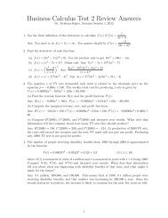
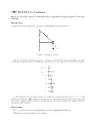
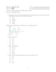
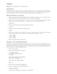
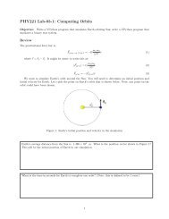
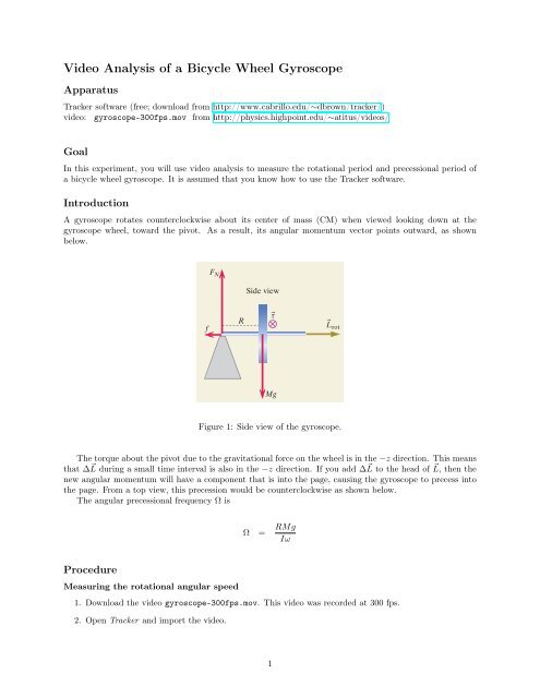
Figure 11.63 Side view showing externalforces acting on the gyroscope and therotational angular momentum vector.There is a torque around the center ofmass, into the page, due to the F N force.WτL rotciple for the gyroscope?The remaining element we need for the Angulartorque that acts around the center of mass, at theLook again at the force diagram (Figure 11.63), andof the torque about the center of mass is RF N =the torque is into the page. Seen from above, the tto the rotational angular momentum (Figure 11.Momentum Principle yields∣d ⃗L rotdt∣ = L rot = τ CMView from aboveFigure 11.64 View from above, showingthe torque vector and the rotationalangular Figuremomentum 2: Top view vector. of the gyroscope.whereL rot = Iω, and τ CM = RMg. Solving for thewe have = τ CM= RMgL rot IωThis is a surprisingly simple result for such a compat least qualitatively with observations. A smallerlarger precession rate .Conversely,agyroscopetvery slowly. If possible, your instructor will providtheory quantitatively by observing an actual gyrossion rates can be measured.3. Open the Clip Settings window by clicking on the Clip Settings icon (shown in Figure 3) which ispart of the video control toolbar that is below the video clip.*ReflectionReflect on how we arrived at this result. Look okey point is that the rotational angular momentumvarying in magnitude, and the magnitude of the ratFigure 3: The Clip Settings icon.angular momentum is simply times L rot .Thisratangular momentum is equal to the net torque actincenter of mass).4. In the Clip Settings pop-up window, enter a frame rate of 300 fps, as shown in Figure 4Figure 4: The Clip Settings icon.REVISED5. A meterstick is shown in the first frame of video. Use this to calibrate distance in the video.6. Since there are 300 frames of video recorded per second, the time interval between frames is quitesmall. As a result, we can skip frames between marking the ball and thus take fewer data points. Clickon the Step Size button, as shown in Figure 5 and change it to 5.Figure 5: Change the step size in order to skip frames.7. Step forward to the first frame that the wheel is rotating. Place the origin at the axle (at the centerof the closest white disk at the hub of the wheel in the video).8. Click the Create button in the toolbar and create a new point mass.2

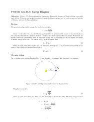
9. Advance to the first frame that the wheel is rotating. Hold the shift key down and click once on thegreen sticker that is on the bicycle tire. The video will then advance 5 frames. Continue to mark thegreen sticker for a total of at least 3 revolutions. If you are only displaying the last few marks, then itwill look something like Figure 6.Figure 6: Marks for the green sticker on the rotating bicycle.10. Right-click on the x vs. t graph and select Analyze .11. Click the button Fit Builder... , click the button Clone , and select “Sinusoid.” In the Fit Builderwindow, add a parameter d with value 0 and add a function a ∗ sin(b ∗ t + c) + d, as shown in 7. Theadditive constant will shift the curve fit up and down by a constant.Figure 7: The Fit Builder is used to fit a curve to a user-defined function.12. Close the Fit Builder window.3

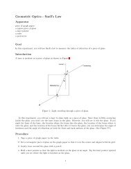
13. You will need to adjust each parameter manually in order to fit a curve to x vs. t. It helps to startwith some reasonable values. So make some approximate guesses for the following functions based onthe curve:a is the maximum value on the curve. What is approximately the maximum value of x?b is the angular velocity, 2π/T . What is the approximate period of the oscillation? Use it tocalculate an approximate value of b.c is the phase. It shifts the curve right or left. You can adjust this manually without knowing theinitial value.d shifts the curve up or down. It should be small, less than 0.01.If you begin with approximate values, you can click in the Parameter Values box and click the upand down arrows to make small adjustments. You can also change the step size as you hone in onthe best value for the parameter.An example curve-fit is shown in Figure 8.Figure 8: The best-fit curve for a point on the wheel.What are the curve parameters and the fit equation for the best-fit curve?4

From the curve fit, determine the radius of the wheel R wheel and the angular velocity ω of the wheel.How does your result compare to the actual radius of the wheel which is 30 cm?Measuring the precessional angular speed1. Start a new Tracker file and import the same video.2. Calibrate the distance just like you did before.3. Now, play the video all the way through and observe the precessional motion of the wheel. We wantto measure the precessional period and frequency.Through how many revolutions did it precess?4. Change the video slider to when the wheel has precessed half a revolution (so that the string is in frontof the plane of the wheel).5. Set the origin of the coordinate system at the center of the white disks.6. Click the Create button and add a point mass.7. Mark the center of the white disk.8. Play the video until the wheel has turned exactly 1/4 of a revolution. Mark the outer white disk (theone furthest to the left). This is the disk that we will track throughout its motion.9. Play the video until the wheel has turned another 1/4 of a revolution. Now, the white disk is furthestto the right. Mark this disk.10. Continue marking this disk for a total of 2 revolutions of the wheel.11. Right-click the graph of x vs. t for mass B and select Analyze . Create a sinusoidal function of theform x = a ∗ siin(b ∗ t + c) + d and adjust the curve fit parameters manually until you get a decentcurve fit. Then, select the checkbox for Autofit. It helps to turn off the “connect the dots" feature byclicking on the line style icon in the datatable. The resulting curve fit may look something like Figure9.5

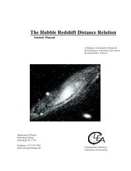
Figure 9: The best-fit curve for the precessional motion of the disk.Approximate the period by taking the time of the last data point and subtracting the time for thefirst data point. Then, use T = ∆t/N where N is the number of revolutions during this time intervalto calculate the period. Using this method, what is the period?What is the equation and fit parameters for the best-fit curve?What is the precessional angular velocity?What is the period (as measured from the precessional angular velocity?6

Compare this result for the period to what you found by calculating T = ∆t/N where N is thenumber of revolutions during the time interval. It’s probably best to report the period found fromthe curve fit, if you are reasonably satisfied that the curve fit indeed fits the data.From the curve fit, determine the radius of precession for this particular white disk. Note that ifthe video were not so dark, we could measure this more precisely on the video itself using the “tapemeasure” tool. However, it can also be easily measured on the wheel itself, as shown below.We really want to calculate the radius of precession from the point of support (the string) to the centerof mass of the wheel. An end view of the axle and hub is shown in Figure 10.9.5 cm11.3 cmFigure 10: A side view of the axle and hub when the plane of the wheel first faces the camera.Using the picture in Figure 10, calculate the radius of precession.7

From your graph of x vs. t for the outer white disk, you determined the distance from the outerwhite disk to the string. Compare your result to what you measure from the picture shown in Figure10. Explain the discrepancy in your results.8