Lab Manual 2005

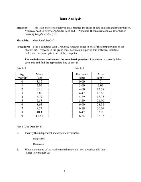
Data AnalysisSituation: This is an exercise so that you may practice the skills of data analysis and interpretation.You may need to refer to Appendix A, B and I. Appendix B contains technical informationon using Graphical Analysis.Materials:Graphical Analysis.Procedure: Find a computer with Graphical Analysis either in one of the computer labs or thephysics lab. Everyone in the group must become an expert in this software, thereforemake sure everyone gets a turn at the computer.Plot each data set and answer the associated questions. Remember to correctly labeleach axis and find the appropriate line of best fit.Data Set 1 Data Set 2Age(months)Mass(kg)Diameter(cm)Area(cm 2 )0 3.17 0.00 01 4.07 3.00 7.072 5.10 4.00 12.573 5.88 4.47 15.854 6.77 4.89 18.755 7.55 5.29 21.996 8.63 6.00 28.317 9.24 6.19 30.098 10.1 6.47 32.909 11.61 6.84 36.75Part 1 (Use Data Set 1)1. Identify the independent and dependent variables.Independent: _______________________Dependent: ________________________2. What is the name of the mathematical model that best describes this data?(Refer to Appendix A)- 1 -

3. Develop a specific physical equation that describes this data.4. Considering delta notation, write a sentence that describes what the slope represents.5. Evaluate the y-intercept with the 5% rule. Is this a zero intercept?6. Explain what the y-intercept represents.7. Develop a general physical equation that describes this data.8. Using both the graph and the specific physical equation, determine the mass at age 4.5months. Was this found by interpolation or extrapolation?9. Using both the graph and the specific physical equation, determine the mass at age 360months. Was this found by interpolation or extrapolation? [Manual scale the graph,x: 0→ 400, y: 0→ 500 ]10. What do you think about the reliability of your answers in questions 8 and 9? Explainyour position.- 2 -

Part 2 (Use Data Set 2)1. Identify the independent and dependent variables.Independent: _______________________Dependent: ________________________2. What is the name of the mathematical model that best describes this data?(Refer to Appendix A)3. Develop a specific physical equation that describes this data.4. Develop a general physical equation that describes this data.5. How can this data be linearized?Linearize the data before answering the remaining questions in this section.6. Develop a specific physical equation for the linearized data.7. Evaluate the y-intercept with the 5% rule. Is this a zero intercept?8. Develop a general physical equation for the linearized data.- 3 -

9. Compare the general physical equation found in question # 8 to that found in #4. How dothey compare? Which method is clearer or easier?10. A well known mathematical formula was used to create Data Set 2. Therefore it can beproven that the slope of the linearized graph represents a known mathematical constant.Determine the mathematical constant that the slope represents by examining the specificphysical equation of the linearized graph (#6) and comparing it with other knownequations. (Consider geometry and the variables which are being examined.)- 4 -

Kinematics(ULV)Situation: Consider driving on a long and straight section of highway using cruise control.We could describe this as motion with a steady pace. (The speedometer always readssome steady value.)Now consider starting a car from a stoplight. How does this motion differ fromcruising along the Trans-Canada? Is stopping a car at a red light fundamentally differentfrom starting? Here we are dealing with an object whose speed is steadily changing.The general purpose of this lab is to formally describe the different types ofmotion. We are concerned with a description of “how” the object moves and are notconcerned with “why” it moves.Materials:A motion detector, metre stick, tractor, track, MPLI and Graphical Analysis.Model 1 (Uniform Linear Velocity)Purpose:To find a mathematical model that describes the relationship between position andtime, for all objects with steady (pace) motion.Procedure:• Enter MPLI and open a file called “Kinematics.exp”. (For more information on usingMPLI see Appendix C.) Plug a motion detector into channel A on the MPLI box andcalibrate the motion detector following the instructions in Appendix C (Calibration mayhave been completed by demonstrator.)• To collect your data, place the tractor in front of the detector. Clear the surroundingarea of possible reflectors. Turn on the tractor and hold it in place at 40 cm from themotion detector (start line).• Have your partner click start on the computer and release the tractor when you hearthe motion detector collecting data. It is not necessary to stop the data collection, it stopsautomatically at the end of the specified time interval.• When the data collection is complete, draw a line of best fit for the graph.→ click on Analyse in the pull down menu. Select Automatic Curve Fittingand choose the model that best represents your graph (see Appendix A).Remember, if the trend is horizontal use statistics.Have your graph checked by an instructor. When you are given the OK, print the graph.- 5 -

Analysis:1. Record the slope and y-intercept of the position -time graph.m = b =2. Using delta notation, determine the general meaning of the slope of the position-timegraph.3. Determine the general meaning of the y-intercept of the position-time graph.4. Develop the specific and general equations for the position-time graph.• Using the tangent and examine buttons, find the slope of the line of best fit at five arbitrarytime instants. This slope is called the instantaneous velocity. Record this data in the tableprovided.Arbitrary Instants Instantaneous Velocity Time1 st2 nd3 rd4 th5 th• Once all the data has been recorded, minimize MPLI and open Graphical Analysis. Plot thedata collected and find the line of best fit.5. The slope of the velocity-time graph should be zero or very close to this. What does thisimply about the motion?6. Determine the general meaning of the y-intercept of the velocity-time graph.- 6 -

7. Calculate the area under the velocity- time graph, from t 2 to t 5 . (Note: The notation t nrepresents the value of t for the n th arbitrary instant.)8. What does this area represent?9. How can you verify this interpretation using the position-time graph?- 7 -

- 8 -

Kinematics(ULA)Situation: Consider driving on a long and straight section of highway using cruise control.We could describe this as motion with a steady pace. (The speedometer always readssome steady value.)Now consider starting a car from a stoplight. How does this motion differ fromcruising along the Trans-Canada? Is stopping a car at a red light fundamentally differentfrom starting? Here we are dealing with an object whose speed is steadily changing.The general purpose of this lab is to formally describe the different types ofmotion. We are concerned with a description of “how” the object moves and are notconcerned with “why” it moves.Materials:A motion detector, metre stick, dynamic cart, track, MPLI and GraphicalAnalysis.Model 2 (Uniform Linear Acceleration)Purpose:To find a mathematical model that describes the relationship between distance andtime, for all objects with steadily increasing motion.Procedure:• Enter MPLI and open a file called “Kinematics.exp”. Calibration may have beencompleted by demonstrator.• The simplest way to get an object to increase (or decrease) its speed at a “steady” rateis to allow it to roll freely down (or up) an incline. We will use the collision cart rolling onour track as the object and use the motion detector with the MPLI to collect our data.• Set up the track with a slight incline. Place the detector at the high end and point it atthe cart. Clear the surrounding area of possible reflectors. To collect data, place your cart40 cm in front of the detector (start line).• Click on the start button and allow your object to roll down the track. Try a fewpractice runs before collecting the data. The trick is to release the cart as you hear themotion detector begin to click.• When the data collection is complete, draw a line of best fit for the graph.→ click on Analyse in the pull down menu. Select Automatic Curve Fittingand choose the model that best represents your graph (see Appendix A).Remember, if the trend is horizontal use statistics.Have your graph checked by an instructor. When you are given the OK, print the graph.- 9 -

Analysis:1. Develop the specific equation for the position-time graph.• Using the tangent and examine buttons, find the slope of the line of best fit at five arbitrarytime instants. This slope is the instantaneous velocity. Record this data in the table provided.Arbitrary Instants Instantaneous Velocity Time1 st2 nd3 rd4 th5 th• Once all the data has been recorded, minimize MPLI and enter Graphical Analysis. Plot thedata collected and find the line of best fit.2. Record the slope and y-intercept of the velocity-time graph.m = b =3. Using delta notation, determine the general meaning of the slope of the velocity-timegraph.4. Determine the general meaning of the y-intercept of the velocity-time graph.5. Develop the general and specific equations for the velocity-time graph.6. Calculate the area under the velocity- time graph, from t 2 to t 5 . (Note: The notation t nrepresents the value of t for the n th arbitrary instant.)- 10 -

7. What does the area represent?8. How can you verify this interpretation using the position-time graph?9. Write the general physical equation for the position-time graph. (Compare specific valuesof coefficients in question #1 and #5 to determine physical meanings of the A, B and Ccoefficients.)10. Based on the velocity-time graphs obtained for both models, sketch the resultingacceleration-time graph.Model 1 (ULV)Model 2 (ULA)vvttaatt- 11 -

KinematicsConclusion:Make a concise summary of the properties of the graphs from the motion studied in bothmodels. Include tiny sketches, general equations, meanings of slopes, intercepts and areas.type of motion properties of x-t graph properties of v-t graphConstant velocity- travelling with“steady” (unchanging)paceSlope =Y int =General Eqn =Slope =Y int =Area =General Eqn =Constantacceleration- travelling with“steadily” changing paceSlope =Y int =General Eqn =Slope =Y int =Area =General Eqn =From now on we will refer to steady paced motion as Uniform Linear Velocity (ULV) andsteadily changing pace motion as Uniform Linear Acceleration (ULA).Briefly sum up the results of this lab.a. In your own words, state what it means to travel with constant acceleration andconstant velocity.b. Explain how to calculate velocity based on a position -time graph.c. Explain how to calculate acceleration based on a velocity-time graph.d. Explain how to get displacement from a velocity-time graph.e. Comment on any errors affecting your results.- 12 -

Projectile SimulationSituation: Projectile motion is simply a case of simultaneous motion in two directions. Weneed to assess the motion in each direction.Theory: Divide and conquer. Analyzing what happens in two directions simultaneously isdifficult for us to do. However, if we can look at the vertical motion seperately from thehorizontal motion, then we have a chance at interpreting this event.Procedure: To aid in the study of projectile motion we will use a program called WorkingModels 3.0.3 which will allow us to create and launch our own model. As well, the programwill allow us to analyse the resulting two-dimensional motion map. The followinginstructions will help you create your own motion map.→ Open Working Model 3.0.3 and maximize the window.→ To create a reference frame for the motion of the object we need a co-ordinate system→ enter View → Workspace → XY Axes→ enter View → Workspace → Gridlines→ To create an object click the circle located on the toolbar (about the third down), returnto the screen and “click and drag”. Try not to create an object that is to big because itbecomes more difficult to track.→ Now we need to move our object to the origin and give it an initial velocity.→ scroll down until the origin of the XY axes is in the lower left corner of thewindow→ double click on the object so that a “properties” window appears→ set the x and y co-ordinates to 0 m. (Note that the object is now positioned at theorigin)→ give the object an initial velocity by setting the horizontal and verticalcomponents. (Try v x = 5 m/s and v y = 7 m/s)→ close the properties window→ Now we need to track the motion of the projectile→ enter World → Accuracy→ in the box that appears change the animation step from the Automatic to 0.1s→ enter World → Tracking → every frame→ enter Measure → Time- 13 -

→ To measure the exact position of the projectile it is necessary to create a position box→ click on the object→ enter Measure → Position →All→ in the Position box that appears click on “rot” to turn it off. This measurement isnot required since our object has no rotation.→ We are now able to run the simulation and track the path taken.→ click RUN (note: the RUN button will change to a STOP button once started)→ after approximately 2.0s stop the motion and hit RESET→ In the bottom left corner there appears a tracking deviceBrings the objects back to the starting position (rewind)Run the objects through the motion againAdvances the motion frame-by-frame (slow motion)Rewinds the motion frame-by-frame→ Advance the motion frame-by-frame by clicking→ Collect the data required to analyse the motion. The x-axis represents the horizontalmotion and the y-axis represents the vertical motion.→ keep in mind that the time for each point occurred at 0.100s intervals→ record the x and y position of each point by advancing frame-by-frame andreading the co-ordinates from the position box.→ record all values in the data table provided.→ Once all data has been collected minimize Working Models and enter GraphicalAnalysis.→ open a file marked “projecti.dat” (this contains a template of the necessarygraphs)→ plot the position-time and velocity-time graphs for the horizontal and verticalaspects of motion. You will obtain four graphs in all, two for horizontalmotion and two for vertical motion.→ Remember to use the curve fitting options to obtain a line of best fit for eachgraph.- 14 -

DATADot # Time (s) Horizontalx (m)0123456789101112131415Verticaly (m)Analysis:1. Determine the specific physical equation for each graph. Use appropriate symbols foreach equation.Position x vs. time :Velocity x vs. time :Position y vs. time :Velocity y vs. time :- 15 -

2. What motion model (ULV or ULA) applies to the horizontal motion? How do you know?3. What motion model applies to the vertical motion? How do you know?4. Referring to the appropriate graphs:a) Determine the initial horizontal speed. How did you get this value?b) Determine the initial vertical speed. How did you get this value?5. Using the values from question 4, calculate the launch velocity. Include a tip-to-taildiagram and express the final answer in the form magnitude (units) @ degrees to thehorizontal.6. Use vector addition to determine the velocity at 0.300s.7. What should v y be at maximum height?8. Determine the velocity at the maximum height.9. What is the velocity at 1.5s ?- 16 -

10. What is the velocity at 2.0s ? Show your workings. [Use the appropriate equationsdetermined in question 1.]11. What is the ball’s vertical and horizontal position at 2.0s ? Show your workings. [Use theappropriate equations determined in question 1.]12. A golfer on Gros Morne drives golf balls off the peak at 14.0 m/s @ 20° above thehorizontal. If the peak is 800m above the bottom of the Fjord on the north side of themountain, then determine the ball’s:a) time of flightb) horizontal rangec) maximum altitude of the ball (relative to the Fjord)d) impact velocity13. A ping pong ball bounces off a table, 0.85m above the ground. If the ball strikes the floorat 5.44 m/s @ 56.5° below the horizontal, then determine the ball’s:a) initial velocityb) time of flightc) horizontal ranged) maximum height relative to the floor- 17 -

- 18 -

Relative Velocity SimulationSituation: Consider two ships at sea that are travelling near each other. The radar operator onone ship can see the other ship on his radar screen. With each sweep of the radar it plotsthe position of the other ship relative to his ship. His ship is located at the center of thescreen. From this information he can easily tell the rate at which the ship is approachinghim. This is known as relative velocity.But does this tell us the other ships actual speed? Does it tell us the actualdirection the other ship is headed? This lab exercise will attempt to give you anunderstanding of the concept of relative velocity and how it relates to actual velocity.Frames of Reference1. Suppose you are on a ship that is moving “forward”. When you look over the side at thewater, which way does it appear to move? (Consider the speed of the water flow and thedirection in comparison to the speed of the ship itself)2. What if you were restricted to only looking at the water flowing along the side of theship? Do you think this observation could accurately give you information about themotion of the ship?3. Suppose you were on a ship that was anchored in the middle of a river, where the currentis very fast. You look over the side and observe the water flow around the ship. Whatdoes it look like?4. Re-examine your answer to question 2. Make any additional comments here.5. Have you ever had your car stopped at a traffic light and noticed the car ahead of you rollback toward you. Did you briefly get the sensation that you are actually moving insteadof the car ahead? While this sensation is happening is there any way of determining forsure who is actually moving?6. Now suppose that in question 5 you are not stopped at a light but are parked on a ferryand as the ferry begins to pull out from the dock the car ahead of you, which wasmistakenly left in neutral, starts approaching you. Compare this situation with question5. Which car is now moving? Is it possible to tell from your observations?- 19 -

Part 1:One Dimensional Relative VelocitySituation: To study one-dimensional relative velocity we will use Working Models tocreate a motion map representing two ships travelling in the same direction along thesame linear path.→ Open Working Models and maximize the screen.→ In order to view the entire motion of our simulation we can now set the width of ourwindow.→enter View → View Size → Window Width → 25 m→ We will first need to create the objects used in the simulation. To make thesimulation easier to follow we will create two different types of objects (onerectangular and one circular) of approximately the same size.→ from the toolbar along the left side of the window click on the circle.→ return to the window and "click and drag" to create a circle.→ from the toolbar along the left side of the window click on the rectangle.→ return to the window and "click and drag" to create a rectangle.→ We will now have to set the initial properties of each object. Keep in mind that the twoobjects will be travelling along the same linear path.→ Double click on the rectangular object .→ In the properties window that appears set the position and the velocity by changing tothe following co-ordinates x = -4.0 m, y = -2.0 m, v x = 3.0 m/s, and v y = 0 m/s.→ In the pull down menu of the Properties window select the circular body (note thatthe circular object now becomes highlighted).→ We can now set the position and velocity of the circular object by changing to thefollowing co-ordinates x = -1.0 m, y = 1.0 m, v x = 2.0 m/s, and v y = 0 m/s.→ Close the Properties window and note that the circular object should now be aboveand slightly to the right of the rectangular object.→ For our simulation we would like to create a “Bird’s Eye View”. Essentially, thismeans that we would like to observe the motion of the objects as seen from above.To accomplish this we must turn the gravity off.→ enter World → Gravity → None→ It is also useful to have the XY axes as a reference frame for the motion→ enter View → Workspace → XY Axes→ Note that since our view of the simulation occurs from above, the XY axesnow acts as a compass where the Y axes represents the North-South axes andthe X-axes represents the East-West axes.→ Throughout our simulation it will be necessary to measure the exact position of eachobject.→ Click on the rectangular object.→ Enter Measure → Position → All- 20 -

→ It is also convenient to have velocity vectors which indicate the magnitude anddirection of the velocity.→ Enter Define → Vectors → Velocity→ Click on the circular object and repeat the previous steps.→ In the Position box that appears click on “rot” to turn it off. This measurement is notrequired since our object has no rotation.→ Move Position boxes to a more convenient location by clicking on the title anddragging the box.→ It will also be necessary to record the time of the motion as we run our simulation.→ Enter World → Accuracy→ Change the Animation Step to 0.100 s and click OK.→ Enter Measure → Time→ We are now able to measure the exact position of the two objects throughoutthe run.→ To run the simulation click the RUN button located in the upper left corner (note: TheRUN button becomes a STOP button once activated.)→ After approximately 6 s stop the simulation (click STOP).→ We are now able to collect data regarding the separation displacement between the twoobjects.→ In the bottom left corner there appears a tracking deviceBrings the objects back to the starting position (rewind)Run the objects through the motion againAdvances the motion frame-by-frame (slow motion)Rewinds the motion frame-by-frame→ Click RESET to return to the start of the motion.→ Advance the motion frame-by-frame by clicking→ For every 5 frames record the horizontal separation displacement (x c – x r ) and thetime. [Note: We are using the “rectangle” ship as our reference object. That is, all ofour measurements are taken from the rectangle’s position.]Horizontal Separation Displacement(x c – x r )Time (s)- 21 -

Analysis:1. Suppose you were on the bridge of the ”rectangle” ship. According to your observation,how and in which direction does the other ship appear to be moving? (Consider how theseparation displacement is changing with time.)2. Suppose you were on the “circle” ship instead. How would the motion of the “rectangle”ship appear? (Consider both magnitude and direction.)→ To check your answers for #1 and #2 return to the simulation. It is possible torun the simulation while using one of the objects as a frame of reference. Thatis, the simulation will now be seen from the point-of-view of the chosenobject.→ click on the "rectangle" ship→ enter View → New Reference Frame → (the object name shouldappear and the "show eyeball" should be turned on) → click Ok→ run the simulation and note that the rectangle now appears fixedwhile the circle and XY axes are in motion.→ repeat for the "circle" ship→ to return to the original reference frame enter View → Home→ to reset the window widthenter View → View Size → Window Width → 25 m3. What is the separation displacement between the ships at the following time intervals?t = 0 st = 1.0 st = 3.0 st = 5.0 st = 7.0 s→ Minimize Working Models and enter Graphical Analysis. Plot a graph of separationdisplacement vs. time.- 22 -

4. Considering delta notation, determine the general meaning of the slope of the position -time graph.5. What is the numerical value for the rate of change of separation displacement?6. What can you say about how the separation displacement is changing?7. Considering the initial velocities of each object, could the rate of change of separationdisplacement be determined indirectly (without measurement from motion maps)?V c = _________V r = _________8. Now suppose that the same two ships are again travelling on the same path, but inopposite directions, with the same speeds as they had before. Imagine you are on the“rectangle” ship but this time the “circle” ship is ahead of you and heading towardsyou. How would you determine the relative velocity of the circular ship?Part 2:Two Dimensional Relative VelocitySituation: We will now use Working Models to examine the situation where twomoving objects, such as our two ships, are travelling in a straight line but notalong the same path.→ Open Working Models by clicking on the minimized Working Models window (located nextto the start button).→ Since we are entering back into the previous simulation the environment set-up willbe the same and we will only need to change the property settings of each object.- 23 -

→ We will now have to set the initial properties of each object. Keep in mind that the twoobjects will not be travelling along the same linear path.→ Double click on the rectangular object.→ In the properties window that appears set the position and the velocity by changing tothe following co-ordinates x = -1.0 m, y = -5.0 m, v x = 2.0 m/s, and v y = 1.5 m/s.→ In the pull down menu of the Properties window select the circular body (note that thecircular object now becomes highlighted).→ We can now set the position and velocity of the circular object by changing to thefollowing co-ordinates x = -5.0 m, y = 2.0 m, v x = 2.5 m/s, and v y = -1.0 m/s.→ Close the Properties window and note that the circular object should now be aboveand slightly to the left of the rectangular object.→ To run the simulation click the RUN button located in the upper left corner (note: TheRUN button becomes a STOP button once activated.)→ After approximately 6 s stop the simulation (click STOP).→ Objects should not collide. If a collision occurs, check co-ordinates and object size.→ We are now able to collect data regarding the separation displacement between the twoobjects.→ Click RESET to return to the start of the motion.→ Advance the motion frame-by-frame by clicking→ For every 5 frames record the horizontal separation displacement (x c – x r ), verticalseparation (y c – y r ), and the time. [Note: We are using the “rectangle” ship as ourreference object. That is, all of our measurements are taken from the rectangle’sposition.]Time (s)Horizontal Separation Displacement(x c – x r )Vertical Separation Displacement(y c – y r )→ Once all data has been collected minimize Working Models and enter GraphicalAnalysis.→ In Graphical Analysis plot a displacement vs. time graph for both the horizontaland vertical components. Do not forget to use the curve fitting options.- 24 -

Analysis:1. What does the slope of each graph represent?2. Calculate the velocity of the “circle” ship with respect to the “rectangle” ship in this 2-Dsituation as you did in the 1-D situation. [Hint: Consider vector analysis.]3. Suppose you were on the bridge of the ”rectangle” ship. According to your observation,how and in which direction does the other ship appear to be moving? (Consider how theseparation displacement is changing with time.)4. Suppose you were on the “circle” ship instead. How would the motion of the “rectangle”ship appear? (Consider both magnitude and direction.)→ To check your answers for #3 and #4 return to the simulation. It is possible torun the simulation while using one of the objects as a frame of reference. Thatis, the simulation will now be seen from the point-of-view of the chosenobject.→ click on the "rectangle" ship→ enter View → New Reference Frame → (the object name shouldappear and the "show eyeball" should be turned on) → click Ok→ run the simulation and note that the rectangle now appears fixedwhile the circle and XY axes are in motion.→ repeat for the "circle" ship→ to return to the original reference frame enter View → Home→ to reset the window widthenter View → View Size → Window Width → 25 m- 25 -

5. Using the initial velocities assigned to each object, the velocity of each ship can bedetermined to be:Velocity of “rectangle” ship 2.5 m/s @ 36.9° N of E ..Velocity of “circle” ship 2.7 m/s @ 21.8° S of E .Magnitude θ θ standard x-component y-component2.5 36.9º N of E V xr = V yr =2.7 21.8º S of E V xc = V yc =V xc - V xr = V yc - V yr =Vector DifferenceFind the vector difference between the velocities of the two ships.6. Compare the answers found in questions #2 and #5. What conclusion can now be maderegarding relative velocity?- 26 -

Constant Net Force ModelSituation: At the heart of dynamics is the notion of net force. The constant net force modelsays that when the net force on an object is non zero (F net ≠ 0), then the objectundergoes constant acceleration.EX 1: Consider two identical cars stopped on a level road at a stoplight. The driver of car A isvery aggressive and will press the gas peddle to the floor when the light turns green. CarB’s driver is more cautious and will only press the gas peddle a quarter of the way down.Both drivers press on the gas as soon as the light changes.What type of motion will each car have after the light changes colour?What dynamic model applies to each car?How might the motion of each car differ? Explain how and guess why this is so.What variables might be displayed here? Which could be independent and which should bedependent? What factor seems to be held constant?EX 2: Now consider this. Two identical tractor trailers are stopped at the same intersection asabove. Both drivers are equally aggressive and will press on the gas all the way when thelight turns green. However, one truck is fully loaded with 2 tonnes of steel pipes and theother is completely empty.What type of motion will each truck have after the light changes colour?What dynamic model applies to each truck?How might the motion of each truck differ? Explain how and guess why this is so.What variables might be displayed here? Which could be independent and which should bedependent? What factor seems to be held constant?- 27 -

Materials:Theory:A motion detector, a force sensor (mounted on a dynamic cart), dynamic cart andtrack, string, mass set, MPLI and Graphical Analysis.Before we continue with the experiment draw a semi scaled FBD and VCD, of adynamic cart with uniform linear acceleration on a level track.cartfrictionlessmWhat assumptions have you made about the forces acting on the cart?Purpose:To find a mathematical model that explains the relationship between net force,mass and acceleration, for all objects with uniform linear acceleration.Procedure:• It should be clear that the rate at which you accelerate may be effected by morethan one variable. The apparatus we recommend you use, should work for all thenecessary tests.• Enter MPLI and open the file called “Newton.exp”. A F vs. t and a v vs. t graphshould appear which will allow us to collect our data.• Next you must calibrate the force sensor and motion detector (see Appendix C).(Calibration may have been completed by demonstrator.) Make sure that when calibratingthe force sensor that the cart does not move and that the sensor is arranged in the way itwill be used.• Since we have two independent variables we must run two tests to see how thevariables are related to the dependent variable. For each test, one variable must be heldconstant while the other variables are being examined.- 28 -

Part 1: Vary the force applied while keeping the mass of the cart constant.→ Record the mass of the cart (include the mass of the attached force sensor).m = ______________ kg→ To vary the force applied, change the mass attached to the string. Vary the mass from20g to 300g. For each trial record the mass attached and collect data.→ Place the cart 40 cm from the motion detector (at start line). Attach a mass to the endof the string and place string over frictionless pully.→ Have your partner click start on the computer and release the cart when you hear themotion detector collecting data.→ Collect the required data and repeat procedure for new attached mass (force).→ record the force applied from the force-time graph [Remember if the trend ishorizontal to use statistics and obtain the average value.]→ record the acceleration from the velocity-time graph→ Record all data in the table provided.Part 2: Vary the mass of the cart while keeping the force applied constant.→ Calculate and record the applied force using the equation given. ( m C is the mass ofthe cart and m H is the mass attached to the string.)FT=mmC Hgm + mCHF T = ______________ N→ Vary the mass of the cart, in 100g increments, by placing masses on top of the cart.Include the initial mass of the cart in all measurements.→ Place the cart 40 cm from the motion detector (at start line). Attach a 50g mass to theend of the string and place string over frictionless pully. Place mass on top of cart.→ Have your partner click start on the computer and release the cart when you hear themotion detector collecting data.→ Collect the required data and repeat procedure for new cart mass.→ record the acceleration from the velocity-time graph→ Record all data in the table provided.For each experiment do 7-10 trials. Record the data in table provided.- 29 -

Part 1 Part 2Attached Force (N) AccelerationMass of CartMass (kg)(m/s 2 )(kg)Acceleration(m/s 2 )When you have collected the data for all experiments, minimize the MPLI program and enterGraphical Analysis.→ Plot the data for each experiment. An acceleration vs. Force graph (for Part 1) andacceleration vs. mass of cart graph (for Part 2) should be obtained.→ Remember to use the curve fitting options to obtain a line of best fit for each graph.Analysis:1. State the proportionalities for both graphs and the joint variation proportionality.2. Determine the average proportionality constant for the joint variation (see Appendix J).What are its units?3. Rewrite the equation for this data.a. Solving for acceleration.b. Solving for force.- 30 -

4. According to 3b what are the units of force? Are these units equivalent to the newton?5. Based on the units given in question 4, describe in your own words what 1N of net forceis.6. Imagine a massless object under the influence of some net force. How much accelerationdoes it have? [By massless we are referring to an object that is so small that it can beconsidered massless but does not have a mass of zero.]7. A student told me that an object’s mass is its resistance to being in motion, ( i.e.,massive objects come to a stop faster than lighter objects). Is this idea correct? Defendyour choice in terms of the graphs you have plotted.8. State two ways to calculate net force.9. Given this scale VCD and that the object has a mass of 2.50 kg, what is its acceleration?How far will the object travel in 5 seconds, if it starts from rest?F N1 cm = 1 NF mF rF g sin θF g cos θ- 31 -

10. An object accelerates at 9.80 m/s 2 with a net force of 123.0 N, what is its mass?11. Given a net force of 15 N on a 1.25 kg cart, what is the acceleration?12. A 60 kg person sits on a level, carpeted floor. If the person is pushed across the floor witha force of 255 N and the friction is known to be 245 N, determine the acceleration of theperson.Conclusions:Briefly sum up the results of this lab.a. Compare the two ways of calculating net force.b. State Newton’s second law in your own words.c. State how are the variables related to each other.d. Discuss any possible sources of error in this experiment.- 32 -

Materials:Purpose:A force sensor, wooden blocks, surface board, mass set, MPLI and GraphicalAnalysis.To find a mathematical model that explains the relationship between weight,normal force, and friction, for all sliding objects.Procedure: We want you to examine the nature of sliding friction. To do this you will pull thewooden block along some surface with a calibrated force sensor. Each group will use adifferent surface combination. For all tests that you might do you must first devise a wayto knowingly measure the sliding friction force. Remember that the force sensor onlymeasures the force you supply to pull the object.When pulling the block, what type of motion should you strive for? Justify in terms of yourdynamic models? Draw a semi scale FBD and VCD.• Enter MPLI and open the file called “Friction.exp”. A F vs. t graph should now appear. Nextyou must calibrate the force sensor (see Appendix C). Make sure that when calibrating the forcesensor, it is arranged in the way it will be used.• In this experiment we will vary the normal force (by adding mass to the block) and recordboth the kinetic and static friction.• Where possible do several trials using different values of the normal force. Remember to pullthe block with constant velocity, starting from rest with no tension in the string.• Record all data in the table.→ calculate the normal force→ record the value of friction when the object was moving (kinetic) and the maximumvalue of friction before the object started to move (static) from the Force- time graph.Combined mass ofblock and attachedmass (kg)Normal Force (N) Static Friction (N) Kinetic Friction (N)- 34 -

• When you have collected the data, minimize the MPLI program and enter Graphical Analysis.Plot the data for each experiment. On the same graph plot maximum efforts to start moving (f s )and average effort to keep moving (f k ) vs. the normal force.Analysis:1. Based on the pre-lab questions, which factor is best linked with friction, Normal Force orWeight?2. State the nature of the relationship between friction and the normal force.3. Develop the general and specific equation of both the static vs normal force and kineticvs. normal force graphs.4. What is the value and general meaning of the slope of your friction vs. normal forcegraph. (Consider unit analysis.)5. When friction is involved, does it take more force to start motion then it does to keepmoving? What does this say about the nature of friction?6. Air resistance is another form of friction. Move your arm through the air with a lowuniform velocity. Now imagine if your arm is stuck out of the window of a car moving at100 km/h. When does air resistance feel stronger? What does air resistance depend on?Would our model of sliding friction apply to explain air friction? Explain.- 35 -

7. Given that two objects of equal mass and surface texture but different contact areas, aresliding across the same surface with constant velocity, which is true:a. The block with greater contact area feels a larger frictional force.b. The block with smaller contact are feels a greater frictional forcec. Both block feel equal fictional force(Justify your choice. Try examining your block using different surface areas.)8. A 3.2 kg block is allowed to slide down a rough but perfectly vertical surface. What is thefrictional force on the block? Explain?9. How much force is required to accelerate a 30 kg block, at 2.5 m/s 2 , along your surface,when it is horizontal? Include a semi scale FBD and VCD.10. What is the frictional force experienced by a 15.0 kg block sliding on your horizontalsurface?Conclusions:Briefly sum up the results of this lab.a. What factors govern the nature of sliding friction?b. What factors determine the magnitude of friction? What ones do not?c. State differences in static and kinetic friction.d. Discuss any sources of error which may have occurred.- 36 -

Circular MotionSituation: Consider an object like a rubber ball tied to a piece of string being swung in ahorizontal circular path at a constant speed.Is this type of motion natural? That is, if the string broke would the ball continue in itscircular path?What is the string doing to the ball that causes it to move the way it does?Predict how changing the ball’s mass will affect the tension in the string?Predict how changing its speed will affect the tension?Predict how changing the radius of the path will affect the tension?Theory: Objects moving in a circular path require a force, known as the centripetal force,to keep the object moving along that path. Centripetal force is a center seeking force. Themagnitude of the centripetal force is affected by the object’s speed, mass, and the radiusof the circle in which the object is travelling.Purpose: We would like to develop a mathematical model that shows the effect of theobjects speed, the radius of the path, and the mass of the object on the amount of forcerequired to cause it to move in a horizontal circular path.Materials:MPLI, turntable, Force sensor, various masses, and string.Procedure: To develop this model we have designed a turntable that allows you to record theforce while varying the velocity, radius, and mass of the object. However, to successfullydetermine the relationship we must examine the effect that each variable has on the forcewhile the other variables remain constant. Therefore, we have divided the lab into threeparts, where different groups will perform different parts and the information will beshared to obtain the final result.- 37 -

Part 1: Varying the mass.• Enter MPLI and open the file “circular.exp”. This file contains a Force vs. Time graph,which will allow you to record the force, and also contains the necessary calibration.• While varying the mass it is important to keep the radius of the circular path constant.The radius should be measured from the center of the turntable to the center of the object.The radius can be adjusted by moving the force sensor up or down the ring stand. Recordthe radius that you are using.r =• It is also important to keep the velocity of the object constant. Start your turntable usinga gentle push. If the same person starts the motion each time with a steady and consistentforce then the velocity should remain fairly constant. However, there will be somevariation.→ As the object rotates a sin wave appears on the Force vs. Time graph.→ The time required for one complete rotation is the time difference betweensuccessive peaks. Therefore, we can keep the velocity constant by allowing thesweep to run until we have a certain number of waves for each trial (example: 5waves in 5s).→ Once the correct number of waves is reached press stop or the readings willcontinue and the necessary information will be lost. It is important to stop at theend of the sweep.→ We can now calculate the velocity since we know the distancetravelled by the object in one cycle and the time required for that cycle to becompleted. (Note: time for one cycle = time / # of waves, the distancetravelled is equal to the circumference of the circle.)average velocity =• Record the force from the graph by taking the statistical average. Both the force and themass should now be recorded in an appropriate table. Repeat the experiment several timesusing different masses. Determine the mass of your object using the balance provided.Force (N)Mass (Kg)• Once all data has been collected enter Graphical Analysis and plot a graph of Force vs.Mass. Linearize the data to determine how the force and mass are related. Print threecopies of your graph.- 38 -

Part 2: Varying the Velocity.• Enter MPLI and open the file “circular.exp”. This file contains a Force vs. Time graph,which will allow you to record the force, and also contains the necessary calibration.• While varying the velocity it is important to keep the radius of the circular pathconstant. The radius should be measured from the center of the turntable to the center ofthe object. The radius can be adjusted by moving the force sensor up or down the ringstand. Record the radius which you are using.r =• It is also important to keep the mass of the object constant. Record the mass of yourobject using the triple beam balance provided.m =• Start your turntable using a gentle push. By varying the force each time then a differentvelocity should be obtained.→ As the object rotates a sin wave appears on the Force vs. Time graph. The timerequired for one complete rotation is the time difference between successive peaks.→ We can now calculate the velocity since we know the distance travelled bythe object in one cycle and the time required for that cycle to be completed. (Note:time for one cycle = time / # of waves, the distance travelled is equal to thecircumference of the circle.)• Record the force from the graph by taking the statistical average. Both the force and thevelocity should now be recorded in an appropriate table. Repeat the experiment severaltimes using different velocities.Force (N)Velocity (m/s)• Once all data has been collected enter Graphical Analysis and plot a graph of Force vs.Velocity. Linearize the data to determine how the force and velocity are related. Printthree copies of your graph.- 39 -

Part 3: Varying the radius.• Enter MPLI and open the file “circular.exp”. This file contains a Force vs. Time graph,which will allow you to record the force, and also contains the necessary calibration.• While varying the radius it is important to note that the radius of the circular path shouldbe measured from the center of the turntable to the center of the object. The radius can beadjusted by moving the force sensor up or down the ring stand. It is also important thatthe radius start from the smallest and increase at equal increments to the largestobtainable radius.• It is also important to keep the mass of the object constant. Record the mass of yourobject using the triple beam balance provided.m =• It is important to keep the velocity of the object constant. Start your turntable using agentle push. Since the radius of the object’s path is increasing than the time interval foreach reading will also have to increase for the velocity of the object to remain constant.→ As the object rotates a sin wave appears on the Force vs. Time graph. The timerequired for one complete rotation is the time difference between successivepeaks. Therefore, we can determine the time interval by recording the number ofwaves in a certain amount of time (example: 12 waves in 8s).→ For the initial reading, with smallest radius, try to get the table moving asquickly as possible. Keep trying until 12 peaks appear in the 8s time interval. Wecan now calculate the velocity since we know the distance travelled by the objectin one cycle and the time required for that cycle to be completed. (Note: time forone cycle = time / # of waves, the distance travelled is equal to thecircumference of the circle.)→ For each additional reading, the radius will increase. To ensure v is constantfor all trials then we must also increase the time period (T) by the same amount.v = 2πrTguideline:Radius← increase r by a factor of n← increase T by same factor of n* to increase T by a factor of n, we needto change the # of cycles by factors of 1/n.# of cycles in 8s sweepr 1 = 5cm → 12r 2 = 2( r 1 ) = 10cm → ½ (12) = 6r 3 = 3( r 1 ) = 15cm →1 3 (12) = 4r 4 = 4( r 1 ) = 20cm → ¼ (12) = 3r 5 = 5( r 1 ) = 25cm →1 5 (12) = 2.4r 6 = 6( r 1 ) = 30cm →1 6 (12) = 2- 40 -

→For each additional reading, allow the sweep to run until we have the correctnumber of waves for the 8s time frame. Once the correct number of waves isreached record the average force.• Record the force from the graph by taking the statistical average. Both the force and theradius should now be recorded in an appropriate table. Repeat the experiment severaltimes using a different radius each time.Force (N)Radius (m)0.050.100.150.200.250.30• Once all data has been collected enter Graphical Analysis and plot a graph of Force vs.Radius. Linearize the data to determine how the force and radius are related. Print threecopies of your graph.Analysis:Once you have obtained all three graphs (one for each variable) determine theproportionalities for each. You can now determine the joint variance (seeAppendix J) and use your information to calculate the proportionality constant.- 41 -

1. A 25.0 kg child on a merry-go-round is moving with a speed of 1.35 m/s when 2.0 m fromthe center of the merry-go-round. Calculate the net horizontal force exerted on the child.2. A horizontal force of 200 N is exerted on a 2.0 kg disc as it is rotated uniformly in ahorizontal circle of radius 1.0 m. calculate the speed of the disc.3. A 0.40 kg ball, attached to the end of a cord, is rotated in a circle of radius 1.2 m on africtionless horizontal surface. If the cord will break when the tension exceeds 50 N, whatis the maximum speed the ball can have?- 42 -

CollisionsSituation: Have you ever witnessed a car accident? How many different types of collisionhave you seen? Most people have witnessed various types of collisions, either real life ormovie stunts, and can describe different situations. For example, imagine a speeding carcolliding with a parked car. After impact the two vehicles could bounce apart and moveoff at different velocities or they could become entangled and move together at onecombined speed. Now consider a head on collision where the two vehicles, movingtowards each other, stick together after impact and continue with a new velocity.Each of these collisions, although having different conditions before and after impact, canbe analyzed using the same techniques since collisions between objects are governed bythe laws of momentum and energy. In this lab we will examine various collisions usingboth the Law of Conservation of Momentum and the Law of Conservation of Energy.Theory: The Law of Conservation of Energy allows us to analyze initial conditions for asystem and predict conditions and behaviour at a later time. The law states that the energyin a system is constant. However, some energy may be in a form that isn’t easy tomeasure – for instance, frictional heating or the deformation of an object. The Law ofConservation of Momentum provides a simple method for the analysis of systems thatinclude these elusive forms of energy.The Law of Conservation of Momentum states that the total momentum of a system isconstant. Momentum is the “quality” or “durability” of motion. In physics terms,momentum is an object's mass multiplied by its velocity. The symbol for the quantitymomentum is the small case “p”; therefore the equation can be written as:p = m × vIt is important to note that the law of conservation of momentum states that the totalmomentum in a “system” is constant. When we use the word “system”, we mean all ofthe objects we are considering. We could have several objects that interact with eachother, but with nothing else. In that case, one object could transfer some or all of itsmomentum to another object, but the sum of all of the momentum in this system wouldremain the same. However, a force acting for a given amount of time will change anobject's momentum.Put another way, an unbalanced force always accelerates an object - either speeding it upor slowing it down. If the force acts opposite the object's motion, it slows the objectdown. If a force acts in the same direction as the object's motion, then the force speedsthe object up. Either way, a force will change the velocity of an object and if the velocityof the object is changed, then the momentum of the object is changed.- 43 -

These concepts are merely an outgrowth of Newton's 2 nd law. Newton's 2 nd law( F net= m × a ) stated that the acceleration of an object is directly proportional to the netforce acting upon the object and inversely proportional to the mass of the object. Whenv − v0combined with the definition of acceleration ( a = ), the following equalities result.tF Net∆v= mtIf both sides of the above equation are multiplied by the quantity t, a new equationresults.F Nett = m ∆vt = ∆pF NetTo truly understand the equation, it is important to understand its meaning in words. Inwords, it could be said that the force times the time equals the mass times the change invelocity. In physics, the quantity F Net × t is known as the impulse. Since the quantity m×vis the momentum, the quantity m×∆v must be the change in momentum. The equationreally says that theImpulse = Change in momentumIn a collision, an object experiences a force for a specific amount of time which results ina change in momentum (the object's mass either speeds up or slows down). The impulseexperienced by the object equals the change in momentum of the object. During thecollision the two objects are in contact for the same amount of time and exert equal, butopposite, forces on each other (Newton’s 3 rd Law). As a result the total momentum of thesystem is conserved.The system we wish to focus on consists of two dynamic carts that will be used torecreate various types of collisions. In some collisions, objects bounce off of each other.If no energy is used to deform the object (or produce sound or heat), these collisions aretermed elastic collisions. (In other words, if kinetic energy is conserved in a collision,then it is elastic.) In other collisions, objects still bounce, but use some of their energydeforming each other and/or producing sound. These are called inelastic collisions.Sometimes objects stick together during a collision. These are called completely inelasticcollisions. Examples of completely inelastic collisions include throwing silly puttyagainst a concrete wall, colliding a car with a tree, or rolling a dynamics cart into anotherdynamics cart and allowing the velcro on each to stick the carts together.Again the momentum and energy of the system are conserved in all types of collisions.However, the form of the final energy is not always easy to measure. Objects in inelasticcollisions lose kinetic energy to the energy of deformation, sound, or heat. For thisreason, we use the Law of Conservation of Momentum when examining collisions.- 44 -

In the lab, we will measure the velocity of two carts on dynamic tracks using the LabProSoftware for various collisions. From this we can determine their respective momentum.In principle, we could make systems that have more than two cars, but that would justcomplicate the experiment and the calculations. Remember that if the cars bump intoanything, like the ends of the track, momentum is no longer conserved, since the car hasinteracted with something outside the system.Purpose: The principles of conservation of momentum and/or energy are studied for bothelastic and inelastic purposes.Materials:LabPro software, dynamic carts and tracks, vernier motion sensors, balance.Part 1Procedure: The following experiment will be demonstrated by the instructor. Students mustpay close attention and record all data in the table provided.Set up a collision between a dynamic cart and a force sensor. The force sensor willdetermine the force upon impact. Use the statistics option to determine the average forceapplied during contact. Also the duration of the contact (collision) can be read from thetime axis. There is also a column in the table to record the area beneath the F vs t graphfor the duration of the collision.Cartmass v i v f ∆p Ave Force ∆t Impulse AreaAnalysis:1. How does the change in momentum for the cart compare to the impulse?2. What causes the change in momentum for the cart?3. What does the area under the F vs. t graph represent?4. How does the area recorded compare to the impulse?- 45 -

Part 2Procedure: Collisions between freely moving carts are executed on the tracks. Frictionbetween the track and the carts are assumed negligible. The acceleration due to the forceof gravity is eliminated by restricting all motion to the horizontal plane ( i.e., levelling thetrack). The track will be levelled in advance by the lab instructor.Collision:Of six different possible collisions, two or three collisions will be assigned forexamining. For each collision set-up, record the mass of both carts using the balanceprovided.Determine the initial and final velocities for both carts from the graphs obtained andrecord all information in the table provided. An explanation as to how to read from thegraphs will be provided by the lab demonstrator.Cart 1Mass(kg)V i (m/s) V f (m/s) P i(kg m/s)P f(kg m/s)Cart 2Total momentum of Cart 1 and Cart 2(Σ)Compare the initial and final total momentum of the two-cart system.→ Has momentum been conserved? If not, why?Collision:Cart 1Mass(kg)V i (m/s) V f (m/s) P i(kg m/s)P f(kg m/s)Cart 2Total momentum of Cart 1 and Cart 2(Σ)Compare the initial and final total momentum of the two-cart system.→ Has momentum been conserved? If not, why?- 46 -

Collision:Cart 1Mass(kg)V i (m/s) V f (m/s) P i(kg m/s)P f(kg m/s)Cart 2Total momentum of Cart 1 and Cart 2(Σ)Compare the initial and final total momentum of the two-cart system.→ Has momentum been conserved? If not, why?Possible CollisionsA. A light cart (m) travels toward a heavy cart (M), which is at rest. The two collideand do not stick together.B. A light cart (m) travels toward a heavy cart (M), which is at rest. The two collideand stick together.C. A light cart (m) and heavy cart (M) travel toward each other. The two collide anddo not stick together.D. A light cart (m) and heavy cart (M) travel toward each other. The two collide andstick together.E. A light cart (m) is moving toward a heavy cart (M), which is also moving in thesame direction (chase situation). After the collision both carts stick together.F. A light cart (m) and heavy cart (M) are both at rest and placed end-to-end. Whenthe release pin is pushed they shoot apart.- 47 -

Part 3Procedure: Referring to the collisions performed in part 2, complete the following table andanswer all questions.Collision 1:Cart 1Mass(kg)V i (m/s) V f (m/s) KE i(J)KE f(J)Cart 2Total Kinetic Energy of Cart 1 and Cart 2(Σ)Compare the initial and final total kinetic energy, (KE i to KE f ), of the two-cart system.→ Is the kinetic energy conserved? If kinetic energy is not conserved, wheredoes it go? (What form has it been converted to?)→ Find the amount of KE lost in the collision.→ Is the collision elastic or inelastic?Collision 2:Cart 1Mass(kg)V i (m/s) V f (m/s) KE i(J)KE f(J)Cart 2Total Kinetic Energy of Cart 1 and Cart 2(Σ)Compare the initial and final total kinetic energy, (KE i to KE f ), of the two-cart system.→ Is the kinetic energy conserved? If kinetic energy is not conserved, wheredoes it go? (What form has it been converted to?)- 48 -

→ Find the amount of KE lost in the collision.→ Is the collision elastic or inelastic?Collision 3:Cart 1Mass(kg)V i (m/s) V f (m/s) KE i(J)KE f(J)Cart 2Total Kinetic Energy of Cart 1 and Cart 2(Σ)Compare the initial and final total kinetic energy, (KE i to KE f ), of the two-cart system.→ Is the kinetic energy conserved? If kinetic energy is not conserved, wheredoes it go? (What form has it been converted to?)→ Find the amount of KE lost in the collision.→ Is the collision elastic or inelastic?Questions:1. Why can you ignore the potential energy of the carts?- 49 -

2. As a ball falls toward earth, its momentum increases. How would you reconcile this factwith the law of conservation of momentum?Conclusion:Briefly sum up the results of this lab.a. Identify the different types of collisions.b. Which method is the preferred method for analyzing collisions?c. How does an applied force effect the momentum of an object?d. Were there any possible sources of error in this experiment?- 50 -

EnergySituation: You’ve no doubt often heard people say, “I’d like to do some work but I don’thave the energy.” From this context we understand what they are trying to say but youmay find it difficult to define what is meant by the term “work” or “energy”. These termshave a meaning in a scientific sense as well although they are more abstract.You will learn in class that work is associated with a force acting on an object tomove it some distance and that energy, which is thought of as the ability to do work, canbe related to mass and velocity. In the following lab we will verify the relationshipbetween work and energy while examining the Work-Energy Theorem and Conservationof Energy.Materials:Motion detector, force sensor, dynamic cart and track, string, mass set, MPLI andGraphical Analysis.Part 1: Work - Energy TheoremProcedure:→ Enter MPLI and open the file AEnergy.exp@. A Force vs. time, position vs. time, andvelocity vs. time graph should appear. All necessary calibrations have beencompleted.→Record the mass of the cart (include the mass of the force sensor).m =→ Set up the apparatus as shown in figure 1.MotionsensorCart andForce sensorFigure 1X o X 1X 250gmassEnsure that the cart is placed 40 cm from the motion sensor (at start line) and a 50g massis placed on the end of the string.- 51 -

→Run the experiment to collect data. [Remember to release the cart when the ticking ofthe motion sensor can be heard.]→ Record the tension in the string by taking the average from the force vs. time graph.F T =→ From the velocity vs. time graph, determine the velocity of the cart at three separatepositions. Record both the position (x) and velocity (v) of the cart in the tableprovided.position-x(m)velocity(m/s)012→ Verify the Work-Energy Theorem for positions x 1 and x 2W net = ∆KEx 1 : compare position 1 & 0 x 2 : compare position 2 & 1- 52 -

Part 2: Conservation of EnergyProcedure:→ Continue to use the same MPLI program. Set up the apparatus as shown in figure 2.1x 2MotionSensorx x 01Carthh 02h 1Figure2Remember to place cart 40 cm from motion sensor (at start line). Note that the forcesensor and attached mass are not required.→ Record mass of cart. ( Note: the force sensor is not required and can be removed.)m =→Place the cart at height h o and run the experiment to collect data. [Remember torelease the cart when the ticking of the motion sensor can be heard.]→ From the velocity vs. time graph, determine the velocity of the cart at three separatepositions. Record both the position (x) and velocity (v) of the cart in the tableprovided.position-x(m)velocity(m/s)height(m)012→Locate, on the track, each position recorded. Then, using a ruler, measure thecorresponding height of the track at these positions and record all values in the tableprovided.- 53 -

→ Verify Conservation of Energy wherePE o + KE o = PE 1 + KE 1 = PE 2 + KE 2→Repeat Part 2 with 500g mass placed directly on the cart.position-x(m)velocity(m/s)height(m)012PE o + KE o = PE 1 + KE 1 = PE 2 + KE 2- 54 -

Part 3: Non-conservative SystemProcedure:→ Continue to use the same MPLI program. Set up the apparatus as shown in figure 3.X 0X 1h 1X 2MotionSensorCart andForce Sensorh oh 2100gmassFigure 3Ensure that the cart is placed 40 cm from the motion sensor (at the start line) and a 100gmass is placed on the end of the string.→Record the mass of the cart (include the mass of the force sensor).m =→Run the experiment to collect data. [Remember to release the cart when the tickingof the motion sensor can be heard.]→ Record the tension in the string by taking the average from the force vs. time graph.F T =→ From the velocity vs. time graph, determine the velocity of the cart at three separatepositions. Record both the position (x) and velocity (v) of the cart in the tableprovided.position-x(m)velocity(m/s)height(m)012- 55 -

→Locate, on the track, each position recorded. Then, using a ruler, measure thecorresponding height of the track at these positions and record all values in the tableprovided.→ Verify that the non-conservative work = ∆E T whereW NC = ∆KE + ∆PE- 56 -

TorqueSituation: Have you ever used a wrench to loosen a nut that was rusted or corroded? Thewrench is a tool that can generate a twisting action on the nut (which we will refer to asthe “pivot”). In physics we refer to a term called “Torque” which is kind of difficult todefine conceptually with good clarity. Probably the best way to define torque is to saythat it is an entity that attempts to twist or rotate an object. The use of the word “entity”leaves a lot to the imagination but comparing torque with force may be helpful. Just asforces attempt to change an objects linear velocity, torque attempts to change an objectsangular velocity (rate of rotation).1. What do you supply to make the wrench twist around the nut?2. Does the location of your hand on the wrench handle play an important role indetermining how strong a twisting action is generated?3. If the nut was stuck really tight what changes could we try to help generate a strongertwisting action?PART 1Purpose:Materials:To develop a mathematical model (equation) that expresses how Torque is relatedto Force, and Lever arm length. (Angle of the force kept constant and at 90° to thelever arm)A metre stick, lever holder, string, a force sensor, MPLI and Graphical AnalysisProcedure: For this test, take your metre stick as a lever and place a lever holder exactly atthe balance point and place it on the pivot. Have the right side of the lever extended overthe edge of the bench.- 57 -

• We need to provide a “controlled” torque that we will attempt to balance with our force sensor’sapplied force. This “controlled” torque can be provided by hanging a fixed mass of 200 g, 20 cmaway from the pivot on the left side. We do not yet know the magnitude of the “controlled” torquebut we do know that it is being kept constant throughout all the trials.• Attach a force sensor to the MPLI box, enter MPLI and open a file called “Torque.exp”.Calibrate the force sensor (see Appendix C).• Tie a string to the calibrated force sensor and, starting 5 cm from the pivot, apply a perpendiculardownward force until the meter stick is balanced. Remember we must keep the stringperpendicular to the lever arm.• Click start and measure the balancing force required. Record the force required and the length ofthe lever arm in the table provided.• Repeat this process while increasing the distance from the pivot at 5 cm intervals. Record thebalancing force required and the length of the lever arm for each trial.Force (N)Lever arm length (m)0.050.100.150.200.250.300.350.400.45• Minimize MPLI and enter Graphical Analysis to plot a graph of F vs L. Linearize and record theslope and y-intercept.Slope = y-intercept =Analysis:1. Write the specific and general equations for the linear graph, solving for slope.2. Describe what the slope represents. (Consider units)3. Can we compare the value of the slope to any other constant quantities in the experimentalapparatus? (Consider how the “controlled” torque was established).- 58 -

Part 2Purpose:To develop a mathematical model (equation) that expresses how Torque is related toForce, Lever arm distance, and the angle at which the force acts.Consider the diagram of the hand and wrench.1. Suppose the hand pushed directly towards the right. What could be said about the amount oftwisting action?2. Suppose the hand in the diagram pulled directly towards the left. What could be saidabout the amount of twisting action?3. What could be said about the amount of twisting action, if the hand were at an anglebetween 0 and 90°?4. In question 3, the force from the hand would have a vertical and horizontal component.How would you calculate these components?5. Which component is responsible for the torque?Procedure:With the “control” torque kept at the same constant as in test 1, measure the forcerequired to balance the meter stick if the string was at 60° to a 35 cm lever arm.Remember to keep the angle between the force sensor and the string at 90°.F = _______________ θ = ______________ l = _____________Analysis:1. Is changing the angle of our pulling force so that it is not perpendicular to the handleinfluential on the amount of force applied?2. Determine the components of the applied force and then calculate the torque.F x = τ =F y =- 59 -

3. Can you rewrite the equation from the previous section (question 3), to take the angle ofaction into account?Part 3Purpose: In the previous experiment we developed the notion of torque as the product of aforce perpendicular to a lever and the length of the lever arm. We did this by keeping alever balanced, i.e., no rotation around the pivot. That is the clockwise torque equalled thecounter clockwise torque. In part 3 we explore this aspect of equilibrium by setting up asystem with an unbalanced lever and then calculating the total torque acting on it.Materials:1 metre stick, a lever clamp without stirrup, 2 clamp holders with stirrups, triplebeam balance, hanging masses and a lever stand.Procedure:• Place the lever clamp without stirrup on the 60cm mark of the metre stick and then placeit in the lever stand.→ Provide a controlled torque by placing a 200g mass at 20cm from thepivot, on the short side.→ Determine where, on the long side, a 100g mass would have to be placed to balance themetre stick.• Make a detailed drawing of your balanced lever.• Calculate and tabulate all clockwise and counter-clockwise torque around the pivot.(Note that a combined mass for the weight and stirrup must be used for all calculations.)Are the clockwise and counterclockwise torques balanced? If not, why?- 60 -

Analysis:1. Center of gravity is the notion that on 3-D objects gravity acts on a point deep inside. Yourinstructor can show you how to find the center of gravity. Find and record the center ofgravity.2. Calculate the torque caused by the stick itself. Does this account for the discrepancy?3. Make a detailed drawing of your balanced lever including the correction for the discrepancy.Conclusion:Briefly sum up the results of this lab.State how the angle at which force is applied influences the torque.Identify the component of force which causes rotation.State the conditions of rigid body equilibrium.Were there any possible sources of error in this experiment?- 61 -

- 62 -