MIMO Propagation Channel Models In Underground Environment

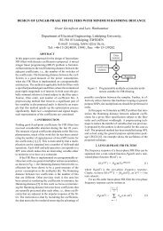
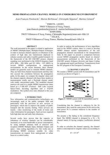
where the superscript . H denotes the Hermitian transpose,S and D are respectively Nr Nr and Nt Nt unitarymatrix and V is a Nr Nt diagonal matrix such as (2).V = diag( 1 , 2 , …, N ) (2)with 1 2 … N 0, i being the i-th singular valueof H and N = min(Nr, Nt)The MIMO channel capacity is obtained with relation(3).C Nk12. klog 2 (1)Nt(3)with the average signal-to-noise ratio at each receiverbranch.Considering that the square of the singular values arealso the eigen values of H.H H , the MIMO channelcapacity can finally be expressed by the equation (4) [1]. C log 2 det(I Nr H . H NtH(4)3. MEASUREMENTSChannel matrices H were measured by the TELICELaboratory (France) in a subway tunnel in Paris [3]. Thiswas done in the framework of the ESCORT projectusing a transmission in the GSM-R frequency band. TheMIMO system is composed of 4 antennas in the train and4 fixed antennas put on a platform. For each position ofthe train, a measurement of the complex impulseresponse between each transmitter and receiver is carriedout. Considering the small delay spread (about 50 ns)obtain in tunnel compared to a typical GSM symbolduration (3.7 s), the impulse responses may be reducedto a complex coefficient. Thus, we obtained for eachposition of the train a 4 4 matrix. The longitudinalattenuation is removed from channel measurements, sothat the matrices H were in accordance with equation (5).E[|h ij | 2 ] = 1 (5)The measured channel matrices allow to compute thecorrelation matrix and the covariance matrix definedbelow.4. MIMO CHANNEL MODELSIn the following we compare three channel models to aRayleigh channel and to measurements results.4.1 Model 1 based on covarianceThis model [4] relies on the computation of thecovariance matrix at the transmitter R TX (Nt Nt) and atthe receiver R RX (Nr Nr).At the transmitter, the covariance coefficient between thei-th and the j-th antenna is expressed in (6) by assumingthat it is independent of the reception antennasNrTX 1ij cov( hki,hkj)Nrk1r (6)At the receiver, the covariance coefficient between the i-th and the j-th antenna is expressed in (7) by assumingthat it is independent of the transmission antennasNtRX 1ij cov( hik,h jk )Ntk 1r (7)We note cov(a, b) the covariance coefficient between aand b such as (8)cov(a, b) = E[a.b * ] – E[a].E[b * ] (8)Then, the channel model matrix is built from (9) asfollowsH model = (R RX ) 1/2 . A.[(R TX ) 1/2 ] T (9)where A is a stochastic Nr Nt matrix with a zero-meancomplex Gaussian distribution with unit variance andmatrix R 1/2 is defined such as R 1/2 .(R 1/2 ) H = R.4.2 Model 2 based on complex correlationAs previously, we define the correlation matrix at thetransmitter TX (Nt Nt) and at the receiver RX(Nr Nr) such as (10) and (11)NrTX 1ij cor( hki,hkj)Nrk1 (10)NtRX 1ij cor( hik,h jk )Ntk 1 (11)We note cor(a, b) the correlation coefficient between aand b defined in (12):cor( a,b )( E[ a2E[ a.b*] E[ a ]] E[ a ].E[ b2).( E[ b2*]] E[ b]2)(12)By assuming that the correlation matrix at the transmitteris independent of the receiver antennas and that thecorrelation matrix at the receiver is independent of thetransmitter antennas [5], the channel correlation matrix (Nt.Nr Nt.Nr) can be expressed as (13)

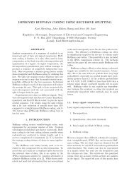
Type of H H complx H power H cov H Raylchannelmatrixcorr corr 1 4.12 3.77 3.86 4.08 3.10 2 0.32 0.29 0.48 0.30 2.07 3 0.12 0.06 0.14 0.06 1.22 4 0.04 0.01 0.04 0.01 0.44Table 2 : Average of the singular values forConfiguration 2The corresponding channel capacities mean values for anaverage signal-to-noise ratio of 10 dB are given inTable 3 and 4. The models based on complex correlationand covariance show good agreement with themeasurements for the two antenna configurations. Themodel based on power correlation does not fit correctlythe measurements in the first configuration where thecorrelation is lower. As previously, the two best modelsin the case of configuration 1, are those based on thecomplex correlation and on the covariance.4.4.3. Channel capacityIn Figure 7 and Figure 8, we present the cumulativedensity functions of the capacity.Type of H H complx H power H cov H Raylchannelmatrixcorr corrC 8.44 8.76 9.26 7.97 10.94Table 3 : Average channel capacities for = 10 dB inbits/s/Hz for Configuration 1CDF10.90.80.70.60.50.4HH complex corrH power corrH covH RaylType of H H complx H power H cov H Raylchannelmatrixcorr corrC 5.76 5.31 5.87 5.52 10.96Table 4 : Average channel capacities for = 10 dB inbits/s/Hz for Configuration 20.30.20.104 6 8 10 12 14 16Channel capacity (bit/s/Hz)Figure 7 : CDF of the capacity for Configuration 1 with = 10 dB4.4.4. Symbol Error RateWe simulated a 4-QAM transmission using the V-BLAST (Vertical – Bell Labs Layered Space-Time)decoding algorithm. As previously, the channel isaccounted for by using our 3 models, measured channelmatrices or the uncorrelated MIMO Rayleigh channel.Symbol error rate obtained for Configuration 1 and 2 arerespectively presented Figure 9 and Figure 10.10.90.8HH complex corrH power corrH covH Rayl10 0 SNR (dB)0.7CDF0.60.510 -10.40.30.2Symbol Error Rate10 -20.110 -300 2 4 6 8 10 12 14 16Channel capacity (bit/s/Hz)Figure 8 : CDF of the capacity for Configuration 2 with = 10 dB10 -4HH complex corrH power corrH covH Rayl0 5 10 15 20 25 30 35 40Figure 9 : Symbol error rate versus Signal to NoiseRatio (SNR) for Configuration 1

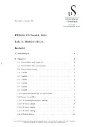
why these two models sometimes lead to differentresults.10 0 SNR (dB)Symbol Error Rate10 -110 -210 -310 -4HH complex corrH power corrH covH Rayl0 5 10 15 20 25 30 35 40Figure 10 : Symbol error rate versus Signal to NoiseRatio (SNR) for Configuration 2APPENDIXIn order to demonstrate that the model based on complexcorrelation and the model based on covariance areequivalent, we need that :iforifR1 / 2 R1 / 2rxR R rx R tx1 / 2 1 / 2rx rx tx R 1 / 2tx1 / 2txWe can note that symbol error rate are quite high, this isdue to the important correlation between the paths. Forthe first configuration, all the models fit well themeasurements, except the model based on covariance.Surprisingly, for the second configuration, only themodel based on power shows good agreement withmeasurements.CONCLUSION AND PERSPECTIVESIn this paper, we have compared three MIMO channelmodels to a simulation using real channel matricesmeasured in underground environment in the GSM-Rfrequency band. Regarding the singular values and thechannel capacity, the best models among the three arethose based on covariance and complex correlation.When the symbol error rate is considered, the modelbased on power correlation provides better agreementwith measurements in the case of a 4-QAM modulationand a V-BLAST decoding algorithm. The three modelsare very close and it is difficult to choice the morerealistic one.This study was performed only on two measurementconfigurations with relatively high correlation betweenpaths. Other measurements under low correlationcondition are necessary to state on model’s efficiency.Moreover, the number of channel matrices H, effectivelymeasured, is quite small (75 measured channel matricesfor Configuration 1 and 53 for Configuration 2). Thedistance between two measurements is about sixwavelengths, which is too long to analyse accurately themultipath effects. For these reasons, we have plan newmeasurements in the 5 GHz HIPERLAN frequencyband.Furthermore, models based on complex correlation andcovariance matrices are mathematically similar to eachother. (See appendix). We must investigate the reasonREFERENCES[1] G.J. Foschini, M.J. Gans, "On Limits of WirelessCommunications in a Fading Environment When UsingMultiple Antennas", Wireless Personal Communications,Vol. 6, n°3, March 1998, pp. 311-335[2] G.H. Golub, C.F. Van Loan, “Matrix Computations”,Third Edition, The John Hopskins University Press,1996[3] Martine Liénard, Jacques Baudet, Daniel Degardin,Pierre Degauque, "Capacity of Multi-Antenna ArraySystems in Tunnel Environment", IEEE Int. Conf. onVehic. Tech., Birmingham, Alabama, 4 - 9 May 2002[4] K. Yu, M. Bengtsson, B. Ottersten, D. McNamara, P.Karlsson, M. Beach, “Second Order Statistics of NLOSIndoor MIMO Channels Based on 5.2 GHzMeasurements”, Proceedings Global CommunicationsConference 01’, San Antonio, Texas, USA, November,2001[5] K.I. Pedersen, J. B. Andersen, J.P. Kermoal, P.Mogensen, “A Stochastic Multiple-Input-Multiple-Output Radio Channel Model for Evaluation of Space-Time Coding Algorithms”, Vehicular TechnologyConference Fall 2000[6] J.P. Kermoal, L. Schumacher, P.E. Mogensen, K.I.Pedersen, “Experimental Investigation of CorrelationProperties of MIMO Radio Channels for Indoor PicocellScenarios”, IEEE Vehicular Technology ConferenceVTC 2000 Fall, Boston, USA, 2000[7] S.R. Saunders, “Antennas and Propagation forWireless Communication Systems”, Wiley, 2001,pp 371-372