- Page 1 and 2:
command the brilliance of a thousan
- Page 3 and 4:
ii•Waterloo Maple Inc.57 Erb Stre
- Page 6 and 7:
Contents • v3.6 Interfaces and Im
- Page 8 and 9:
Contents • viiPlotting Gears . .
- Page 10 and 11:
Contents • ixForeign Data . . . .
- Page 12 and 13:
1 Introduction1.1 Purpose of This B
- Page 14 and 15:
2 Procedures, Variables,and Extendi
- Page 16 and 17:
2.1 Nested Procedures • 5procedur
- Page 18 and 19:
2.1 Nested Procedures • 7> A[j] :
- Page 20 and 21:
2.1 Nested Procedures • 9> quicks
- Page 22 and 23:
2.1 Nested Procedures • 11> U :=
- Page 24 and 25:
2.2 Procedures That Return Procedur
- Page 26 and 27:
2.2 Procedures That Return Procedur
- Page 28 and 29:
2.3 Local Variables and Invoking Pr
- Page 30 and 31:
assign(another_a = a);> eqn;2.3 Loc
- Page 32 and 33:
[ seq( s[j][c[j]], j=1..2 ) ];2.3 L
- Page 34 and 35:
2.3 Local Variables and Invoking Pr
- Page 36 and 37:
2.4 Interactive Input • 25Improve
- Page 38 and 39:
2.4 Interactive Input • 27> reads
- Page 40 and 41:
2.5 Extending Maple • 29The parse
- Page 42 and 43:
2.5 Extending Maple • 31> ‘type
- Page 44 and 45:
2.5 Extending Maple • 33The follo
- Page 46 and 47:
2.5 Extending Maple • 3556 IIn th
- Page 48 and 49:
2.5 Extending Maple • 37Extending
- Page 50 and 51:
2.5 Extending Maple • 39The useri
- Page 52 and 53:
3 Programming withModulesProcedures
- Page 54 and 55:
• 43> gentemp := proc()> count :=
- Page 56 and 57:
3.1 Syntax and Semantics3.1 Syntax
- Page 58 and 59:
3.1 Syntax and Semantics • 47name
- Page 60 and 61:
3.1 Syntax and Semantics • 49> He
- Page 62 and 63:
3.1 Syntax and Semantics • 51mode
- Page 64 and 65:
3.1 Syntax and Semantics • 53The
- Page 66 and 67:
3.1 Syntax and Semantics • 55true
- Page 68 and 69:
3.1 Syntax and Semantics • 57modu
- Page 70 and 71:
3.1 Syntax and Semantics • 59> m
- Page 72 and 73:
This is achieved by the double assi
- Page 74 and 75:
3.1 Syntax and Semantics • 63This
- Page 76 and 77:
3.1 Syntax and Semantics • 65With
- Page 78 and 79:
3.1 Syntax and Semantics • 67> wh
- Page 80 and 81:
SpecFuncs := module()> export F; #
- Page 82 and 83:
3.2 Records • 71b> evalb( % = b )
- Page 84 and 85:
3.3 Packages • 73Packages in the
- Page 86 and 87:
3.3 Packages • 751 −1 + 1 21k x
- Page 88 and 89:
3.3 Packages • 77> "new types ‘
- Page 90 and 91:
3.3 Packages • 79definition. This
- Page 92 and 93:
3.3 Packages • 81true> member( 10
- Page 94 and 95:
3.3 Packages • 83The display show
- Page 96 and 97:
3.3 Packages • 85> end module:How
- Page 98 and 99:
3.3 Packages • 87From the output
- Page 100 and 101:
3.3 Packages • 89The final output
- Page 102 and 103:
3.3 Packages • 91shape-specific f
- Page 104 and 105:
3.3 Packages • 93The area Procedu
- Page 106 and 107:
"but got %1", shape> end if;>> # Ex
- Page 108 and 109:
3.4 The use Statement • 97> circl
- Page 110 and 111:
3.4 The use Statement • 99use sta
- Page 112 and 113:
3.4 The use Statement • 101C++),
- Page 114 and 115:
3.5 Modeling Objects3.5 Modeling Ob
- Page 116 and 117:
3.5 Modeling Objects • 10514 πFo
- Page 118 and 119:
3.5 Modeling Objects • 107> nitem
- Page 120 and 121:
3.5 Modeling Objects • 109> for i
- Page 122 and 123:
3.5 Modeling Objects • 111> lengt
- Page 124 and 125:
3.6 Interfaces and Implementations
- Page 126 and 127:
3.6 Interfaces and Implementations
- Page 128 and 129:
3.6 Interfaces and Implementations
- Page 130 and 131:
3.6 Interfaces and Implementations
- Page 132 and 133:
3.6 Interfaces and Implementations
- Page 134 and 135:
3.6 Interfaces and Implementations
- Page 136 and 137:
3.6 Interfaces and Implementations
- Page 138 and 139:
3.6 Interfaces and Implementations
- Page 140 and 141:
3.6 Interfaces and Implementations
- Page 142 and 143:
3.6 Interfaces and Implementations
- Page 144 and 145:
(−2790 T 6 − 77814+ 1943715124T
- Page 146 and 147:
3.6 Interfaces and Implementations
- Page 148 and 149:
3.6 Interfaces and Implementations
- Page 150 and 151:
3.6 Interfaces and Implementations
- Page 152 and 153:
3.6 Interfaces and Implementations
- Page 154 and 155:
3.6 Interfaces and Implementations
- Page 156 and 157:
3.6 Interfaces and Implementations
- Page 158 and 159:
3.6 Interfaces and Implementations
- Page 160 and 161:
3.6 Interfaces and Implementations
- Page 162 and 163:
3.6 Interfaces and Implementations
- Page 164 and 165:
3.6 Interfaces and Implementations
- Page 166 and 167:
4 Input and OutputAlthough Maple is
- Page 168 and 169:
4.1 A Tutorial Example • 157Openi
- Page 170 and 171:
4.1 A Tutorial Example • 159xy :=
- Page 172 and 173:
Buffered Files:4.2 File Types and M
- Page 174 and 175:
4.3 File Descriptors versus File Na
- Page 176 and 177:
f := fopen("testFile.txt",WRITE):>
- Page 178 and 179:
4.5 Input Commands • 167iostatus(
- Page 180 and 181:
4.5 Input Commands • 169otherwise
- Page 182 and 183:
4.5 Input Commands • 171y The nex
- Page 184 and 185:
4.5 Input Commands • 173various c
- Page 186 and 187:
4.5 Input Commands • 175Example T
- Page 188 and 189:
4.6 Output Commands • 177One-Dime
- Page 190 and 191:
4.6 Output Commands • 179the appr
- Page 192 and 193:
4.6 Output Commands • 181Writing
- Page 194 and 195:
4.6 Output Commands • 183z format
- Page 196 and 197:
4.6 Output Commands • 185• If n
- Page 198 and 199:
4.6 Output Commands • 187> writed
- Page 200 and 201:
4.7 Conversion Commands • 189Conv
- Page 202 and 203:
4.8 Notes to C Programmers • 191(
- Page 204 and 205:
5 Numerical Programmingin MapleFloa
- Page 206 and 207: 5.1 The Basics of evalf • 1953.14
- Page 208 and 209: 5.2 Hardware Floating-Point Numbers
- Page 210 and 211: 5.2 Hardware Floating-Point Numbers
- Page 212 and 213: iterate(f, df, x0, N);> end proc:Us
- Page 214 and 215: 5.2 Hardware Floating-Point Numbers
- Page 216 and 217: 5.3 Floating-Point Models in Maple
- Page 218 and 219: 5.3 Floating-Point Models in Maple
- Page 220 and 221: 5.4 Extending the evalf Command •
- Page 222 and 223: 5.4 Extending the evalf Command •
- Page 224 and 225: 5.5 Using the Matlab Package • 21
- Page 226 and 227: 6 Programming with MapleGraphicsMap
- Page 228 and 229: 6.1 Basic Plot Functions • 217If
- Page 230 and 231: 6.2 Programming with Plotting Libra
- Page 232 and 233: 6.2 Programming with Plotting Libra
- Page 234 and 235: 6.2 Programming with Plotting Libra
- Page 236 and 237: 6.3 Maple Plotting Data Structures
- Page 238 and 239: 6.3 Maple Plotting Data Structures
- Page 240 and 241: 6.3 Maple Plotting Data Structures
- Page 242 and 243: PLOT( CURVES( points ) );6.3 Maple
- Page 244 and 245: 6.3 Maple Plotting Data Structures
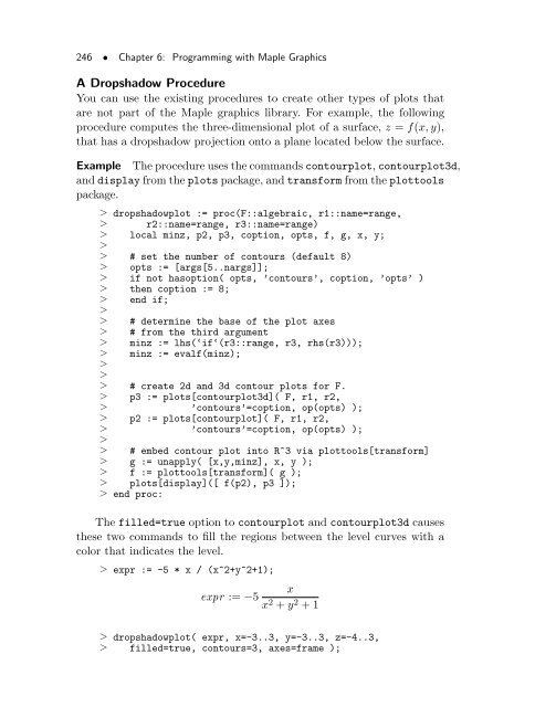
- Page 246 and 247: 6.4 Programming with Plot Data Stru
- Page 248 and 249: 6.4 Programming with Plot Data Stru
- Page 250 and 251: 6.4 Programming with Plot Data Stru
- Page 252 and 253: 6.4 Programming with Plot Data Stru
- Page 254 and 255: 6.5 Programming with the plottools
- Page 258 and 259: 6.5 Programming with the plottools
- Page 260 and 261: 6.5 Programming with the plottools
- Page 262 and 263: 6.5 Programming with the plottools
- Page 264 and 265: 6.5 Programming with the plottools
- Page 266 and 267: 6.5 Programming with the plottools
- Page 268 and 269: 6.6 Vector Field Plots • 257Examp
- Page 270 and 271: 6.6 Vector Field Plots • 259> end
- Page 272 and 273: 6.6 Vector Field Plots • 261input
- Page 274 and 275: 6.6 Vector Field Plots • 263> mak
- Page 276 and 277: 6.6 Vector Field Plots • 265> vec
- Page 278 and 279: 6.7 Generating Grids of Points •
- Page 280 and 281: A := array(1..2, 1..2):> evalgrid(
- Page 282 and 283: 6.8 Animation • 271The gridpoints
- Page 284 and 285: 6.8 Animation • 2731.00.500. 0. 2
- Page 286 and 287: 6.8 Animation • 275> partsum := p
- Page 288 and 289: 6.8 Animation • 277Demonstrating
- Page 290 and 291: plot3d( p, -3..3, -3..3, color=q );
- Page 292 and 293: 6.9 Programming with Color • 2811
- Page 294 and 295: 6.9 Programming with Color • 283>
- Page 296 and 297: 6.9 Programming with Color • 2851
- Page 298 and 299: chessplot3d( sin(x)*sin(y), x=-Pi..
- Page 300 and 301: 7 Advanced ConnectivityIn This Chap
- Page 302 and 303: 7.1 Code Generation • 291Many opt
- Page 304 and 305: 7.2 Using Compiled Code in Maple
- Page 306 and 307:
7.2 Using Compiled Code in Maple
- Page 308 and 309:
7.2 Using Compiled Code in Maple
- Page 310 and 311:
7.2 Using Compiled Code in Maple
- Page 312 and 313:
7.2 Using Compiled Code in Maple
- Page 314 and 315:
7.2 Using Compiled Code in Maple
- Page 316 and 317:
7.2 Using Compiled Code in Maple
- Page 318 and 319:
7.2 Using Compiled Code in Maple
- Page 320 and 321:
7.2 Using Compiled Code in Maple
- Page 322 and 323:
7.2 Using Compiled Code in Maple
- Page 324 and 325:
char * concat( char* a, char *b ){c
- Page 326 and 327:
7.2 Using Compiled Code in Maple
- Page 328 and 329:
7.2 Using Compiled Code in Maple
- Page 330 and 331:
myAdd = to_maple_integer( kv, r )EN
- Page 332 and 333:
7.2 Using Compiled Code in Maple
- Page 334 and 335:
to_maple_char( kv, c )to_maple_comp
- Page 336 and 337:
7.2 Using Compiled Code in Maple
- Page 338 and 339:
7.2 Using Compiled Code in Maple
- Page 340 and 341:
7.2 Using Compiled Code in Maple
- Page 342 and 343:
7.2 Using Compiled Code in Maple
- Page 344 and 345:
7.2 Using Compiled Code in Maple
- Page 346 and 347:
7.2 Using Compiled Code in Maple
- Page 348 and 349:
7.3 System Integrity • 337by anot
- Page 350 and 351:
Table 7.3 Wrapper Compound TypesMap
- Page 352 and 353:
AInternal Representationand Manipul
- Page 354 and 355:
A.1 Internal Organization • 343wi
- Page 356 and 357:
A.2 Internal Representations of Dat
- Page 358 and 359:
Type Specification or TestA.2 Inter
- Page 360 and 361:
A.2 Internal Representations of Dat
- Page 362 and 363:
Length: 3 or moreA.2 Internal Repre
- Page 364 and 365:
A.2 Internal Representations of Dat
- Page 366 and 367:
A.2 Internal Representations of Dat
- Page 368 and 369:
A.2 Internal Representations of Dat
- Page 370 and 371:
A.2 Internal Representations of Dat
- Page 372 and 373:
A.2 Internal Representations of Dat
- Page 374 and 375:
A.2 Internal Representations of Dat
- Page 376 and 377:
A.2 Internal Representations of Dat
- Page 378 and 379:
A.3 The Use of Hashing in Maple •
- Page 380 and 381:
A.3 The Use of Hashing in Maple •
- Page 382 and 383:
A.3 The Use of Hashing in Maple •
- Page 384 and 385:
Index%, 174&, 31accuracy, 193, 195,
- Page 386 and 387:
Index • 375SAVE, 362SERIES, 363SE
- Page 388 and 389:
Index • 377defining numeric, 210n
- Page 390 and 391:
Index • 379name, 357name table, 3
- Page 392 and 393:
Index • 381statements, 174strings
- Page 394:
Waterloo Maple Inc.57 Erb Street We