Amplifier Frequency Response - Ken Kuhn's

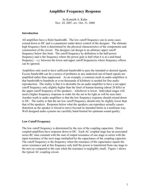
Amplifier Frequency Responseby Kenneth A. KuhnNov. 24, 2007, rev. Oct. 31, 2008IntroductionAll amplifiers have a finite bandwidth. The low cutoff frequency can in some casesextend down to DC and is a parameter under direct control of the designer. The ultimatehigh frequency limit is determined by the physical characteristics of the components andconstruction of the circuit. The designer can design to an arbitrary upper cutofffrequency below this limit. The cutoff frequency by definition is the half-powerfrequency and is the frequency where the power gain is half what it is at a mid-bandfrequency–i.e. between the lower and upper cutoff frequencies where frequency effectscan be ignored.Amplifiers only need to have sufficient bandwidth to pass the intended or desired signals.Excess bandwidth can be a source of problems as any undesired out-of-band signals areamplified rather than suppressed. As an example, a common myth in audio amplifiers isthat bandwidth to hundreds or even thousands of kilohertz is needed for fine audioreproduction. The reality is that it is desirable for an audio amplifier to have a net uppercutoff frequency only slightly higher than the limit of human hearing (about 20 kHz) orthe upper cutoff frequency of the speakers–whichever is lower. Individual stages willneed a higher frequency response in order for the net to be right as will be seen later.Another myth in audio amplifiers is that the low frequency response should extend downto DC. The reality is that the net low cutoff frequency should only be slightly lower thanthat of the speakers. Response below what the speakers can reproduce actually causesdistortion as the speaker is forced to move beyond its intended limits in a nonlinear way.Well designed audio systems are carefully band-limited for optimum sound quality.Low Cutoff FrequencyThe low cutoff frequency is determined by the size of the coupling capacitors. Directcoupled amplifiers have response down to DC. Each AC coupled stage has an associatedseries RC time constant with the sum of output resistance of one stage in series with theinput resistance of the next stage multiplied by the capacitance of the coupling capacitor.The cutoff frequency is the frequency when the reactance of the capacitance equals theseries resistance and at this frequency only half the power is transferred from one stage tothe next as compared to the case when the reactance is negligibly small. Figure 1 showsthe typical AC coupling circuit.1

Amplifier Frequency ResponseThe low cutoff frequency isFigure 1: AC coupling, series circuitFcl = 1 / (2 * π* Rseries * Cseries) Eq. 1An amplifier typically has several AC couplings from input to output. The question ishow to compute the net low cutoff frequency of a chain of AC coupled stages.Computing the exact cutoff frequency is impractical for hand calculations–the highorder math is best done via a computer. For many problems an exact answer is notnecessary and a reasonable approximation is fine. A popular approximation is as followsFcl_net ~= sqrt(Fcl1 2 + Fcl2 2 + … Fcln 2 ) Eq. 2It should be obvious from Eq. 2 that Fcl_net will always be higher than the highestindividual cutoff frequency. Another observation is that the higher cutoff frequenciesstrongly dominate the result. The accuracy of Eq. 2 is reasonable for most cases and istypically better than twenty percent. The accuracy is worst if most individual cutofffrequencies are nearly the same–the error can be several tens of percent.The design process is determining the proper size capacitors to use for each coupling inorder to achieve the desired net low cutoff frequency. In thinking about how one shoulddistribute the time constants for each coupling the thought should occur to make all timeconstants the same–thus the low cutoff frequency is identical for all couplings. Thisconcept greatly simplifies what otherwise would be a huge guessing game. From earlierdiscussion it should be noted that the individual cutoff frequency for each coupling mustbe lower in order to net a target net low cutoff frequency. The question for the designeris how much lower? Simplistically, one might think that the cutoff frequency should bethe target cutoff frequency divided by the number of AC coupling but this turns out to beoverkill. Each stage only has to reduce the power transfer by one nth of half. Thisproblem is readily solved via a computer that raises the first order transfer function to thenth power and then solves for the resultant cutoff frequency using numerical methods.2

Amplifier Frequency ResponseSince that calculation is always the same a simple table of results can be generated asshown below.Number of Stages Factor of individual cutoff frequency to net cutoff frequency1 1.0002 0.6443 0.5104 0.4355 0.3866 0.3507 0.3238 0.3019 0.28310 0.268Table 1Table adapted from Analysis and Design of Integrated Electronic Circuits, second edition, by Paul M.Chirlian, Harper and Row, 1987, page 589From Table 1 if we are designing an amplifier that has three AC couplings and we desirea net low cutoff frequency of 100 Hz, then each coupling should have a cutoff frequencyof 51 Hz. It is not necessary to hit this exactly and the common tactic is to calculate therequire capacitance for each stage and round up to the next standard or convenientcapacitor size. This will result in a net cutoff frequency of slightly less than 100 Hz butthe interpretation of the design specification should be“not higher than 100 Hz.”A littlelower cutoff frequency is fine.AC couplings include stage to stage coupling plus emitter bypass capacitors in commonemitteramplifiers. The resistance for the time constant calculation is that of R E 1 (whichmight be zero) plus the dynamic emitter resistance, re. The emitter bias resistor, R E , isalso involved but that effect is usually small and is more than compensated by therounding up to the next larger capacitor size discussed earlier. Figure 2 shows the typicalcircuit.3

Amplifier Frequency ResponseFigure 2: AC coupling, series circuit in emitterIt should be noted then that a simple single stage common-emitter amplifier has a total ofthree AC couplings–the input, the emitter bypass, and the output.High Cutoff FrequencyThe ultimate high cutoff frequency of an amplifier is determined by the physicalcapacitances associated with every component and of the physical wiring. Transistorshave internal capacitances that shunt signal paths thus reducing the gain. The high cutofffrequency is related to a shunt time constant formed by resistances and capacitancesassociated with a node. We are stuck with the physical capacitances (typically in thesingle and low double digit picofarrad range) so the primary option for very highfrequency response is low value resistances. Another option is much smaller componentswhich in turn have lower capacitances. In some cases, small inductances can built intothe circuit to counteract the capacitances. The ultimate in extremely high frequencyresponse is achieved by building the amplifier as a matched transmission line.Figure 3 shows the typical circuit that becomes significant at high frequencies. Note thatCin could be the sum of several different capacitances. These capacitances are from thephysics of the components and construction and are not arbitrary. Only sometimes arethese capacitances intentional components4

Amplifier Frequency ResponseFigure 3: Shunt capacitance at high frequencyThe high cutoff frequency of each node of an amplifier is inversely proportional to thenet shunt resistance and net shunt capacitance and is given byFch = 1 / (2 *π * Rshunt * Cshunt) Eq. 3This equation is identical to Equation 1 except that the resistances and capacitances are inshunt rather than in series. A given amplifier will have several high cutoff frequencies.The net high cutoff frequency is a challenge to calculate manually but a popularapproximation is1Fch_net ~= ----------------------------------------------- Eq. 4sqrt(1/Fcl1 2 + 1/Fcl2 2 + … Fcln 2 )The Fch_net will always be lower than the lowest individual cutoff frequency. The lowercutoff frequencies will also dominate the result. Like Equation 2, the approximation isgenerally good to around twenty percent unless most cutoff frequencies are similar–thenthe accuracy degrades to several tens of percent.It is often the case that we do not want wide bandwidth in an amplifier and the designerwill add capacitance to lower the bandwidth to the desired amount.The primary discussion here is the internal capacitances of a transistor and how thoseaffect the high frequency response. The transistor internal capacitances are proportionalto the physical area of the junctions and inversely proportional to the width of thedepletion region, i.e. the classic physics of a capacitor. For a simple transistor modelthere are only two capacitances we will consider–C BC which is between the base andcollector junctions and C BE which is between the base and emitter junction as shown inFigure 4. This means that the capacitance is a function of bias conditions. A forwardbiased junction has relatively high capacitance (tens to over one hundred picofarradsdepending on forward current) because the width of the depletion region is narrow. A5

Amplifier Frequency Responsereversed biased junction has relatively low capacitance (typically less than tenpicofarrads and even less than one picofarrad in some cases) because the width of thedepletion region is wide. These capacitance effects are shown in Figure 5. The fact thatjunction capacitance is inversely related to reverse voltage is a useful characteristic that isused for electronic tuning of radio frequency networks. For high frequency amplifiers wegenerally want to operate the transistor with as high a reverse bias on the base-collectorjunction as practical to minimize that capacitance. This means that V CB min should begreater than 4 volts.Figure 4: Transistor capacitancesFigure 5: PN junction capacitance curveThe Miller effectIn the early days of vacuum tube amplifiers it was observed that high gain amplifiersbuilt with common-cathode (analogous to common-emitter or common-source)architectures had much lower than expected high frequency response. An engineerwhose name was Miller discovered the reason why. The small capacitance that exists6

Amplifier Frequency Responsefrom the output of the amplifier to the input was magnified by the amplifier gain andappeared as a large shunt capacitance across the input of the amplifier. In those days thecapacitance was between the plate and grid which is analogous today to capacitancebetween the collector and base (i.e. C F = C BC ). The Miller effect occurs only in invertingamplifiers–it is the inverting gain that magnifies the feedback capacitance. Note thatone side of the capacitor is connected to the input signal and the other side is connectedto the larger in magnitude and phase inverted output signal. This causes the reactivecurrent through the capacitor to be (|Gain| + 1) higher than what would exist if thefeedback capacitance were only across the input–thus the capacitor appears larger by thefactor of (|Gain| + 1). This causes a significant low frequency pole to exist and limitsamplifier bandwidth. Note that the absolute value of gain is used to eliminate sign errorssince the actual sign of the gain is minus.Figure 6: Miller effect7

Amplifier Frequency ResponseAn example problemThe transistor circuit in Figure 7 will be analyzed for low and high cutoff frequencies.The summary results from bias analysis and AC analysis are shown. We use the resultsfrom AC analysis to do frequency response analysis. Note that a significant value forC BC has been inserted to arbitrarily lower the high frequency bandwidth.Figure 7: Example circuitV CC = 12V, R S = 1K, R B 1 = 150K, R B 2 = 22K, RE = 1.5K, R C = 10K, R L = 10K,C B = 1 uF, CE = 100 uF, CC = 0.1 uF, C BC = 1 nF, CL = 1 nF,Not shown are: C BE = 30 pF, Cin_stray = 25 pF, Co stray = 20 pFSummary bias and AC analysis using B = 150 and V BE = 0.65V BB = 1.53 VR B = 19.2 KI E = 541 uAI C = 537 uAV C = 6.6 Vr e = 48 ohmsrbt = 7.25KR in = 5.26 KR o = 10KAv = 207Avl = 1038

Amplifier Frequency ResponseLow Frequency AnalysisFcl1 = 1 / (6.28 * (1K + 5.26K) * 1 uF) = 25.4 HzFcl2 = 1 / (6.28 * (48 + 0) * 100 uF) = 33.2 Hz (note: RE1 = 0)Fcl3 = 1/(6.28 * (10K + 10K) * 0.1 uF) = 79.6 HzFcl_net ~= sqrt(25.4^2 + 33.2^2 + 79.6^2) = 89.9 HzHigh Frequency AnalysisCmiller = 1.0 nF * (103 + 1) = 104 nF (note that we use Avl and C BC )Cin_total = 104 nF + 30 pF + 20 pF = 104.05 nF (note how Cmiller dominates)Rin_shunt = 1K || 5.26K = 840 ohmsFch1 = 1 / (6.28 * 840 * 104.05 nF) = 1.81 kHzCout_shunt = 20 pF + 1 nF = 1.02 nFRo_shunt = 10K || 10 K = 5KFch2 = 1 / (6.28 * 5K * 1.02 nF) = 31.2 kHzFch_net ~= 1 / (sqrt(1/1.81 kHz^2 + 1/31.2 kHz^2) = 1.81 kHz9