Lyapunov-Based Control Scheme for Single-Phase Grid ... - ITM

522 IEEE TRANSACTIONS ON CONTROL SYSTEMS TECHNOLOGY, VOL. 20, NO. 2, MARCH 2012rameters of this model can be defined as, and , where andare the number of PV cells connected in series and parallel,respectively.B. Power Conditioning SystemThe schematic diagram of the full-bridge central inverter configurationis shown in Fig. 1. Here and are the averagevalues of the input capacitor voltage and the output inductor current,respectively. The utility grid voltage is assumed to besinusoidal with a constant amplitude and a constant frequency, i.e., . The full-bridge inverter consists of fourswitches controlled by the signals and which take values inthe discrete set (i.e., OFF or ON, respectively). The switchcontrol signals are generated via a PWM scheme with a dutyratio functiongenerated by the controller. Thismeans that if the switching frequency is sufficiently high, thedynamical behavior of the GPV system can be approximated bythe following set of differential equations:(4)(5)The latter equations will be used to design a controller for thesystem, where we assume that the only unknown parameter is. The controller should be able to deal with this parameteruncertainty.III. CONTROLLER DESIGNA. Control ObjectivesThe GPV inverter of Fig. 1 should be able to transfer efficientlythe maximum amount of PV energy to the utility grid. Inorder to accomplish that the following is required.C1) to deliver a sinusoidal current in phase with the utilityvoltage of the power grid;C2) to regulate the input capacitor voltage to a value thatassures maximum power extraction from the PV array.With respect to C2, it should be mentioned that it is assumedthat the reference capacitor voltage value is given by an externalmaximum power point tracking (MPPT) algorithm. MPPT algorithmsoperate based on the changes of temperature and solarirradiance and therefore change very slowly compared to the dynamicsof the power inverter. For instance, slow varying MPPTs(variation time 20 ms), such as an extremum-seeking [30] orothers based on heuristic approaches [31] may be added to thisscheme without affecting the dynamic behavior of the analyzedclosed-loop system.Based on (4) and the notation presented in Section II, objectivesC1 and C2 translate into, whereand is the value of such that is maximum. Thepower generated by the PV panels equals .Ideally, should be a constant in order to assure that thePV array operating point remains always in its maximum power(6)point. However, due to the intrinsic nature of the inverter structureused it is not possible to have a sinusoidal output currentand a constant input voltage. This impossibility can be seen assumingthatand obtaining the energy-balanceequation of the system from (4)Notice that this expression is independent from the controlsignal . Substituting (6) into (7) yields(8)where we recall that .From (8) it is clear that has to be time-varying. Nevertheless,a time-varying is an undesired effect because it willmove the PV array operating point from its maximum powerpoint. A practical solution for this problem, widely used in thedesign of Central PV inverters, is to make sufficiently largeto reduce the oscillations towards the PV array maximum powerpoint. Indeed, as is shown next, obtained from (8) is a periodicsignal with an offset value , such that whenis sufficiently large 1 .For analysis convenience instead of consider the energystored in the capacitor, i.e.,and substitute itin (8) obtainingInstead of obtaining the exact analytical solution of (9) wewill solve its linearized version. Given that we will have a sufficientlylarge the linearization of (9) is a very good approximationas it will be shown. 2 Linearizing the nonlinear functionaround the dc value of (denoted as ) yieldswhereHence, (9) reduces to(7)(9)(10)(11)(12)1 Notice that having a C sufficiently large is a requirement for this type ofpower inverters, given that smaller values of C may reduce considerable theamount of energy extracted from the PV array.2 Take into account that this linearization process is only done in order to estimatethe waveform of the desired steady-state value x and to verify that it isperiodic. In the remainder of the article we will be working with the nonlineardynamics of the system.

524 IEEE TRANSACTIONS ON CONTROL SYSTEMS TECHNOLOGY, VOL. 20, NO. 2, MARCH 2012vanishes. The error dynamics are obtained by substituting (17)in (19), i.e.,(20)Notice that in our case we do not only have to synthesize thecontrol that renders the error dynamics (20) stable, but weshould derive an additional mechanism to estimate parameter, i.e., to make . In order to proof the validity of our controlscheme the final stability analysis should take into accountthe designed signal and the dynamics associated to the estimationof .In order to estimate , the following adaptive law, taken from[19], is used:ifotherwise(21)where is the adaptive gain and is a projectionoperator that ensures , with an arbitrary smallconstant.The stability of the error dynamics (20) can be proved bymeans of the following Lyapunov function(22)for which the time derivative along the system trajectories of(20) yields(23)The closed-loop system will be globally asymptotically stable ifthe aforementioned expression is negative definite, i.e., iffor all values of different from zero. Defining as(24)where is a control parameter, the first term of (23) remainsalways non-positive, i.e.,(25)On the other hand, considering “locally constant”, yields, and according to (21), , and thus, thederivative of the Lyapunov function (25) can be written as(26)Notice that the productis always positive giventhat function is strictly increasing, i.e., the functionis positive whenand negativewhen . Thus, the closed-loop system (19), using thecontrol signal (18), (24) and the adaptive control law (21), isglobally asymptotically stable.IV. PRACTICAL CONSIDERATIONSIn this section, some practical considerations regarding thepreviously derived control law are discussed.A. Reference ComputationThe control scheme derived in the previous section comprisesexpressions (7), (18), (21), and (24). From these expressionsthe most difficult to implement is (7), not only because it is anonlinear differential equation that requires to be solved numerically.Recall that (7) is needed in order to obtain the referencecurrent amplitude, , from the dc value of providedby and external MPPT algorithm. Nevertheless, as it wasmentioned in Section III, for large values of , (7) can be approximatedas (13) yielding a simple expression to derive ,i.e., (14). In this way, we end up with a which dependsonly on the dc value of provided by the external MPPT algorithm,i.e.,, where(27)B. Unconsidered Parameter VariationThe robustness of the controller proposed in Section II hasbeen only proved for slow variations of parameter . In thisregard, the effect of the variation of the parameters consideredknown in the derived control law is analyzed next.Initially, consider the case in which the inductance is unknownand assume that is the inductance used by thecontroller. With the reference systemthe error dynamics (20) are modified as(28)(29)where . Using the controllers defined by (18), (21),and (24), and using the Lyapunov function (22), yields the Lyapunovderivative(30)which is the same as expression (26) but with an additional termdepending on , and . Thus, in order to assure that thecontroller will not be affected by variations of the controllerparameter should be sufficiently large in order to dominatethe last term of (26). Besides, notice that in steady-state is-periodic and thus the last adding term of (26) is bounded andthe system remains BIBO (i.e., bounded-input bounded-output)stable.Notice also that the contribution of the controller expressionthat contains the inductance in (18) can be neglected when, where is the output currentreference amplitude when the power generated by the PVarray is maximum. Take into account that the maximum

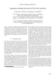
526 IEEE TRANSACTIONS ON CONTROL SYSTEMS TECHNOLOGY, VOL. 20, NO. 2, MARCH 2012Fig. 6. Experimental prototype schematic circuitry.Fig. 9. Functions implemented in the FPGA.Fig. 7. PV array electrical curves used the experimental tests.Fig. 10. Experimental Test 1.Fig. 8. Experimental prototype block diagram. Here k is a signal proportionalto A , i.e., k =(A )=(A), see Fig. 9.to generate fast changes in the PV array electrical characteristics.The curves programmed in the SAS for the experimentaltests performed are shown in Fig. 7. Due to the solararray simulator low output voltage level (it has a maximumvoltage of 80 V) a transformer was required to connect theGPV inverter prototype to the grid. As it can be seen in Fig. 6all the measurements where done in the low-voltage side ofthe transformer which exhibits a voltage amplitude of 31.4 Vat 50 Hz, and thus the transformer dynamics was not consideredin the model. Thus, for this experiment we considered thelow-voltage side of the transformer as the grid-voltage and measuredthe power factor in this side. In a larger version of thisprototype (with higher PV array’s voltage) the transformer canbe removed. A primary objective pursued when implementingthe controller was to obtain a simple, economical circuit. Thatis why we decided to divide the controller implementation in ananalog and digital stage. The analog stage has been designed to3 Even though we use a medium size, medium cost FPGA, the implementedalgorithm can be easily migrated to a cheaper PLD, e.g., CPLD or similar.Fig. 11. Experimental Test 2.generate the error signals, and , and the derivative of allowinga wider dynamic range than in most digital systems. Therest of the controller was implemented in a hardwired circuit,more specifically, a Xilinx Spartan three field-programmablegate array (FPGA). A hardwired programmable device is normallymore economical and faster than the equivalent microcontrolleror DSP. 3 The output signals of the analog module arethen quantized by means of ADC converters (ADC AD9525 of12 bits and 25 MSPS). The quantized signals are then inputtedto a digital processing stage implemented in a hardwired device,namely a Xilinx Spartan 3 FPGA. The hardwired algorithms implementedin the FPGA operates synchronously with a clock

MEZA et al.: LYAPUNOV-BASED CONTROL SCHEME FOR SINGLE-PHASE GRID-CONNECTED PV CENTRAL INVERTERS 527Fig. 12. Experimental Test 1. x ; x and v at 5 V/div; x at 1 A/div.Fig. 13. Experimental Test 2. x ; x and v at 5 V/div; x at 1 A/div.period of 4 ns. Additionally, the digital PWM that generates thesignals and is implemented within the FPGA using a sawtoothcarrier waveform with a period of 40.96 s. Fig. 8 showsa block diagram of the experimental setup implemented, noticethat as discussed in the previous section in order to simplify thecontroller is used instead of . Signal is assumed to begiven by an external MPPT. Fig. 9 shows the functions implementedin the FPGA. The following two different experimentaltests were performed.T1) Experimental Test 1: This experimental test deals withthe regulation of . The -averaged reference valueof the PV voltage, , is changed from 65 to 61 V andfinally arriving to the PV array maximum power pointvalue (57.2 V), as it is graphically shown in Fig. 10. Thereference value transitions were programmed to occurevery 60 grid cycles, i.e., 1.2 s.T2) Experimental Test 2: This test was designed to showthe adequate behavior of the closed-loop GPV inverterwhen abrupt changes in the electrical characteristics ofthe solar array simulator occur, emulating sudden irradiancechanges in the PV array. The solar array simulatorhas been programmed with two set of electrical

528 IEEE TRANSACTIONS ON CONTROL SYSTEMS TECHNOLOGY, VOL. 20, NO. 2, MARCH 2012characteristics, one corresponding to an irradiance of1000 Wm and another corresponding to an irradianceof 500 Wm . The experimental test consisted in thesudden change of the 1000 Wm electrical characteristicsset to the 500 Wm and then restoring the 1000Wm electrical characteristics set after a given time.This operation is shown in Fig. 11. This test is equivalentto an improvable worst case scenario and therefore itis a good way to validate the robustness of the designedcontroller.The values of the tunable parameters of the controller, i.e.,gains and , have been defined mainly to avoid numericalproblems (e.g., saturation of the signals, quantization problems).Therefore the gain has been chosen as large as possible butavoiding saturation of signal . The adaptive gain has beenchosen such that a smooth non-oscillating dynamics is obtained.The final values of gains used were and.Figs. 12 and 13 show the results of the aforementioned experimentaltests. In the case of Experimental Test 1 (see Fig. 12) itcan be seen that the output current is always in phase with thegrid voltage and that the capacitor voltage eventually reachesits desired steady-state value. The controller parameters havebeen intentionally set such that a smooth closed-loop voltagedynamics is obtained in order to avoid the introduction of unwantedharmonics in the output current, i.e., in single-phase PVpower inverters the effects of the voltage dynamics directly affectsthe output current.Fig. 13 shows the electrical behavior of the full-bridge inverterprototype with the designed control scheme for ExperimentalTest 2. Notice that when the abrupt step-down irradiancechange occurs ( 2.8 s), after a settling time approximatelyequal to 0.3 s, the system is able to reach the desired steady state.A similar settling time is obtained when the step-up irradiancechange occurs ( 7.05 s). Note that during the complete experimentaltest the current injected to the utility grid is always inphase with the grid voltage. It should be remarked that the differencein the response of during the step-down and step-upirradiance change is due to the nonlinear behavior of the system.The nonlinear behavior becomes more apparent in the presenceof large set-point changes, disturbances, or errors that cause thesystem to deviate from its nominal point of operation.VI. CONCLUSIONA novel approach to the controller design for single-phasesingle-stage grid-connected power inverters is presented. Insteadof linearizing the system, the control design approachaims to derive a global asymptotically stable closed-loopsystem that takes into account the nonlinear time-varying characteristicsof the system. The robustness of the controller hasbeen improved by adding an adaptive control law. A further theoreticalanalysis of the closed-loop system supported by meansof numerical simulations allows to simplify the implementationof the controller. A laboratory prototype was built in order totest the closed-loop performance of the controlled system. Theexperimental test performed consisted of an abrupt change ofthe PV array irradiance. Even though such sudden and largechange is not likely to occur in reality, it serves to underscorethe robustness and effectiveness of the proposed controller. Theexperimental results showed that the implemented controllerwas able to meet the desired control requirements, i.e., toextract a given amount of power from the PV array (solar arraysimulator, in the case of the experimental prototype) and toinject to the utility grid a current in phase with the grid voltageeven under extreme changes in the system parameters.The results of this paper should be considered as a proofof principle. It is expected that the proposed controller providesa similar performance as those obtained using standardlinear controller design techniques. Moreover, the inclusion ofthe nonlinear characteristics guarantees the closed-loop systemto operate robustly and reliable, even in the presence of largeset-point changes, disturbances, or errors that cause the systemto deviate from its nominal point of operation. It is our believethat further research in the design and analysis of PV power systemsconsidering and respecting their nonlinear nature may helpto obtain more efficient and reliable management and control algorithmsthan the ones currently available.REFERENCES[1] G. Petrone, G. Spagnuolo, R. Teodorescu, M. Veerachary, and M.Vitelli, “Reliability issues in photovoltaic power processing systems,”IEEE Trans. Ind. Electron., vol. 55, no. 7, pp. 2569–2580, Jul. 2008.[2] D. Zmood and D. Holmes, “Stationary frame current regulation ofPWM inverters with zero steady-state error,” IEEE Trans. PowerElectron., vol. 18, no. 3, pp. 814–822, May 2003.[3] R. Teodorescu, F. Blaabjerg, M. Liserre, and P. C. Loh, “Proportionalresonantcontrollers and filters for grid-connected voltage-source converters,”IEE Trans. Power Appl., vol. 153, no. 5, pp. 750–762, Sep.2006, 2006.[4] F. Blaabjerg, R. Teodorescu, M. Liserre, and A. V. Timubs, “Overviewof control and grid synchronization for distributed power generationsystems,” IEEE Trans. Ind. Electron., vol. 53, no. 5, pp. 1398–1409,Oct. 2006.[5] M. Ciobotaru, R. Teodorescu, and F. Blaabjerg, “Control of singlestagesingle-phase pv inverter,” in Proc. Eur. Conf. Power Electron.Appl., 2005, pp. 1–10.[6] C. Hua, J. Lin, and C. Shen, “Implementation of a dsp-controlled photovoltaicsystem with peak power tracking,” IEEE Trans. Ind. Electron.,vol. 45, no. 1, pp. 99–107, Feb. 1998.[7] M. Veerachary, T. Senjyu, and K. Uezato, “Voltage-based maximumpower point tracking control of PV system,” IEEE Trans. Aerosp. Electron.Syst., vol. 38, no. 1, pp. 262–270, Jan. 2002.[8] N. Femia, G. Petrone, G. Spagnuolo, and M. Vitelli, “Optimization ofperturb and observe maximum power point tracking method,” IEEETrans. Power Electron., vol. 20, no. 4, pp. 963–973, Jul. 2005.[9] R. Teodorescu, F. Blaabjerg, U. Borup, and M. Liserre, “A new controlstructure for grid-connected LCL PV inverters with zero steadystateerror and selective harmonic compensation,” in Proc. Appl. PowerElectron. Conf. Expo., 2004, pp. 580–586.[10] C.-Y. Chan, “A nonlinear control for DC-DC power converters,” IEEETrans. Power Electron., vol. 22, no. 1, pp. 216–222, Jan. 2007.[11] M. M. J. de Vries, M. J. Kransse, M. Liserre, V. G. Monopoli, and J. M.A. Scherpen, “Passivity-based harmonic control through series/paralleldamping of an h-bridge rectifier,” in Proc. Int. Symp. Ind. Electron.,2007, pp. 3385–3390.[12] D. Jeltsema and J. M. A. Scherpen, “A power-based perspective inmodeling and control of switched power converters [past and present],”IEEE Ind. Electron. Mag., vol. 1, no. 1, pp. 7–54, May 2007.[13] A. Gensior, H. Sira-Ramirez, J. Rudolph, and H. Guldner, “On somenonlinear current controllers for three-phase boost rectifiers,” IEEETrans. Ind. Electron., vol. 56, no. 2, pp. 360–370, Feb. 2009.[14] S. Sanders and G. Verghese, “Lyapunov-based control for switchedpower converters,” IEEE Trans. Power Electron., vol. 7, no. 1, pp.17–24, Jan. 1992.

MEZA et al.: LYAPUNOV-BASED CONTROL SCHEME FOR SINGLE-PHASE GRID-CONNECTED PV CENTRAL INVERTERS 529[15] R. Leyva, A. Cid-Pastor, C. Alonso, I. Queinnec, S. Tarbouriech, andL. Martinez-Salamero, “Passivity-based integral control of a boost converterfor large-signal stability,” IEE Proc. Control Theor. Appl., vol.153, no. 2, pp. 139–146, 2006.[16] H. Komurcugil and O. Kukrer, “A new control strategy for single-phaseshunt active power filters using a lyapunov function,” IEEE Trans. Ind.Electron., vol. 53, no. 1, pp. 305–312, Feb. 2006.[17] C. Meza, D. Jeltsema, D. Biel, and J. M. A. Scherpen, “Passive p-controlfor grid-connected PV systems,” in Proc. 17th IFAC World Congr.,2008, pp. 5575–5580.[18] G. Escobar, A. Stankovic, P. Mattavelli, F. Gordillo, and J. Aracil,“From adaptive PBC to PI nested control for SATCOM,” in Proc. IFACWorkshop Digit. Control, 2000, pp. 459–464.[19] G. Escobar, D. Chevreau, R. Ortega, and E. Mendes, “An adaptive passivity-basedcontroller for a unity power factor rectifier,” IEEE Trans.Control Syst. Technol., vol. 9, no. 4, pp. 637–644, Jul. 2001.[20] M. Calais, J. Myrzik, T. Spooner, and V. Agelidis, “Inverter for singlephasegrid connected photovoltaic systems—an overview,” in Proc.Power Electron. Specialists Conf., Feb. 2002, vol. 4, pp. 1995–2000.[21] S. B. Kjaer, J. K. Pedersen, and F. Blaabjerg, “A review of single-phasegrid-connected inverters for photovoltaic modules,” IEEE Trans. Ind.Appl., vol. 41, no. 5, pp. 1292–1306, Sep./Oct. 2005.[22] M. Meinhardt, “Past, present and future of grid connected photovoltaicand hybrid power systems,” in Proc. Power Eng. Soc. Summer Meet.,Jul. 2000, vol. 2, pp. 1283–1288.[23] S. Chiang, K. Chang, and Y. Yen, “Residential photovoltaic energystorage system,” IEEE Trans. Ind. Electron., vol. 45, no. 3, pp.385–394, Jun 1998.[24] D. Cruz-Martins and R. Demonti, “Photovoltaic energy processing forutility connected system,” in Proc. 27th Annu. Conf. IEEE Ind. Electron.Soc., 2001, pp. 1292–1296.[25] S. Busquets-Monge, J. Rocabert, P. Rodriguez, S. Alepuz, and J. Bordonau,“Multilevel diode-clamped converter for photovoltaic generatorswith independent voltage control of each solar array,” IEEE Trans.Ind. Electron., vol. 55, no. 7, pp. 2713–2723, Jul. 2008.[26] C. Meza, J. Negroni, D. Biel, and F. Guinjoan, “Inverter configurationcomparative for residential pv-grid connected systems,” in Proc. Int.Conf. Ind. Electron. IEEE, Nov. 2006, pp. 4361–4366.[27] J. A. Gow and C. D. Manning, “Development of a photovoltaic arraymodel for use in power-electronics simulation studies,” IEE Proceedings—Electr.Power Appl., vol. 146, no. 2, pp. 193–200, Mar. 1999.[28] S. Liu and R. Dougal, “Dynamic multi-physics model for solar array,”IEEE Trans. Ind. Electron., vol. 17, no. 2, pp. 285–294, Jun. 2002.[29] U. Boke, “A simple model of photovoltaic module electric characteristics,”in Proc. Eur. Conf. Power Electron. Appl., Sep. 2007, pp. 1–8.[30] R. Leyva, C. Alonso, I. Queinnec, A. Cid-Pastor, D. Lagrange, and L.Martinez-Salamero, “MPPT of photovoltaic systems using extremum- seeking control,” IEEE Trans. Aerosp. Electron. Syst., vol. 42, no. 1,pp. 249–258, Jan. 2006.[31] S. Jain and V. Agarwal, “Comparison of the performance of maximumpower point tracking schemes applied to single-stage grid-connectedphotovoltaic systems,” IET Electr. Power Appl., vol. 1, no. 5,pp. 753–762, Sep. 2007.