Discrete exterior geometry approach to structure-preserving ... - ITM

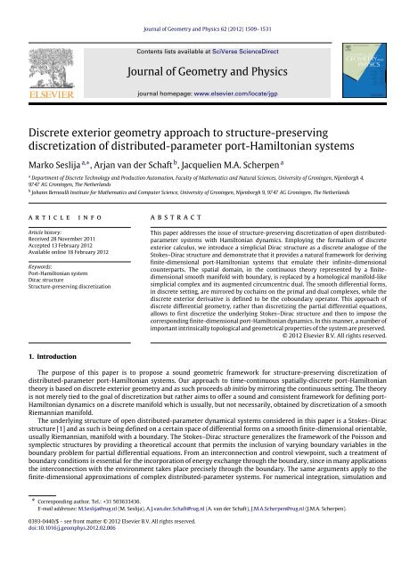
Journal of Geometry and Physics 62 (2012) 1509–1531Contents lists available at SciVerse ScienceDirectJournal of Geometry and Physicsjournal homepage: www.elsevier.com/locate/jgpDiscrete exterior geometry approach to structure-preservingdiscretization of distributed-parameter port-Hamiltonian systemsMarko Seslija a,∗ , Arjan van der Schaft b , Jacquelien M.A. Scherpen aa Department of Discrete Technology and Production Automation, Faculty of Mathematics and Natural Sciences, University of Groningen, Nijenborgh 4,9747 AG Groningen, The Netherlandsb Johann Bernoulli Institute for Mathematics and Computer Science, University of Groningen, Nijenborgh 9, 9747 AG Groningen, The Netherlandsa r t i c l ei n f oa b s t r a c tArticle history:Received 28 November 2011Accepted 13 February 2012Available online 18 February 2012Keywords:Port-Hamiltonian systemDirac structureStructure-preserving discretizationThis paper addresses the issue of structure-preserving discretization of open distributedparametersystems with Hamiltonian dynamics. Employing the formalism of discreteexterior calculus, we introduce a simplicial Dirac structure as a discrete analogue of theStokes–Dirac structure and demonstrate that it provides a natural framework for derivingfinite-dimensional port-Hamiltonian systems that emulate their infinite-dimensionalcounterparts. The spatial domain, in the continuous theory represented by a finitedimensionalsmooth manifold with boundary, is replaced by a homological manifold-likesimplicial complex and its augmented circumcentric dual. The smooth differential forms,in discrete setting, are mirrored by cochains on the primal and dual complexes, while thediscrete exterior derivative is defined to be the coboundary operator. This approach ofdiscrete differential geometry, rather than discretizing the partial differential equations,allows to first discretize the underlying Stokes–Dirac structure and then to impose thecorresponding finite-dimensional port-Hamiltonian dynamics. In this manner, a number ofimportant intrinsically topological and geometrical properties of the system are preserved.© 2012 Elsevier B.V. All rights reserved.1. IntroductionThe purpose of this paper is to propose a sound geometric framework for structure-preserving discretization ofdistributed-parameter port-Hamiltonian systems. Our approach to time-continuous spatially-discrete port-Hamiltoniantheory is based on discrete exterior geometry and as such proceeds ab initio by mirroring the continuous setting. The theoryis not merely tied to the goal of discretization but rather aims to offer a sound and consistent framework for defining port-Hamiltonian dynamics on a discrete manifold which is usually, but not necessarily, obtained by discretization of a smoothRiemannian manifold.The underlying structure of open distributed-parameter dynamical systems considered in this paper is a Stokes–Diracstructure [1] and as such is being defined on a certain space of differential forms on a smooth finite-dimensional orientable,usually Riemannian, manifold with a boundary. The Stokes–Dirac structure generalizes the framework of the Poisson andsymplectic structures by providing a theoretical account that permits the inclusion of varying boundary variables in theboundary problem for partial differential equations. From an interconnection and control viewpoint, such a treatment ofboundary conditions is essential for the incorporation of energy exchange through the boundary, since in many applicationsthe interconnection with the environment takes place precisely through the boundary. The same arguments apply to thefinite-dimensional approximations of complex distributed-parameter systems. For numerical integration, simulation and∗ Corresponding author. Tel.: +31 503633436.E-mail addresses: M.Seslija@rug.nl (M. Seslija), A.J.van.der.Schaft@rug.nl (A. van der Schaft), J.M.A.Scherpen@rug.nl (J.M.A. Scherpen).0393-0440/$ – see front matter © 2012 Elsevier B.V. All rights reserved.doi:10.1016/j.geomphys.2012.02.006

1510 M. Seslija et al. / Journal of Geometry and Physics 62 (2012) 1509–1531control synthesis, it is of paramount interest to have finite approximations that can be interconnected to one another or viathe boundary coupled to other systems, be they finite- or infinite-dimensional.Most of the numerical algorithms for spatial discretization of distributed-parameter systems, primarily finite differenceand finite element methods, fail to capture the intrinsic system structures and properties, such as symplecticity, conservationof momenta and energy, as well as differential gauge symmetry. Furthermore, some important results, including the Stokestheorem, fail to apply numerically and thus lead to spurious results. This loss of fidelity to preserve some inherent topologicaland geometric structures of the continuous models motivates a more geometry based approach.The discrete approach to geometry goes back to Whitney, who in [2] introduced an isomorphism between simplicialand de Rham cohomology. More recent antecedents can be found, for instance, in [3], and also in the computationalelectromagnetism literature [4–6]. For a comprehensive historical summary we refer to the thesis [7] and references therein.The literature, however, seems mostly focused on discretization of systems with infinite spatial domains, boundarylessmanifolds, and systems with zero boundary conditions. In this paper, we augment the definition of the dual cell complex inorder to allow nonzero energy flow through boundary.A notable previous attempt to resolve the problem of structure-preserving discretization of port-Hamiltonian systemsis [8], where the authors employ the mixed finite element method. Their treatment is restricted to the one-dimensionaltelegraph equation and the two-dimensional wave equation. Although it is hinted that the same methodology applies inhigher dimensions and to the other distributed-parameter systems, the results are not clear. It is worth noting that thechoice of the basis functions can have dramatic consequences on the numerical performance of the mixed finite elementmethod; as the mesh is being refined, it easily may lead to an ill-conditioned finite-dimensional linear system [9]. The otherundertaking on discretization of port-Hamiltonian systems can be found in [10,11], but the treatment is purely topologicaland is more akin to the graph-theoretical formulation of conservation laws. Furthermore, the authors in [10,11] do notintroduce a discrete analogue of the Stokes theorem and the entire approach is tied to the goal of preserving passivity.Our approach is that of discrete exterior calculus [12,13,7,14], which has previously been applied to variational problemsnaturally arising in mechanics and electromagnetism. These problems stem from a Lagrangian, rather than Hamiltonian,modeling perspective and as such they conform to a multisymplectic structure [15–18], rather than the Stokes–Diracstructure. A crucial ingredient for the numeric integration is the asynchronous variational integrator for spatio-temporallydiscretized problems, whereas our approach spatially discretizes the Stokes–Dirac structure and allows imposing timecontinuousspatially discrete dynamics. This apparent discrepancy between multisymplectic and the Stokes–Dirac structurepreservingdiscretization could be elevated by, for instance, defining Stokes–Dirac structure on a pseudo-Riemannianmanifold to insure a treatment of space and time on equal footing, whilst keeping nonzero exchange through theboundary.Contribution and outline of the paper. We begin by recalling the definition of the Stokes–Dirac structure and port-Hamiltoniansystems. In order to make this paper as self-contained as possible for a variety of readers, we present a brief overview ofthe elementary discrete exterior geometry needed to define a discretized Stokes–Dirac structure and impose appropriateport-Hamiltonian dynamics. The third section is a brief summary of the essential definitions and results in discrete exteriorcalculus as developed in [12,13,7]. The contribution of this paper in this regard is a proper treatment of the boundary of thedual cell complex. Namely, in order to allow the inclusion of nonzero boundary conditions on the dual cell complex, we offera definition of the dual boundary operator that differs from the standard one. Such a construction leads to a discrete analogueof the integration by parts formula, which is a crucial ingredient in establishing a discrete Stokes–Dirac structure on a primalsimplicial complex and its circumcentric dual. The main result is presented in Section 4, where we introduce the notion ofsimplicial Dirac structures on a primal–dual cell complex, and in the following section define port-Hamiltonian systems withrespect to these structures. In Section 6 we give a matrix representation for the simplicial Dirac structures and linear port-Hamiltonian systems, for which we also establish bounds for the energy of discretization errors. Finally, we demonstrate howthe simplicial Dirac structures relate to some spatially discretized distributed-parameter systems with boundary variables:Maxwell’s equations on a bounded domain, a two-dimensional wave equation, and the telegraph equations. While the focusof this paper is not implementation of discrete exterior calculus in discretization of port-Hamiltonian systems, we have,nonetheless, taken some preliminary numerical investigations. We demonstrate the application of the developed machineryusing the example of the telegraph equations.Some preliminary results of this paper have been reported in [19].2. Dirac structures and port-Hamiltonian dynamicsDirac structures were originally developed in [20–22] as a generalization of symplectic and Poisson structures.The formalism of Dirac structure was employed as the geometric notion underpinning generalized power-conservinginterconnections and thus allowing the Hamiltonian formulation of interconnected and constrained dynamical systems.A constant Dirac structure can be defined as follows. Let F , E, and L be linear spaces. Given a f ∈ F and an e ∈ E, thepairing will be denoted by ⟨e|f ⟩ ∈ L. By symmetrizing the pairing, we obtain a symmetric bilinear form ⟨⟨, ⟩⟩ : F × E → Ldefined by⟨⟨(f 1 , e 1 ), (f 2 , e 2 )⟩⟩ = ⟨e 1 |f 2 ⟩ + ⟨e 2 |f 1 ⟩.

M. Seslija et al. / Journal of Geometry and Physics 62 (2012) 1509–1531 1511Definition 2.1. A Dirac structure is a linear subspace D ⊂ F × E such that D = D ⊥ , with ⊥ standing for the orthogonalcomplement with respect to the bilinear form ⟨⟨, ⟩⟩.It immediately follows that for any (f , e) ∈ D0 = ⟨⟨(f , e), (f , e)⟩⟩ = 2⟨e|f ⟩.Interpreting (f , e) as a pair of power variables, the condition (f , e) ∈ D implies power-conservation ⟨e|f ⟩ = 0, and as suchis terminus a quo for the geometric formulation of port-Hamiltonian systems.Much is known about finite-dimensional Dirac structures and their role in physics; however, hitherto there is no completetheory of Dirac structures for field theories. An initial contribution in this direction is made in the paper [1], where the authorsintroduce a notion of the Stokes–Dirac structure. This infinite-dimensional Dirac structure lays down the foundation for port-Hamiltonian formulation of a class of distributed-parameter systems with boundary energy flow. In this section, we providea very brief overview of the Stokes–Dirac structure [1].Throughout this paper, let M be an oriented n-dimensional smooth manifold with a smooth (n−1)-dimensional boundary∂M endowed with the induced orientation, representing the space of spatial variables. By Ω k (M), k = 0, 1, . . . , n, denotethe space of exterior k-forms on M, and by Ω k (∂M), k = 0, 1, . . . , n − 1, the space of k-forms on ∂M. A natural nondegenerativepairing between α ∈ Ω k (M) and β ∈ Ω n−k (M) is given by ⟨β|α⟩ = β ∧ α. Likewise, the pairing on theMboundary ∂M between α ∈ Ω k (∂M) and β ∈ Ω n−k−1 (∂M) is given by ⟨β|α⟩ = β ∧ ∂M α.For any pair p, q of positive integers satisfying p + q = n + 1, define the flow and effort linear spaces byF p,q = Ω p (M) × Ω q (M) × Ω n−p (∂M)E p,q = Ω n−p (M) × Ω n−q (M) × Ω n−q (∂M).The bilinear form on the product space F p,q × E p,q is given by⟨⟨(f 1 , p f 1 , q f 1b, e 1 , p e1, q e1 b), (f 2 , p f 2 , q f 2 , b e2, p e2, q e2)⟩⟩b∈F p,q ∈E p,q= ⟨e 1 ∧ p f 2 + p e1 ∧ q f 2 + q e2 ∧ p f 1 + p e2 ∧ q f 1 , M⟩ + q ⟨e1 ∧ b f 2 + b e2 ∧ b f 1b, ∂M⟩. (2.1)Theorem 2.1. Given linear spaces F p,q and E p,q , and bilinear form ⟨⟨, ⟩⟩, define the following linear subspace D of F p,q × E p,q fp 0 (−1)D = (f p , f q , f b , e p , e q , e b ) ∈ F p,q × E p,q =pq+1 d ep,f q d 0 e q fb 1 0 ep |=∂Me b 0 −(−1) n−q , (2.2)e q | ∂Mwhere d is the exterior derivative and | ∂M stands for a trace on the boundary ∂M. Then D = D ⊥ , that is, D is a Dirac structure.Remark 2.1. Although the differential operator in (2.2), in the presence of nonzero boundary conditions, is not skewsymmetric,it is possible to associate a pseudo-Poisson structure to the Stokes–Dirac structure [1]. In the absence ofalgebraic constraints, the Stokes–Dirac structure specializes to a Poisson structure [22], and as such it can be derived throughsymmetry reduction from a canonical Dirac structure on the phase space [23]. Whether this reduction can be done for theStokes–Dirac structure on a manifold with boundary remains an important open problem.In order to define Hamiltonian dynamics, consider a Hamiltonian density H : Ω p (M) × Ω q (M) → Ω n (M) resultingwith the Hamiltonian H = H ∈ M R. Now, consider a time function t → (α p(t), α q (t)) ∈ Ω p (M) × Ω q (M), t ∈ R, andthe Hamiltonian t → H(α p (t), α q (t)) evaluated along this trajectory, then at any tdHdt=Mδ p H ∧ ∂α p∂t+ δ q H ∧ ∂α q∂t ,where (δ p H, δ q H) ∈ Ω n−p (M) × Ω n−q (M) are the (partial) variational derivatives of H at (α p , α q ).Setting the flows f p = − ∂α p, f ∂t q = − ∂α qand the efforts e∂tp = δ p H, e q = δ q H, the distributed-parameter port-Hamiltoniansystem is defined by the relation− ∂α p∂t , − ∂α q∂t , f b, δ p H, δ q H, e b ∈ D, t ∈ R.For such a system, it straightaway follows that dH = dt ∂M e b ∧ f b , expressing the fact that the system is lossless. In otherwords, the increase in the energy of the system is equal to the power supplied to the system through the boundary ∂M.

1512 M. Seslija et al. / Journal of Geometry and Physics 62 (2012) 1509–15313. Fundamentals of discrete exterior calculusThe discrete manifolds we employ are oriented manifold-like simplicial complexes and their circumcentric duals.Typically, these manifolds are simplicial approximations of smooth manifolds. Familiar examples are meshes of trianglesembedded in R 3 and tetrahedra obtained by tetrahedrization of a 3-dimensional manifold. There are many ways to obtainsuch complexes; however, we do not address the issue of discretization and embedding.As said, we proceed ab initio and mostly our treatment is purely formal, that is without proofs that the discrete objectsconverge to the continuous ones, though we briefly address the issue of convergence in Section 6.3. By construction ofdiscrete exterior calculus, a number of important geometric structures are preserved and propositions like the Stokestheorem are true by definition. The basic building blocks of discrete exterior geometry are discrete chains and cochains,and their geometric duals. The former are simplices and the latter are discrete differential forms related one to another bybilinear pairing that can be understood as the evaluation of a cochain on an appropriate simplex, and as such parallels theintegration in the continuous setting.In discrete exterior calculus, a dual mesh is instrumental for defining the diagonal Hodge star. In the paper at hand, thegeometric duality is a crucial ingredient in establishing a bijective relationship between the flow and effort spaces, as wellas for construction of nondegenerate discrete analogues of the bilinear form (2.1).This section, with some modification concerning the treatment of the boundary of the dual cell complex, is a briefsummary of the essential definitions and results in discrete exterior calculus as developed in [12,13,7]. As therein, firstwe define discrete differential forms, the discrete exterior derivative, the codifferential operator, the Hodge star, and thediscrete wedge product. For more information on the construction of the other discrete objects such as vector fields, adiscrete Lie derivative, and discrete musical operators, we refer the reader to [7]. Construction of all these discrete objectsis in a way simpler than their continuous counterparts since we require only a local metric, ergo the machinery of theRiemannian geometry is not demanded. With the exception of the treatment of the notions related the boundary of the dualcell complex, a good part of this section is a recollection of the basic concepts and results of algebraic topology [24,25].3.1. Simplicial complexes and their circumcentric dualsDefinition 3.1. A k-simplex is the convex span of k + 1 geometrically independent points, k nσ k = [v 0 , v 1 , . . . , v k ] = α i v i | α i ≥ 0, α i = 1 .i=0i=0The points v 0 , . . . , v k are called the vertices of the simplex, and the number k is called the dimension of the simplex. Anysimplex spanned by a (proper) subset of {v 0 , . . . , v k } is called a (proper) face of σ k . If σ l is a proper face of σ k , we denotethis by σ l ≺ σ k .As an illustration, consider four non-collinear points v 0 , v 1 , v 2 , and v 3 in R 3 . Each of these points individually is 0-simplexwith an orientation dictated by the choice of a sign. An example of a 1-simplex is a line segment [v 0 , v 1 ] oriented from v 0to v 1 . The triangle [v 0 , v 1 , v 2 ] is an example of 2-simplex oriented in counterclockwise direction. Similarly, the tetrahedron[v 0 , v 1 , v 2 , v 3 ] is a 3-simplex.Definition 3.2. A simplicial complex K in R N is a collection of simplices in R N , such that:(1) Every face of a simplex of K is in K .(2) The intersection of any two simplices of K is a face of each of them.The dimension n of the highest dimension simplex in K is the dimension of K .The above given definition of a simplicial complex is more general than needed for the purposes of exterior calculus. Sincethe discrete theory employed in this paper mirrors the continuous framework, we restrict our considerations to manifold-likesimplicial complexes [7].Definition 3.3. A simplicial complex K of dimension n is a manifold-like simplicial complex if the underlying space is apolytope |K|. In such a complex all simplices of dimension k = 0, . . . , n − 1 must be a face of some simplex of dimension nin the complex.Introducing these simplicial meshes has an added advantage of allowing a simple and intuitive definition of orientabilityof simplicial complexes [7].Definition 3.4. An n-dimensional simplicial complex K is an oriented manifold-like simplicial complex if the n-simplicesthat share a common (n − 1)-face have the same orientation and all the simplices of lower dimensions are individuallyoriented.

1514 M. Seslija et al. / Journal of Geometry and Physics 62 (2012) 1509–1531Definition 3.5. Let K be a simplicial complex. We denote the free Abelian group generated by a basis consisting of orientedk-simplices by C k (K; Z). This is the space of finite formal sums of the k-simplices with coefficients in Z. Elements of C k (K; Z)are called k-chains.Definition 3.6. A primal discrete k-form α is a homomorphism from the chain group C k (K; Z) to the additive group R. Thus,a discrete k-form is an element of Hom(C k (K), R), the space of cochains. This space becomes an Abelian group if we add twohomomorphisms by adding their values in R. The standard notation for Hom(C k (K), R) in algebraic topology is C k (K; R);however, like in [12,13,7] we shall also employ the notation Ω k d(K) for this space as a reminder that this is the space ofdiscrete k-forms on the simplicial complex K . Thus,Ω k d (K) := C k (K; R) = Hom(C k (K), R). Given a k-chaini a ic k, i a i ∈ Z, and a discrete k-form α, we have α a i c k i= a i α(c k ), iiiand for two discrete k-forms α, β ∈ Ω k d (K) and a k-chain c ∈ C k(K; Z),(α + β)(c) = α(c) + β(c).The natural pairing of a k-form α and a k-chain c is defined as the bilinear pairing ⟨α, c⟩ = α(c).As previously pointed out, a differential k-form α k can be thought of as a linear functional that assigns a real number toeach oriented cell σ k ∈ K . In order to understand the process of discretization of the continuous problem consider a smoothk-form f ∈ Ω k (|K|). The discrete counterpart of f on a k-simplex σ k ∈ K is a discrete form α k defined as α(σ k ) := σ k f .Definition 3.7. The boundary operator ∂ k : C k (K; Z) → C k−1 (K; Z) is a homomorphism defined by its action on a simplexσ k = [v 0 , . . . , v k ],∂ k σ k = ∂ k ([v 0 , . . . , v k ]) =k(−1) i [v 0 , . . . , ˆv i , . . . , v k ],i=0where [v 0 , . . . , ˆv i , . . . , v k ] is the (k − 1)-simplex obtained by omitting the vertex v i . Note that ∂ k ◦ ∂ k+1 = 0.Definition 3.8. On a simplicial complex of dimension n, a chain complex is a collection of chain groups and homomorphisms∂ k , such that0 −→ C n (K) ∂ n ∂ n−1 ∂ k+1−→ C n−1 −−→ · · · −−→ Ck (K) ∂ k−→ · · · −→ ∂1C 0 (K) ∂ 0−→ 0,and ∂ k ◦ ∂ k+1 = 0.Definition 3.9. The discrete exterior derivative d : Ω k k+1d(K) → Ωd(K) is defined by duality to the boundary operator∂ k+1 : C k+1 (K; Z) → C k (K; Z), with respect to the natural pairing between discrete forms and chains. For a discrete formα k ∈ Ω k(K) d and a chain c k+1 ∈ C k+1 (K; Z) we define d by⟨dα k , c k+1 ⟩ = ⟨α k , ∂ k+1 c k+1 ⟩.The discrete exterior derivative is the coboundary operator from algebraic topology [25] and as such it induces the cochaincomplex0 ←− Ω n d (K) d ←− Ω n−1dwhere d ◦ d = 0.d←− · · ·d←− Ω 0 d(K) ←− 0,Such as in the continuous theory, we drop the index of the boundary operator when its dimension is clear from thecontext. The discrete exterior derivative d is constructed in such a manner that the Stokes theorem is satisfied by definition.This means, given a (k + 1)-chain c and a discrete k-form α, the discrete Stokes theorem states that⟨dα, c⟩ = ⟨α, ∂c⟩. Consider a k-chaini a ic i , a i ∈ Z, c i ∈ C k (K; Z), and (k − 1)-form α ∈ Ω k−1d(K; Z). By linearity of the chain–cochainpairing, the discrete Stokes theorem can be stated asdα, a i c i = α, ∂ a i c i = α, a i ∂c i = a i ⟨α, ∂c i ⟩ .iiii

M. Seslija et al. / Journal of Geometry and Physics 62 (2012) 1509–1531 1515As in the continuous setting, the discrete wedge product pairs two discrete differential forms by building a higher degreeform. The primal–primal wedge product inherits some important properties of the cup product such as the bilinearity,anticommutativity and naturality under pull-back [12,7]; however, it is in general non-associative and degenerate, and thusunsuitable for construction of canonical pairing between the flow and effort space. For a definition of nondegenerate pairingbetween the flow and effort discrete forms we shall use a primal–dual wedge product as will be defined in the subsequentsection.3.3. Metric-dependent part of discrete exterior calculusA cellular chain group associated with the dual cell complex D(K), in [25] denoted by D p (K), is the group of formalsums of cells with integer coefficients. Since in D(K) the information of dual simplices is lost, to retain the bookkeepinginformation Hirani in [7] introduces a duality operator which takes values in the domain group C p (csd K; Z). As will be clearfrom the subsequent section, this bookkeeping is not indispensable for the formulation of the Dirac structure on a simplicialcomplex; nevertheless, since the information of dual simplices might be needed in defining dynamics, we also employ thisconstruction.In order to explicitly construct the duality on the boundary, in the next definition we introduce the boundary staroperator. Shortly afterward we shall explain the rational behind this construction.Definition 3.10. Let K be a well-centered simplicial complex of dimension n. The interior circumcentric duality operator⋆ i : C k (K; Z) → C n−k (csd K; Z)⋆ i (σ k ) =s σ k ,...,σ c(σ k n ), c(σ k+1 ), . . . , c(σ n ) ,σ k ≺σ k+1 ≺···≺σ nand the boundary star operator ⋆ b : C k (∂K; Z) → C n−1−k (∂(csd K); Z)⋆ b (σ k ) =s σ k ,...,σ c(σ k n−1 ), c(σ k+1 ), . . . , c(σ n−1 ) ,σ k ≺σ k+1 ≺···≺σ n−1where the s σ k ,...,σ n and s σ k ,...,σ n−1 coefficients ensure that the orientation of the cell [c(σ k ), c(σ k+1 ), . . . , c(σ n )] and[c(σ k ), c(σ k+1 ), . . . , c(σ n−1 )] is consistent with the orientation of the primal simplex, and the ambient volume forms on Kand ∂K , respectively.The subset of chains C p (csd K; Z) that are equal to the cells of D(K)×D(∂K) forms a subgroup of C p (csd K; Z). We denotethis subgroup of C p (csd K; Z) by C p (⋆K; Z), where ⋆K is its basis set. A cell complex ⋆K in R N is a collection of cells in R Nsuch that: (1) there is a partial ordering of cells in ⋆K, ˆσ k ≺ ˆσ l , which is read as ˆσ k is a face of ˆσ l ; (2) the intersection of anytwo cells in ⋆K , is either a face of each of them, or it is empty; (3) the boundary of a cell is expressed as a sum of its properfaces.Given a simplicial well-centered complex K , we define its interior dual cell complex ⋆ i K (block complex in terminology ofalgebraic topology [25]) as a circumcentric dual restricted to |K|. An important property of the Voronoi duality is that primaland dual cells are orthogonal to each other. The boundary dual cell complex ⋆ b K is a dual to ∂K . The dual cell complex ⋆Kis defined as ⋆K = ⋆ i K × ⋆ b K . A dual mesh ⋆ i K is a dual to K in sense of a graph dual, and the dual of the boundary isequal to the boundary of the dual, that is ∂(⋆K) = ⋆(∂K) = ⋆ b K . This construction of the dual is compatible with [14,26]and as such is very similar to the use of the ghost cells in finite volume methods in order to account for the duality relationbetween the Dirichlet and the Neumann boundary conditions. Because of duality, there is a one-to-one correspondencebetween k-simplices of K and interior (n − k)-cells of ⋆K . Likewise, to every k-simplex on ∂K there is a uniquely associated(n − 1 − k)-cell on ∂(⋆K).In what follows, we shall abuse notation and use the same symbol ⋆ for both the interior circumcentric and the boundarystar operator. The difference, if not clear from the exposition, will be delineated by indicating that ⋆σ k ∈ ∂(⋆K) when ⋆σ kis a dual cell on the boundary of the dual cell complex ⋆K . As sets, the set of ¯D(σ p) and ⋆σ p are equal, the only differencebeing in the bookkeeping, since in ⋆σ p one retains the information about the simplices it is built of. Here we do not addressthe problem of the orientation of dual ⋆K , for which we direct the reader to [7]. The circumcentric dual cell complex of the2-dimensional simplicial complex from Fig. 1 is pictured in Fig. 2.An important concept in defining a wedge product between primal and dual cochains is the notion of a support volumeassociated with a given simplex or cell.Definition 3.11. The support volume of a simplex σ k is an n-volume given by the convex hull of the geometric union of thesimplex and its circumcentric dual. This is given byV σ k = CH(σ k , ⋆ i σ k ) ∩ |K|,where CH(σ k , ⋆ i σ k ) is the n-dimensional convex hull generated by σ k ∪ ⋆ i σ k . The intersection with |K| is necessary toensure that the support volume does not extend beyond the polytope |K| which would otherwise occur if K is nonconvex.

1516 M. Seslija et al. / Journal of Geometry and Physics 62 (2012) 1509–1531Fig. 2. The circumcentric dual cell complex ⋆K of the simplicial complex K given in Fig. 1. The boundary of ⋆K is the dual of the boundary of K . Somesupport volumes are shaded. For instance, the support volume of the primal vertex v r is the area of its Voronoi region; also V [vi ,v j ] = V ¯D([vi ,v j ]) .The support volume of a dual cell ⋆ i σ k isV ⋆i σ k = CH(⋆ i σ k , ⋆ i ⋆ i σ k ) ∩ |K| = V σ k.Everything that has been said about the primal chains and cochains can be extended to dual cells and dual cochains. Wedo not elaborate on this since it can be found in the literature [7,13], however, in order to properly account for the behaviorson the boundary, we need to adapt the definition of the boundary dual operator as presented in [7,13]. We propose thefollowing definition.Definition 3.12. The dual boundary operator ∂ k : C k (⋆ i K; Z) → C k−1 (⋆K; Z) is a homomorphism defined by its action on adual cell ˆσ k = ⋆ i σ n−k = ⋆ i [v 0 , . . . , v n−k ],where∂ ˆσ k = ∂ ⋆ i [v 0 , . . . , v n−k ] = ∂ i ⋆ i [v 0 , . . . , v n−k ] + ∂ b ⋆ i [v 0 , . . . , v n−k ],∂ i ⋆ i [v 0 , . . . , v n−k ] =σ n−k+1 ≻σ n−k ⋆ i (s σ n−k+1σ n−k+1 )∂ b ⋆ i [v 0 , . . . , v n−k ] = ⋆ bsσ n−kσ n−k .Note that the dual boundary operator as defined in [7] is equal to ∂ i . Hence, the dual boundary is not the geometric boundaryof a cell, because near the boundary of a manifold that would be wrong. As an example consider the complex in Fig. 3. Thedual of the vertex v 1 is the Voronoi region shown shaded. Its geometric boundary has five sides (two half primal edgesand three dual edges), whereas the dual boundary according to the definition given in [7] consists of just dual edges,i.e. [c([v 0 , v 1 ]), c([v 0 , v 1 , v 2 ])], [c([v 0 , v 1 , v 2 ]), c([v 1 , v 3 , v 2 ])] and [c([v 1 , v 3 , v 2 ]), c([v 1 , v 3 ])], all up to a sign dependingon the chosen orientation. However, according to the above given definition, the boundary is comprised of four edges,three already given plus the boundary edge [c([v 0 , v 1 ]), c([v 1 , v 3 ])] obtained by aggregation of the two dual simplices[c([v 0 , v 1 ]), v 1 ] and [v 1 , c([v 1 , v 3 ])]. This construction of the dual boundary ensures a natural pairing between a primal0-form defined on v 1 and a dual 1-form on [c([v 0 , v 1 ]), c([v 1 , v 3 ])]. The offered definition of the dual boundary operator, aswill be demonstrated later, is crucial for the inclusion of the boundary variables in the discrete setting.Definition 3.13. The dual discrete exterior derivative d : Ω k k+1d(⋆K) → Ωd(⋆ i K) is defined by duality to the boundaryoperator ∂ : C k+1 (⋆ i K; Z) → C k (K; Z). For a dual discrete form ˆα k ∈ Ω k(⋆K) d and a chain ĉ k+1 ∈ C k+1 (⋆ i K; Z) we define dby⟨d ˆα k , ĉ k+1 ⟩ = ⟨ ˆα k , ∂ĉ k+1 ⟩.The dual discrete exterior derivative d can be decomposed into the two operators d i and d b , which are respectively dual to∂ i and ∂ i , that is⟨d ˆα k , ĉ k+1 ⟩ = ⟨d i ˆα k , ĉ k+1 ⟩ + ⟨d b ˆα k , ĉ k+1 ⟩ = ⟨ ˆα k , ∂ i ĉ k+1 ⟩ + ⟨ ˆα k , ∂ b ĉ k+1 ⟩.The support volumes of a simplex and its dual cell are the same, which suggests that there is a natural identificationbetween primal k-cochains and dual (n − k)-cochains.

M. Seslija et al. / Journal of Geometry and Physics 62 (2012) 1509–1531 1517Fig. 3. A 2-dimensional simplicial complex taken from Fig. 3.3, Section 3.6, [7]. The shaded region is a Voronoi dual of the primal vertex v 1 . The dualboundary, according to [7], is not the geometric boundary near the boundary of the manifold. However, in line with our construction, the boundary of thedual is the dual of the boundary.In the exterior calculus for smooth manifolds, the Hodge star, denoted ∗, is an isomorphism between the space of k-formsand (n − k)-forms. Since the Hodge star operator is metric-dependent, in the discrete theory, it is defined as an equality ofaverages between primal and their dual forms [7,27].Definition 3.14. The discrete Hodge star is a map ∗ : Ω k n−kd(K) → Ωd(⋆ i K) defined by its value over simplices and theirduals. For a k-simplex σ k , and a discrete k-form α k ,1| ⋆ i σ k | ⟨∗αk , ⋆ i σ k ⟩ = s 1|σ k | ⟨αk , σ k ⟩,where s is ±1 (see [7]).Similarly we can define the discrete Hodge operator on the boundary, that is on an (n−1)-dimensional simplicial complexand its dual. It is trivial to show that for a k-form α k the following holds: ∗ ∗ α k = (−1) k(n−k) .Remark 3.2. The discrete Hodge star can be represented by a matrix (see Section 6). According to Definition 3.14, this matrixis diagonal. In the case Whitney forms are used, the discrete Hodge operator is sparse but not diagonal in general [27].Next, we define a natural pairing, via so-called primal–dual wedge product, between a primal k-cochain and a dual (n−k)-cochain. The resulting discrete form is the volume form. In order to insure anticommutativity of the primal–dual wedgeproduct, we take the following definition.Definition 3.15. Let α k ∈ Ω k(K) d be a primal k-form and ˆβ n−k ∈ Ω n−kd(⋆ i K). We define the discrete primal–dual wedgeproduct ∧ : Ω k n−kd(K) × Ωd(⋆ i K) → Ω n d (V k(K)) by n⟨α k ∧ ˆβ n−k |V, V σ k⟩ =σ k|k |σ k | | ⋆ i σ k | ⟨αk , σ k ⟩⟨ ˆβ n−k , ⋆ i σ k ⟩= ⟨α k , σ k ⟩⟨ ˆβ n−k , ⋆ i σ k ⟩= (−1) k(n−k) ⟨ ˆβ n−k ∧ α k , V σ k⟩,where V σ k is the n-dimensional support volume obtained by taking the convex hull of the simplex σ k and its dual ⋆ i σ k .As an illustration, consider the two-dimensional simplicial complex K depicted in Fig. 1 and its dual ⋆K in Fig. 2. Letα 1 ∈ Ω 1 d (K) and ˆβ 1 ∈ Ω 1 d (⋆K). The dual cell of the primal edge [v k, v i ] is [ˆv m , ˆv m−1 ], up to a sign depending on the chosenorientation. The primal–dual wedge product of α 1 and ˆβ 1 on the support volume V [vk ,v i ] = V [ˆvm ,ˆv m−1 ], represented by thediamond shaped region generated by [v k , v i ] and [ˆv m , ˆv m−1 ], is simply a dot product α([v k , v i ]) · ˆβ 1 ([ˆv m , ˆv m−1 ]). Now, inorder to look at the primal–dual wedge product on the boundary, let γ 0 ∈ Ω 0(∂K) d and ˆη1 ∈ Ω 1 d(∂(⋆K)). For instance, ˆη1can be a restriction of ˆβ 1 on the boundary ∂(⋆K). The primal–dual wedge product ⟨γ 0 ∧ ˆη 1 , V vk ⟩ = γ 0 (v k ) · ˆη 1 ([ˆv p , ˆv p−1 ]).The volume for V vk = V [ˆvp ,ˆv p−1 ] is simply the measure of the cell [ˆv p , ˆv p−1 ].Here we note the advantage of employing circumcentric with respect to barycentric dual since one needs to store onlyvolume information about primal and dual cells, and not about the primal–dual convex hulls.Definition 3.16. Given two primal discrete k-forms, α k , β k ∈ Ω k d (K), their discrete L2 inner product, ⟨α k , β k ⟩ d is given by n⟨α k , β k |V⟩ d =σ k|k |σ k | | ⋆ i σ k | ⟨αk , σ k ⟩⟨∗β k , ⋆ i σ k ⟩= ⟨α k , σ k ⟩⟨∗β k , ⋆ i σ k ⟩.

1518 M. Seslija et al. / Journal of Geometry and Physics 62 (2012) 1509–1531The proposed definition of the dual boundary operator assures the validity of the summation by parts relation thatparallels the integration by parts formula for smooth differential forms.Proposition 3.1. Let K be an oriented well-centered simplicial complex. Given a primal (k − 1)-form α k−1 and a dual (n − k)-discrete form ˆβ n−k , then⟨dα k−1 ∧ ˆβ n−k , K⟩ + (−1) k−1 ⟨α k−1 ∧ d ˆβ n−k , K⟩ = ⟨α k−1 ∧ ˆβ n−k , ∂K⟩,where in the boundary pairing α k−1 is a primal (k − 1)-form on ∂K , while ˆβ n−k is a dual (n − k)-cochain taken on the boundarydual ⋆(∂K).Proof. We haveand⟨dα k−1 ∧ ˆβ n−k , K⟩ =σ k−1 ∈K= σ k−1 ∈K= σ k−1 ∈K⟨dα k−1 , σ k ⟩⟨ ˆβ n−k , ⋆ i σ n−k ⟩⟨α k−1 , ∂σ k ⟩⟨ ˆβ n−k , ⋆ i σ n−k ⟩σ k−1 ≺σ k ⟨α k−1 , σ k ⟩⟨ ˆβ n−k , ⋆ i σ n−k ⟩,⟨α k−1 ∧ d ˆβ n−k , K⟩ = σ k−1 ⟨α k−1 , σ k−1 ⟩⟨d ˆβ n−k , ⋆ i σ k−1 ⟩ = σ k−1 ⟨α k−1 , σ k−1 ⟩⟨ ˆβ n−k , ∂(⋆ i σ k−1 )⟩= σ k−1 ⟨α k−1 , σ k−1 ⟩ σ k−1 ≺σ k ⟨ ˆβ n−k , ⋆ i (s σ kσ k )⟩ + ⟨ ˆβ n−k , ⋆ b (s σ k−1σ k−1 )⟩Inducing the orientation of the dual such that s σ k = s σ k−1 = (−1) k completes the proof.ˆβRemark 3.3. Decomposing the dual form ˆβ n−k into the internal and the boundary part as ˆβ n−k = i ∈ Ω n−k (⋆ d i K) on ⋆ i Kˆβ b ∈ Ω n−k (⋆ d b K) on ∂(⋆K) anddecomposing the dual exterior derivative in the same manner, the summation by parts formula can be written as⟨dα k−1 ∧ ˆβ i , K⟩ + (−1) k−1 ⟨α k−1 ∧ (d i ˆβ i + d b ˆβ b ), K⟩ = ⟨α k−1 ∧ ˆβ b , ∂K⟩. (3.1)□.In the standard literature of discrete exterior calculus, the codifferential operator is adjoint to the discrete exteriorderivative, with respect to the inner products of discrete forms [7]. According to Proposition 3.1, this is not the case since onthe right a term corresponding to the primal–dual pairing on the boundary appears. As the subsequent section demonstrates,this term is precisely responsible for the inclusion of the boundary variables in the discretized Stokes–Dirac structure.4. Dirac structures on a simplicial complexThe Stokes–Dirac structure, which captures a differential symmetry of the Hamiltonian field equations, as presentedin [1], is metric-independent. The essence of its construction lies in the antisymmetry of the wedge product and the Stokestheorem. In a discrete framework, the primal–primal wedge product [7] inherits a number of important properties of thecup product [25], such as bilinearity, anti-commutativity and naturality under pullback; however, it is degenerate and thusunsuitable for defining a Dirac structure. This motivates a formulation of a Dirac structure on a simplicial complex and itsdual. We introduce Dirac structures with respect to the bilinear pairing between primal and duals forms on the underlyingdiscrete manifold. We call these Dirac structures simplicial Dirac structures.In the discrete setting, the smooth manifold M is replaced by an n-dimensional well-centered oriented manifold-likesimplicial complex K . The flow and the effort spaces will be the spaces of complementary primal and dual forms. Theelements of these two spaces are paired via the discrete primal–dual wedge product. Since the Stokes–Dirac structure Dexpresses the coupling between f p and e q , also f q and e p , via the exterior derivative, whose discrete analogue maps primalinto primal and dual into dual cochains, the flow space cannot be entirely built on a primal simplicial complex and the effortspace on a dual cell complex, or vice versa. Instead, the flow and the effort spaces will be mixed spaces of the primal anddual cochains. One of the two possible choices isandF d = Ω p (⋆ p,q d i K) × Ω q n−pd(K) × Ωd(∂(K))E d p,q = Ω n−pd(K) × Ω n−q(⋆ i K) × Ω n−q(∂(⋆K)).dd

M. Seslija et al. / Journal of Geometry and Physics 62 (2012) 1509–1531 1519The primal–dual wedge product ensures a bijective relation between the primal and dual forms, between the flows andefforts. A natural discrete mirror of the bilinear form (2.1) is a symmetric pairing on the product space F d × p,q E d p,q definedby1⟨⟨(ˆf , p f 1 , q f 1b, e 1 p , ê1, q ê1 2b), (ˆfp , f 2 , q f 2 , b e2, p ê2, q ê2)⟩⟩ b d∈F dp,q∈E d p,q= ⟨e 1 ∧ 2pˆf + p ê1 ∧ q f 2 + q e2 ∧ 1pˆf + p ê2 ∧ q f 1 , K⟩ + q ⟨ê1 ∧ b f 2 + b ê2 ∧ b f 1b, ∂K⟩. (4.1)A discrete analogue of the Stokes–Dirac structure is the finite-dimensional Dirac structure constructed in the followingtheorem.Theorem 4.1. Given linear spaces F dp,q and E d p,q , and the bilinear form ⟨⟨, ⟩⟩ d . The linear subspace D d ⊂ F d × p,q E d p,q ˆfpepD d =(ˆfp , f q , f b , e p , ê q , ê b ) ∈ F d × p,q E d p,q f b = (−1) p e p | ∂Kis a Dirac structure with respect to the pairing ⟨⟨, ⟩⟩ d .=f q0 (−1) pq+1 d id 0+ (−1) pq+1 dbê q 0ê b ,defined byProof. In order to show that D d ⊂ D ⊥ d , let (ˆf 1, p f 1,q f 1,b e1, p ê1, q ê1) ∈ D 2b d, and consider any (ˆf , p f 2,q f 2,b e2, p ê2, q ê2) ∈ D b d.Substituting (4.2) into (4.1) yields⟨(−1) pq+1 e 1 p ∧ d i ê 2 q + d bê 2 b+ ê1q ∧ de2 p + (−1)pq+1 e 2 p ∧ d i ê 1 q + d bê 1 b+ ê2q ∧ de1 p , K⟩+ (−1) p ⟨ê 1 ∧ b e2 + p ê2 ∧ b e1 p, ∂K⟩. (4.3)By the anticommutativity of the primal–dual wedge product on K⟨ê 1 q ∧ de2 p , K⟩ = (−1)q(p−1) ⟨de 2 p ∧ ê1 q , K⟩⟨ê 2 q ∧ de1 p , K⟩ = (−1)q(p−1) ⟨de 1 p ∧ ê2 q , K⟩,and on the boundary ∂K⟨ê 1 b ∧ e2 p , ∂K⟩ = (−1)(p−1)(q−1) ⟨e 2 p ∧ ê1 b , ∂K⟩⟨ê 2 b ∧ e1 p , ∂K⟩ = (−1)(p−1)(q−1) ⟨e 1 p ∧ ê2 b , ∂K⟩,the expression (4.3) can be rewritten as(−1) q(p−1) ⟨de 2 p ∧ ê1 q + (−1)n−p e 2 p ∧ d i ê 1 q + d bê 1 b, K⟩ + (−1) q(p−1) ⟨de 1 p ∧ ê2 q + (−1)n−p e 1 p ∧ d i ê 2 q + d bê 2 b, K⟩+ (−1) p+(p−1)(q−1) ⟨ê 1 b ∧ e2 p + ê2 b ∧ e1 p , ∂K⟩.According to the discrete summation by parts formula (3.1), the following holds⟨de 2 ∧ p ê1 + q (−1)n−p e 2 ∧ pd i ê 1 + q d bê 1 b , K⟩ = ⟨e2∧ p ê1, ∂K⟩ b⟨de 1 ∧ p ê2 + q (−1)n−p e 1 ∧ pd i ê 2 + q d bê 2 b , K⟩ = ⟨e1∧ p ê2, ∂K⟩. bHence, (4.3) is equal to 0, and thus D d ⊂ D ⊥ d .Since dim F dp,q = dim E d p,q = dim D d, and ⟨⟨, ⟩⟩ d is a non-degenerate form, D d = D ⊥ d .Remark 4.1. As with the continuous setting, the simplicial Dirac structure is algebraically compositional. Since the simplicialDirac structure D d is a finite-dimensional constant Dirac structure, it is integrable.The other possible discrete analogue of the Stokes–Dirac structure is defined on the spacesF˜d = Ω p (K) × Ω q (⋆ p,q d d i K) × Ω n−p(∂(⋆K))Ẽ d p,q = Ω n−pd(⋆ i K) × Ω n−q(K) × Ω n−q(∂K).dddA natural discrete mirror of the bilinear form (2.1) in this case is a symmetric pairing on the product space ˜by⟨⟨(f 1 , 1pˆf , 1qˆfb, ê 1 p , e1, q e1 b), (f 2p , 2 ˆf , 2qˆf , b ê2, p e2, q e2 b )⟩⟩˜d∈F˜p,qd∈Ẽ d p,q= ⟨ê 1 p ∧ f 2p + e1 q ∧ ˆf2q + ê2 p ∧ f 1p + e2 q ∧ ˆf1q , K⟩ + ⟨e1 b ∧ ˆf2b + e2 b ∧ ˆf1b , ∂K⟩.□(4.2)F dp,q ×Ẽd p,q defined

1520 M. Seslija et al. / Journal of Geometry and Physics 62 (2012) 1509–1531Theorem 4.2. The linear space ˜D d defined by˜D d = (f p , ˆfq , f b , e p , e q , e b ) ∈ F˜d × p,q Ẽ d p,q e b = (−1) p e q | ∂K 0 (−1)=pq+1 df q d i 0fp êpe q+0d bˆf b ,(4.4)is a Dirac structure with respect to the bilinear pairing ⟨⟨, ⟩⟩˜d.In the following section, the simplicial Dirac structures (4.2) and (4.4) will be used as terminus a quo for the geometricformulation of spatially discrete port-Hamiltonian systems.5. Port-Hamiltonian dynamics on a simplicial complexIn the continuous theory, a distributed-parameter port-Hamiltonian system is defined with respect to the Stokes–Diracstructure (2.2) by imposing constitutive relations. On the other hand, in the discrete framework one can define an openHamiltonian system with respect to the simplicial Dirac structure D d or the simplicial structure ˜D d . The choice of thestructure has immediate consequence on the open dynamics since it restricts the choice of freely chosen boundary effortsor flows. Firstly, we define dynamics with respect to the structure (4.2) and (4.4). Then, in the manner of finite-dimensionalport-Hamiltonian systems, we include energy dissipation by terminating some of the ports by resistive elements.5.1. Port-Hamiltonian systemsLet a function H : Ω p (⋆ d i K) × Ω q (K) → d R stand for the Hamiltonian ( ˆα p, α q ) → H( ˆα p , α q ), with ˆα p ∈ Ω p (⋆ d i K) andα q ∈ Ω q d (K). The value of the Hamiltonian after arbitrary variations of ˆα p and α q for δ ˆα p ∈ Ω p (⋆ d i K) and δα q ∈ Ω q d (K),respectively, can, by Taylor expansion, be expressed asH( ˆα p + δ ˆα p , α q + δα q ) = H( ˆα p , α q ) +∂H∂ ˆα p∧ δ ˆα p +∂H ˆ ∧ δα q , K + higher order terms in δ ˆα p , δα q . (5.1)∂α qHere, it is important to emphasize that the variations δ ˆα p , δα q are not restricted to vanish on the boundary.A time derivative of H along an arbitrary trajectory t → ( ˆα p (t), α q (t)) ∈ Ω p (⋆ d i K) × Ω q d(K), t ∈ R, isddt H( ˆα p, α q ) =∂H∧ ∂ ˆα p∂ ˆα p ∂t∂H+ ˆ ∧ ∂α q∂α q ∂t , K . (5.2)The relation between the simplicial Dirac structure (4.2) and time derivatives of the variables areˆf p = − ∂ ˆα p∂t ,while the coenergy variables are setf q = − ∂α q∂t , (5.3)e p = ∂H ∂H, ê q = ˆ. (5.4)∂ ˆα p ∂α qThis allows us to define the spatially discrete, and thus finite-dimensional, port-Hamiltonian system on a simplicialcomplex K (and its dual ⋆K ) by⎛ ⎞⎛ ∂H− ∂ ˆα p ⎜ ∂t ⎟ 0⎝− ∂α ⎠ =q∂tf b = (−1) p ∂H∂ ˆα p ∂K,(−1) r d id 0⎞ ∂ ˆα⎜ p⎟⎝ ∂Hˆ⎠ + db(−1)r ê0 b ,∂α qwhere r = pq + 1.It immediately follows that dH = ⟨êdt b ∧ f b , ∂K⟩, enunciating a fundamental property of the system: the increase in theenergy on the domain |K| is equal to the power supplied to the system through the boundary ∂K and ∂(⋆K). Due to itsstructural properties, the system (5.5) can be called a spatially-discrete time-continuous boundary control system with ê bbeing the boundary control input and f b being the output.(5.5)

1522 M. Seslija et al. / Journal of Geometry and Physics 62 (2012) 1509–15316. Matrix representations for linear port-Hamiltonian systems on a simplicial complex and error analysisDiscrete exterior calculus can be implemented using the formalism of linear algebra. All discrete k-forms can be storedinto a vector with entries assuming the values that those forms take on the ordered set of k-simplices. The boundary operatoris a linear mapping from the space of k-simplices to the space of (k − 1)-simplices and can be represented by a sparsematrix containing only ±1 elements, while the exterior derivative is its transpose. There is a number of different Hodge starimplementations, but the so-called mass-lumped is the simplest, with the Hodge star being a diagonal matrix.6.1. Matrix representations of linear operatorsAny discrete differential form α k ∈ Ω k(K) d is uniquely characterized by its coefficient vector ⃗α ∈ Λk , where Λ k =R N k , Nk = dimΩ k(K) d is the number of k-simplices. Similarly, for a ˆβ i ∈ Ω n−kd(⋆ i K) the vector representation is ⃗β i ∈Λ n−k = R N k. Representing discrete forms by their coefficient vectors induces a matrix representation for linear operators(see e.g. [13,27]).The exterior derivative d : Ω k k+1d(K) → Ωd(K) is represented by a matrix D k ∈ R N k+1×N k, which is the transpose of theincidence matrix of k-faces and (k + 1)-faces of the primal mesh [13,30]. The discrete derivative d : Ω k k+1d(⋆K) → Ωd (⋆ i K)in the matrix notation is the transpose of the incidence matrix of the dual mesh denoted by ˆD ∈ RN k+1 ×N k,which can be, as.we shall soon show, decomposed as ˆD = (Di .. Db ) t with D i and D b being matrix representations of d i and d b , respectively.The exterior product ∧ : Ω k n−kd(K) × Ωd(⋆ i K) → Ω n d (V k(K)) between α ∈ Ω k(K) d and ˆβ ∈ Ω n−kd(⋆ i K) can be written as⟨α ∧ ˆβ, K⟩ = ⃗α t W n−kk⃗β = (−1) k(n−k) ⃗β t W k⃗α n−k= (−1) k(n−k) ⟨ ˆβ ∧ α, K⟩,where W n−kk, W k∈ n−k RN k×N kand W n−kk= (−1) k(n−k) ( Wkn−k )t .A crucial ingredient for supplying the result of Theorem 4.2 is a discrete summation by parts formula (3.1), which in thecontext of the simplicial Dirac structures can be rewritten as⟨de p ∧ ê q , K⟩ + (−1) k−1 ⟨e p ∧ (d i ê q + d b ê b ), K⟩ = ⟨e p ∧ ê b , ∂K⟩,where e p ∈ Ω k−1d(K), ê q ∈ Ω n−kd(⋆ i K), ê b ∈ Ω n−kd(⋆ b K) for q = k and p = n − k + 1.Representing the discrete forms by the corresponding coefficient vectors ⃗e p ∈ Λ k , ⃗e q ∈ Λ n−k , ⃗e b ∈ Λ b,n−k , ⃗ fp ∈Λ n−k+1 , ⃗ fq ∈ Λ k , ⃗ fb ∈ Λ k−1bgives rise to the matrix representation of (6.1) D k−1 t ⃗e p Wn−kk⃗e q + (−1) k−1 ⃗e t p W n−k+1k−1 Dn−ki⃗e q + D n−kb⃗e b = T k−1 t⃗e p Wn−kb,k−1 ⃗e b.Here the matrix T k−1 dim Λk−1×N ∈ R b k−1is a trace operator of (k−1)-forms on the boundary of the primal simplicial complex K .After regrouping we have D ⃗e t k−1 tp Wn−kk+ (−1) k−1 W n−k+1k−1D n−ki⃗e q + (−1) k−1 ⃗e t p W n−k+1k−1D n−kb⃗e b = T k−1 t⃗e p Wn−kb,k−1 ⃗e b.Choosing W n−kkD n−ki= I Nk , W n−k+1k−1= (−1) k D k−1 t,= I Nk−1 and W n−k = b,k−1 I dim Λ k−1 implies the well-known relation [30]bwhile interestingly enough the dual boundary operator is a dual of the primal trace operatorD n−kb= (−1) k−1 T k−1 t.The discrete Hodge operator ∗ : Ω k n−kd(K) → Ωd (⋆ i K) has the following matrix representation [13,30]M k ⃗α = ⃗β with M k ∈ R N k×N kfor ⃗α ∈ Λ k , ⃗β ∈ Λ n−k ,while the discrete Hodge star from Λ n−k to Λ k can be described byM n−k ⃗β = M n−k M k ⃗α,where M n−k M k = (−1) k(n−k) I Nk . As in the continuous theory, the discrete Hodge operators are invertible. The norm of⃗α ∈ Λ k induced by the discrete Hodge star is∥⃗α∥ 2 = ⃗α t Λ k M k ⃗α = (M k ) 1 2 ⃗α .

M. Seslija et al. / Journal of Geometry and Physics 62 (2012) 1509–1531 15236.2. Representation of simplicial Dirac structuresConsider the simplicial Dirac structure (4.2). The effort and flow space areF dp,q Λ = Λ p × Λ q × Λ n−pb,E d p,q Λ = Λn−p × Λ n−q × Λ b,n−q ,and the bilinear form (4.1) on the space F dp,q Λ × E d p,q Λ is⟨⟨(⃗ f1, ⃗p f1, ⃗q f1, b ⃗e1 , p ⃗e1 , q ⃗e1 ), ( ⃗b f2, ⃗p f2, ⃗q f2, b ⃗e2 , p ⃗e2 , q ⃗e2 )⟩⟩ = b⃗e 1 t pd p W ⃗ n−pf 2p+ ⃗e 2 q= ⃗e 1 p t Wqn−q ⃗ f 1q t⃗ f2+ p⃗e 2 p+ ⃗e 1 q t Wqn−q ⃗ f 2q+ ⃗e 2 p t n−pW ⃗ b,n−qf 2b+ ⃗e 1 b t⃗ f1+ p (−1)q(n−q) ⃗e1q+ (−1) (n−p)(n−q) ⃗e1 t⃗b f2+ b⃗e 2 b tWpn−p ⃗ f 1p+ ⃗e 2 t n−pb W ⃗ b,n−qf 1b t⃗ f2+ q⃗e 2 t⃗q f1q, (6.1)where we took W p n−p = I Np , W qn−q = (−1) q(n−q) I Nq , W n−p= b,n−q (−1)(n−p)(n−q) I Nb .n−pThe matrix representation of the simplicial Dirac structure (4.2) is⎛ ⎞ ⎛⎞⃗ fp0 (−1) pq+1 D n−qi(−1) pq+1 D n−q ⃗epb⎝ ⃗fq ⎠ = ⎝ D n−p 0 0 ⎠ ⃗e q⃗ fb (−1) p T n−p 0 0 ⃗e b⎛⎞0 (−1) q(p+1)+1 D n−p (−1) q(n−1) (T n−p ) t ⃗ep= ⎝ D n−p 0 0 ⎠ ⃗e q . (6.2)(−1) p T n−p 0 0 ⃗e b t⃗ f1b6.3. Error analysisIn this section we consider the spatial discretization of a linear distributed-parameter port-Hamiltonian system of theform− ∗ p∂e c p∂t∂e c q− ∗ q∂t= (−1) pq+1 de c q= de c p(6.3)e c q | ∂|K| = e c bf cb= (−1)p e c p | ∂|K|on an n-dimensional polytope |K|. The operators ∗ p and ∗ q are the Hodge stars spawned by Riemannian metrics.Note that all continuous (spatially undiscretized) quantities are labeled by a superscript c, for example, e c p and ec qare thecontinuous efforts. The approach to convergence analysis we take here is that of [26].The discrete analogue of (6.3) defined with respect to the simplicial Dirac structure (4.2) is− Mp˙⃗ep = (−1) pq+1 D n−qi−M q˙⃗eq = D n−p ⃗e p⃗ fb = (−1) p T n−p ⃗e p ,⃗e q + D n−q ⃗e bbwhere Mp ∈ R N p×N pand M q ∈ R N q×N qare diagonal Hodge matrices. A dot over a variable denotes the time derivative.Integrate the first equation over dual p-cells and the second over primal q-faces to obtain∗− Mp˙⃗e − ˙⃗ p Rp = (−1) pq+1 D n−q ⃗e ∗ + q Dn−q ⃗e ∗ bib−M q˙⃗e∗q − ˙⃗ Rq = D n−p ⃗e ∗ p⃗ f∗b = (−1)p T n−p ⃗e ∗ p , (6.5)(6.4)

1524 M. Seslija et al. / Journal of Geometry and Physics 62 (2012) 1509–1531where ⃗e ∗ p and ⃗e∗ q are integral forms on the primal mesh and its circumcentric dual, while ˙⃗ Rp and ˙⃗ Rq are time derivatives ofthe residues of the Hodge operator approximations given by∗ p ė c = p Mp,k˙⃗ep,k + ˙⃗ Rp,kˆσ p kσ ql∗ q ė c q = M q,l˙⃗e q,l + ˙⃗ Rq,l ,with subscripts k and l acting as selectors for vector components.Define discrete energy errors as δ⃗e p = ⃗e ∗ − p ⃗e p and δ⃗e q = ⃗e ∗ − q ⃗e q, and the output error as δ⃗ fb = ⃗ f∗− ⃗b fb .Subtracting (6.4) from (6.5) leads to− Mp δ˙⃗e p − ˙⃗ Rp = (−1) pq+1 D n−qiδ⃗e q + D n−qbδ⃗e ∗ b−M q δ˙⃗e q − ˙⃗ Rq = D n−p δ⃗e pδ⃗ fb = (−1) p T n−p δ⃗e p ,since δ⃗e b = ⃗e ∗ − b ⃗e b = ( ⋆σ n−q e c − b ⟨e b, ⋆σ n−qb⟩) n−qb⋆σ ∈∂(⋆K) = 0.bMultiplying the first equation in (6.6) by δ⃗e p and the second by δ⃗e q gives−⟨δ⃗e p , Mp δ˙⃗e p ⟩ − ⟨δ⃗e p , ˙⃗ Rp ⟩ = (−1) pq+1 ⟨δ⃗e p , D n−qiδ⃗e q ⟩−⟨δ⃗e q , M q δ˙⃗e q ⟩ − ⟨δ⃗e q , ˙⃗ Rq ⟩ = ⟨δ⃗e q , D n−p δ⃗e p ⟩.Then we haveThat is−⟨δ⃗e p , Mp δ˙⃗e p ⟩ − ⟨δ⃗e p , ˙⃗ Rp ⟩ − ⟨δ⃗e q , M q δ˙⃗e q ⟩ − ⟨δ⃗e q , ˙⃗ Rq ⟩ = (−1) pq+1 ⟨δ⃗e p , D n−qiδ⃗e q ⟩ + ⟨δ⃗e q , D n−p δ⃗e p ⟩ = 0.⟨δ⃗e p , Mp δ˙⃗e p ⟩ + ⟨δ⃗e q , M q δ˙⃗e q ⟩ = −⟨δ⃗e p , ˙⃗ Rp ⟩ − ⟨δ⃗e q˙⃗Rq ⟩. (6.7)Integration of (6.7) from 0 to t f yields12 M 122p δ⃗e p (t f ) + 1 12 M 2q δ⃗e q (t f )Let t ∗ be such thatM 122p δ⃗e p (t ∗ 1) + M 2q δ⃗e q (t ∗ )22= −≤ tf0 tf0⟨δ⃗e p (τ), ˙⃗ Rp (τ)⟩ + ⟨δ⃗e q (τ), ˙⃗ Rq (τ)⟩dτ∥˙⃗ Rp (τ)∥ ∥δ⃗e p (τ)∥ + ∥˙⃗ Rq (τ)∥ ∥δ⃗e q (τ)∥dτ. 11= max M 2p0≤t≤t f ∥δ⃗e p(t)∥ + M 2q ∥δ⃗e q∥,then 1M 2p δ⃗e p (t ∗ ) + 12 2Mq δ⃗e q (t ∗ 1) ≤ 2 M 2p δ⃗e p (t ∗ )≤ 4≤ 4 tf0 tf021+ M 2q δ⃗e q (t ∗ )It follows that M 12p δ⃗e p (t ∗ ) + 1tf 2Mq δ⃗e q (t ∗ ) ≤ 4 M − 1 2p˙⃗R p (τ) + M − 1 2q˙⃗R q (τ) dτ.Thus∥δ⃗e p (t ∗ )∥ + ∥δ⃗e q (t ∗ )∥ ≤ 4 M− 1 2p0 + ∞2 ∥˙⃗ Rp (τ)∥ ∥δ⃗e p (τ)∥ + ∥˙⃗ Rq (τ)∥ ∥δ⃗e q (τ)∥dτ 1M 2p δ⃗e p (t) + 12 −Mq δ⃗e q (t) 1 M2p˙⃗R p (τ) + M − 1 2q˙⃗R q (τ) dτ.1 M− 2q tf M − 1 2p˙⃗R p (τ) + M − 1 2q˙⃗R q (τ) dτ.∞0Estimation of the residues ⃗ Rp and ⃗ Rq can be conducted by employing Bramble–Hilbert techniques in the case of a weakformulation, or using a Taylor’s expansion of the efforts under the standard smoothness assumptions [27]. For the results onthe estimates of the Hodge star in one, two and three dimension the reader is invited to consult [27] and references therein.(6.6)

M. Seslija et al. / Journal of Geometry and Physics 62 (2012) 1509–1531 15257. Physical examplesIn this section we formulate discrete analogues of distributed-parameter port-Hamiltonian systems on a three-, two-,and one-dimensional manifold.7.1. Maxwell’s equationsLet K be a well-centered 3-dimensional manifold-like simplicial complex with circumcentric dual ⋆K , endowed with adiscrete Riemannian metric. Mirroring the continuous case [1], we formulate the discrete Maxwell’s equations in terms ofdiscrete differential forms, and then we demonstrate that the underpinning differential/gauge structure is preserved.The energy variables are chosen such that they live on the discrete manifolds that are dual to one another. For instance,we choose the magnetic (field) induction 2-form to be defined on the primal simplicial complex K as α q = B ∈ Ω 2 d(K) andthe electric induction 2-form ˆα p = ˆD ∈ Ω2(⋆ d i K). This means that B and ˆD do not reside at the same discrete locations, butrather at separate faces of staggered lattices.Remark 7.1. In the case of a spatio-temporal discretization based on the asynchronous variational integrator scheme, asproposed in [14], the electric and magnetic induction are also defined at different time locations leading to improved numericperformance (for more details refer to [14]).The coenergy variables are chosen coherently as implied by the choice of the energy variables such that the discreteMaxwell’s equations fit the simplicial Dirac structure (4.2) for n = 3, p = q = 2. This entails that the magnetic fieldintensity ê q = Ĥ ∈ Ω 1(⋆ d i K) and the electric intensity e p = E ∈ Ω 1 d(K), as such, are related to the energy variables viaˆD = ∗ϵEB = ∗µĤ,where ϵ and µ denote the constant electric and magnetic permittivity, respectively.The corresponding simplicial Dirac structure is ˆfp 0 −di ep db=− êf qd 0 ê q 0 bf b = e p | ∂K .(7.1)The Hamiltonian is H = 1 ⟨E∧ ˆD+Ĥ2 ∧B, K⟩, or expressed only in terms of the primal forms as H = 1 ⟨E∧∗ϵE+ 1 ∗B∧B, K⟩.2 µUnder the assumption that there is no current in the medium, the spatially discretized Maxwell’s equations with respectto the simplicial Dirac structure (7.1) in the port-Hamiltonian form are given by⎛ ⎞⎛ ⎞∂H− ∂ ˆD ⎜ ∂t ⎟⎝− ∂B ⎠ = 0d 0∂tf b = ∂H∂ ˆD .∂K−di ⎜ ∂ ˆD⎟⎝∂Hˆ⎠ − db0∂Bê bThe readily proved energy balance is dH = ⟨êdt b ∧f b , ∂K⟩. Incorporating a nonzero current density into the discrete Maxwell’sequations is straightforward as in the continuous case.7.2. The two-dimensional wave equationIn order to demonstrate practically that we do not face a problem of interconnection of the elementary Dirac structuresencountered in the mixed finite element method, as reported by Voss [31, see pages 183–196], we consider the simplicialDirac structure behind the discretized two-dimensional wave equation. The normalized wave equation is given by∂ 2 φ− φ = 0,∂t2 where φ is a smooth 0-form on a compact surface M ⊂ R 2 with a closed boundary, and ∆ is the Laplace operator.This equation, together with nonzero energy flow, can be formulated as a port-Hamiltonian system with boundary portvariables [32,8].The energy variables of the discretized system are chosen as follows: the kinetic momentum is a dual 2-form whosetime derivative is set to be ˆfp , the elastic strain is a primal 1-form with time derivative corresponding to f q , the coenergy(7.2)

1526 M. Seslija et al. / Journal of Geometry and Physics 62 (2012) 1509–1531Fig. 4. A simplicial complex K consists of five triangles arranged into a pentagon. The dual edges introduced by subdivision are shown dotted.variables are a primal 0-form e p and a dual 1-form ê q . Such a formulation of the discrete wave equation is consonant withthe simplicial Dirac structure (4.2) for the case when p = n = 2 and q = 1. We shall, nevertheless, practically confirm thearguments of Theorem 4.2 in a simple low-dimensional model.Consider a ring of counterclockwise oriented triangles that could be, say, obtained by a very coarse discretization of adisk. The dual of the central vertex v 0 is its Voronoi region, while the duals of the boundary vertices are the convex boundarypentagons. The orientation of the primal edges is chosen as indicated in Fig. 4. The orientation of the dual edges is inducedsuch that the basis of the primal and dual cells combined give the orientation of the embedding space that, in our case, hasbeen given by the right-hand rule (for more on orientation see pages 11–22 of [7]).It suffices to check the power conserving property of the founding Dirac structure. We need to show that⟨e p ∧ ˆfp + ê q ∧ f q , K⟩ + ⟨ê b ∧ f b , ∂K⟩ = 0.This is equivalent to the validity of the following relationand⟨de p ∧ ê q + e p ∧ (d i ê q + d b ê b ), K⟩ = ⟨e p ∧ ê b , ∂K⟩.We calculate⟨de p ∧ ê q , K⟩ = σ 1 ∈K⟨de p , σ 1 ⟩⟨ê q , ⋆σ 1 ⟩ = σ 1 ∈K⟨e p , ∂σ 1 ⟩⟨ê q , ⋆σ 1 ⟩ = σ 1 ∈Kσ 0 ≺σ 1 ⟨e p , σ 1 ⟩⟨ê q , ⋆σ 1 ⟩= e p (v 2 ) − e p (v 1 ) ê q ([ˆv 1 , ˆv 6 ]) + e p (v 3 ) − e p (v 2 ) ê q ([ˆv 2 , ˆv 7 ])⟨e p ∧ (d i ê q + d b ê b ), K⟩ = + e p (v 4 ) − e p (v 3 ) ê q ([ˆv 3 , ˆv 8 ]) + e p (v 5 ) − e p (v 4 ) ê q ([ˆv 4 , ˆv 9 ])+ e p (v 1 ) − e p (v 5 ) ê q ([ˆv 5 , ˆv 10 ]) + e p (v 0 ) − e p (v 1 ) ê q ([ˆv 6 , ˆv 10 ])+ e p (v 0 ) − e p (v 2 ) ê q ([ˆv 7 , ˆv 6 ]) + e p (v 0 ) − e p (v 3 ) ê q ([ˆv 8 , ˆv 7 ])+ e p (v 0 ) − e p (v 4 ) ê q ([ˆv 9 , ˆv 8 ]) + e p (v 0 ) − e p (v 5 ) ê q ([ˆv 10 , ˆv 9 ])⋆σ 0 ∈⋆K= ⋆σ 0 ∈⋆K⟨e p , σ 0 ⟩⟨d i ê q + d b ê b , ⋆σ 0 ⟩⟨e p , σ 0 ⟩ ⟨ê q , ∂ i (⋆σ 0 )⟩ + ⟨ê b , ∂ b (⋆σ 0 )⟩ = e p (v 1 ) ê q ([ˆv 1 , ˆv 6 ]) + ê q ([ˆv 6 , ˆv 10 ]) − ê q ([ˆv 5 , ˆv 10 ]) + ê b ([ˆv 5 , ˆv 1 ])+ e p (v 2 ) ê q ([ˆv 2 , ˆv 7 ]) + ê q ([ˆv 7 , ˆv 6 ]) − ê q ([ˆv 1 , ˆv 6 ]) + ê b ([ˆv 1 , ˆv 2 ])+ e p (v 3 ) ê q ([ˆv 3 , ˆv 8 ]) + ê q ([ˆv 8 , ˆv 7 ]) − ê q ([ˆv 2 , ˆv 7 ]) + ê b ([ˆv 2 , ˆv 3 ])+ e p (v 4 ) ê q ([ˆv 4 , ˆv 9 ]) + ê q ([ˆv 9 , ˆv 8 ]) − ê q ([ˆv 3 , ˆv 8 ]) + ê b ([ˆv 3 , ˆv 4 ])+ e p (v 5 ) ê q ([ˆv 5 , ˆv 10 ]) + ê q ([ˆv 10 , ˆv 9 ]) − ê q ([ˆv 4 , ˆv 9 ]) + ê b ([ˆv 4 , ˆv 5 ])+ e p (v 0 ) −ê q ([ˆv 7 , ˆv 6 ]) − ê q ([ˆv 8 , ˆv 7 ]) − ê q ([ˆv 9 , ˆv 8 ]) − ê q ([ˆv 10 , ˆv 9 ]) − ê q ([ˆv 6 , ˆv 10 ]) .

M. Seslija et al. / Journal of Geometry and Physics 62 (2012) 1509–1531 1527After summation of the last two relations, all terms, except those associated with the primal and dual boundary, cancelout, leading to⟨de p ∧ ê q , K⟩ + ⟨e p ∧ (d i ê q + d b ê b ), K⟩ = e p (v 1 )ê b ([ˆv 5 , ˆv 1 ]) + e p (v 2 )ê b ([ˆv 1 , ˆv 2 ])This confirms that the boundary terms genuinely live on the boundary of |K|.+ e p (v 3 )ê b ([ˆv 2 , ˆv 3 ]) + e p (v 4 )ê b ([ˆv 3 , ˆv 4 ]) + e p (v 5 )ê b ([ˆv 4 , ˆv 5 ]). (7.3)7.3. Telegraph equationsWe consider an ideal lossless transmission line on a 1-dimensional simplicial complex. The energy variables are thecharge density q ∈ Ω 1 d (K), and the flux density ˆφ ∈ Ω 1 d(⋆K), hence p = q = 1. The Hamiltonian representing the totalenergy stored in the transmission line with discrete distributed capacitance C and discrete distributed inductance L is 1H =2C q ∧ ∗q + 1 ˆφ ∧ ∗ ˆφ, K ,2Lwith co-energy variables: ê p = ∂H ˆ = ∗ q = ˆV∂q C representing voltages and eq = ∂H∂ ˆφ= ∗ ˆφ = I currents.LSelecting f p = − ∂q and ˆfq = − ∂ ˆφleads to the port-Hamiltonian formulation of the telegraph equations∂t ∂t⎛⎜⎝− ∂q∂t− ∂ ˆφ∂t⎞ ⎛ ∗ q ⎞⎟⎠ = 0 d ⎜ Cd i 0 ⎝∗ ˆφ⎟⎠ +Le b = − ∗ ˆφ.L ∂K0d bˆf bIn the case we wanted to have the electrical current as the input, the charge and the flux density would be defined on thedual mesh and the primal mesh, respectively. Instead of the port-Hamiltonian system in the form (5.5), that is (7.3), thediscretized telegraph equations would be in the form (5.5). The free boundary variable is always defined on the boundaryof the dual cell complex.Note that the structure (7.3) is in fact a Poisson structure on the state space Ω 1(K) × Ω 1 d d(⋆K). This will become obviouswhen we present this structure in a matrix representation. Before that, it is illustrative to demonstrate how the pairingsbetween primal and dual forms can be rather easily calculated.Using the notation from Fig. 5, we have⟨de q ∧ ê p , K⟩ = ⟨de q , σ 1 ⟩⟨ê p , ⋆σ 1 ⟩ = q , ∂σσ 1 ∈Kσ ∈K⟨e 1 ⟩⟨ê p , ⋆σ 1 ⟩1= [e q (v 2 ) − e q (v 0 )]ê p (ˆv 1 ) + [e q (v 4 ) − e q (v 2 )]ê p (ˆv 3 ) + · · ·+ [e q (v 2n−2 ) − e q (v 2n−4 )]ê p (ˆv 2n−3 ) + [e q (v 2n ) − e q (v 2n−2 )]ê p (ˆv 2n−1 )= −e q (v 0 )ê p (ˆv 1 ) − e q (v 2 )[ê p (ˆv 3 ) − ê p (ˆv 1 )] − e q (v 4 )[ê p (ˆv 5 ) − ê p (ˆv 3 )] − · · ·− e q (v 2n−2 )[ê p (ˆv 2n−1 ) − ê p (ˆv 2n−3 )] + e q (v 2n )ê p (ˆv 2n−1 )and⟨e q ∧ (d i ê p + d bˆfb ), K⟩ = ⋆σ 0 ∈⋆K= ⋆σ 0 ∈⋆K⟨e q , σ 0 ⟩⟨d i ê p + d bˆfb , ⋆σ 0 ⟩⟨e q , σ 0 ⟩ ⟨ê p , ∂ i (⋆σ 0 )⟩ + ⟨ˆfb , ∂ b (⋆σ 0 )⟩= e q (v 0 )[ê p (ˆv 1 ) − ˆfb (ˆv 0 )] + e q (v 2 )[ê p (ˆv 3 ) − ê p (ˆv 1 )]+ e q (v 4 )[ê p (ˆv 5 ) − ê p (ˆv 3 )] + · · · + e q (v 2n−2 )[ê p (ˆv 2n−1 ) − ê p (ˆv 2n−3 )]+ e q (v 2n )[ˆfb (ˆv 2n ) − ê p (v 2n−1 )].The arguments of the summation by parts formula (3.1) are trivially verified⟨de q ∧ ê p , K⟩ + ⟨e q ∧ (d i ê p + d bˆfb ), K⟩ = ⟨e q ∧ ˆfb , ∂K⟩= −e q (v 0 )ˆfb (ˆv 0 ) + e q (v 2n )ˆfb (ˆv 2n )

1528 M. Seslija et al. / Journal of Geometry and Physics 62 (2012) 1509–1531Fig. 5. The primal 1-dimensional simplicial complex K with even nodes indices and its dual ⋆K with odd indices, both with conventional orientation ofone simplices (from the node with a lower-index to the higher-index node). By construction, the nodes ˆv 0 and ˆv 2n are added to the boundary as previouslyexplained to insure that the boundary of the dual is the dual of the boundary, i.e., ∂(⋆K) = ⋆(∂K).showing the power-preserving property of the simplicial Dirac structure (7.3) which implies that for any (ê p , f p , e q , ˆfq , e b , ˆfb )in the simplicial structure (7.3) the following holds⟨ê p ∧ f p , K⟩ + ⟨e q ∧ ˆfq , K⟩ + ⟨e b ∧ ˆfb , ∂K⟩ = 0.The energy balance for the transmission line thus isdHdt= ⟨e b ∧ ˆfb , ∂K⟩ = e b (v 2n )ˆfb (ˆv 2n ) − e b (v 0 )ˆfb (ˆv 0 ), (7.4)which demonstrates that the boundary objects genuinely live on the boundary ∂K .Matrix representation. A differential form e q ∈ Ω 0(K) d is uniquely characterized by its coefficient vector ⃗e q ∈ R n+1 sincedim Ω 0(K) = d n+1, similarly ⃗e p, ⃗ fp ∈ R n , ⃗ fq ∈ R n+1 , ⃗e b , ⃗ fb ∈ R 2 . The exterior derivative d : Ω 0(K) → Ω 1 d d(K) is representedby a matrix D ∈ R n×(n+1) , which is the transpose of the incidence matrix of the primal mesh [13,30]. The discrete derivatived i : Ω 0(⋆ d i K) → Ω 1(⋆K) d in the matrix notation is D i = −D t , and d b : Ω 0(⋆ d b K) → Ω 1(⋆K) d is represented by D b, which isthe transpose of the trace operator. For the simplicial complex in Fig. 5, we have⎛⎞−1 1 0 · · · 0 00 −1 1 · · · 0 0D = ⎜⎝.⎟.. ⎠ ,(7.5)0 0 0 · · · −1 1 D t = −1 0 0 · · · 0 0b.0 0 0 · · · 0 1Implementing the primal–dual wedge product as a scalar multiplication of the coefficient vectors and by taking forconvenience ⃗e b = (e b (v 0 ), −e b (v 2n )) t , the simplicial Dirac structure of (7.3) can be represented by⎛ ⎞⃗ ⎛ ⎞fp 0 D 0 ⃗e p⎝ ⃗fq ⎠ = −D t 0 D b⎝⃗e q ⎠ . (7.6)⃗e b0 −D t b0 ⃗ fbExpressing flows in terms of efforts and choosing L = C = 1 for convenience, the matrix formulation of (7.3) is−M p˙⃗ep = D⃗e q− Mq˙⃗eq = −D t i ⃗e p + D b⃗ fb(7.7)⃗e b = −D t b ⃗e q,where ⃗e p ∈ Λ 0 , ⃗e q ∈ Λ 1 , M p = diag (h 1 , h 3 , . . . , h 2n−1 ) ∈ R n×n and Mq = diagĥ0 , ĥ 2 , . . . , ĥ 2n ∈ R (n+1)×(n+1) , withh 1 = |[v 0 , v 2 ]|, h 3 = |[v 2 , v 4 ]|, . . . , h 2n−1 = |[v 2n−2 , v 2n ]| and ĥ 0 = |[ˆv 0 , ˆv 1 ]|, ĥ 2 = |[ˆv 1 , ˆv 3 ]|, . . . , ĥ 2n = |[ˆv 2n−1 , ˆv 2n ]|.Error analysis. The time derivatives of the Rp ⃗ components are v2l˙⃗R p,l = h 2l−1 ė p (ˆv 2l−1 ) − ∗ė c = p h 2l−1ė p (ˆv 2l−1 ) − ė c (z)dz. p[v 2l−1 ,v 2l ]v 2l−1The Taylor’s expansion of ė c p around ˆv 2l−1 isThusė c (z) = p ėc(ˆv p 2l−1) + ∂ėc p∂z (ˆv 2l−1)(z − ˆv 2l−1 ) + ∂ 2 ė c p∂z (ˆv 2l−1) (z − ˆv 2l−1) 2+ O(z 3 ).2 2 v2lv 2l−2ė c p (z)dz = ėc p (ˆv 2l−1)h 2l−1 + 1 3∂ 2 ė c p∂z 2 (ˆv 2l−1)ĥ2l2 3+ O(h 4 2l ),

1530 M. Seslija et al. / Journal of Geometry and Physics 62 (2012) 1509–15318. Concluding remarksIn the framework of discrete exterior calculus, we have established the theoretical foundation for formulation of timecontinuousspatially-discrete port-Hamiltonian systems. The staple fiber of our approach is the formulation of the simplicialDirac structures as discrete analogues of the Stokes–Dirac structure. These discrete finite-dimensional Dirac structures arethe foundation for the definition of open finite-dimensional systems with Hamiltonian dynamics. Such an approach todiscretization transfers the essential topological, geometrical, and physical properties from distributed-parameter systemsto their finite-dimensional analogues. By preserving the Hamiltonian structure, this methodology utilizes the analysis andcontrol synthesis for the discretized systems.A number of interesting topics and open questions still need to be addressed. Here we provide a few miscellaneousreflections and some comments on future work.Numerical aspects. The discrete exterior calculus employed in this paper is founded on the idea of a simplicial complex andits circumcentric dual. While for some problems Delaunay triangulation is desirable since it reduces the maximum aspect ofthe mesh, for others the construction of circumcentric duals might be too expensive (see [33] and references therein). Thismotivates the development of a discrete calculus on non-simplicial complex meshes, such as a general CW complex [24] ora rectangular scheme. Although the latter might be inappropriate for geometrically complex objects, a potential advantagewould be its conceptual simplicity since the circumcentric dual is again a rectangular mesh.A major challenge from the numerical analysis standpoint is to offer a careful study of the convergence propertiesof discrete exterior calculus. Furthermore, it would be desirable to have higher-order discrete analogues of the smoothgeometric operators. This primarily pertains to deriving higher-accuracy Hodge star operators, which would possibly inreturn make structure-preserving discretization more competitive even in the domains where structure is put aside. A recentarticle [9] reports some significant initial results regarding stability of finite element exterior calculus. The abstract theoryis applied to linear elliptic partial differential equations with intention to capture the key structure of de Rham cohomologyand as such mainly pertains to the vanishing boundary constraints. Another related publication [34] extends the frameworkof [9] to approximate domains. In the future, in the context of [9,34], it would be interesting to study structure-preservingdiscretization of port-Hamiltonian systems in the framework of Hilbert complexes.Open discretized systems. The Stokes–Dirac structure has proven to be successful in capturing the essential geometry behindmany open systems with Hamiltonian dynamics. The concept of the Stokes–Dirac structure as presented in the introductionin order to accommodate some port-Hamiltonian systems, such as the ideal isentropic fluid, needs to be augmented [1]. Themain idea behind these modifications remains to be based on the Stokes theorem. From a structure-preserving discretizationpoint of view, there appears not to be any impediments; nonetheless, in order to discuss these questions in a systematicmanner, a unified theory of open infinite-dimensional Hamiltonian systems is needed. The main novelty in discretizing someso formulated general underlying structures might concern their integrability. The simplicial Dirac structures formulated inthis paper are constant Dirac structures and as such they satisfy the usual integrability conditions [21,35,22].An important application of structure-preserving discretization of port-Hamiltonian systems might be in (optimal)control theory, what also prompts a need for time discretization. For closed Hamiltonian systems, it is well-known thatasynchronous variational integrators in general cannot preserve the Hamiltonian exactly; however, these integrators, forsmall time steps, can preserve a nearby Hamiltonian up to exponentially small errors [36,37,16,17,38]. An important issuein this context is to study the effects these integrators have on passivity (and losslessness) of open dynamical systems.Covariant formulation. It is known that, for instance, Maxwell’s equations are also consonant with multisymplectic structuresince they can be derived from the Hamiltonian variational principle [28,16]. The multisymplectic structure behindMaxwell’s equations, unlike the Stokes–Dirac structure, is defined, not on a spatial manifold M, but on a spacetime manifoldX. Here we need to notice that one could define a Stokes–Dirac type structure on a pseudo-Riemannian, say Lorentzian,manifold. In Lorentzian spacetime, the forms E and B can be combined into a single object, the Faraday 2-form F = E ∧dt +B.The form F can also be expressed in terms of the electromagnetic potential 1-form A as F = dA. The Hodge star of F is a dual2-form G = ∗F = H ∧ dt − D, known as the Maxwell’s 2-form. The charge density ρ and current density J can be combinedinto the source 3-form j = J ∧ dt − ρ. A well-known relativistically covariant formulation of Maxwell’s equations [28] is:dF = 0 and dG = j.In order to relate this formulation to the port-Hamiltonian framework, define the following Stokes–Dirac structure on aLorentzian manifold X byD L = (f p , f q , f b , e p , e q , e b ) ∈ Ω 2 (X) × Ω 3 (X) × Ω 2 (∂X) × Ω 2 (X) × Ω 1 (X) × Ω 1 (∂X)|f p = −de q , f q = de p , e b = −e q | ∂X , f b = e p | ∂X. (8.1)Similar to the proof of Theorem 1, it is easy to verify that D L = D ⊥ L, with respect to a natural bilinear form. The dynamicsof Maxwell’s equations can now be imposed by setting f p = F, f q = j, e p = A, and e q = G. Furthermore, since d 2 = 0, itfollows that df p = dde q = 0.A natural choice for discretization of the structure D L , in the context of discrete exterior calculus, would be on asimplicial 4-complex. This would insure a completely covariant formulation of discrete Maxwell’s equations, similar toRegge’s formalism for producing simplicial approximations of spacetime in numerical general relativity. The relativistic

M. Seslija et al. / Journal of Geometry and Physics 62 (2012) 1509–1531 1531effects in most engineering applications are however negligible, hence for these purposes, by choosing a time coordinate, wecan split the Lorentzian manifold into 3+1 space, whose discrete analogue is a prismal cell complex. Similar to discretizationof multisymplectic structures, this would lead to a certain type of asynchronous variational integrator.An important and challenging avenue for future work is to make an explicit relation between multisymplectic andStokes–Dirac structures, and then to compare their discrete analogues.References[1] A.J. van der Schaft, B.M. Maschke, Hamiltonian formulation of distributed-parameter systems with boundary energy flow, J. Geom. Phys. 42 (2002)166–194.[2] H. Whitney, Geometric Integration Theory, Princeton University Press, Princeton, NJ, 1957.[3] S. Sen, S. Sen, J.C. Sexton, D.H. Adams, Geometric discretization scheme applied to the abelian Chern–Simons theory, Phys. Rev. E (3) 61 (3) (2000)3174–3185.[4] A. Bossavit, Computational Electromagnetism. Variational Formulations, Complementarity, Edge Elements, Academic Press Inc., San Diego, CA, 1998.[5] A. Bossavit, L. Kettunen, Yee-like schemes on staggered cellular grids: a synthesis between FIT and FEM approaches, IEEE Trans. Magn. 36 (4) (2000)861–867.[6] P.W. Gross, P.R. Kotiuga, Electromagnetic Theory and Computation: A Topological Approach, in: Mathematical Sciences Research Institute Publications,vol. 48, Cambridge University Press, Cambridge, 2004.[7] A.N. Hirani, Discrete exterior calculus, Ph.D. Thesis, California Institute of Technology, 2003.[8] G. Golo, V. Talasila, A.J. van der Schaft, B. Maschke, Hamiltonian discretization of boundary control systems, Automatica 40 (5) (2004) 757–771.[9] D.N. Arnold, R.S. Falk, R. Winther, Finite element exterior calculus: from Hodge theory to numerical stability, Bull. Amer. Math. Soc. 47 (2010) 281–354.[10] A.J. van der Schaft, B.M. Maschke, Conservation laws and open systems on higherdimensional networks, in: Proc. 47th IEEE Conf. on Decision andControl, Cancun, Mexico, December 9–11, 2008, pp. 799–804.[11] A.J. van der Schaft, B.M. Maschke, Conservation laws and lumped system dynamics, in: P.M.J. Van den Hof, C. Scherer, P.S.C. Heuberger (Eds.), Model-Based Control: Bridging Rigorous Theory and Advanced Technology, Springer, ISBN: 978-1-4419-0894-0, 2009, pp. 31–48.[12] M. Desbrun, A.N. Hirani, M. Leok, J.E. Marsden, Discrete exterior calculus. arXiv:math/0508341v2.[13] M. Desbrun, A.N. Hirani, J.E. Marsden, Discrete exterior calculus for variational problems in computer vision and graphics, in: Proceedings of the 42ndIEEE Conference on Decision and Control, CDC, vol. 5, IEEE Press, Washington, DC, 2003, pp. 4902–4907.[14] A. Stern, Y. Tong, M. Desbrun, J.E. Marsden, Geometric computational electrodynamics with variational integrators and discrete differential forms,arXiv:0707.4470v3, 2009.[15] M. Gotay, J. Isenberg, J.E. Marsden, Momentum maps and the Hamiltonian structure of classical relativistic field theories, part I, arXiv:physics/9801019,1997.[16] J.E. Marsden, G.W. Patrick, S. Shkoller, Multisymplectic geometry, variational integrators, and nonlinear PDEs, Comm. Math. Phys. 199 (2) (1998)351–395.[17] J.E. Marsden, S. Pekarsky, S. Shkoller, M. West, Variational methods, multisymplectic geometry and continuum mechanics, J. Geom. Phys. 38 (3–4)(2001) 253–284.[18] J. Vankerschaver, F. Cantrijn, Discrete Lagrangian field theories on Lie groupoids, J. Geom. Phys. 57 (2) (2007) 665–689.[19] M. Seslija, J.M.A. Scherpen, A.J. van der Schaft, A discrete exterior approach to structure-preserving discretization of distributed-parameter port-Hamiltonian systems, in: Proc. of the 50th IEEE Conf. on Decision and Control and European Control Conference, Orlando, Florida, 2011.[20] T. Courant, A. Weinstein, Beyond Poisson structures, in: Seminaire sud-Rhodanien de Geometrie VIII. Travaux en Cours, vol. 27, Hermann, Paris, 1988,pp. 39–49.[21] T. Courant, Dirac manifolds, Trans. Amer. Math. Soc. 319 (1990) 631–661.[22] I. Dorfman, Dirac Structures and Integrability of Nonlinear Evolution Equations, John Wiley, Chichester, 1993.[23] J. Vankerschaver, H. Yoshimura, J.E. Marsden, Stokes–Dirac structures through reduction of infinite-dimensional Dirac structures, in: Proc. 49th IEEEConference on Decision and Control, Atlanta, USA, December 2010.[24] A. Hatcher, Algebraic Topology, Cambridge University Press, 2001.[25] J.R. Munkres, Elements of Algebraic Topology, Addison-Wesley, 1984.[26] R. Hiptmair, Discrete Hodge operators, Numer. Math. 90 (2) (2001) 265–289.[27] R. Hiptmair, Finite elements in computational electromagnetism, Acta Numer. (2002) 237–339. Cambridge University Press.[28] R. Abraham, J.E. Marsden, T.S. Ratiu, Manifolds, Tensor Analysis and Applications, second ed., in: Applied Mathematical Sciences, vol. 75, Springer-Verlag, 1988.[29] M. Seslija, A.J. van der Schaft, J.M.A. Scherpen, Reaction–diffusion in the port-Hamiltonian framework. In: Proceedings of 8th IFAC Symposium onNonlinear Control Systems, University of Bologna, Italy, September 01–03, 2010.[30] M. Desbrun, E. Kanso, Y. Tong, Discrete differential forms for computational modeling, in: Discrete Differential Geometry, in: Oberwolfach Seminars,vol. 38, 2008, pp. 287–324. Part IV.[31] T. Voss, Port-Hamiltonian modeling and control of piezoelectric beams and plates: application to inflatable space structures, Ph.D. Thesis, Universityof Groningen, 2010.[32] V. Talasila, G. Golo, A.J. van der Schaft, The wave equation as a port-Hamiltonian system and a finite dimensional approximation, in: D.S. Gilliam,J. Rosenthal (Eds.), Proceedings of 15th International Symposium Mathematical Theory of Networks and Systems, MTNS, South Bend, 2002.[33] J.R. Shewchuk, What is a good linear element? interpolation, conditioning, and quality measures. In: Eleventh International Meshing Roundtable(Ithaca, New York), Sandia National Laboratories, September 2002, pp. 115–126.[34] M. Holst, A. Stern, Geometric variational crimes: Hilbert complexes, finite element exterior calculus, and problems on hypersurfaces,arXiv:1005.4455v1, 2010.[35] M. Dalsmo, A.J. van der Schaft, On representations and integrability of mathematical structures in energy-conserving physical systems, SIAM J. ControlOptim. 37 (1999) 54–91.[36] A. Lew, J.E. Marsden, M. Ortiz, M. West, Asynchronous variational integrators, Arch. Ration. Mech. Anal. 167 (2) (2003) 85–146.[37] A. Lew, J.E. Marsden, M. Ortiz, M. West, Variational time integrators, Internat. J. Numer. Methods Engrg. 60 (1) (2004) 153–212.[38] J.E. Marsden, M. West, Discrete mechanics and variational integrators, Acta Numer. 10 (2001) 357–514.