Discrete exterior geometry approach to structure-preserving ... - ITM

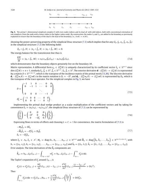
1528 M. Seslija et al. / Journal of Geometry and Physics 62 (2012) 1509–1531Fig. 5. The primal 1-dimensional simplicial complex K with even nodes indices and its dual ⋆K with odd indices, both with conventional orientation ofone simplices (from the node with a lower-index to the higher-index node). By construction, the nodes ˆv 0 and ˆv 2n are added to the boundary as previouslyexplained to insure that the boundary of the dual is the dual of the boundary, i.e., ∂(⋆K) = ⋆(∂K).showing the power-preserving property of the simplicial Dirac structure (7.3) which implies that for any (ê p , f p , e q , ˆfq , e b , ˆfb )in the simplicial structure (7.3) the following holds⟨ê p ∧ f p , K⟩ + ⟨e q ∧ ˆfq , K⟩ + ⟨e b ∧ ˆfb , ∂K⟩ = 0.The energy balance for the transmission line thus isdHdt= ⟨e b ∧ ˆfb , ∂K⟩ = e b (v 2n )ˆfb (ˆv 2n ) − e b (v 0 )ˆfb (ˆv 0 ), (7.4)which demonstrates that the boundary objects genuinely live on the boundary ∂K .Matrix representation. A differential form e q ∈ Ω 0(K) d is uniquely characterized by its coefficient vector ⃗e q ∈ R n+1 sincedim Ω 0(K) = d n+1, similarly ⃗e p, ⃗ fp ∈ R n , ⃗ fq ∈ R n+1 , ⃗e b , ⃗ fb ∈ R 2 . The exterior derivative d : Ω 0(K) → Ω 1 d d(K) is representedby a matrix D ∈ R n×(n+1) , which is the transpose of the incidence matrix of the primal mesh [13,30]. The discrete derivatived i : Ω 0(⋆ d i K) → Ω 1(⋆K) d in the matrix notation is D i = −D t , and d b : Ω 0(⋆ d b K) → Ω 1(⋆K) d is represented by D b, which isthe transpose of the trace operator. For the simplicial complex in Fig. 5, we have⎛⎞−1 1 0 · · · 0 00 −1 1 · · · 0 0D = ⎜⎝.⎟.. ⎠ ,(7.5)0 0 0 · · · −1 1 D t = −1 0 0 · · · 0 0b.0 0 0 · · · 0 1Implementing the primal–dual wedge product as a scalar multiplication of the coefficient vectors and by taking forconvenience ⃗e b = (e b (v 0 ), −e b (v 2n )) t , the simplicial Dirac structure of (7.3) can be represented by⎛ ⎞⃗ ⎛ ⎞fp 0 D 0 ⃗e p⎝ ⃗fq ⎠ = −D t 0 D b⎝⃗e q ⎠ . (7.6)⃗e b0 −D t b0 ⃗ fbExpressing flows in terms of efforts and choosing L = C = 1 for convenience, the matrix formulation of (7.3) is−M p˙⃗ep = D⃗e q− Mq˙⃗eq = −D t i ⃗e p + D b⃗ fb(7.7)⃗e b = −D t b ⃗e q,where ⃗e p ∈ Λ 0 , ⃗e q ∈ Λ 1 , M p = diag (h 1 , h 3 , . . . , h 2n−1 ) ∈ R n×n and Mq = diagĥ0 , ĥ 2 , . . . , ĥ 2n ∈ R (n+1)×(n+1) , withh 1 = |[v 0 , v 2 ]|, h 3 = |[v 2 , v 4 ]|, . . . , h 2n−1 = |[v 2n−2 , v 2n ]| and ĥ 0 = |[ˆv 0 , ˆv 1 ]|, ĥ 2 = |[ˆv 1 , ˆv 3 ]|, . . . , ĥ 2n = |[ˆv 2n−1 , ˆv 2n ]|.Error analysis. The time derivatives of the Rp ⃗ components are v2l˙⃗R p,l = h 2l−1 ė p (ˆv 2l−1 ) − ∗ė c = p h 2l−1ė p (ˆv 2l−1 ) − ė c (z)dz. p[v 2l−1 ,v 2l ]v 2l−1The Taylor’s expansion of ė c p around ˆv 2l−1 isThusė c (z) = p ėc(ˆv p 2l−1) + ∂ėc p∂z (ˆv 2l−1)(z − ˆv 2l−1 ) + ∂ 2 ė c p∂z (ˆv 2l−1) (z − ˆv 2l−1) 2+ O(z 3 ).2 2 v2lv 2l−2ė c p (z)dz = ėc p (ˆv 2l−1)h 2l−1 + 1 3∂ 2 ė c p∂z 2 (ˆv 2l−1)ĥ2l2 3+ O(h 4 2l ),