Phase diagrams of a two-dimensional Heisenberg antiferromagnet ...

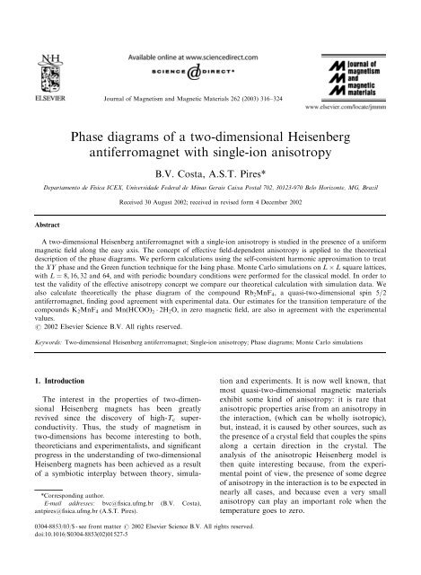
Journal of Magnetism and Magnetic Materials 262 (2003) 316–324Phase diagrams of a two-dimensional Heisenbergantiferromagnet with single-ion anisotropyB.V. Costa, A.S.T. Pires*Departamento de F!ısica ICEX, Universidade Federal de Minas Gerais Caixa Postal 702, 30123-970 Belo Horizonte, MG, BrazilReceived 30 August 2002; received in revised form 4 December 2002AbstractA two-dimensional Heisenberg antiferromagnet with a single-ion anisotropy is studied in the presence of a uniformmagnetic field along the easy axis. The concept of effective field-dependent anisotropy is applied to the theoreticaldescription of the phase diagrams. We perform calculations using the self-consistent harmonic approximation to treatthe XY phase and the Green function technique for the Ising phase. Monte Carlo simulations on L L square lattices,with L ¼ 8; 16; 32 and 64; and with periodic boundary conditions were performed for the classical model. In order totest the validity of the effective anisotropy concept we compare our theoretical calculation with simulation data. Wealso calculate theoretically the phase diagram of the compound Rb 2 MnF 4 ; a quasi-two-dimensional spin 5=2antiferromagnet, finding good agreement with experimental data. Our estimates for the transition temperature of thecompounds K 2 MnF 4 and MnðHCOOÞ 2 2H 2 O; in zero magnetic field, are also in agreement with the experimentalvalues.r 2002 Elsevier Science B.V. All rights reserved.Keywords: Two-dimensional Heisenberg antiferromagnet; Single-ion anisotropy; Phase diagrams; Monte Carlo simulations1. Introduction*Corresponding author.E-mail addresses: bvc@fisica.ufmg.br (B.V. Costa),antpires@fisica.ufmg.br (A.S.T. Pires).The interest in the properties of two-dimensionalHeisenberg magnets has been greatlyrevived since the discovery of high-T c superconductivity.Thus, the study of magnetism intwo-dimensions has become interesting to both,theoreticians and experimentalists, and significantprogress in the understanding of two-dimensionalHeisenberg magnets has been achieved as a resultof a symbiotic interplay between theory, simulationand experiments. It is now well known, thatmost quasi-two-dimensional magnetic materialsexhibit some kind of anisotropy: it is rare thatanisotropic properties arise from an anisotropy inthe interaction, (which can be wholly isotropic),but, instead, it is caused by other sources, such asthe presence of a crystal field that couples the spinsalong a certain direction in the crystal. Theanalysis of the anisotropic Heisenberg model isthen quite interesting because, from the experimentalpoint of view, the presence of some degreeof anisotropy in the interaction is to be expected innearly all cases, and because even a very smallanisotropy can play an important role when thetemperature goes to zero.0304-8853/03/$ - see front matter r 2002 Elsevier Science B.V. All rights reserved.doi:10.1016/S0304-8853(02)01527-5

B.V. Costa, A.S.T. Pires / Journal of Magnetism and Magnetic Materials 262 (2003) 316–324 317Although the quantum nature of magnetismcannot be forgotten, the study of classical modelscontinues to be an important subject of research.Field theory yields results which agree closely withexperiments on spin-1=2 Heisenberg systems butdisplay strong deviations from the predictedbehavior in systems with S > 1=2: In those systems,a broad crossover from quantum to classicalbehavior occurs at high temperatures [1]. Fromthe theoretical point of view, not everything issettled for the easy axis model. For instance, arenormalization group calculation suggests theexistence of a finite critical value of the anisotropyparameter, at which the critical temperature goesto zero [2]. However, numerical simulation andspin wave calculations do not confirm the existenceof this critical anisotropy.In this paper we will be interested in the study ofthe phase diagram of the classical anisotropicHeisenberg antiferromagnet in two dimensionsdescribed by the following Hamiltonian:H ¼ J X ~S i S ~ j D X/i;jSiSiz 2gm B H X iS z i ; ð1Þwhere the summation ð/i; jSÞ is over nearestneighbor pairs, J > 0 and the anisotropy term Destablishes an easy axis (Ising-type anisotropy). Inzero field the system undergoes a transition to atwo-dimensional magnetically ordered structure.As it is well known when a magnetic field ofsufficient strength is applied various interestingclasses of phase transitions may be induced [3].Here we consider the case of H applied along the zdirection. The low-temperature, low field orderedstate is an antiferromagnet (AF) which is separatedfrom the paramagnetic state (P) by a line ofsecond-order phase transitions. At sufficiently lowtemperature the system undergoes a first-ordertransition to a canted ‘‘spin-flop’’ state (SP) as thefield is increased. The spin-flop phase behaves likea two-dimensional XY model and thus shows nolong-range order. The state is separated from the Pphase by a second-order phase transition line. Thepoint at which AF and P phases simultaneouslybecome critical is termed the ‘‘bicritical point’’. Intwo dimensions, if a simple bicritical point occurs,it would be at T ¼ 0K:The behavior of an anisotropic Heisenbergmodel similar to Hamiltonian (1) but with anexchange anisotropy (D P i Sz i Sz j ) was first studiedby Binder and Landau [4] using Monte Carlocomputer simulations. The exchange anisotropicmodel, in zero magnetic field, has been recentlystudied by Cuccoli et al. [5] using the purequantum-self-consistent harmonic approximation.Although the qualitative features of both models,at low temperatures with single-site anisotropy orexchange anisotropy, are expected to be the same,quantitative differences do occur.In a theoretical approach, the field dependenceof Hamiltonian (1) can be taken into account as aneffective field-dependent anisotropy D eff ðHÞ [3].For a field H; applied along the easy-axis, smallerthan the spin-flop field H sf ; the effective anisotropyis given byH 2 D eff ðHÞ ¼D 1 ; ð2ÞH 2 sfwherepffiffiffiffiffiffiffiffiffiffiffiffiffiffiffiffiffiffiffiffi4JD DH sf ¼ 2S2ð3Þgm Bfor a square lattice. Clearly, while HoH sf ; theeffective anisotropy D eff is an Ising-type anisotropythat vanishes at H sf : On the other hand, as Hincreases to H > H sf ; D eff becomes negative playingthe role of a planar anisotropy which forces thespins to the lie in the XY-plane. In this XY-case,the planar behavior is enhanced as H is increasedbut this effective anisotropy approximation isvalid for fields H52H e ; where H e is the exchangefield given by H e ¼ 4JS=gm B when the system is farfrom saturation. The critical field H c ; where thesystem saturates at T ¼ 0; is given byH c ¼ 2S ð4J DÞ : ð4Þgm BIt is well known that in the classical limit,the thermodynamic properties of the antiferromagnetare the same as the ones for the ferromagnet.This allows us to do the theoreticalcalculations using a ferromagnet. Therefore, wemay now treat the system by means of the effective

318B.V. Costa, A.S.T. Pires / Journal of Magnetism and Magnetic Materials 262 (2003) 316–324HamiltonianH eff ¼J X /i;jSþ constant:~S i ~ S j D eff ðHÞ X iSiz 2ð5ÞA detailed derivation of this effective Hamiltoniancan be found in Refs. [3,6]. Of course, theconcept of an effective field-dependent anisotropycan be applied only to the classical limit (i.e. forlarge values of the spin). In fact for S ¼ 1=2 thesingle-ion anisotropy plays no role.In the usual studies of phase diagrams of 2DAF, experimental data have been qualitativelycompared with simulations [1,3]. In this work, wewill go one step further by comparing experimentaldata and simulations with theory. This paper isorganized as follows: in Section 2, we presentMonte Carlo simulations. In Section 3 we studythe Ising phase using the self consistent renormalizedspin-wave theory. The study of the XY phaseusing a self consistent harmonic approximation ispresented in Section 4. Finally in Section 5 weanalyse some previously reported experimentaldata for the compound Rb 2 MnF 4 :2. Monte CarloMonte Carlo calculations for the two-dimensionalexchange anisotropic Heisenberg modelwere performed by Binder and Landau [4]. Thoseauthors obtained the phase diagram for thatmodel, but a plot of T c as a function of theanisotropy was not presented. Also, at the timethat the work was done, the possibility of a phasetransition for the 2D isotropic Heisenberg model(as suggested by high-temperature series extrapolation)had not been completely ruled out. Later,Serena et al. [7], using Monte Carlo simulationwith an improved algorithm, obtained reliableresults for several thermodynamic properties of thesame model.Our simulations of Hamiltonian (1) were carriedout using the standard Metropolis algorithm. Wehave used lattices of size L L with L ¼8; 16; 32; 64 with periodic boundary conditions. Inorder to reach thermodynamic equilibrium, weperformed long runs of size 100 L L: In orderto extract the critical temperature T c in the Isingphase, the position of the maxima of the specificheat and magnetic susceptibility and, also, thefourth order Binder cumulant were analyzed. Toget the Berezinskii–Kosterlitz–Thouless (BKT)temperature T BKT we analyzed the helicity modulus[8]. The procedure we have adopted is asfollows: we fixed the anisotropy D while themagnetic field H was varied. For each pair ofvalues, ðH; DÞ; we then obtained the specific heat.It is known that the specific heat maximum C maxdoes not change with L in the BKT region butbehaves as C max pln L in the Ising region. Thisdistinct behavior of C max can guide us in decidingin which region, Ising or BKT we are. Then, thecorresponding critical temperature is obtained asdiscussed above. Although the model has an Isingor a BKT transition for any value of D; it is verydifficult to perform the simulation for low valuesof the anisotropy, because the critical temperaturegoes down monotonically with D; and close toT ¼ 0 the system suffers of a strong slowing down.For this reason, we have used the following valuesfor the anisotropy parameter, D=J ¼ 0:25; 0:50;1:0; 5:0 and 10:0: Our results are shown in Figs. 1,2 and 3. For all simulations, we have adoptedk B ¼ 1; J ¼ 1; S ¼ 1 , and H is in units of gm B : Wemust note that having an anisotropy parameter ofH65432100 0.5 1T cD=0.25D=0.5D=1.00Fig. 1. Phase diagramm H=JS 2 T c for some anisotropyvalues as indicated in the insert. Error bars are smaller thanthe symbols when not indicated. Lines are guide to the eyes.

B.V. Costa, A.S.T. Pires / Journal of Magnetism and Magnetic Materials 262 (2003) 316–324 319Field65432100 0.5 1TemperatureFig. 2. Phase diagramm H=JS 2 T c for D=J ¼ 1:0: Circlesand squares are simulation and theoretical results, respectively.The lines are guide to the eyes.Ln (T c/D)210-1-2-2 -1 0 1 2 3Ln (D)Fig. 3. Logarithm of T c D as a function of ln D: Circles aresimulation data and the line is the best fit.the order of the exchange constant (D=JE1) is notan unrealistic case since we have D=J ¼ 1:58 [9] forthe compound FeCl 2 :3. Ising regionThe self-consistently renormalized (SCR) spinwavetheory extends the temperature range inwhich the spin-wave theory is valid because ittakes into account the effects of dynamic interactionsbetween spin waves in the Hartee-Fockapproximation. This theory was introduced longago for the Heisenberg magnet with uniaxialanisotropy by Rastelli et al. [9] and here wereproduce their final result for the classical limit.The temperature dependent spin-wave spectrumfor Hamiltonian (5) is given byE q ðTÞ ¼4JSð1 g q Þ½1 bðTÞþZðTÞŠþ 2DS½1 2bðTÞŠ; ð6ÞwherebðTÞ ¼ T Z p Z pd~qp 2 E q ðTÞ ;ð7Þ0ZðTÞ ¼ T p 2 Z pand00Z p0g q d~qE q ðTÞ ;g q ¼ 1 2 ðcos q x þ cos q y Þ:ð8Þð9ÞEqs. (6)–(8) constitute a set of self-consistentequations for E q ðTÞ which were solved numericallyby an iterative method. These equations have asolution up to a maximum temperature T c whichwe consider to constitute the transition temperature.As can be easily seen, the SCR theorycorrectly predicts that the transition temperatureis zero when D ¼ 0: In Fig. 2, we compare ourtheoretical calculation with Monte Carlo data forD=J ¼ 1:0: Here H is in units of gm B : As we cansee, the overall agreement in the Ising region isreasonable. Then, when an uniform field, smallerthan H sf ; is applied, the Ising-like anisotropicmodel continues to provide an adequatedescription of the critical behavior. For theexchange anisotropic case with H ¼ 0 and whenD-N (or J-0), the system behaves like the pureIsing model and T c =D-1 [4]. However, forHamiltonian (1), we know that there is no phasetransition for J ¼ 0: It is therefore interesting tostudy the behavior of T c as a function of D: InFig. 3 we present our simulation data for lnðT c =DÞas a function of lnðDÞ: The data obtained can bemodelled using the following expressionln T c¼ a b lnðDÞ; ð10ÞD

320B.V. Costa, A.S.T. Pires / Journal of Magnetism and Magnetic Materials 262 (2003) 316–324with a ¼ 0:070ð12Þ and b ¼ 0:80ð10Þ: As we can seefor large values of D we have T c =DpD b quitedifferent from the exchange anisotropic case [10].Notice that we cannot obtain results using theSCR theory for the single-ion anisotropic Hamiltonian,for D-N; because this region is out of thevalidity range of the theory. However, for theexchange anisotropic case, the SCR theory givesgood agreement with classical Monte Carlosimulation for any value of the anisotropy parameter[10].4. XY regionThe two-dimensional classical model has atransition into a phase with algebraically decayingcorrelation functions and infinite susceptibility.The transition temperature, called the BKTtemperature T BKT ; can be calculated using a selfconsistentharmonic approximation [11]. In orderto properly treat the magnetic field we will firstintroduce the parametrization.~S n ¼ð 1Þ n S sin½y n þð 1Þ n y 0 Šcosf n ;sin ½y n þð 1Þ n y 0 Šsin f n ; cos½y n þð 1Þ n y 0 Š ;ð11Þwherecos y 0 ¼ H H sf: ð12ÞH c H sfInserting Eq. (12) into Hamiltonian (1) we findthat keeping only terms up to second order theHamiltonian becomesHS 2 ¼ J X4 sin2 y 0r;af r f rþa 22J X rðy r y 0 Þ 2J Xðy r y 0 Þðy rþa y 0 Þþ gm BH22r;aX cos y 0 ðy r y 0 Þ 2 : ð13ÞrRedefining the spin component Sn z bySn z ¼ S cosðy n y 0 Þ; ð14Þwe see that, from the thermodynamical pointof view, our original model is equivalent toan anisotropic ferromagnet described by theHamiltonianJ XH ¼ sin 2 y 0 Sr x 2Sx rþa þ Sy r rþa Sy þ Szr Srþaz r;aXþ D eff ðSr z Þ2 ;ð15Þr;awith D eff the effective field-dependent anisotropy.Now, in order to use the SCHA we follow thesame procedure used in Ref. [11] obtaining thequadratic form for the HamiltonianXrð1 g q Þf q f qH ¼ J 2qþ ð1g q Þþ2 D effJ Sq z Sz q ; ð16Þwhere g q is given by Eq. (9) and the stiffness r isgiven byDr ¼ sin 2 y 0 1 ðSr z 1=2 Þ2 1 ðSzrþa Þ 2 1=2E cos ðf rþa f r Þ : ð17ÞThe stiffness takes into account anharmonic termsneglected when we write the original Hamiltonianin the harmonic form. Following Ref. [11] we findthat we can write Eq. (17) asr ¼ sin 2 y 0 ½1tIðHÞŠexpwhere t ¼ T=4J; andIðHÞ ¼ 12p 2 Z p0Z p0tr; ð18Þd~q1 g q þ 2D eff =J : ð19ÞFor large fields, magnetic saturation effectsbecome important and the phase line bends backtowards the field axis intersecting it at H ¼ H c :The stiffness goes abruptly to zero at a temperatureT 0 given byT 0 ðHÞ ¼4JS 2 sin 2 y 0 e þ sin 2 1:y 0 IðHÞ ð20ÞFor small values of D eff we find4JS 2T 0 ¼lnðpJ=4D eff Þ :ð21ÞThis equation is in agreement with detailedrenormalization group calculation [12]. The stiffnesscalculated using the SCHA does not incorporatethe effect of polarization by bound vortex

B.V. Costa, A.S.T. Pires / Journal of Magnetism and Magnetic Materials 262 (2003) 316–324 321pairs. This latter mechanism is responsible for ashift in the transition temperature [13]. AtT BKTrenormalization group analysis [14] shows that thestiffness should exhibit a universal jump given by2T BKT =p: The BKT temperature for our model canthen be determined by the crossing between therðTÞ curve, calculated using Eq. (18) and the lineg ¼ 2T=p: Our calculation for the XY region isalso presented in Fig. 2. The two phase boundariesmeet at T ¼ 0 for H ¼ H sf ; with a horizontaltangent. At low temperatures, the two critical linesare so close to each other, that they cannot bedistinguished from a single spin-flop line. In theXY region, an applied field is not really equivalentto an anisotropy: increasing the field would leadthe spins to tilt out of the XY plane while a trueanisotropy would force the spins to lie in the XYplane. The SCHA works reasonably well for theanisotropic easy-plane Heisenberg model [11–15],and the effect of the tilting out of the plane wastaken into account by the sin 2 y 0 term in Eq. (18).However, even so, the quantitative agreement isgood only for the regions HBH sf and HBH c ; forother values of H; the agreement is not so good. Itseems, then, that the reduction of the spin in-planecomponent was not completely taken into accountin our calculation and a more elaborated theoryshould be developed.approximately given by [1]pH sf ¼ffiffiffiffiffiffiffiffiffiffiffiffiffiffiffiffiffiffiffiffiffiffiffiffiffiffiffiffiffi28:09 þ 0:23T; ð22Þwhere T is the temperature in Kelvin, and H isgiven in Tesla. For a 2D system, described byHamiltonian (1), we would have just a bicriticalpoint at T ¼ 0: A line of zero anisotropy impliesthe existence of long range order for H ¼ H sf : Thecomparison of our theoretical calculation with theexperiments of Ref. [1] is shown in Figs. 4 and 5.Aquantum SCHA for an easy-plane model with S ¼5=2 gives results similar to the ones using theclassical approximation [18] and, therefore, in theXY region we are allowed to use the simplerclassical approach presented in Section 4. Thehigher-field phase boundary can be fitted reasonablywell by our theory. In Fig. 4 we use the valueD ¼ 0:148 K; and in Fig. 5 we use a temperaturedependent value obtained using Eq. (22). For H7655. Rb 2 MnF 4A material which is particularly close to classicaltwo-dimensional models seems to be Rb 2 MnF 4which has spin S ¼ 5=2 [16]. At zero field thiscompound is a weakly Ising antiferromagnet withJ ¼ 7:31 K: The principal spin anisotropy is anuniaxial magnetic interaction with gm B H A ¼0:371 K evaluated at a temperature of T ¼ 4:2K;along the z-axis perpendicular to the magneticplane. Using the relationDS 2 ¼ gm B H A S;we find D ¼ 0:148 K: The magnetic ordering hasbeen described by Birgeneau et al. [17]. In zerofield, the system undergoes a transition to a 2Dmagnetically ordered structure at 38:4K: The lineof zero anisotropy was experimentally found to beField (T)432100 10 20 30 40Temperature (K)Fig. 4. Phase diagram for Rb 2 MnF 4 in an external magneticfield perpendicular to the magnetic planes. The experimentaldata (circles) are from Ref. [1]. Squares represent Greenfunction calculation in the Ising region and SCHA in the XYregion. Diamonds are the SCR calculation.

322B.V. Costa, A.S.T. Pires / Journal of Magnetism and Magnetic Materials 262 (2003) 316–324Field (T)7654This technique has been used by Dalton and Wood[20] and Reinehr Figueiredo [21] to study theferromagnet with exchange anisotropy. The retardedGreen function for Heisenberg operators Aand B is defined asG A;B ðtÞ iyðtÞ/½AðtÞ; Bð0ÞŠS; ð23Þin which yðtÞ is the step function equal to 1 fort > 0; 0 for to0: The equation of motion for thetime-Fourier transformation of G AB ðtÞ given by0A; BT ¼ 1 Z þNG AB ðtÞe iot dt;2pisNo0A; BT ¼ 12p /½A; BŠS þ 0½AðtÞ; HŠ; Bð0ÞT; ð24Þ30 10 20 30 40Temperature (K)where H is the Hamiltonian of the system. ForHamiltonian (1) we findFig. 5. Phase diagram for Rb 2 MnF 4 in an external magneticfield perpendicular to the magnetic planes.The experimentaldata (circles) are from Ref. [1]. Squares are Green functioncalculations taking into account the interplanar coupling.Diamonds are Green function calculations in the Ising regionand SCHA in the XY region, with a temperature dependentanisotropy.o0Sn þ ; S m T ¼ 1 p /Sz n Sd m;nþ J X 0S þ nþd Sz n ; S m Td0Sn z Sþ nþd ; S m T0Snþd z Sþ n ; S mTþ D eff 0Sn þ Sz n ; S m Tþ 0Sn z Sþ n ; S m T :ð25Þup to 7 T, the effective anisotropy formulation isexpected to work since, in this case, H c E65 T: Inthe Ising phase, for a more precise comparisonwith the experimental data, we performed aquantum SCR calculation. We obtain the quantumSCR expression by replacing T=E q byðexpðE q =TÞ 1Þ 1 in Eqs. (7) and (8) [9]. However,now, due to the exponential term, the numericalsolution of the self consistent equations must beperformed in a very carefull way since the accuracydecreases with decreasing temperature. In Fig. 4we also show the theoretical calculation using theSCR technique. The results are not very differentfrom the ones obtained using the Green functiontechnique described below which is a moreconvenient approach and easier to calculate [19].In order to solve Eq. (25) we use the random-phaseapproximation to decouple the higher order Greenfunction, this is0S z n Sþ m ; S j T ¼ /S z n S0Sþ m ; S j T;to obtaino0S þ n ; S m T¼ 1 p /Sz n Sd m;n þ 2J/Sn z S X 0S þ nþd ; S m T þ 0Sþ n ; S m Tdþ 2D eff /S z n S0Sþ n ; S m T:ð26Þð27ÞWe remark that in the limit J-0 (and H ¼ 0) wehave /S z S-0 even if Da0; and the above

B.V. Costa, A.S.T. Pires / Journal of Magnetism and Magnetic Materials 262 (2003) 316–324 323procedure does not work. Making use of thetranslational invariance of the system we maydefine the Fourier transformsGðq; oÞ ¼ X m;n0S þ n ; S m Teiqðn mÞ ; ð28Þin terms of which Eq. (27) becomesGðq; oÞ ¼ /Sz S 1p o oðqÞ ; ð29ÞwhereoðqÞ ¼8/S z S½Jð1 g q ÞþD eff Š; ð30Þis the magnon energy spectrum and g q was definedin (9). Using the relation/ABS ¼ lime-0iZ þNNGðo þ ieÞ Gðo ieÞdo;expðboðqÞÞ 1ð31Þwe find the following expression for the magnetization:1/S z S ¼ S Z ð2pÞ 2 coth boðqÞ dq 2 :ð32Þ2Near the critical temperature, where /S z S goes tozero, we can expand the argument in the integraland obtain1¼ 1 Z1 d 2 qT c 4S 2p 2 : ð33ÞJð1 g q ÞþD effPerforming the integral in the q y variable, we find1¼ 1 Z1 pdq xq ffiffiffiffiffiffiffiffiffiffiffiffiffiffiffiffiffiffiffiffiffiffiffiffiffiffiffiffiffiffiffiffiffiffiffiffiffiffiffiffiffiffiT c 4JS 2p 2 ; ð34Þ0ð2 þ B cosq x Þ 2 1where B ¼ 2D eff =J: For B small we can solve theintegral analytically and obtain1¼ 1 T c 4JSp ln p : ð35ÞBBefore interpreting the data for Rb 2 MnF 4 let usapply Eq. (34) to two other compounds [22]. ForK 2 MnF 4 we have J ¼ 8:4K; D ¼ 0:134 K whichleads to T c ¼ 42:73 K: The experimental value is42:3K: The second compound is MnðHCOOÞ 2 2H 2 O: We have J ¼ 0:70 K; D ¼ 0:0114 K: Wefind T c ¼ 3:57 K; to be compared with the experimentalvalue 3.68 K. Just for comparison, thequantum SCR gives T c ¼ 42:19 K and T c ¼ 4:09 Krespectively. For Rb 2 MnF 4 ; if we take D temperaturedependent, using for D the effective anisotropydefined in Eq. (2) with H sf given by Eq. (22)and calculate T c using Eq. (34) we obtain T c ¼40:53 K: Otherwise using the temperature independentvalue for the anisotropy, D ¼ 0:148 K; wefind T c ¼ 38:73 K; to be compared with theexperimental value 38:4K:In the Ising region are seen deviations from thecalculations. This can be attributed to the destructionof the pure planar anisotropy in the high fieldphase. The 2D XYphase is extremely sensitive tosymmetry breaking interactions and to the interplanarcoupling. Any of these effects move thebicritical point from T ¼ 0 to a non-zero temperature.The interplanar coupling is often sosmall that the observed transition is primarilyinduced by anisotropy. The experimental data areconsistent with a BCP at a temperature near 30 K.Let us consider an orthorhombic anisotropy:this would correspond to Hamiltonian (1) with anadditional small anisotropy term D x ðSn xÞ2 : ForHoH sf the effective anisotropy is of the Ising-typeand the behavior is comparable to the uniaxialcase. Let us take H ¼ H eff ; use the experimentalvalue T c ¼ 30 K and determine the value of theparameter D x : For a positive D x a Kosterlitz–Thouless transition should occur at the bicriticalpoint T bc ¼ 30 K if D x ¼ 0:0212 K: Otherwise anegative term would lead to an order–disorder(Ising) transition with D x ¼ 0:028 K: An interplanarcoupling J 0 ; treated by the Green functionmethod, would have to have the value a ¼ J 0 =J ¼0:01; to give T bc ¼ 30 K; a value too high since it isexpected that a should be around 10 6 : We remarkthat this last value of a leads to T bc ¼ 12:5K: Thedashed line in Fig. 5 describes the result consideringinterplanar coupling with a ¼ 0:01: A similarcurve would be obtained in the case of anorthorhombic anisotropy. Here we have used thevalues of J and D given in Ref. [1]. Theexperimental data of those authors differ slightlyfrom the ones obtained by Cowley et al. [16]. Ofcourse we could vary D and D x to get a better fit to

324B.V. Costa, A.S.T. Pires / Journal of Magnetism and Magnetic Materials 262 (2003) 316–324experimental data. However, considering theapproximate nature of the theories we have used,and the precision of the experimental data we donot see a valid reason for doing so. We concludethat it is not yet completely clear what themechanism is which is responsible for the bicriticalpoint in Rb 2 MnF 4 : More detailed experiments areneeded to elucidate this point.AcknowledgementsThis work was partially supported by CNPq andFAPEMIG (Brazilian agencies). Numerical workwas done in the LINUX parallel cluster at theLaborat !orio de Simula-c *ao Departamento de F!ısica- UFMG.References[1] R.J. Christianson, R.L. Leheny, R.J. Birgeneau, R.W.Erwin, Phys. Rev. B 63 (2001) 140401;R.L. Leheny, R.L. Christianson, R.J. Birgeneau, R.W.Erwin, Phys. Rev. Lett. 82 (1999) 418.[2] N.S. Branco and J. Ricardo de Sousa, cond-mat/0006345(June 2000).[3] H.J.M. De Groot, L.J. De Jongh, Physica B 141 (1986) 1.[4] K. Binder, D.P. Landau, Phys. Rev. B 13 (1976) 1140;D.P. Landau, K. Binder, Phys. Rev. B 24 (1981) 1391.[5] A. Cuccoli, T. Roscilde, V. Tognetti, R. Vaia, P. Verruchi,Eur. Phys. J. B 20 (2001) 55.[6] A.S.T. Pires, M.E. Gouv#ea, J. Phys. C 17 (1984) 4009.[7] P.A. Serena, N. Garcia, A. Levanyuk, Phys. Rev. B 47(1993) 5027.[8] B.V. Costa, A.S.T. Pires, Phys. Rev. B.[9] E. Rastelli, A. Tassi, L. Reatto, J. Phys. C 7 (1974)1735.[10] M.E. Gouv#ea, G.M. Wyzin, S.A. Leonel, A.S.T. Pires,T. Kampeter, F.G. Mertens, Phys. Rev. B 59 (1999) 6229.[11] S.L. Menezes, M.E. Gouvea, A.S.T. Pires, Phys. Lett. A166 (1992) 330.[12] D. Fisher, Phys. Rev. B 39 (1989) 11783.[13] P. Minnhagen, Rev. Mod. Phys. 59 (1987) 1001.[14] D.R. Nelson, J.M. Kosterlitz, Phys. Rev. Lett. 39 (1977)1201.[15] A.S.T. Pires, Phys. Rev. B 54 (1996) 6081.[16] R.A. Cowley, A. Aharony, R.J. Birgeneau, R.A. Pelcovits,G. Shirane, T.R. Thurston, Z. Phys. B 93 (1993) 5;R.A. Cowley, G. Shirane, R.J. Birgeneau, H.J. Guggenheim,Phys. Rev. B 15 (1977) 4292.[17] R.J. Birgeneau, H.J. Guggenheim, G. Shirane, Phys. Rev.B 8 (1970) 2211.[18] A.S.T. Pires, Phys. Rev. B 53 (1996) 235.[19] S.V. Tyablikov, Methods in the Quantum Theory ofMagnetism, Plenum, New York, 1967.[20] N.W. Dalton, D.W. Wood, Proc. Phys. Soc. 90 (1967) 459.[21] E.E. Reinehr, W. Figueiredo, Phys. Rev. B 52 (1995) 310.[22] L.J. De Jongh, L.P. Regnault, J. Rossat-Mignod, J.Y.Henry, J. Appl. Phys. 53 (1982) 7963.