Coupling 1D and 2D elasticity problems by using the hp-d-version of ...

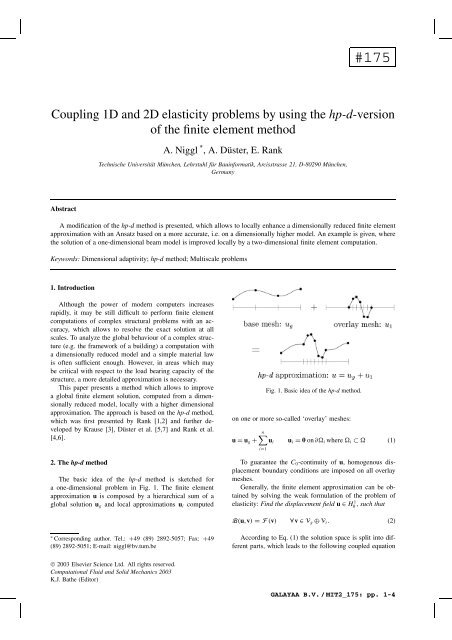
#175Coupling 1D and 2D elasticity problems by using the hp-d-versionof the finite element methodA. Niggl * ,A.Düster,E.RankTechnische Universität München, Lehrstuhl für Bauinformatik, Arcisstrasse 21, D-80290 München,GermanyAbstractA modification of the hp-d method is presented, which allows to locally enhance a dimensionally reduced finite elementapproximation with an Ansatz based on a more accurate, i.e. on a dimensionally higher model. An example is given, wherethe solution of a one-dimensional beam model is improved locally by a two-dimensional finite element computation.Keywords: Dimensional adaptivity; hp-d method; Multiscale problems1. IntroductionAlthough the power of modern computers increasesrapidly, it may be still difficult to perform finite elementcomputations of complex structural problems with an accuracy,which allows to resolve the exact solution at allscales. To analyze the global behaviour of a complex structure(e.g. the framework of a building) a computation witha dimensionally reduced model and a simple material lawis often sufficient enough. However, in areas which maybe critical with respect to the load bearing capacity of thestructure, a more detailed approximation is necessary.This paper presents a method which allows to improvea global finite element solution, computed from a dimensionallyreduced model, locally with a higher dimensionalapproximation. The approach is based on the hp-d method,which was first presented by Rank [1,2] and further developedby Krause [3], Düster et al. [5,7] and Rank et al.[4,6].2. The hp-d methodThe basic idea of the hp-d method is sketched fora one-dimensional problem in Fig. 1. The finite elementapproximation u is composed by a hierarchical sum of aglobal solution u g and local approximations u i computedFig. 1. Basic idea of the hp-d method.on one or more so-called ‘overlay’ meshes:u = u g +n∑u i u i = 0 on∂ i where i ⊂ (1)i=1To guarantee the C 0 -continuity of u, homogenous displacementboundary conditions are imposed on all overlaymeshes.Generally, the finite element approximation can be obtainedby solving the weak formulation of the problem ofelasticity: Find the displacement field u ∈ H0 1 , such thatB(u,v) = F (v) ∀v ∈ V g ⊕ V i . (2)∗ Corresponding author. Tel.: +49 (89) 2892-5057; Fax: +49(89) 2892-5051; E-mail: niggl@bv.tum.beAccording to Eq. (1) the solution space is split into differentparts, which leads to the following coupled equation© 2003 Elsevier Science Ltd. All rights reserved.Computational Fluid and Solid Mechanics 2003K.J. Bathe (Editor)GALAYAA B.V. / MIT2_175: pp. 1-4

2 A. Niggl et al. / Second MIT Conference on Computational Fluid and Solid Mechanicssystem (only one overlay mesh is assumed):B(u g + u 1 ,v g ) = F (v g ) ∀v g ∈ V g(3)B(u g + u 1 ,v 1 ) = F (v 1 ) ∀v 1 ∈ V 1Due to its linearity, we can split the bilinear form B(·,·)and bring the mixed terms to the right hand side. Theresulting equation system can then be solved by applying ablock Gauss–Seidel iteration:B(u (k+1)g,v g ) = F (v g ) − B(u (k)1 ,v g)B(u (k+1)1,v 1 ) = F (v 1 ) − B(u (k+1)g,v 1 )The mixed terms in Eq. (4), e.g.∫B(u (k)1 ,v g) = ε(v g ):σ(u (k)1 )d= 1 ∩ g∫ 1 ∩ g(4)ε(v g ):C : ε(u (k)1)d (5)can be interpreted as an additional negative load vectorresulting from the stresses σ(u (k)1 )orthestrainsε(u(k) 1 )ofthe previous iteration step. The advantage of this approachis that no complicated quadrature scheme has to be appliedto compute the coupled stiffness matrix explicitly. Wetherefore only have to transfer the results from one mesh tothe other one and apply them as prestresses (or prestrains)to the actual iteration step.3. Coupling 1D and 2D problemsGenerally, there is no reason that the different termsin Eq. (1) have to be computed with the same method.Therefore one can choose the global approximation u g ,such that it allows a cheap analysis, based, for example,on a dimensionally reduced model, which represents theglobal behaviour of the structure accurately enough. Onlyin areas, where the model error exceeds a certain limit,the solution is extended locally by a higher dimensionalAnsatz.In this paper, the global approximation u 1Dgis computedfrom a one-dimensional beam model. In the caseof uniaxial bending, the solution is given by the three independentvariables u(x),w(x),(x), i.e. the longitudinaldisplacement, the deflection and the rotation, respectively.In areas where a critical model error is to be expected,a two-dimensional mesh is defined locally. The 1D solutionis extended via the kinematic model assumptions to thetwo-dimensional case and applied to all integration pointsof the overlay mesh:( )( )u 2Dg (x, y) = ux (x, y) −(x)y + u(x)(6)u y (x) w(x)From this displacement field the strainsε(u 2Dg ): ε x = ∂u x∂x , ε y = 0, γ = ∂u x∂y + ∂u y(7)∂xare computed, acting as negative loads to the second part ofEq. (4)∫B(u 1 ,v 1 ) = F (v 1 ) − ε(v 1 ):C : ε(u 2Dg). (8) 1Solving this equation system, we obtain the approximationu 2D1on the overlay mesh, which is added to u 2Dg .Generally, the overlay solution u 2D1must be projected to thedimensionally reduced model in order to calculate the nextiteration step, see Eq. (4). However, numerical tests haveshown that this iteration is often not necessary in practice.Only one iteration step is needed to obtain an accurateextension to the dimensionally reduced, global solution.4. Numerical exampleIn the following example we consider a linear elasticbeam with two holes. The beam of length l, thicknessb and height h is clamped at both ends and loaded byan uniform pressure p = 1MN/m 2 . Figure 2 shows theone-dimensional model of the structure.Assuming the Bernoulli theory for beam bending, ananalytical solution for the deflection w(x) and the rotation(x) can be given byw(x) = 124EI pl2 x 2 − 112EI plx3 + 124EI px4 ,(x) = ∂w∂x , (9)where E denotes Young’s modulus and I = bh 3 /12 representsthe moment of inertia. The procedure to improvethe 1D solution in the vicinity of the left hole is sketchedin Fig. 3. The first mesh shows the stress σ x of the 1DFig. 2. One dimensional model of the beam with two holes.GALAYAA B.V. / MIT2_175: pp. 1-4

A. Niggl et al. / Second MIT Conference on Computational Fluid and Solid Mechanics 3Fig. 3. Improvement of the dimensionally reduced approximation in the vicinity of the left hole.beam solution in Eq. (9), extended to the two-dimensionalcase. Based on this solution, u 1 is computed on the overlaymesh according to Eq. (8). Finally, the composed solutionσ x (u) = σ x (u g ) + σ x (u 1 ) is shown at the bottom of theFig. 3.The same approach can be used to ‘plaster’ incompatiblefinite element meshes of n local sub-models. Then Eq. (4)reads:∑B(u 1 ,v 1 ) = F (v 1 ) − B(u g ,v 1 ) − n B(u j ,v 1 )j≠1...∑B(u i ,v i ) = F (v i ) − B(u g ,v i ) − n B(u j ,v i )j≠i(10)Each single overlay problem can be computed therebycompletely independently.Figure 4 illustrates this technique for the previouslypresented example. The solution at the hole on the righthand side of the beam is computed on a different mesh. Itis not necessary that the two overlay meshes must coincideon their boundaries, they even can be overlapping.5. ConclusionsThe method presented in this paper allows a computationallycheap ‘level-of-detail’ analysis using a hierarchy ofmodels. Considering more complex structural problems, itallows to analyze special details of the structure independently,based on a global ‘background’ solution only. Thesame technique can be used to couple higher dimensionalFig. 4. Improvement of the 1D beam approximation by two independent overlay solutions, stresses σ x is plotted.GALAYAA B.V. / MIT2_175: pp. 1-4

4 A. Niggl et al. / Second MIT Conference on Computational Fluid and Solid Mechanicsmodels or to apply different material models on each levelof detail.Finally, an improvement of the method could beachieved by applying an a-posteriori error estimator whichhelps to detect the model error of the lower dimensionalapproximation. This would allow for an adaptive solutionscheme, which automatically enhances the solution in areas,where a significant model error occurs.References[1] Rank E. Adaptive remeshing and hp domain decomposition.Computer Methods in Applied Mechanics and Engineering1992; 101:299–313.[2] Rank E. A combination of hp-version finite elements and adomain decomposition method. In Proceedings of the FirstEuropean Conference on Numerical Methods in Engineering,Brüssel, 1992.[3] Krause R. Multiscale computations with a combined h-and p-version of the finite-element method. PhD Thesis,Fach Numerische Methoden und Informationsverarbeitung,Universität Dortmund, 1996.[4] Rank E, Krause R. A multiscale finite-element-method.Comput Struct 1997;64:139–144.[5] Düster A, Rank E, Steinl G, Wunderlich W. A combinationof an h- andp-version of the finite element methodfor elastic-plastic problems. In: Proceedings of ECCM ’99,European Conference on Computational Mechanics 1999,München.[6] Rank E, Düster A. Dimensional adaptivity using the p-version of the finite element method. In: Proceedings of theEuropean Conference on Computational Mechanics 2001,Cracow 2001.[7] Düster A. High order finite elements for three-dimensional,thin-walled nonlinear continua. PhD Thesis, Lehrstuhl fürBauinformatik, Technische Universität München, 2001.GALAYAA B.V. / MIT2_175: pp. 1-4