Simulating a Simple Real Business Cycle Model using Excel

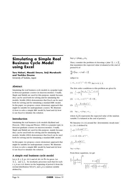
Simulating a Simple RealBusiness Cycle Modelusing ExcelToru Hokari, Masaki Iimura, Seiji Murakoshiand Yoshiko OnumaUniversity of Tsukuba, JapanAbstractSimulating the real business cycle models is a popular topicin first-year graduate courses on macroeconomics. Usually,Maple and Matlab are used for this purpose, mainly becausethey can be used both for solving and for simulating themodels. Strulik (2004) demonstrates that Excel can be usedboth for solving and for simulating a standard RBC model.In this paper, we propose a more elementary approach thatmight be suitable for undergraduate courses. We illustrate(i) how to solve a simple RBC model by hand and (ii) howto use Excel to simulate the solution.IntroductionSimulating the real business cycle models (Kydland andPrescott, 1982; Long and Plosser, 1983) is a popular topic infirst-year graduate courses on macroeconomics. Usually,Maple and Matlab are used for this purpose, mainly becausethey can be used both for solving and for simulating themodels. Strulik (2004) demonstrates that Excel can be usedboth for solving and for simulating a standard RBC model.In this paper, we propose a more elementary approach thatmight be suitable for undergraduate courses. We illustrate(i) how to solve a simple RBC model by hand and (ii) howto use Excel to simulate the solution.A simple real business cycle modelLet α, β, γ, δ, ρ∈ (0,1) and z0, k0, σ∈R+ be given. Let{} ε∞ and {} ∞ t t =1zt t =1be stochastic processes such that for eacht, ε t is an i.i.d. drawn (at the beginning of period t) from thenormal distribution N(0,σ 2 ), and z t is a random variabledefined bylog z t = ρlogz t–1 +ε t .Then, consider the problem of choosing a ‘plan’ {( c )} ∞ t, lt, ktt=0that maximises the expected value (evaluated at the end ofperiod 0) of∑ ∞t=0subject toc + ktβfor t = 0, 1, 2,The first order conditions to this problem are given byα −11−α1 ⎡αz+ − ⎤t+1kt+ 1lt+11 δ(1) = βEt⎢⎥,ct⎢⎣ct+ 1 ⎥⎦α 1−α(2) c t+ k t= z tk tl t+ ( − δ ) k t ,α −αγ ( 1−α)ztktlt(3) =,1−l c(4) log zt+ 1= ρ log z t+ εt+1 .where E t [X] represents the expected value of the randomvariable X evaluated at the end of period t.We linearise (1)–(4) around the ‘deterministic steady-state’(c, l, k, z) defined by1 1−δ + αzk= β ⋅ccα 1−αc + k = ( 1−δ ) k + zk l ,γ=1−l[ log c + γ log( 1−l )]tα 1−αt + 1≤ z tk tl t+ 1( 1−α)αzk lclog z = ρ log z .tt+ 11−αFrom these equations, we get1( − δ ) k tlα −11−α,tt,⎛ ⎞1−α⎜ ⎟k αα= ⎜ ⎟⎛ k ⎞l ⎜ 1 ⎟(1 − α)⎜ ⎟⎜ −1+δ ⎟ ,⎝ l ⎠⎝ β ⎠ l =αα⎛⎞⎜⎛k ⎞ ⎛ k ⎞ ⎛ ⎞− δ ⎟kγ + −α⎜ ⎟ ⎜ ⎟ (1 )⎜ ⎟ ,⎝⎝l ⎠ ⎝ l ⎠⎠⎝ l ⎠Page 16 CHEER Volume 19

⎡ q22−11Q =⎢− qq⎢11q22− q12q21⎢⎣0and⎡λ10 0 ⎤⎢−1M0= Q 0 λ20⎥Q⎢ ⎥⎢⎣0 0 λ ⎥3 ⎦.⎤⎥⎥⎥⎦,By pre-multiplying both sides of (10) by Q –1 , and by putting1⎡x⎤t ⎡cˆt ⎤⎢ 2 ⎥ −1≡⎢ ⎥ ,⎢xt⎥ Q kˆ⎢t⎥⎢3⎥⎣x⎦⎢⎣⎥tzˆt ⎦we obtain1⎡x⎤t ⎡λ10⎢ 2 ⎥=⎢⎢xt⎥ 0 λ⎢2⎢3⎥⎣x⎦⎢t ⎣ 0 0Taking the expected value of both sides evaluated at theend of period t,1⎡x⎤t ⎡λ1⎢ 2 ⎥=⎢⎢xt⎥ 0⎢⎢3⎥⎣x⎦⎢t ⎣ 0It follows that for each T>0,shown that ⎢λ 1 ⎢

zˆ= ρzˆ+ zε,101ˆˆ a ˆ21c0+ a22k0+ a23zˆ0k1=,b22enter=$B$7*C30+$D$7*B31|in cell C31, and=($B$17*G30+$B$18*D30+$B$19*C30)/$B$20in cell D31.Step 8. Copy the cells A31–F31 into subsequent rows. Thenwe obtain a simulated time series of z 1 , ˆk 1 , ĉ 1 , and ˆl 1 .Figure 3Figure 4Figure 5Leti ≡ ktt+1y ≡ c + i ,t− (1 − δ ) k ,i ≡ k − (1 − δ ) k = δk,y ≡ c + k − (1 − δ ) k = c + δk,y ˆ ˆˆt− y cct+ kkt+1− (1 − δ ) kktyˆt≡ =,yyˆ (1 ) ˆˆit− i kkt+ 1− − δ kktit≡ =,iiα −11−α( ˆ )( ˆ α −1) ( ˆ 1−αrt≡ αztktlt− δ = α zzt+ z kkt+ k llt+ l)− δ ,α −αw ≡ (1 − ) z k l = (1 − )( zzˆ+ z)(kkˆα+ k)( llˆ−ααα+ l),tttttttα −αw ≡ (1 − α)zk l ,(1 )( zzˆz)(kkˆαw wk)( llˆ−t− −αt+t+t+ l)wˆt≡ =wwt− w.By considering these variables together with z 1 , ˆk 1 , ĉ 1 , andˆl 1 , one can create a table and a figure (Figures 6 and 7)similar to Table 3 and Figure 10 of King and Rebelo (1999). 1tαtFigure 6CHEER Volume 19 Page 19

Notes1 Sample Excel files are available athttp://member.social.tsukuba.ac.jp/hokari/ReferencesFarmer, R.E.A. (1999) Macroeconomics of Self-fulfillingProphecies,2nd ed, MIT Press.King, R.G., and S.T. Rebelo (1999) ‘Resuscitating real businesscycles’ in Handbook of Macroeconomics, volume 1B, by J.B.Taylor and M. Woodford (Eds), Elsevier, 927–1007.Kydland, F. and E. Prescott (1982) ‘Time to build and aggregatefluctuations’, Econometrica 50, 1345–1371.Long, Jr., J.B. and C.I. Plosser (1983) ‘Real business cycles’,Journal of Political Economy 91, 39–69.Strulik, H. (2004) ‘Solving rational expectations models usingExcel’, Journal of Economic Education 35, 269–283.Contact detailsToru HokariAssociate ProfessorGraduate School of Humanities and Social SciencesUniversity of TsukubaFigure 71-1-1 Ten’nodaiTsukubaIbaraki, 305-8571JapanEmail: hokari@social.tsukuba.ac.jpFax: +81-298-53-6611Page 20 CHEER Volume 19