Variational Principles in Conformation Dynamics - FU Berlin, FB MI

More documents

Recommendations

Info

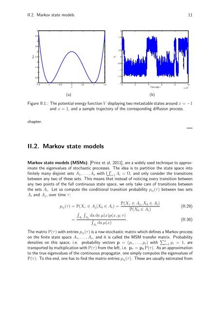
10 II. The variational principleThe spectral decomposition, the Chapman-Kolmogorov equation Lemma II.1 and the assumptionP(τ)φ → φ for all φ ∈ L 2 µ −1 (Ω) show us that the i-th eigenvalue λ i (τ) is acontinuous function of τ and satisfies λ i (τ 1 +τ 2 )=λ i (τ 1 )λ i (τ 2 ) as well as λ i (0) = 1. Therefore,it can be written as λ i (τ) =e −κ iτ for some κ i > 0, thatis,ithasanexponentialdecayrate. Clearly, κ 1 =0and κ 2 ,...,κ m are close to zero. Looking at the action of P(τ) onsome function ρ once more shows thatP(τ)ρ =∞ρ | φ i µ −1 P(τ)φ i =i=1∞e −κiτ ρ | φ i µ −1 φ i .i=1(II.27)If the time lag τ is very close to zero, almost all terms in the above sum will contribute. Ifτ becomes larger, however, there is a range of time lags τ where, for i>m,allexponentialdecay terms e −κiτ have essentially vanished, whereas all terms with i ≤ m still contribute. Ifτ increases even further, namely if τ 1 κ 2,therearenocontributionsexcepttheveryfirstterm. For a probability distribution ρ, wehaveρ | φ 1 µ −1 = ρ | µ µ −1 =1,soP(τ)ρ ≈ µ.The system is then distributed according to its equilibrium distribution and has basically“forgotten“ the initial deviation from equilibrium expressed by ρ. Eachdominanteigenvaluedefines a time scale 1 κ iand a corresponding slow process which equilibrates only if one waitsmuch longer than this time scale. The slow processes are the link between eigenvalues andmetastable states. A slow process usually corresponds to an equilibration process between twometastable regions, and the implied time scale 1 κ i= − τlog λ idefines an average transition(τ)time. For this reason, the approximation of dominant eigenvalues is of such importance.Example 2: Consider a four state system with stochastic transition matrix⎛⎞0.7571 0.2429 0 0P= ⎜ 0.1609 0.8306 0.0085 0⎟⎝ 0 0.0084 0.8294 0.1622 ⎠ .0 0 0.2413 0.7587(II.28)Clealy, most of the transitions will occur either between states x 1 and x 2 or between x 3 andx 4 ,whereasatransitionfromx 2 to x 3 will be a very rare event. Grouped together, x 1 , x 2 andx 3 , x 4 form two metastable states. The eigenvalues are λ 1 =1, λ 2 =0.9900, λ 3 =0.5964and λ 4 =0.5894. Clearly, there is one dominant eigenvalue related to the slow transitionprocess between the two metastable states.Example 3: In chapter 2, we will discuss the diffusion process of a one-dimensional particlein an energy landscape V .TheparticleissubjecttoaforceF ,whichequalsthederivativeofthe energy function, but is additionally perturbed by random fluctuations. For the potentialfunction V shown in Figure II.1a, theparticlewillspendmostofthetimearoundoneofthetwo minima of V ,andwilljustoccasionallycrossthebarrierseparatingthem. Figure II.1bshows a trajectory of the process, where the metastable behaviour is clearly visible. This isanother typical example of metastable states, we will investigate it in more detail in the next
II.2. Markov state models 11524.51.543.5130.5V(x)2.5X t02−0.51.51−10.5−1.50−1.5 −1 −0.5 0 0.5 1 1.5x−20 2 4 6 8 10Time step tx 10 4(a)(b)Figure II.1.: The potential energy function V displaying two metastable states around x = −1and x =1,andasampletrajectoryofthecorrespondingdiffusionprocess.chapter.II.2. Markov state modelsMarkov state models (MSMs), [Prinz et al, 2011], are a widely used technique to approximatethe eigenvalues of stochastic processes. The idea is to partition the state space intofinitely many disjoint sets A 1 ,...,A s with si=1 A i =Ω,andonlyconsiderthetransitionsbetween any two of these sets. This means that instead of noticing every transition betweenany two points of the full continuous state space, we only take care of transitions betweenthe sets A i . Let us compute the conditional transition probability p ij (τ) between two setsA i and A j ,overtimeτ:p ij (τ) =P(X τ ∈ A j |X 0 ∈ A i )= P(X τ ∈ A j ,X 0 ∈ A i )P(X 0 ∈ A i )=A i(II.29)A jdx dy µ(x)p(x, y; τ). (II.30)A idx µ(x)The matrix P(τ) with entries p ij (τ) is a row-stochastic matrix which defines a Markov processon the finite state space A 1 ,...,A s ,anditiscalledtheMSMtransfermatrix. Probabilitydensities on this space, i.e. probability vectors p =(p 1 ,...,p s ) with si=1 p i =1,aretransported by multiplication with P(τ) from the left, i.e. p τ = p 0 P(τ). As an approximationto the true eigenvalues of the continuous propagator, one simply computes the eigenvalues ofP(τ). Tothisend,onehastofindthematrixentriesp ij (τ). Theseareusuallyestimatedfrom
Page 1: Freie Universität BerlinInstitut f
Page 5: Table of contentsI. Introduction 3I
Page 8 and 9: 4 I. IntroductionFigure I.1.: An in
Page 10 and 11: 6 II. The variational principlerega
Page 12 and 13: 8 II. The variational principleIn E
Page 16 and 17: 12 II. The variational principlesim
Page 18 and 19: 14 II. The variational principleFor
Page 20 and 21: 16 II. The variational principleSin
Page 22 and 23: 18 II. The variational principleThe
Page 25 and 26: III.Diffusion processes andapplicat
Page 27 and 28: III.2. Diffusion process 23time ∆
Page 29 and 30: III.3. Numerical considerations 25W
Page 31 and 32: III.4. Diffusion in a quadratic pot
Page 33 and 34: III.5. Two-well potential 29molecul
Page 35 and 36: IV.Application to moleculesIn this
Page 37 and 38: IV.1. The example system 33221.81.8
Page 39 and 40: IV.2. Simulation 35Quantity Symbol
Page 41 and 42: IV.3. Application of the Roothan-Ha
Page 47 and 48: V. Summary and outlookWe have prese
Page 49 and 50: A. AppendixA.1. Diffusion in a quad
Page 51 and 52: A.1. Diffusion in a quadratic poten
Page 53: A.1. Diffusion in a quadratic poten
Page 57 and 58: Bibliography[Behrends, 2011] Ehrhar

Variational Principles in Conformation Dynamics - FU Berlin, FB MI

Create successful ePaper yourself

Delete template?

Save as template?