An exact method for computing the area moments of ... - IEEE Xplore

More documents

Recommendations

Info

636 IEEE TRANSACTIONS ON PATTERN ANALYSIS AND MACHINE INTELLIGENCE, VOL. 23, NO. 6, JUNE 2001Z 1Substituting for ' 0 p …t† from (6), we get Both these properties together imply 2……m ‡ n ‡ 1†!†relations, which are used to accelerate the computationFor the example given in Fig. 1, we haveI m;n ˆ 1 XXc k c ‰mŠ ‰n‡1Ši d j ' p …t i 1 † ...g 0 …l† ˆ 0 1 n ‡ 1…l ‡ 2† ˆ… 2 k2R i2R m‡11…25†j2R†…l ‡ 2†g 0 : …0:5; 0; 0:5†; l 2f1; 0; 1g;' p …t i m †' p …t j 1 † ...' p …t j n‡1 †' 0 …t k†dt:where n is the causal B-spline function of degree n. The integral in the above equation is equivalent toRNow, for the polygon, c…k† : …1; 1; 6; 8; 7; 4† and d…k† :11 '0 …t†' p …t‡ki 1 †...' p …t‡ki m †' p …t‡kj 1 †...' p …t‡kj n‡1 †dt : …26†|‚‚‚‚‚‚‚‚‚‚‚‚‚‚‚‚‚‚‚‚‚‚‚‚‚‚‚‚‚‚‚‚‚‚‚‚‚‚‚‚‚‚‚{z‚‚‚‚‚‚‚‚‚‚‚‚‚‚‚‚‚‚‚‚‚‚‚‚‚‚‚‚‚‚‚‚‚‚‚‚‚‚‚‚‚‚‚}…1; 6; 8; 5; 1; 0†. Hence, by (16), we haveg p m‡n …ik;jk†I 0;0 ˆ 1 h…6; 8; 5; 1; 0; 1†; …5; 7; 1; 4; 6; 3†iHence, the …m; n†th order moment is2ˆ 42 units:I m;n ˆ 1 XXc k c ‰mŠ i d ‰n‡1Š j g pn ‡ 1m‡n…i k; j k†: …27†k2R i2RHere, hx 1 ;x 2 i stands for the `2 inner product given byj2RPk x 1…k†x 2 …k†.tu3.2 General FormulaAs in the case of the area, the kernel g p is obtained by theHaving shown how to compute the area, we proceed on to M-periodization ofZthe general case. The formula for the computation of the1g m‡n …k† ˆ ' 0 …t†'…t k 1 †::'…t k m‡n‡1 †:dt;general moments are given by the following theorem:1…28†Theorem 1. Let C be a closed curve in the x-y plane represented where k 2 Z m‡n‡1 . Expressing ' 0 in terms of ' f1g , we getin the parametric form in a periodized scaling function basis asg m‡n …k† ˆf m‡n …k†f m‡n …k 1†; …29†(4). Then, the …m; n†th order area moment of the region S,wherebounded by the curve C, given byZZ1I m;n ˆ x m y n fdxdy for m; n 0 …20† m‡n …x† ˆ ' f1g …t†'…t x 1 †::'…t x m‡n‡1 †dt; …30†1Swhere x ˆ…xcan be computed as1 ;x 2 ...;x m‡n‡1 †2 R m‡n‡1 . The kernel f hasmany interesting properties, which are discussed next.I m;n ˆ 1 XXc k c ‰mŠ i d ‰n‡1Š j g pn ‡ 1m‡n…i k; j k†; …21† 3.3 Properties of the KernelÐfk2R i2R m‡1j2R nwhere R is the integer range ‰0...M 1Š. The kernel g p m‡n in(21) isZ 11. Finite Support. As the kernel is an integral ofproducts of the translates of finitely supportedfunctions, it has a finite support as well. If thescaling function is continuous and has a supportg p m‡n…k† ˆ ' 0 …t† ' p …t k 1 † ...' p …t k m‡n‡1 † dt: …22† ‰0;NŠ, then the kernel will be supported on the1integer points in the intervalHere, c ‰mŠ stands for the m-times tensor product 1 c I ˆ‰N ‡ 1;N 2Š...c ... c and i k denotes the sequence‰N ‡ 1;N 2Š‰N ‡ 1;N 2Š:…31†…i 1 k; i 2 k; ...i m‡1 k†:Proof. For a parametric curve, the evaluation of the …m; n†thorder moment given by (20) can be reduced to2. Symmetry. The fact that the kernel is obtained fromthe integration of similar translated scaling functionsintroduces a lot of symmetry. As (30) is symmetricI m;n ˆ 1 Z Mx m …t†y n‡1 …t† dx…t†with respect to the parameters k 1 ;k 2 ;::, interchangingthem will not affect the value of the kernel. Thisdt …23†n ‡ 1 0dtimpliesby (3). When the curve is described in a scaling functionf…k† ˆf… i …k††;…32†basis, we havewhere i indicates all possible …m ‡ n ‡ 1†! permutationoperators. In addition, if the scaling functionsI m;n ˆ 1 XXZ Mc k c ‰mŠ ‰n‡1Ši d j ' p …t i 1 † ...n ‡ 1k2R i2R m‡10are symmetric as in the case of splines, we have…24†j2R n' p …t i m †' p …t j 1 † ...' p …t j n‡1 †' 0 p …t k†dt:f…k† ˆf…k†:…33†1. c ‰0Š is defined as the neutral element c ‰0Š c ‰mŠ ˆ c ‰mŠ .of the kernel as well as themoments.
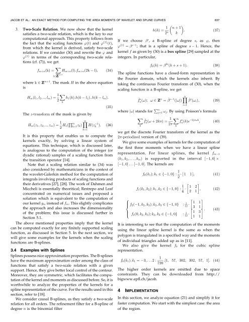
JACOB ET AL.: AN EXACT METHOD FOR COMPUTING THE AREA MOMENTS OF WAVELET AND SPLINE CURVES 6373. Two-Scale Relation. We now show that the kernelsatisfies a two-scale relation, which is the key to ourcomputational approach. This property follows fromthe fact that the scaling functions '…t† and ' f1g …t†,from which the kernel is derived, satisfy two-scalerelations. If we consider (30) and rewrite the ' and' f1gin terms of the corresponding two-scale relations(cf. (7)), we getf m‡n …k† ˆXl2 Z m‡1 H m‡n …l†:f m‡n …2k l†;…34†where k 2 Z m‡1 . The mask H in the above equationisXH m …l 1 ;l 2 ; ::; l m †ˆ1h 1 …k†:h…k l 1 †::h…k l m †:2k…35†The z-transform of the mask is given byH m …z 1 ;z 2 ; ::; z m †ˆ12 H 1… Q mkˆ1 z k† Ymkˆ1H…z 1k †: …36†It is this property that enables us to compute thekernels exactly, by solving a linear system ofequations. This technique, which is discussed later,is analogous to the computation of the integer (ordyadic rational) samples of a scaling function fromthe transition operator [14].Note that a scaling relation similar to (34) wasalso considered by mathematicians in the context ofthe wavelet-Galerkin method for the computation ofintegrals involving products of scaling functions andtheir derivatives [27], [28]. The work of Dahmen andMiccheli is essentially theoritical; Restrepo and Leafconcentrated on numerical issues and proposed asolution which is equivalent to the computation ofour kernel g m instead of f m . This slightly complicatesthe approach and also increases the dimensionalityof the problem; this issue is discussed further inSection 5.1.The above mentioned properties imply that the kernelcan be computed exactly for any finitely supported scalingfunction, as discussed in Section 5. In the next section, wewill give some examples for the kernels when the scalingfunctions are B-splines.3.4 Examples with SplinesSplines possess nice approximation properties. The B-splineshave the maximum approximation order among the class offunctions that satisfy a two-scale relation with a givensupport. Hence, they give better local control of the contour.Moreover, they are symmetric, which facilitates the computationof the kernel and moments as discussed before. So, it isworthwhile to analyze the properties of the kernels for aspline representation of the curve. For the results used in thissection, refer to [18].We consider causal B-splines, as they satisfy a two-scalerelation for all orders. The refinement filter for a B-spline ofdegree n is the binomial filterh…k† ˆ 1 n ‡ 12 n : …37†kIf we choose s , a B-spline of degree s, as ', then' f1g ˆ s1 ; that is a spline of degree s 1. Hence, thekernel f as given by (30) is a box spline [29] sampled at theintegers. In particular,f 0 …k† ˆ 2s …k ‡ s ‡ 1†:…38†The spline functions have a closed-form representation inthe Fourier domain, which the kernels also inherit. Bytaking the continuous Fourier transform of (30), when thescaling function is a B-spline, we get^f s n …!†; ! 2 Zn ˆ ^ s1 …j!j† Ynkiˆ1^ s …! i †;…39†where j!j stands for P njˆ1 ! j. By using Poisson's formulaX^f n s 1 X…! ‡ 2k† ˆ fn s 2…k†e2j!k ; …40†we get the discrete Fourier transform of the kernel as the2-periodized version of (39).We give some examples of kernels for the computation ofthe first three moments when we have a linear splinerepresentation. For linear splines, the kernel f m1…k 1 ;k 2 ; ...;k m † is supported in the interval ‰1; 0Š‰1; 0Š ...‰1; 0Š. The kernels arekf 0 …k 1 †; k 1 2f1; 0g : 1 ‰1 1Š; …41†2f 1 …k 1 ;k 2 †; k 1 ;k 2 2f1; 0g : 1 6 1 2; …42†2 18 f 2 …1;k 2 ;k 3 †; k 2 ;k 3 2f1; 0g : 1 12 1 1>:1 1…43†It is interesting to see that the computation of the momentsusing the linear spline kernel is the same as when thepolygon is triangulated in a specified way and the momentsof individual triangles added up as in [11].We also give the kernel f 0 for the cubic splinerepresentation.1f 0 …k 1 †; k 1 ˆ3; ...2: :‰1; 57; 302; 302; 57; 1Š: …44†720The higher order kernels are omitted due to spaceconstraints. They can be downloaded from http://bigwww.epfl.ch/jacob.4 IMPLEMENTATIONIn this section, we analyze equation (21) and simplify it forfaster computation. We start with the simplest case: the areaof the region.
Page 1 and 2: IEEE TRANSACTIONS ON PATTERN ANALYS
Page 3: JACOB ET AL.: AN EXACT METHOD FOR C
Page 7 and 8: JACOB ET AL.: AN EXACT METHOD FOR C
Page 9 and 10: JACOB ET AL.: AN EXACT METHOD FOR C

An exact method for computing the area moments of ... - IEEE Xplore

Create successful ePaper yourself

Delete template?

Save as template?