- Page 1 and 2: CEA DSM DAPNIA-02-395 (2002)ZGOUBI
- Page 3 and 4: Table of contentsPART A Description
- Page 5: PART ADescription of software conte
- Page 8 and 9: 8¤¥ PARTICUL Particle characteris
- Page 10 and 11: 10ELECTROMAGNETIC ELEMENTSDecapoleD
- Page 13 and 14: !!%" && 131 NUMERICAL CALCULATION
- Page 15 and 16: 1.2 Integration of the Lorentz Equa
- Page 17 and 18: 1.2 Integration of the Lorentz Equa
- Page 19: 4Ž ^ ˜ ¡§ ^"- ^ ˜ ¡ ^¡wTGT
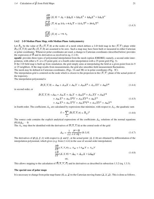
- Page 23 and 24: 4 ´ ´""4§> ´4 >4>1.4 Calculati
- Page 25 and 26: A cylindrically symmetric field can
- Page 27: Introducing also ¡The derivatives
- Page 30 and 31: 30 3 SYNCHROTRON RADIATION¾ÍôVT
- Page 32 and 33: 32 3 SYNCHROTRON RADIATIONÉ Éwher
- Page 35 and 36: 354 DESCRIPTION OF THE AVAILABLE PR
- Page 37 and 38: 4.2 Definition of an Object 37where
- Page 39 and 40: 4.2 Definition of an Object 39\Pqî
- Page 41 and 42: 4.2 Definition of an Object 41¹q
- Page 43 and 44: 4.3 Declaration of options 43\P4.3
- Page 45 and 46: 4.3 Declaration of options 45END or
- Page 47 and 48: 4.3 Declaration of options 47· £
- Page 49 and 50: 4.3 Declaration of options 49{ww{{q
- Page 51 and 52: 4.3 Declaration of options 51GASCAT
- Page 53 and 54: 4.3 Declaration of options 53·{N$
- Page 55 and 56: 4.3 Declaration of options 55PARTIC
- Page 57 and 58: 4.3 Declaration of options 57RESET:
- Page 59 and 60: 4.3 Declaration of options 59if qî
- Page 61 and 62: 4.3 Declaration of options 61P4©@4
- Page 63 and 64: 4.3 Declaration of options 63:£¨
- Page 65 and 66: u2 >04.4 Optical Elements and relat
- Page 67 and 68: 4.4 Optical Elements and related nu
- Page 69 and 70: 4.4 Optical Elements and related nu
- Page 71 and 72:
4.4 Optical Elements and related nu
- Page 73 and 74:
4.4 Optical Elements and related nu
- Page 75 and 76:
4.4 Optical Elements and related nu
- Page 77 and 78:
4.4 Optical Elements and related nu
- Page 79 and 80:
4.4 Optical Elements and related nu
- Page 81 and 82:
4.4 Optical Elements and related nu
- Page 83 and 84:
4.4 Optical Elements and related nu
- Page 85 and 86:
4.4 Optical Elements and related nu
- Page 87 and 88:
4.4 Optical Elements and related nu
- Page 89 and 90:
4.4 Optical Elements and related nu
- Page 91 and 92:
4.4 Optical Elements and related nu
- Page 93 and 94:
4.4 Optical Elements and related nu
- Page 95 and 96:
4.4 Optical Elements and related nu
- Page 97 and 98:
4.4 Optical Elements and related nu
- Page 99 and 100:
4.4 Optical Elements and related nu
- Page 101 and 102:
4.4 Optical Elements and related nu
- Page 103 and 104:
4.4 Optical Elements and related nu
- Page 105 and 106:
4.4 Optical Elements and related nu
- Page 107 and 108:
4.4 Optical Elements and related nu
- Page 109 and 110:
4.4 Optical Elements and related nu
- Page 111 and 112:
4.4 Optical Elements and related nu
- Page 113 and 114:
4.4 Optical Elements and related nu
- Page 115 and 116:
4.4 Optical Elements and related nu
- Page 117 and 118:
4.4 Optical Elements and related nu
- Page 119 and 120:
4.4 Optical Elements and related nu
- Page 121 and 122:
4.4 Optical Elements and related nu
- Page 123 and 124:
4.5 Output Procedures 123¨ ¢ < ¤
- Page 125 and 126:
4.5 Output Procedures 1254·444"4HI
- Page 127 and 128:
4.5 Output Procedures 127PICKUPS: B
- Page 129 and 130:
4.5 Output Procedures 129wSPNPRNL,
- Page 131 and 132:
4.5 Output Procedures 131TWISS: Cal
- Page 133 and 134:
4.6 Complementary Features 133U@©@
- Page 135:
4.6 Complementary Features 135¢ww@
- Page 139 and 140:
Keywords and input data formatting
- Page 141 and 142:
Keywords and input data formatting
- Page 143:
Keywords and input data formatting
- Page 146 and 147:
146 Keywords and input data formatt
- Page 148 and 149:
148 Keywords and input data formatt
- Page 150 and 151:
150 Keywords and input data formatt
- Page 152 and 153:
152 Keywords and input data formatt
- Page 154 and 155:
154 Keywords and input data formatt
- Page 156 and 157:
156 Keywords and input data formatt
- Page 158 and 159:
158 Keywords and input data formatt
- Page 160 and 161:
160 Keywords and input data formatt
- Page 162 and 163:
162 Keywords and input data formatt
- Page 164 and 165:
164 Keywords and input data formatt
- Page 166 and 167:
166 Keywords and input data formatt
- Page 168 and 169:
168 Keywords and input data formatt
- Page 170 and 171:
170 Keywords and input data formatt
- Page 172 and 173:
172 Keywords and input data formatt
- Page 174 and 175:
174 Keywords and input data formatt
- Page 176 and 177:
176 Keywords and input data formatt
- Page 178 and 179:
178 Keywords and input data formatt
- Page 180 and 181:
180 Keywords and input data formatt
- Page 182 and 183:
182 Keywords and input data formatt
- Page 184 and 185:
184 Keywords and input data formatt
- Page 186 and 187:
186 Keywords and input data formatt
- Page 188 and 189:
188 Keywords and input data formatt
- Page 190 and 191:
190 Keywords and input data formatt
- Page 192 and 193:
192 Keywords and input data formatt
- Page 194 and 195:
194 Keywords and input data formatt
- Page 196 and 197:
196 Keywords and input data formatt
- Page 198 and 199:
198 Keywords and input data formatt
- Page 200 and 201:
200 Keywords and input data formatt
- Page 202 and 203:
202 Keywords and input data formatt
- Page 204 and 205:
204 Keywords and input data formatt
- Page 206 and 207:
206 Keywords and input data formatt
- Page 208 and 209:
208 Keywords and input data formatt
- Page 210 and 211:
210 Keywords and input data formatt
- Page 212 and 213:
212 Keywords and input data formatt
- Page 214 and 215:
214 Keywords and input data formatt
- Page 216 and 217:
216 Keywords and input data formatt
- Page 218 and 219:
218 Keywords and input data formatt
- Page 220 and 221:
220 Keywords and input data formatt
- Page 222 and 223:
222 Keywords and input data formatt
- Page 224 and 225:
224 Keywords and input data formatt
- Page 226 and 227:
226 Keywords and input data formatt
- Page 228 and 229:
228 Keywords and input data formatt
- Page 231 and 232:
Examples 231oÑwü¦INTRODUCTIONSev
- Page 233 and 234:
2331 MONTE CARLO IMAGES IN SPES 2Fi
- Page 235 and 236:
235********************************
- Page 237 and 238:
237zgoubi data file.800 MeV/c KAON
- Page 239 and 240:
2393 IN-FLIGHT DECAY IN SPES 3Figur
- Page 241 and 242:
241Excerpt of zgoubi output : histo
- Page 243 and 244:
243Excerpt of zgoubi output : first
- Page 245 and 246:
245zgoubi data file (begining and e
- Page 247 and 248:
247zgoubi data file.MICROBEAM LINE,
- Page 249:
2499 HISTO HISTOGRAHISTOGRAMME DE L
- Page 253 and 254:
253INTRODUCTIONThe basic zgoubi FOR
- Page 255 and 256:
REFERENCES 255References[1] F. Méo
- Page 257 and 258:
Indexacceleration, 56, 58, 74, 155,