Lab 1: The metric system – measurement of length and weight

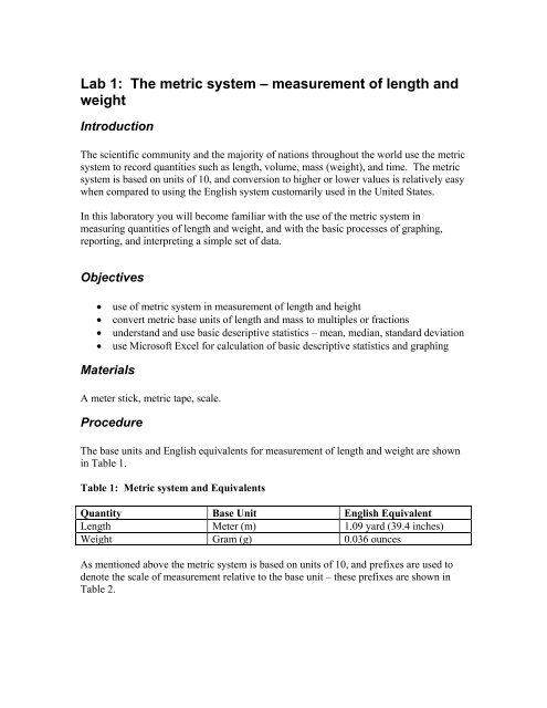
Table 2: Decimals of the metric systemPrefix Definition Multiple/fractionkilo- (k-) One thousand times greater 1000 fold of base unitdeci- (d-) One-tenth as much 0.1 of base unitcenti- (c-) One-hundredth as much 0.01 of base unitmilli- (m-) One-thousandth as much 0.001 of base unitmicro- (µ-) One-millionth as much 0.000001 of base unitFor example, the meter stick (1 m) you will be working with is composed of 100 cm or1000 mm. If you use the stick to measure your lab partner’s height and determine thatshe is 175 cm tall, you can equally report that her height is 1.75 m.Likewise if a student uses a metric scale to determine that he weighs 67.5 kilograms (kg),he can also report that his weigh is 67,500 grams, although the kg unit is moreappropriate to denote weights in this range. In another example a pill contains 250 mg ofibuprofen – this is equivalent to 0.25 g or 0.00025 kg – however reporting the weight inmilligrams (mg) is more appropriate for the quantity involved.1. Measurement of lower leg length and heightIn this part of the exercise you will measure lower leg length and body height of your labpartner.To measure lower leg length have your lab partner kneel on a chair with the thigh verticaland the back of the calf at a 90 degree angle to the thigh. Place a meter stick or tapealong the outside (lateral) edge of the back of his/her calf. You should feel the tendon ofthe biceps femoris muscle behind and on the lateral side of the knee. Make sure that themeter stick is just at the edge of the tendon, and record the distance in centimeters (cm)from this tendon to the bottom of his/her heel.To measure height have your partner take off his/her shoes and stand completely uprightagainst a wall. Place a hard cover book on top of his/her head and make a light mark onthe wall representing the top of the head – measure this distance in centimeters (cm) andconvert it to meters (m).Have your partner repeat the above procedures using you as a subject. When finishedenter the data for leg length (cm) and height (m) on the chalkboard or on a chart providedby your lab instructor.2. Descriptive statistics for class leg length and heightUsing Microsoft Excel you will determine the mean, median, and standard deviation forthe class leg length and height data collected above.

The mean is simply the mathematical average of the data. The mean provides you with aquick way of describing your data, and is probably the most used measure of centraltendency. However, the mean is greatly influenced by outliers. An outlier is anobservation in a data set which is far removed in value from the others in the data set. Itis an unusually large or an unusually small value compared to the others. For example,consider the following data set: 1, 1, 2, 4, 5, 5, 6, 6, 7, 150.While the mean for this data set is 18.7, it is obvious that nine out of ten of theobservation lie below the mean because of the large final observation. Consequently, themean is not always the best measure of central tendency.The median is the middle observation in a data set. That is, 50% of the observation areabove the median and 50% are below the median (for sets with an even number ofobservation, the median is the average of the middle two observation). The median isoften used when a data set includes outliers. In the example above the median is 5 – inthis example the median is a better measure of central tendency than the mean, due to thepresence of an outlier.Standard deviation is a measure of the spread or dispersion of a set of data. The morewidely the values are spread out, the larger the standard deviation. For example, say wehave two separate lists of exam results from a class of 30 students; one ranges from 31%to 98%, the other from 82% to 93%, then the standard deviation would be larger for theresults of the first exam.a. Open MS Excel by double clicking on the respective icon on the desktop of yourcomputer. The program will open and a window showing Workbook 1 will appear. Theworkbook is a spreadsheet with columns and rows that you will use to enter data. Eachindividual “rectangle” in the workbook is referred to as a “cell”.Columns are denoted alphabetically – A, B, C – and rows are identified numerically – 1,2, 3, etc. The location of a cell is indicated by its column and row coordinates – forexample, the cell located at the very top left of your screen is cell “A1”.b. Highlight cell B1 and type in “Height” – this is the title for the column where you willenter the data for class height you collected above. Highlight cell D1 and type in “Leglength” – this is the title for the column where you will enter the data for class leg lengthyou collected earlier.Get the data from the chalkboard and enter each individual data point in a cell – hit the“Enter” key or use the mouse to move the cursor to the next cell in the column.c. Descriptive statisticsGo to a cell below the last data point you entered in the column entitled “Height”.Highlight this cell and then click on the “=” sign on the upper left corner of the Exceltoolbar – a dialog box will appear.

Select the AVERAGE function from the scroll box on the left of this dialog box – asecond dialog box will open. In the text box following “Number 1” make sure that youlist the range of cells that you want to use to compute the average. For example, if“B2:B12” is listed in this text box, the function will compute an average using valuespresent in cells B2 – B12. Select OK. The function will now compute the average ormean for selected cells.Go to another cell below the “Height” column. Highlight this cell and then click on the“=” sign on the upper left corner of the Excel toolbar – a dialog box will appear.This time select the MEDIAN function from the scroll box on the left of this dialog box.Repeat the procedure outlined above to calculate the median for the height data.Go to another cell below the “Height” column. Highlight this cell and then click on the“=” sign on the upper left corner of the Excel toolbar – a dialog box will appear.This time select the STDEV function from the scroll box on the left of this dialog box.Repeat the procedure outlined above to calculate the standard deviation for the heightdata.Using the procedure outlined above determine the mean, median, and standard deviationfor the leg length data. Label cells so it is clear what the descriptive statistics refer to.Save the workbook to a folder indicated by your instructor.3. Relationship between leg length and heightUsing the class data collected above and Microsoft Excel, produce a graph that illustratesthe relationship between leg length and overall height of an individual. Plot the length ofthe leg (cm) on the x-axis and the overall height of the individual on the y-axis. Use thescatter plot feature of MS Excel and fit a line to the data. Print a copy of the graph andgive it to your instructor at the end of class (one copy per group). Save your work. Ageneral procedure for making scatter plots using MS Excel is outlined below.• Highlight all cells containing information. Then click Insert (in themain menu), then Chart.• Choose XY (Scatter) as a chart type. Then click Next.• On the next screen, click Next.• Fill in the Chart, X-axis, and Y-axis titles – include the units ofmeasurement in parentheses.• Click the tab labeled Legend. Uncheck the box labeled Show legend.• Click Next.• Click Finish

At this point you may note that the y-axis scale for your graph includes a range wherethere are no data points present. For example the shortest individual in the class was 1.58meters, yet the y-axis starts at zero. To correct this do the following:• Double-click on the y-axis.• On the dialog box that opens click the tab labeled Scale.• Change the minimum value to an appropriate number – in the aboveexample 1.50 meters would be appropriate.• Click OK• You may also have to adjust the scale of the x-axis in similar fashion.To add the line of best fit (trend line):• Choose Chart from the top menu bar. (Make sure that the graph ishighlighted/selected by box bullets on the perimeter. You can do thisby clicking anywhere on the graph.)• Click Add Trendline.• The Linear type of trend line should already be selected. This is whatyou need.• To get the R-Square value to print on your graph, click the tab labeledOptions. Then check the box titled Display R-Squared Value onChart.• Click OK.Note that R 2 indicates the strength of the relationship between the two variables. Valuesof R 2 ranges from 0 to 1.0. As the value of R 2 increases, the relationship is gettingstronger, with a value of 1.00 indicating a perfect correlation. Conversely, as R 2approaches 0, the correlation is weaker, with a score of 0 indicating the absence of anylinear relationship between the variables.4. Measurement of weightWeigh yourself either using a metric scale or a English scale. Enter your weight inkilograms (1 kg = 2.2 lb.) on the chalkboard or on a chart provided by your lab instructor.5. Descriptive statistics for class weightUsing the same MS Excel workbook you started earlier, create a new column for weightand enter the class values. Determine the mean, median, and standard deviation for thisvariable. Save your work. Print a copy of the Workbook and give it in to your instructorat the end of class (one copy per group).

6. Relationship between overall height and weightUsing the class data collected above and Microsoft Excel produce a graph that illustratesthe relationship between overall height and weight of an individual. Plot the overallheight (m) on the x-axis and the body weight (kg) of the individual on the y-axis. Use thescatter plot feature of MS Excel and fit a line to the data. Determine R 2 . Print a copy ofthe graph and give it to your instructor at the end of class (one copy per group). Saveyour work.

Assignment1. Conversions:1.76 m = _________ cm250 g = __________ kg375 mm = __________ m550 mg = _________ g2. Refer to the graph illustrating the relationship between leg length and height.a. Is there a correlation between leg length and height?b. For every 5 cm change in leg length what is the approximate change in height?c. According to your graph, predict how tall a person would be if his or her leg lengthwas 0.37 m. How tall do you predict they would be if the individual had a leg length of0.48 m?3. Refer to the graph illustrating a relationship between overall height and weight.a. Is there a correlation between height and weight?b. For every 2 cm change in height what is the approximate change in weight?c. According to your graph predict the weight of the individuals with the followingheights: (i) 185 cm; (ii) 140 cm

4. Which shows a higher degree of correlation, leg length and height or height and bodyweight? Explain your answer.5. If you were to do a new experiment examining the relationship between arm lengthand overall height, which of the two individuals below would you expect to be taller?Individual A: arm length = 65 cmIndividual B: arm length = 0.85 m