Tutorial for the WGCNA package for R - UCLA Human Genetics

More documents

Recommendations

Info

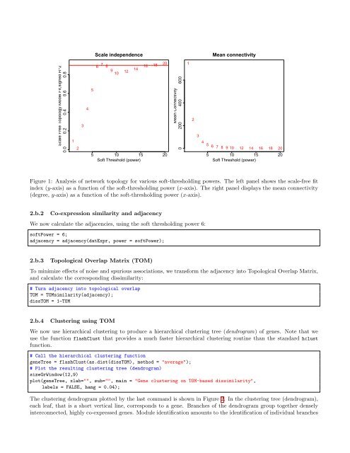
#The variable lnames contains the names of loaded variables.lnamesWe have loaded the variables datExpr and datTraits containing the expression and trait data, respectively.2 Step-by-step construction of the gene network and identification ofmodulesThis step is the bedrock of all network analyses using the WGCNA methodology. We present three different ways ofconstructing a network and identifying modules:a. Using a convenient 1-step network construction and module detection function, suitable for users wishing to arriveat the result with minimum effort;b. Step-by-step network construction and module detection for users who would like to experiment with customized/alternatemethods;c. An automatic block-wise network construction and module detection method for users who wish to analyze datasets too large to be analyzed all in one.In this tutorial section, we illustrate the step-by-step network construction and module detection.2.b Step-by-step network construction and module detection2.b.1Choosing the soft-thresholding power: analysis of network topologyConstructing a weighted gene network entails the choice of the soft thresholding power β to which co-expressionsimilarity is raised to calculate adjacency [1]. The authors of [1] have proposed to choose the soft thresholding powerbased on the criterion of approximate scale-free topology. We refer the reader to that work for more details; herewe illustrate the use of the function pickSoftThreshold that performs the analysis of network topology and aids theuser in choosing a proper soft-thresholding power. The user chooses a set of candidate powers (the function providessuitable default values), and the function returns a set of network indices that should be inspected, for example asfollows:# Choose a set of soft-thresholding powerspowers = c(c(1:10), seq(from = 12, to=20, by=2))# Call the network topology analysis functionsft = pickSoftThreshold(datExpr, powerVector = powers, verbose = 5)# Plot the results:sizeGrWindow(9, 5)par(mfrow = c(1,2));cex1 = 0.9;# Scale-free topology fit index as a function of the soft-thresholding powerplot(sft$fitIndices[,1], -sign(sft$fitIndices[,3])*sft$fitIndices[,2],xlab="Soft Threshold (power)",ylab="Scale Free Topology Model Fit,signed R^2",type="n",main = paste("Scale independence"));text(sft$fitIndices[,1], -sign(sft$fitIndices[,3])*sft$fitIndices[,2],labels=powers,cex=cex1,col="red");# this line corresponds to using an R^2 cut-off of habline(h=0.90,col="red")# Mean connectivity as a function of the soft-thresholding powerplot(sft$fitIndices[,1], sft$fitIndices[,5],xlab="Soft Threshold (power)",ylab="Mean Connectivity", type="n",main = paste("Mean connectivity"))text(sft$fitIndices[,1], sft$fitIndices[,5], labels=powers, cex=cex1,col="red")The result is shown in Fig. 1. We choose the power 6, which is the lowest power for which the scale-free topology fitindex reaches 0.90.
Scale independenceMean connectivityScale Free Topology Model Fit,signed R^20.0 0.2 0.4 0.6 0.81236 7 816 18209 141012545 10 15 20Soft Threshold (power)Mean Connectivity0 200 400 6001234 5 6 7 8 9 10 12 14 16 18 205 10 15 20Soft Threshold (power)Figure 1: Analysis of network topology for various soft-thresholding powers. The left panel shows the scale-free fitindex (y-axis) as a function of the soft-thresholding power (x-axis). The right panel displays the mean connectivity(degree, y-axis) as a function of the soft-thresholding power (x-axis).2.b.2Co-expression similarity and adjacencyWe now calculate the adjacencies, using the soft thresholding power 6:softPower = 6;adjacency = adjacency(datExpr, power = softPower);2.b.3Topological Overlap Matrix (TOM)To minimize effects of noise and spurious associations, we transform the adjacency into Topological Overlap Matrix,and calculate the corresponding dissimilarity:# Turn adjacency into topological overlapTOM = TOMsimilarity(adjacency);dissTOM = 1-TOM2.b.4Clustering using TOMWe now use hierarchical clustering to produce a hierarchical clustering tree (dendrogram) of genes. Note that weuse the function flashClust that provides a much faster hierarchical clustering routine than the standard hclustfunction.# Call the hierarchical clustering functiongeneTree = flashClust(as.dist(dissTOM), method = "average");# Plot the resulting clustering tree (dendrogram)sizeGrWindow(12,9)plot(geneTree, xlab="", sub="", main = "Gene clustering on TOM-based dissimilarity",labels = FALSE, hang = 0.04);The clustering dendrogram plotted by the last command is shown in Figure 2. In the clustering tree (dendrogram),each leaf, that is a short vertical line, corresponds to a gene. Branches of the dendrogram group together denselyinterconnected, highly co-expressed genes. Module identification amounts to the identification of individual branches
Page 1: Tutorial for the WGCNA package for
Page 5 and 6: The result is shown in Fig. 3.Gene
Page 7 and 8: Consensus clustering of consensus m

Tutorial for the WGCNA package for R - UCLA Human Genetics

You also want an ePaper? Increase the reach of your titles

Delete template?

Save as template?