Autonomous Mobile Robot Mechanical Design - the Dept. of ...

FACULTEIT Ingenieurswetenschappen
VAKGROEP Werktuigkunde
Autonomous Mobile Robot
Mechanical Design
Eindwerk ingediend tot het behalen van de academische graad
burgerlijk werktuigkundig-elektrotechnisch ingenieur
Kristof Goris
Academiejaar 2004-2005
Promotor: Prof. Dr. Ir. Dirk Lefeber
Co-Promotor: Prof. Dr. Ir. Hichem Sahli

Acknowledgements
Autonomous Mobile Robot: Mechanical Design
Many people have helped me along the way. Their guidance, good humour, advice
and inspiration sustained me trough the months of work. First of all, I’d like to thank
all of them.
Furthermore, I thank Mark and Guillermo for a nice cooperation during this project.
I wish to thank my promotors Prof. Dr. Ir. Dirk Lefeber and Prof. Dr. Ir. Hichem
Sahli for proposing this challenging project. And for their confidence in my abilities.
Many thanks go out to my supervisors, the support of Ir. Ronald Van Ham, Ir. Bram
Vanderborght, Ir. Thomas Geerinck, and Ir. Geert De Cubber kept me on the right
track during the year.
Many thanks go out to Jean-Paul Schepens, André Plasschaert, Gabriël Van den
Nest, Daniel Debondt, Eduard Schots and Thierry Lenoir for their technical support,
great work, and patience with me.
Furthermore, I wish to thank the WERK department for placing its infrastructure and
material at my disposal.
Finally I’d like to thank family and friends for being so supportive. I wouldn’t have
managed without them.
II

Executive Summaries
Autonomous Mobile Robot: Mechanical Design
Autonomous Mobile Robot: Mechanical Design
The design of autonomous mobile robots capable of intelligent motion and action
without requiring either a guide to follow or a teleoperator control involves the
integration of many different bodies of knowledge. This makes mobile robotics a
challenge worthwhile. To solve locomotion problems the mobile roboticist must
understand mechanisms and kinematics, dynamics and control theory. To create
robust perceptual systems, the mobile roboticist must leverage the fields of signal
analysis and specialized bodies of knowledge such as computer visions to properly
employ a multitude of sensor technologies. Localization and navigation demand
knowledge of computer algorithms, information theory, artificial intelligence, and
probability theory.
This thesis aims at building a locomotion mechanism that forms the base of a
complete mobile robot system capable of finding its way autonomously through a
path filled with obstacles. To accomplish this task, locomotion mechanisms and their
kinematics have to be studied, mechanisms have to be designed and developed. The
implementation of high and low level operating systems and electronics is required
as well to control the chassis’ motion.
III

Autonomous Mobile Robot: Mechanical Design
Autonome Mobiele Robot: Mechanisch Ontwerp
Het ontwerp van een autonome mobiele robot die in staat moet zijn intelligente
bewegingen en acties uit te voeren zonder hulp van een operator of gids, vereist de
integratie van verschillende technologieën. Dit maakt mobiele robotica
interdisciplinair en vervolgens een boeiende uitdaging. Om problemen op te lossen
omtrent beweging moet men kennis nemen van mechanica, kinematica, dynamica en
controle theorie. Robuuste gewaarwording systemen vereisen de kennis van signaal
analyse en computer beeldverwerking, evenals sensor technologieën. Plaatsbepaling
en navigatie vereisen computer algoritmes, informatie theorie, artificiële intelligentie
en waarschijnlijkheid theorie.
Het doel van deze thesis bestaat erin een bewegings mechanisme uit te werken dat de
basis vormt voor een complete mobiele robot die in staat is om zelfstandig zijn weg
te vinden doorheen een met obstakels gevulde ruimte. Hiertoe worden verscheidene
mogelijke bewegings mechanismen en hun kinematica bestudeerd, en mechanismen
worden ontworpen en ontwikkeld. Om de beweging van het chassis te controleren
worden bedieningssystemen en elektronica op verschillende niveaus
geïmplementeerd.
IV

Autonomous Mobile Robot: Mechanical Design
Le robot mobile autonome : le projet mécanique
L’ébauche d’un robot mobile autonome qui doit être capable de se mouvoir
intelligemment et d’exécuter des actions sans l’aide d’un opérateur ou d’un guide,
exige l’intégration de différentes technologies. Cela implique que la robotique
mobile devient interdisciplinaire et de ce fait un défi captivant. Pour résoudre des
problèmes de mouvement, la robotique mobile a besoin de la connaissance de la
mécanique, de la cinématique, de la dynamique et de la théorie de contrôle. Des
systèmes robustes de perception exigent la connaissance de l’analyse des signaux et
du traitement des images par ordinateur ainsi que des technologies de détection. La
localisation et la navigation exigent la connaissance des algorithmes informatiques,
la théorie d’information, l’intelligence artificielle et la théorie de probabilité.
Le but de cette thèse consiste à développer un mécanisme de mouvement qui est la
base d’un robot mobile complet capable de trouver son chemin d’une façon
autonome à travers un espace parsemé d’obstacles. Pour accomplir cette tâche, les
différents mécanismes de mouvements possibles et leur cinématique ont été étudiés
et des mécanismes ont été conçus et développés. Pour contrôler les mouvements du
châssis, des systèmes de commande et des systèmes électroniques sur différents
niveaux ont été mis en œuvre.
V

Contents
Autonomous Mobile Robot: Mechanical Design
Acknowledgements II
Executive Summaries III
1 Introduction 1
1.1 Objectives 1
1.2 Overview of the Thesis 2
2 Basic Concepts of Design 3
2.1 Introduction 3
2.2 Problem Statement 4
2.3 Definitions of Terms 5
2.3.1 Robot 5
2.3.2 Mobility 6
2.3.3 Autonomous 7
2.3.4 Holonomic and Non Holonomic 7
3 Wheeled Mobile Robots 9
3.1 Introduction 9
3.2 The Wheel and Rolling 11
3.2.1 Principle of Rolling 11
3.2.2 Wheel Classification 11
3.3 Wheel Configuration 14
3.3.1 Overview 14
3.3.2 Summary 27
4 Design and Development 28
4.1 Concept 28
4.1.1 General Dimensions and Robot Shape 29
4.1.2 Wheel Configuration and Wheels 30
4.1.3 Modularity 32
4.2 Energy Supply 34
4.2.1 Battery Pack 34
4.2.2 Case Study 36
4.2.3 Autonomy 37
4.2.4 Battery Charger 38
4.3 Mechanic design 39
4.3.1 Robot’s Leg 40
4.3.1.1 Driven Steered Standard Wheel 40
4.3.1.2 Bearings 45
4.3.2 Motors 46
4.3.2.1 Drive Motor 46
4.3.2.2 Steer Motor 49
4.3.3 Frame and Transmission 53
VI

Autonomous Mobile Robot: Mechanical Design
4.3.3.1 Frame 53
4.3.3.2 Transmission 55
4.4 Electronic design 58
4.4.1 Drive Motor Electronics 60
4.4.1.1 Inputs 61
4.4.1.2 Outputs 61
4.4.2 Steer Motor Electronics 62
4.4.2.1 Inputs 63
4.4.2.2 Outputs 63
4.4.3 Interface Electronics 64
4.4.3.1 Microcontroller 65
4.4.3.2 Voltage Regulation 65
4.4.3.3 Communication and Programming 66
4.4.3.4 Digital to Analogue Converter 66
4.4.3.5 Analogue to Digital Converter 66
4.5 Software design 67
5 Kinematics 72
5.1 Introduction 72
5.2 Kinematics 73
5.2.1 Representing Robot’s Position 73
5.2.2 Kinematic Wheel Model 75
5.2.3 Kinematic Robot Model 76
5.2.3.1 Degree of Mobility 78
5.2.3.2 Degree of Steerability 80
5.2.3.3 Degree of Manoeuvrability 81
5.2.4 Synchro Drive 81
6 Conclusions and Further Work 83
6.1 Conclusions 83
6.2 Further Work 84
Abbreviations 85
List of figures 86
References 88
Appendix A
Appendix B
VII

1 Introduction
1.1 Objectives
Introduction
The design of autonomous mobile robots capable of intelligent motion and action
involves the integration of many different bodies of knowledge. The aim of this
project is to idealise an existing autonomous mobile robot, on all levels. This
includes the mechanics, kinematics, dynamics, perception, sensor fusion,
localization, path planning and navigation. All these aspects have to be reviewed and
modified to a modular system, if necessary new modular modules have to be
designed and developed. This way a robust and modular autonomous mobile robot,
capable of intelligent motion and performing different tasks will arise. One of its
tasks could be winning the ‘Melexis Safety Throphy 2006’.
To obtain this aim, the workload is divided between three students. The thesis part of
Mark Nelissen is to write anew the software for the robot, making it also modular
and as independent of the hardware as possible. This consists of implementing last
year’s robot software, developed by Jan, Thomas and Bart [4], onto a new and
modular framework.
The thesis part of Guillermo Moreno is fully devoted to the development of a
modular sensor set up. This is designing the low level electronics and software in
charge of both controlling the different sensors hardware and saving the data
properly. Also a bus system, aimed at communicating with the on board PC,
supporting different sensor modules, is worked out.
This thesis will handle the problems concerning locomotion mechanisms, kinematics,
dynamics, and control and operating systems.
1

1.2 Overview of the Thesis
Introduction
In ‘chapter 2: Basic Design Concepts,’ some frequently used terms are explained and
the general approach to a mechanical design is given.
In order to take notice of the problems in the existing robot, and to be able to
idealise, or redesign a locomotion mechanism, a study is needed on the existing state-
of-the art locomotion mechanisms. This general study is presented in ‘Chapter 3:
Wheeled Mobile Robots.’ Different wheels and wheel configurations are discussed in
detail in this chapter.
The next chapter, ‘Chapter 4: Design and Development,’ is dedicated to the design
and development of a new locomotion mechanism, and the implementation of its
designed and developed electronics and operating software. This is the core chapter
of the thesis.
‘Chapter 5: Kinematics,’ deals with the in chapter 4 designed chassis’ kinematics.
Finally, conclusions are made and proposals for future work are enlightened in
‘Chapter 6: Conclusions and Further Work.’
2

2 Basic Design Concepts
2.1 Introduction
Basic Design Concepts
Mechanical engineering design is mainly a creative activity which involves a rational
decision making process. Generally speaking, it is directed at the satisfaction of a
particular need by means of a mechanical system, whose general configuration,
performance specifications and detailed definition conform the ultimate task of the
design activity.[7] There is no unified approach or methodology to actually design a
system, in so much as there does not exist a unified approach to creativity. Given a
particular need, each individual designer would probably design something different.
There are however, some common guidelines which can be useful in a very general
way. These guidelines are variations of the so called ‘design process’ (Fig.2.1),
which is a stepwise description of the main tasks typically developed in a
comprehensive design exercise. In any case, one of the main tasks in any design
situation is the so called ‘definition of the problem’ or ‘problem statement’.[7]
3

Basic Design Concepts
CONFONT NEED
REQUIREMENTS
PROPOSE CONCEPT
REDESIGN DESIGN SYSTEM
ANALYZE SYSTEM
REFINE DESIGN FABRICATE PROTOTYPE
2.2 Problem Statement
TEST PROTOTYPE
PRODUCTION PLANNING
PRODUCTION
END
Fig.2.1 A sequential Design Process [7]
What are the requirements? This is the main question to solve before designing a
mechanism. Wanted here is a robot platform modular in every way, and the
possibility to join the ‘Melexis Safety Trophy’ is desirable. To achieve this goal the
rules of the contest need to be known. These rules are a serious limitation of the
possibilities. A short overview is stated underneath. The challenge of the Melexis
Safety Trophy is to develop an autonomous robot that is able to drive safely from
point A to point B. The environment is similar to a real traffic situation with lanes,
road signs, traffic lights and other vehicles. More details about the concept and
4

Basic Design Concepts
specifications concerning the dimensions of tracks, lanes, road signs and obstacles
can be found in [5]. The robot’s most important specifications at this point are:
� Maximum and minimum dimensions; there is no maximal length, the width has
to be between 200mm and 450mm and the maximum height is 500mm.
� Drive; only electrical power is authorized, so no combustion engines may be
used.
� Locomotion; all robots need to use wheels. These wheels need to be big enough
to cope with small irregularities of the floor.
� Cost; the robot may not cost more than €2500. Borrowed or sponsored parts
count for their replacement value with exception of one personal computer or
laptop and one car battery, because these can be reused.
In order to construct a conform wheeled autonomous robot, some design decisions
have to be made. Before decisions can be made some terms have to be explained.
2.3 Definitions of Terms
2.3.1 Robot
A robot can be defined as ‘a mechanical device which performs automated tasks,
either according to direct human supervision, a pre-defined program or, a set of
general guidelines, using artificial intelligence techniques.’[1],[8] The first
commercial robot was developed in 1961 and used in the automotive industry by
Ford. The robots were principally intended to replace humans in monotonous, heavy
and hazardous processes. Nowadays, stimulated by economic reasons, industrial
robots are intensively used in a very wide variety of applications. Most of the
industrial robots are stationary. They operate from a fixed position and have limited
operating range. The surrounding area of the robot is usually designed in function of
5

Basic Design Concepts
the task of the robot and then secured from external influences. These robots
efficiently complete tasks such as welding, drilling, assembling, painting and
packaging.
However, in many applications it can be useful to build a robot which can operate
with larger mobility. In contrast to most stationary robots, where the surrounding
space is adapted to suit the robot tasks, mobile robots have to adapt their behaviour
to their surroundings. Instead of performing a fixed sequence of actions, mobile
robots need to develop some awareness of their environment through interaction with
all kind of sensors; they use on-board intelligence to determine the best action to
take. The development of intelligent navigation systems on mobile robots, which
ensures efficient and collision free movement, is still the centre of several research
projects. [1]
2.3.2 Mobility
Mobile robots are generally those robots which can move from place to place across
the ground. Mobility give a robot a much greater flexibility to perform new,
complex, exciting tasks. The world does not have to be modified to bring all needed
items within reach of the robot. The robots can move where needed. Fewer robots
can be used. Robots with mobility can perform more natural tasks in which the
environment is not designed specially for them. These robots can work in a human
centred space and cooperate with men by sharing a workspace together.[9]
A mobile robot needs locomotion mechanisms that enable it to move unbounded
throughout its environment. There is a large variety of possible ways to move which
makes the selection of a robot’s approach to locomotion an important aspect of
mobile robot design. Most of these locomotion mechanisms have been inspired by
their biological counterparts which are adapted to different environments and
purposes.[9],[10] Many biologically inspired robots walk, crawl, slither, and hop.
6

2.3.3 Autonomous
Basic Design Concepts
An autonomous robot is capable of detecting objects by means of sensors or cameras
and of processing this information into movement without a remote control.
2.3.4 Holonomic and Non Holonomic
In mobile robotics the terms omnidirectional, holonomic and non holonomic are
often used, a discussion of their use will be helpful.[9]
The terms holonomic and omnidirectional are sometimes used redundantly, often to
the confusion of both. Omnidirectional is a poorly defined term which simply means
the ability to move in any direction. Because of the planar nature of mobile robots,
the operational space they occupy contains only three dimensions which are most
commonly thought of as the x, y global position of a point on the robot and the
global orientation, θ, of the robot. Whether a robot is omnidirectional is not generally
agreed upon whether this is a two-dimensional direction, x, y or a three-dimensional
direction, x, y, θ.
In this context a non holonomic mobile robot has the following properties:
� The robot configuration is described by more than three coordinates. Three
values are needed to describe the location and orientation of the robot, while
others are needed to describe the internal geometry.
� The robot has two DOF, or three DOF with singularities. (One DOF is
kinematically possible but is it a robot then?)
In this context a holonomic mobile robot has the following properties:
� The robot configuration is described by three coordinates. The internal geometry
does not appear in the kinematic equations of the abstract mobile robot, so it can
be ignored.
7

Basic Design Concepts
� The robot has three DOF without singularities.
� The robot can instantly develop a wrench in an arbitrary combination of
directions x, y, θ.
� The robot can instantly accelerate in an arbitrary combination of directions x, y,
θ.
Non holonomic robots are most prevalent because of their simple design and ease of
control. By their nature, non holonomic mobile robots have fewer degrees of
freedom than holonomic mobile robots. These few actuated degrees of freedom in
non holonomic mobile robots are often either independently controllable or
mechanically decoupled, further simplifying the low-level control of the robot. Since
they have fewer degrees of freedom, there are certain motions they cannot perform.
This creates difficult problems for motion planning and implementation of reactive
behaviours.
Holonomic however, offer full mobility with the same number of degrees of freedom
as the environment. This makes path planning easier because there aren’t constraints
that need to be integrated. Implementing reactive behaviours is easy because there
are no constraints which limit the directions in which the robot can accelerate.
8

3 Wheeled Mobile Robots
3.1 Introduction
Wheeled Mobile Robots
Before we design and develop our own locomotion mechanism, we have to study the
existing mechanisms and compare their benefits an disadvantages.
Although a lot of locomotion mechanisms have been inspired by their biological
counterparts, nature did not develop a fully rotating, actively powered joint, which is
the technology necessary for wheeled locomotion. This mechanism is not completely
foreign to biological systems. Our bipedal walking system can be approximated by a
rolling polygon, with sides equal in length d to the span of the step, shown in
Fig.3.1.[10] As the step size decreases, the polygon approaches a circle or wheel. In
general, legged locomotion requires higher degrees of freedom and therefore greater
mechanical complexity than wheeled locomotion.[9]
Fig.3.1
A biped walking system can approximated by a
rolling polygon, with sides equal in length d to the
span of the step. As the step size decreases, the
polygon approaches a circle or wheel with radius l.
Fig.3.2
Specific power versus attainable speed of various
locomotion mechanisms
9

Wheeled Mobile Robots
The wheel has been by far the most popular locomotion mechanism in mobile
robotics and in man-made vehicles in general. It can achieve very good efficiencies,
as demonstrated in Fig.3.2 [10], and does so with a relatively simple mechanical
implementation. Wheels are extremely well suited for flat surfaces where this type of
locomotion is more efficient than a legged one. For example the railway is ideally
engineered for wheeled locomotion because rolling friction is minimized on a hard
and flat steel surface. When the surface becomes soft, wheeled locomotion
accumulates inefficiencies due to rolling friction whereas legged locomotion suffers
much less because it consists only of point contacts with the ground. This dramatic
loss of efficiency in the case of a tire on soft ground is also shown in Fig.3.2. [10]
Nature favours legged locomotion, because of its rough and unstructured terrain. In
contrast the human environment frequently consists of engineered, smooth surfaces,
both indoors and outdoors. Therefore virtually all industrial applications of mobile
robotics utilize some form of wheeled locomotion. In this thesis we shall not delve in
the theory concerning legged robots. We will however explain the wheel theory in
more detail since there is a very large space of possible kinds of wheels and their
configurations when one considers possible techniques for mobile robot locomotion.
10

3.2 The Wheel and Rolling
3.2.1 Principle of Rolling
Wheeled Mobile Robots
A wheel (as used here) is rotationally symmetric about its principal or roll axis and
rests on the ground on its contact patch. The contact patch is a small area which is in
frictional contact with the ground such that the forces required to cause relative
sliding between the wheel and ground are large for linear displacements and small
for rotational motions. Thus, we assume that a wheel undergoing pure rolling has a
contact point with no slip laterally or longitudinally, yet is free to twist about the
contact point. [9]
The kinematic constraint of rolling is called a higher-pair joint. The kinematic pair
has two constraints so that two degrees of freedom are lost by virtue of the rolling
constraint.
3.2.2 Wheel Classification
There are three major wheel classes. They differ widely in their kinematics, and
therefore the choice of wheel type has a large effect on the overall kinematics of the
mobile robot. The choice of wheel types for a mobile robot is strongly linked to the
choice of wheel arrangement, or wheel geometry. The mobile robot designer must
consider these two issues simultaneously when designing the locomotion mechanism
of a wheeled robot.
First of all there is the standard wheel as shown in Fig.3.3. This is what most people
think of when asked to picture a wheel. The standard wheel has a roll axis parallel to
the plane of the floor and can change orientation by rotating about an axis normal to
the ground through the contact point. The standard wheel has two DOF. A fixed
11

Wheeled Mobile Robots
Fig.3.3
Standard Wheels, from left to right: Fixed, Steered, Lateral Offset, Castor
standard wheel is mounted directly to the robot body. When the wheel is mounted on
a rotational link with the axis of rotation passing through the contact point, we speak
of a steered standard wheel. A variation which reduce rotational slip during steering
is called the lateral offset wheel. The wheel axis still intersects the roll axis but not at
the contact point. The caster offset standard wheel, also know as the castor wheel,
has a rotational link with a vertical steer axis skew to the roll axis. The key difference
between the fixed wheel and the castor wheel is that the fixed wheel can accomplish
a steering motion with no side effects, as the centre of rotation passes through the
contact patch with the ground, whereas the castor wheel rotates around an offset axis,
causing a force to be imparted to the robot chassis during steering.[9],[10]
The second type of wheel is the omnidirectional wheel. This is a disk with a
multitude of conventional standard wheels mounted on its periphery as shown in
Fig.3.4.[9] The omnidirectional wheel has tree DOF and functions as a normal
wheel, but provides low resistance in another direction as well. The angle of the
peripheral wheels may be changed to yield different properties. The small rollers
attached around the circumference of the wheel are passive and the wheel’s primary
axis serves as the only actively powered joint. The key advantage of this design is
that, although the wheel rotation is powered only along the one principal axis, the
12

Wheeled Mobile Robots
Fig.3.4
Omnidirectional Wheels, form left to right: Universal, Double Universal, Swedish 45°
wheel can kinematically move with very little friction along many possible
trajectories, not just forward and backward.[10]
The third type of wheel is the ball or spherical wheel. It has also three DOF. The
spherical wheel is a truly omnidirectional wheel, often designed so that it may be
actively powered to spin along any direction. There have not been many attempts to
build a mobile robot with ball wheels because of the difficulties in confining and
powering a sphere. One mechanism for implementing this spherical design imitates
the computer mouse, providing actively powered rollers that rest against the top
surface of the sphere and impart rotational force.[9][10]
13

3.3 Wheel Configuration
3.3.1 Overview
Wheeled Mobile Robots
The wheel type and wheel configuration are of tremendous importance, they form an
inseparable relation and they influence three fundamental characteristics of a:
manoeuvrability, controllability, and stability. In general there is an inverse
correlation between controllability and manoeuvrability.
The most popular wheel configurations are illustrated with an example below. The
used symbols are explained in Fig.3.5. The number of wheels rise from two to four
or more. A brief influence on stability, controllability and manoeuvrability is given
too.
Standard Fixed Wheel
Standard Driven Wheel
Standard Non Driven Steer Wheel
Standard Driven Steer Wheel
Omnidirectional Wheel
Castor Wheel
Linear Actuator
Fig.3.5
Legende
14

Wheeled Mobile Robots
Wheel configurations with two wheels are shown in Fig.3.6 and Fig.3.7 and in
Fig.3.8 and Fig.3.9. The first two-wheeled configuration is similar to the mechanism
of bikes, and motorcycles. At the front there is a steer wheel which enables the
change in orientation, and at the rear a powered drive wheel is mounted. This
configuration leads to a static instability when the mechanism is not driven.
Fig.3.6
Static unstable two-wheeled configuration
Fig.3.7
Bike
Surprisingly, the minimum number of wheels required for static stability is two. As
shown in Fig.3.8, a two-wheel differential drive robot can achieve static stability if
the centre of mass is below the wheel axle. However, under ordinary circumstances
such a solution requires wheel diameters that are impractically large. A commercial
mobile robot that uses this wheel configuration is shown in Fig.3.9.
15

Fig.3.8
Static stable two-wheeled configuration, if the centre
of mass is below the wheel axle
Wheeled Mobile Robots
Fig.3.9
Cye, a commercial two-wheel differential-drive robot
Conventionally, static stability requires a minimum of three wheels, with the
additional condition that the centre of gravity must be contained within the triangle
formed by the ground contact points of the wheels.
The differential drive is a two-wheeled drive system with independent actuators for
each wheel. The name refers to the fact that the motion vector of the robot is sum of
the independent wheel motions, something that is also true of the mechanical
differential. The drive wheels are usually placed on each side of the robot. A non
driven wheel, often a castor wheel, forms a tripod-like support structure for the body
of the robot. Unfortunately, castors can cause problems if the robot reverses its
direction. Then the castor wheel must turn half a circle and, in the process, the offset
swivel can impart an undesired motion vector to the robot. This may result in to a
translation heading error. Straight line motion is accomplished by turning the drive
wheels at the same rate in the same direction. That is not as easy as it sounds. In
16

Wheeled Mobile Robots
place rotation is done by turning the drive wheels at the same rate in the opposite
direction. Arbitrary motion paths can be implemented by dynamically modifying the
angular velocity and/or direction of the drive wheels. The benefits of this wheel
configuration is its simplicity. A differential drive system needs only two motors,
one for each drive wheel. Often the wheel is directly connected to the motor with
internal gear reduction. The robot described in [1],[2],[3] and [4] has this wheel
configuration. Despite is simplicity, the controllability is rather difficult. Especially
to make a differential drive robot move in a straight line. Since the drive wheels are
independent, if they are not turning at exactly the same rate the robot will veer to one
side. Making the drive motors turn at the same rate is a challenge due to slight
differences in the motors, friction differences in the drive trains, and friction
differences in the wheel-ground interface. To ensure that the robot is travelling in a
straight line, it may be necessary to adjust the motor speed very often. This may
require interrupt-based software and assembly language programming. It is also very
Fig.3.10
Differential drive configuration with two drive wheels and
a castor wheel
Fig.3.11
Khepera, a small differential drive robot
17

Wheeled Mobile Robots
important to have accurate information on wheel position. This usually comes from
the encoders. A round shape differential drive configuration is shown in Fig.3.10.
An other three-wheel configuration is the tri-cycle drive, shown in Fig.3.11 and
Fig.3.13. The difference between these two mechanisms are the way they steer and
drive. The first tri-cycle drive has a non driven steer wheel at the front/rear to change
orientation. The drive wheels are at the rear/front of the vehicle. A differential is
necessary when the wheels can not slip to avoid mechanical destruction. The second
tri-cycle drive has a combined steer and drive mechanism at the front/rear. Two free
wheels are mounted on the structure at the rear/front to maintain stability. It is up to
the robot designer to decide. Both possibilities have there benefits and disadvantages.
It is difficult to find a small differential, but it is also difficult to build a mechanism
that steers and drives at the same time. The tri-cycle drive has some serious
disadvantages common to the car drive configuration, those are explain later.
Fig.3.12
Tri-cycle drive, front/rear steering and rear/front driving
Fig.3.13
Piaggio mini truck
18

Fig.3.14
Tri-cycle drive, combined steering and driving.
Wheeled Mobile Robots
Fig.3.15
Neptune
Another three wheel configuration is the synchro drive. The synchro drive system is
a two motor drive configuration where one motor rotates all wheels together to
produce motion and the other motor turns all wheels to change direction. Using
separate motors for translation and wheel rotation guarantees straight line translation
when the rotation is not actuated. This mechanical guarantee of straight line motion
is a big advantage over the differential drive method where two motors must be
dynamically controlled to produce straight line motion. There is no need for interrupt
based control as in the case of differential drive method. Arbitrary motion paths can
be done by actuating both motors simultaneously. The mechanism which permits all
wheels to be driven by one motor and turned by another motor is fairly complex.
Wheel alignment is critical in this drive system, if the wheels are not parallel, the
robot will not translate in a straight line. In Fig.3.16 the synchro drive wheel
configuration is shown. Fig.3.17 shows MRV4 a robot with this drive mechanism.
19

Wheeled Mobile Robots
In order to improve stability the synchro drive system can be used with four wheels
as well.
Fig.3.16
Synchro drive wheel configuration.
Fig.3.17
MRV4 robot with synchro drive mechanism
Generally stability can be further improved by adding more wheels, although once
the number of contact points exceeds three, the hyper static nature of the geometry
will require some form of flexible suspension on uneven terrain to maintain wheel
contact with the ground. One of the simplest approaches to suspension is to design
flexibility into the wheel itself. For instance, in the case of some four wheeled indoor
robots that use castor wheels, manufacturers have applied a deformable tire of soft
rubber to the wheel to create a primitive suspension. Of course, this limited solution
cannot compete with a sophisticated suspension system in applications where the
robot needs a more dynamic suspension for significantly non flat terrain.
In addition, balance is not usually a research problem in wheeled robot designs,
because wheeled robots are almost always designed so that all wheels are in ground
contact at all times. Instead of worrying about balance, wheeled robot research tends
20

Wheeled Mobile Robots
to focus on the problems of traction and stability, manoeuvrability, and control. Can
the robot wheels provide sufficient traction and stability for the robot to cover all of
the desired terrain, and does the robot’s wheeled configuration enable sufficient
control over the velocity of the robot?
Consider the car type locomotion or Ackerman steering configuration used in
automobiles. It is very common in the ‘real world,’ but not as common in the ‘robot
world.’ The properties of the tri cycle drive are similar. Such a vehicle typically has a
turning diameter that is larger than the car. Furthermore, for such a vehicle to move
sideways requires a parking manoeuvre consisting of repeated changes in direction
forward and backward. The limited manoeuvrability of Ackerman steering has an
important advantage: its directionality and steering geometry provide it with very
good lateral stability in high-speed turns. The path planning is much more difficult.
Note that the difficulty of planning the system is relative to the environment. On a
highway, path planning is easy because the motion is mostly forward with no
absolute movement in the direction for which there is no direct actuation. However,
if the environment requires motion in the direction for which there is no direct
actuation, path planning is very hard. Ackerman steering and its cousin, tricycle
steering is characterized by a pair of driving wheels and a separate pair of steering
wheels (only a single steering wheel in tricycle locomotion as discussed above). In
Fig.3.18 a front wheel driven car drive is pictured. Its main concurrent is the rear
wheel driven car drive configuration and is shown in Fig.3.29. The differences
between these two kinds of Ackerman steering mechanisms are the same as the
differences between the two tri cycle drives explained a few paragraphs back in this
section. An advantage of front wheel drive is a smaller turning radius. However in
automobiles we see often the opposite. The construction of this combined drive and
steer train has great complexity.
21

Fig.3.18
Front driven/steered Ackerman steering
Wheeled Mobile Robots
Fig.3.19
Front steered/rear driven Ackerman steering
A car type drive is one of the simplest locomotion systems in which separate motors
control translation and turning this is a big advantage compared to the differential
drive system. There is one condition: the turning mechanism must be precisely
controlled. A small position error in the turning mechanism can cause large odometry
errors. This simplicity in in line motion is why this type of locomotion is popular for
human driven vehicles.
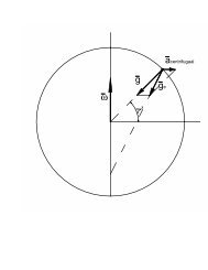
Articulated drive, as in Fig3.21, is similar to the car type drive except the turning
mechanism is a deformation in the chassis of the vehicle, not pivoting of wheels. By
deforming the chassis the forces act on the chassis, not on the steer train. This design
has the same disadvantages of the car-type drive. If multiple wheels are driven and a
differential is not used, wheel slippage will occur. This design is commonly used in
construction equipment (Fig3.22) where wheel slippage is not an issue because the
speeds are slow and the coefficient of friction with the ground is low. This type uses
22

Fig.3.21
Articulated drive configuration.
Wheeled Mobile Robots
Fig.3.22
Construction worker with articulated drive.
one motor to drive the wheels and one actuator to change the pivot angle of the
chassis.
23

Wheeled Mobile Robots
In the wheel configurations discussed above, we have made the assumption that
wheels are not allowed to skid against the surface. An alternative form of steering,
termed slip/skid, may he used to reorient the robot by spinning wheels that are facing
the same direction at different speeds or even opposite directions. There is no explicit
steering mechanism. Below in Fig.3.23 the mechanism is pictured. Skid-steer
locomotion is commonly used on tracked vehicles such as tanks and bulldozers, but
is also used on some four- and six-wheeled vehicles. The Nanokhod (Fig.3.24) is an
example of a mobile robot based on the same concept. Robots that make use of tread
have much larger ground contact patches, and this can significantly improve their
manoeuvrability in loose terrain compared to conventional wheeled designs.
However, due to this large ground contact patch, changing the orientation of the
robot usually requires a skidding turn, wherein a large portion of the track must slide
against the terrain. The disadvantage of such configurations is coupled to the
slip/skid steering. Because of the large amount of skidding during a turn, the exact
Fig.3.23
Slip/skid wheel configuration.
Fig.3.24
Nanokhod, an autonomous robot with tracks.
24

Wheeled Mobile Robots
centre of rotation of the robot is hard to predict and the exact change in position and
orientation is also subject to variations depending on the ground friction. Controlling
straight line travel can be difficult to achieve. Therefore, dead reckoning on such
robots is highly inaccurate. This is the trade off that is made in return for extremely
good manoeuvrability and traction over rough and loose terrain. Furthermore, a
slip/skid approach on a high-friction surface can quickly overcome the torque
capabilities of the motors being used. In terms of power efficiency, this approach is
reasonably efficient on loose terrain but extremely inefficient otherwise.
Some robots are omnidirectional, meaning that they can move at any time in any
direction along the ground plane (x, y) regardless of the orientation of the robot
around its vertical axis. This level of manoeuvrability requires omnidirectional
wheels which presents manufacturing challenges. Omnidirectional movement is of
great interest for complete manoeuvrability. Omnidirectional robots that are able to
move in any direction (x, y, θ) at any time are also holonomic as discussed in chapter
Fig.3.25
Omnidirectional configuration with three spherical
wheels
Fig.3.26
Robot with three omnidirectional wheels
25

Wheeled Mobile Robots
two. Two examples of such homonymic robots are presented below. The first
omnidirectional wheel configuration has three spherical wheels each actuated by one
motor, and there are placed in an equilateral triangle as depicted in Fig.3.26. This
concept provides excellent manoeuvrability and is simple in design however, it is
limited to flat surfaces and small loads, and it is quite difficult to find round wheels
with high friction coefficients. In general, the ground clearance of robots with
Swedish and spherical wheels is somewhat limited due to the mechanical constraints
of constructing omnidirectional wheels. The second omnidirectional wheel
configuration has four spherical wheels each driven by a separate motor. This
omnidirectional arrangement depicted in Fig.3.27 and Fig.3.28 has been used
successfully on several research robots. By varying the direction of rotation and
relative speeds of the four wheels, the robot can be moved along any trajectory in the
plane and, even more impressively, can simultaneously spin around its vertical axis.
For example, when all four wheels spin ‘forward’ or ‘backward’ the robot as a
Fig.3.27
Omnidirectional configuration with four spherical wheels
Fig.3.28
Uranus, a four omnidirectional wheeled robot
26

Wheeled Mobile Robots
whole moves in a straight line forward or backward, respectively. However, when
one diagonal pair of wheels is spun in the same direction and the other diagonal pair
is spun in the opposite direction, the robot moves laterally. This omnidirectional
wheel arrangement are not minimal in terms of control motors.
Even with all the benefits, few holonomic robots have been used by researchers
because of the problems introduced by the complexity of the mechanical design and
controllability.
3.3.2 Summary
En summary, there is no ‘ideal’ drive configuration that simultaneously maximizes
stability, manoeuvrability, and controllability. Each mobile robot application places
unique constraints on the robot design problem, and the designer’s task is to choose
the most appropriate drive configuration possible from among this space of
compromises. In the next chapter we will choose one wheel configuration and work
out a fully locomotion mechanism.
27

4 Design and Development
4.1 Concept
Design and Development
Before designing and developing a new robot platform, we will repeat our
requirements and our limitations. We want to build an autonomous mobile robot,
which will be used for different tasks in an indoor environment, and we must keep in
mind the possibility to join the ‘Melexis Safety Trophy.’ With the knowledge we
picked up in the previous chapters, we can design a new mechanical platform
conform our requirements that forms the base of the entire robot.
The robot is represented as a black box shown in Fig.4.1. In the first stage of the
design process the content of the black box is unknown. We just want the robot to
fulfil its tasks. Step by step we will refine the design and work out each different
module in the black box. The result, the final mechanical platform is also shown in
Fig.4.1.
Fig.4.1
Black box analogy and final mechanical platform
28

Design and Development
4.1.1 General Dimensions and Robot Shape
When the robot is desired to join the ‘Melexis Safety Trophy,’ the main limitations
are the dimensions and the cost of the robot. The maximum and minimum
dimensions are stated here:
� The maximum length Lmax is not determined.
� The maximum width Wmax is 450mm.
� The minimum width Wmin is 200mm.
� The maximum height Hmax is 500mm.
The shape of a mobile robot is of great importance and can have an impact on the
robots performance. For instance in Fig.4.2 a square and a cylindrical robot with
identical width are moving from left to right. The square robot has a greater risk of
being trapped by an obstacle or failing to finds its way through a narrow space. The
cylindrical robot can use a simple algorithm to find its way through the narrow
passage because it is able to rotate in front of the obstacle without getting trapped.
The square robot must back up first and rotate afterwards and even then it is
uncertain the robot is not getting trapped. Since we want to use the robot for different
tasks and the robot will run autonomously, a cylindrical shaped robot is the best
solution. The black box considering the general dimensions and the shape is shown
in Fig.4.3.
Fig.4.2
Cylindrical versus square robot shape
29

Design and Development
Fig.4.3
Black box analogy considering general dimensions and shape.
4.1.2 Wheel Configuration and Wheels
The next step in the design process is the choice of a wheel configuration and the
wheel types used in this wheel configuration. In chapter 3 an overview of possible
wheel configurations is given.
We decide to take a three wheeled synchro drive principle with standard steered
wheels. The standard wheels are chosen because of their simplicity and they
available in all sizes and shapes. In contrast omnidirectional wheels are complex and
hard to find.
The three wheeled synchro drive principle has some benefits with respect to other
wheel configurations, in this application. The main benefits:
30

Design and Development
� Only two motors are necessary; one motor rotates all wheels together to produce
motion, the other motor turns all wheels to change direction.
� No suspension needed; the three wheel configuration ensures the ground contact
of each wheel.
� The mechanical guarantee of straight line motion.
� The omnidirectional behaviour. The robot can move to a certain position, and
rotate in place to achieve a certain orientation.
� Possibility of symmetric design.
The main disadvantages:
� Complex mechanism which permits all wheels to be driven by one motor and
turned by another motor.
� Wheel alignment has to be precisely set to guarantee straight line motion.
There is however one problem with this configuration as we shall see in chapter 5. In
fact the robot chassis can only move from point to point and is not able to change its
orientation. If we want the robot to view the entire surrounded environment, we have
to equip the robot with a 360 degree sensor casing or hull.
31

4.1.3 Modularity
Design and Development
We decide to separate the robot into two parts as indicated in Fig.4.4. The inner
cylinder is the lower part of the robot which will become the mechanical platform
and is worked out further in this chapter. The bigger, surrounding cylinder will be
referred to as the upper part of the robot and will be the platform which can contain
the equipment needed to fulfil a desired robot task. In this way modularity is
introduced in the design phase. In our case the latter platform holds the computer,
camera, sensors and specific electronics and is mechanically coupled to the steering
motor. This means that when the steering motor is changing the orientation of the
wheels it changes the orientation of the upper platform identically.
Fig.4.4
Black box analogy, upper and lower platform
Now, to avoid a 360 degree sensor casing , we choose a simpler form, for example a
180 degree sensor casing, and attach it to the upper platform with an alignment in the
direction of motion, parallel with the wheels. This simplification avoids the more
expensive and more complicated 360 degree without losing too much of the robots
32

Design and Development
view. Although it might seem that the 360 degree sensor gives an overview of the
whole surrounding area, these images will still be fragmented and jump from one
sensor to the next which make image building quite a difficult task. By using the 180
degree sensor and aligning it with the wheels, a clear picture of the whole area is
yielded, just by rotating the robot around its axis. (Fig.4.5)
Sensor Casing
Fig.4.5
Synchro drive with attached sensor casing
In this application the upper platform contains a computer. A normal motherboard of
a PC with a PCI card on it is about 200mm high. This means that the upper platform
needs a height of 250mm to make sure the computer fits.
The sensors of the robot are sensors of the same type as used in previous work
[1],[2],[3] and [4]. These sensors and their specific wires and connections can be
placed in a 20mm deep housing. We decide to leave a 30mm wide shaft around the
mechanical platform to allow the sensor casing to move. The new dimensional
limitations are also shown in Fig.4.4.
33

4.2 Energy Supply
Design and Development
With this concept in mind, we can design the lower or mechanical platform. This
platform needs an energy supply to be able to perform tasks autonomously. Since
combustion engines are expelled of the ‘Melexis Safety Trophy’ we are forced to use
electrical energy. This energy is stored in accumulators or batteries. In fact there is a
difference between these terms, the first ones are rechargeable, the others are not. In
this thesis the terms are used redundantly, and we assume rechargeable batteries.
Choosing a battery configuration is a key feature in the design process. Actually this
is an iterative process. The dimensions, voltage, weight and recharge method of the
battery configuration form restrictions on the entire design process and determine
directly the autonomy of the robot.
4.2.1 Battery Pack
To achieve our requirements on energy supply we decide to make our own battery
pack. That way we can design a symmetric battery pack and increase the stability of
the robot. To increase the stability of the robot the centre of gravity should be located
as low as possible and on the normal axis through the centre of gravity of the triangle
formed by the three contact points of the wheels to the ground. The batteries make an
important contribution to the robots weight which we want to keep as low as
possible.
Nowadays a popular voltage seems to be 12V, used in automobiles and lots of other
applications. However, in the future the automobile industry intends to rise the
voltage from 12V to 24V or even to 36V because of the spectacular rise of electronics
in cars. We take 24V as an appeasement voltage.
34

Design and Development
A battery must meet certain performance goals. These goals include: quick discharge
and recharge capability, long cycle life (the number of discharges before becoming
unserviceable), low costs, recyclable, high specific energy (amount of usable energy,
measured in watt hours per kilogram), high energy density (amount of energy stored
per unit volume), specific power, and the ability to work in wide temperature range.
No battery currently available meets all these criteria.
However ‘Nickel Metal Hydride’ (NiMH) batteries fulfil this conditions quite well.
They have a high specific energy: around 90Wh/kg. Only ‘Lithium Ion’ batteries
score better with a specific energy around 150Wh/kg. But ‘Lithium Ion’ batteries are
very expensive, and hard to charge, a control unit is desirable. ‘Nickel Cadmium’
(NiCd) batteries are very similar to NiMH batteries. Both types of batteries have
higher specific energy and higher energy density than advanced ‘Lead Acid’
batteries. In Fig.4.6. a battery pack existing of twenty NiMH cells is shown.
a) b)
Fig.4.6
a) NIMH SPECIALE ACCU 13000F-1Z
b) Battery pack with twenty cells
35

The cell’s specifications are:
� Nickel Metal Hydride
� 1.2V
� 13000mAh
� 230g
� height 89mm, diameter 32.5mm
The entire battery pack’s specifications are:
Design and Development
� 20 × 1.
2V
= 24V
(4.1)
� 13000mAh
� 24 V × 13000mAh
= 312Wh
(4.2)
� 20 × 290g
= 5.
8kg
(4.3)
312
� specific energy; = 54kWh
/ kg
(4.4)
5.
8
� energy density;
20
312
2
× 0.
089×
0.
01625 × π
= 211kWh
/ m
3
(4.5)
� the specific arrangement of the cells will become clear in the rest of this chapter.
4.2.2 Case Study
Let us compare this battery pack with the one used in the mobile robot described in
previous work [1],[2],[3] and [4]. In the last application the robot had three 12V lead
acid batteries each with 6.5Ah. Two of those three batteries are connected serially.
The pack’s energy is:
24 × 6500 + 12 × 6500 = 234Wh
(4.6)
The new battery pack with his energy of 312 Wh gains 33% in energy.
36

Design and Development
The total weight of the three ‘Lead Acid’ batteries is almost 8kg. The specific energy
is around 30Wh/kg. The new battery pack gains almost 80%!
The energy density of the Lead batteries;
234
3
= 84kWh
/ m
3×
0.
15×
0.
065×
0.
095
(4.7)
When we compare (4.5) with (4.7) we see a factor 2.5 difference. This means two
and an halve time more energy in the same volume! Actually we loose some space
between the cells.
4.2.3 Autonomy
We can estimate the entire robot’s autonomy, when we estimate the power
consumption of each module. Assume the robot equipped with:
� PC, 100W
� 10 ultrasonic sensors (6500 Polaroid)[13], 10 × 5V
× 500mA
= 25W
The sensor has a peak current of 2000mA, the continuous current is 100mA, to
estimate the power consumption of the sensors we assume a mean current of
500mA.
� Electronic compass (Devantech)[14] 5 V × 15mA
= 75mW
� 10 infrared sensors (Sharp GP2D12)[15], 10 × 5V
× 50mA
= 2500mW
� Pan/Tilt camera (Sony EVI-D31)[16], 11W
� Motors, 100W
Hence in this chapter the two motors are discussed in more detail. In this
estimation we assume the power consumption of both motors 100W.
� Electronics, 15W
37

Design and Development
This estimation seems reasonable, it includes the loss in the motor amplifiers, and
interface electronics.
More details on the used sensors can be found in the specific datasheets.
When we add all estimated powers together we have a total power consumption of
254W. The autonomy of the robot equipped with the NiMH battery pack is then
312 Wh = 1.
2h
or 72min.
254W
4.2.4 Battery Charger
Charging self made battery packs is not obvious, especially not in this case. We need
a charge terminal that is able to charge twenty cells in one time. A charge terminal
with this capability is shown in Fig.4.7. This terminal is intended for charging NiCd
and NiMH storage battery packs consisting of 1 to 20 cells. The nominal capacity of
these storage battery types indicated in mAh is not important. This terminal can also
be used for charging standard Lead Acid storage batteries, Lead Fleece and Lead Gel
storage batteries if they consist of no more then 1 to 6 or 12 cells. The nominal
capacity of these storage battery types has to be within 500mAh to 100Ah. More
details on the charge terminal can be found in [17]. The charging time to charge the
NiMH battery pack is estimated between 6h-9h.
Fig.4.7
Charge Terminal 3000 [17]
38

4.3 Mechanic Design
Design and Development
Let us focus now on the mechanics in the lower platform and work out the proposed
concept. All parts of the lower platform are designed in ‘AutoDesk Inventor’ a
computer aided design (CAD) program. The technical drawings are appended in
appendix B. The designed parts are either developed by the VUB technicians, or they
are bought in specialised stores because of their complexity.
The proposed concept leads to a symmetric design (Fig.4.8) which will increase the
robot’s stability. We shall start with the steer and drive accommodation. In the
synchro drive configuration the mechanism to drive and to steer a single wheel is
repeated three times. Because these three mechanisms ensure the robot’s contact with
the ground, we will call the mechanisms the legs of the robot. Between the three legs,
there is some space to put the two motors necessary to drive the wheels and rotate all
legs and the upper platform. The specific motor electronics can also be placed
between the legs. The proposed battery pack has a symmetrical shape, and is fitted in
between the legs of the robot too. This explains the configuration of the battery pack.
Fig.4.8
Electronics
Black box analogy, symmetrical concept of the lower platform
Leg
Steer Motor
Drive Motor
39

4.3.1 Robot’s Leg
Design and Development
4.3.1.1 Driven Steered Standard Wheel
The robot’s legs are the most important assemblies of the mechanical platform and
they have three mayor functions. First of all the ground contact must be ensured. The
three legs together must be able to hold the entire weight of the robot. Secondly the
leg must act as a steered standard wheel. And finally the wheel has to be driven to
produce motion. Fig.4.9 shows the real leg, and a drawing of the leg made in
‘AutoDesk Inventor.’
Fig.4.9
Robot’s leg
40

Design and Development
The key part in the leg’s assembly is the right-angle driver as given in Fig.4.10. In
this device rotary power is transferred between two shafts at right-angles to each
other with transmission ratio 1:1. This part is bought because of its complexity.
Inside there are spiral bevel gears to reduce the backlash and to ensure a perfect gear
engagement and silent operation. The incoming and outgoing shaft both have large
bearings in deep races, and oil seal rings are fitted. The unit is filled with long-life
grease. The housing is a single-piece aluminium alloy casting with three flanges as
mounting points.
a) b)
Fig.4.10
a) Right-angle driver
b) Modified right-angle driver
This unit allows us to transfer the rotary power of the drive motor to the wheel in the
leg. The upper flange is removed for reasons that will be clear further in this section.
On the two parallel flanges a fork is mounted which contains the wheel spindle
(Fig4.11.a). Between the outgoing shaft (the lower one in Fig.4.10) and the wheel
spindle the transmission occurs with a small chain with a ratio 1:1. To reduce
inaccuracy and loss of exact wheel position a mechanism to tighten the chain is
necessary. Therefore the fork must be able to move up and down. The holes to mount
41

Design and Development
a) b) c)
Fig.4.11
a) Overview leg
b) Detail view of the fork with transmission and mechanism to tighten the small chain
c) Section view of the wheel spindle and detail view of the bearing housing
the fork to the right-angle driver are actually grooves to make this possible
(Fig.4.11.b). When the chain is tightened according specifications, the bolts and nuts
can screwed down to fix the fork.
In Fig.4.11.c the wheel spindle is shown. Inline skate wheels are used. These wheels
have always the same core, but can differ in size, shape, rebound, hardness and
moreover they are low cost. In the first design the possibility to change a wheel was
worked out. That way we were able to adapt the wheels on an easy way to the ground
the robot was riding on. To reduce the construction time the wheel is mounted fixed
on the spindle and preclude the possibility to change wheels easily. The figure
indicates also the ball bearing that supports the axle, and guarantees a smooth
rotation, and the way it is hold in its bearing housing with a locking washer. The
wheel spindle is also kept on its place by a smaller locking washer. That way the
wheel axle and bearings can not move axially anymore.
42

Design and Development
a) b)
Fig.4.12
a) Overview leg
b) Detail view of the assembly of the steer and drive mechanism
Let us focus now on how to make the leg a steered standard wheel. Fig.4.12.b shows
us the successive steps to achieve this. On the modified right-angle driver a part is
mounted, we will refer to this part as part X. In this part X the incoming shaft of the
driver is enlarged and enwrapped with a plain bearing to ensure smooth motion. Part
X has a lock bolt which is not visual on the figure. When this bolt is loose, we can
distort part X and the entire fork with the wheel in it. When we screw down the lock
bolt the two parts are fixed to each other. This distortion is needed to align the three
wheels as we shall see.
Over part X we place a rolling bearing. The top of part X is threaded. This way we
can screw down the bearing with a locking washer and a locking nut. On top of part
X we mount a chain wheel. Finally we mount a chain wheel with a hub on the
enlarged incoming shaft.
43

Design and Development
a) b) c)
Fig.4.13
a) Partial assembled leg
b) Bearing housing leg
c) Complete assembled leg
Now the partial assembly is placed in a bearing housing as in Fig.4.13.b. This
bearing housing exists of two parts screwed together with the rolling bearing
between them. The result is shown in Fig.4.13.c. This is a presentation of the entire
assembled leg which acts like a driven steered standard wheel. Assuming the bearing
house fixed; the wheel will rotate when we turn the upper chain wheel and the
orientation of the wheel will change when we turn the lower chain wheel.
44

4.3.1.2 Bearings
Design and Development
Before moving on to the motor choices we take a closer look at the used bearings in
the legs. The most important bearing in the leg is the bearing over part X. This
bearing is actually a double row angular contact ball bearing. In fact the bearing
corresponds in design to two single row angular contact ball bearings, but takes up
less axial space. Normally we need to place there two single row angular contact ball
bearings to support the axial forces due the weight of the robot. The axial force needs
to be absorbed in both directions because we do not want to lose the wheels when we
pick up the platform. This could happen when the leg weighs to heavy. When the
bearing can not hold the weight axially, then the bearing breaks and drops the wheel.
To solve this problem we have to use two similar bearings. When using two single
row angular contact bearings we have to place them back-to-back or face-to-face to
absorb the axial forces in both directions. We refer to [18] for more information. In
stead of these two bearings we us the double row angular contact ball bearing.
The bearing’s capabilities are actually exaggerated. But we were forced to take this
bearing because of the dimensions of the inner diameter. This bearing is equipped
with seals to keep the grease necessary for smooth rotary motion inside.
The bearing life is also exaggeratedly high, and can de calculated with the formulas
in [19]. We can assume the bearing working statically.
The smaller bearings used in the legs are just to support the wheel axle, and are
bearings similar to the bearings used in inline skate wheels. They need no further
comment.
All other bearings used in the whole mechanical platform are plain bearings. They
support or guide other parts and that way ensure smooth rotary motion.
45

4.3.2 Motors
4.3.2.1 Drive Motor
Design and Development
As we already know, there are two motors in the mechanical platform. First we
examine the drive motor. This motor must be able to drive the three wheels together
and produce motion in that way. To determine the needed power and torque of the
motor, we use a simple vehicle model as depicted in Fig.4.14.
FWeight
α Fg FN
Fig.4.14
Simple vehicle model
F = F + F
Pull
Weight
Friction
The vehicle with mass m is pulled onto a slope with an angle α with the horizontal.
The force needed to do this is called Fpull:
F = F + F
(4.8)
Pull
F Pull
Weight
Friction
= mg sinα + µ mg cosα
(4.9)
( sin α + µ cosα
)
FPull = mg
(4.10)
Appraisal rule of thumb values for motor selection are:
α = 15°
and µ = 0.
05
(4.11)
µ is an estimated friction coefficient of a rolling wheel.
46

Design and Development
The proposed mean speed in the ‘Melexis Safety Trophy’ is 2km/h or 0.56m/s. To be
sure the robot drives fast enough we assume a maximum speed of four times the
proposed mean speed:
v = 8km
/ h = 2.
2m
/ s
(4.12)
max
The power needed to drive the robot at a certain speed:
P pull ⋅
= F v
(4.13)
Pmax Fpull
⋅
= v
(4.14)
When we assume the robot’s mass 20kg we need a motor power of:
max
( + µ cos ) ⋅ v = W
P = mg α α 60
(4.15)
max
sin max
This value seems acceptable. Knowing that there are electrical steps with a motor of
100W, which are able to drive at a similar speed with an adult person on it. To be
sure about the calculated power an experiment was done to compare the
experimental motor power with the calculated motor power.
In this experiment a cart with a load of 20kg on similar wheels was pulled forward
with a drawing spring. The tractive pulling power to get motion was measured with
the spring. We noticed that the pulling force reduces once the cart is moving. We
took the highest measured value and we introduced a safety factor of four. The
experimental pulling force was then:
= C ⋅ F = 4 ⋅ 5N
= 20N
(4.16)
FPullExp Spring
When we put these value in (4.15) we get:
P = FPullExp
⋅v
= 20N
⋅ 2.
2m
/ s = 44W
(4.17)
max
The new estimated motor power seems also reasonable.
The motor torque is given by:
max
max
max
P = ω ⋅C
(4.18)
Pmax 2 N Motor Cmax
⋅
with NMotor the number of revolutions per second.
= π (4.19)
47

Design and Development
As we shall see the transmission ratio between the motor and the wheels is 1:1. We
can now calculate the NMotor as follows:
= 8km
/ h = 2.
2m
/ s = N 2 r
(4.21)
vmax Wheel π
v 2.
2
NWheel = N Motor = =
2πr
2π
0.
034
With (4.20) we can calculate the motor torque:
C
max
P
=
2πN
max
Motor
max ≈
44
= =
2π10
0.
7
Nm
10rps
(4.22)
(4.23)
The quest to a suitable motor can start now. We decide to try one of the motors used
in the robot described in [1],[2],[3],[4]. This motor fulfils the requirements.
Some motor specifications are:
� Assigned power rating, 70 W
� Nominal voltage, 18 V DC
� No load speed, 6610 rpm
To reduce the motor speed, and to increase the torque a gearbox is mounted on the
motor. The ratio of this planetary gearhead is 18:1. On the other side of the motor an
optical encoder is mounted. More details about the motor, gearhead and encoder can
be found in [20]. Fig.4.15 shows the used motor with gearhead and encoder.
Fig.4.15
Maxon motor (RE36) with gearhead GP32A(18:1) and encoder (HEDL5540)[20]
48

4.3.2.2 Steer Motor
Design and Development
The second, and last motor to choose is the steer motor. Two types of motors can be
considered for the steering task; stepper motors or servo motors. Let us compare
these two motor types.
Servo motors are standard DC or brushless motors with an encoder feedback loop.
As used in the drive application. The controller reads the position of the motor and
controls the power applied to the motor. Servo motors are faster moving point to
point and are better at accelerating very heavy loads than stepper motors. Servo
motors are more expensive than steppers, perhaps double the price, or more. They
are generally just as accurate, if maintained in a proper state of tune, however they
rely on encoders to provide positioning information back to the computer. Thus the
complexity of the system is at least doubled, with no accuracy advantage, greater
initial cost, and more maintenance issues.
Stepper motors are permanent magnetic motors that 'step' one increment each time
the controller gives its control electronics one pulse. This is done with the
assumption that the shaft rotates the specified number of steps. No realtime feedback
is provided to assure the motor maintains pace with the desired motion sequence.
Stepper motors are relatively inexpensive, and provide the same or greater accuracy
as servo motors. Sufficiently powerful stepper motors for a given application do not
lose steps. Stepper motors are no more likely to lose steps than a servo encoder is to
pass bad information back to the controller.
If for some reason a stepper motor does encounter an obstacle it can not overcome,
such as blocked wheels, it will simply skip steps, without harming anything. If a
servo motor encounters the same obstacle, it fight itself until it breaks a gear tooth or
burns up.
The ‘closed loop’ rhetoric sounds convincing to the uninitiated, but provides no
benefit over a simpler and cheaper reliable stepper system. That is why we decide to
49

Design and Development
take a stepper motor. In Fig.4.16 we see some specifications of the chosen stepper
motor. The stepper has a step angle of 0.9°.
Fig.4.16
Characteristics stepper motor [21]
It is not easy to calculate the requirements of a stepper motor, especially not when
the mechanism, in which the motor is used, is not determined yet. However these
formulas [21] can be used to compare the motor specifications with the requirements:
� Checking the running duty cycle;
A stepper motor is not intended to be run continuously with rated current. Lower
than 50% running duty cycle is recommended.
Running Time
Running Duty Cycle =
× 100
Running Time + Stopping Time
50

� Checking the Inertia Ratio;
Design and Development
Large inertia ratios cause large overshooting and overshooting during starting
and stopping, which can affect start-up times and settling times. Depending on
the on the conditions, operation may be impossible. With the following equation
we can check that the values found are below the reference inertia ratios given
by the constructor.
2
Total Inertia Of The Machine [ kgm ]
Inertia Ratio =
≤ 10
2
Rotor Inertia Of The Motor [ kgm ]
When this value is exceeded, we have to take a geared motor. Using a geared
motor can increase the drivable inertia load.
2
Total Inertia Of The Machine [ kgm ]
Inertia Ratio =
2
2
Rotor Inertia Of The Motor [ kgm ] × ( Gear Ratio)
� Checking the acceleration and deceleration rate;
≤ 10
Most controllers, when set for acceleration or deceleration, adjust the pulse
speed in steps. For that reason, operation may sometimes not be possible even
though it can be calculated. Calculate the acceleration/deceleration rate from the
following equation and check that the value is at or above the
acceleration/deceleration rate given by the constructor.
Accel / Decel Period [ ms]
Accel / Decel Rate =
Operating Pulse Speed [ Hz]
− Starting Pulse Speed [ Hz]
=
t
f − f
2
1 ≤
1
20
� Checking if the required torque falls within the pull-out torque of the speed-
torque characteristics. (Fig.4.16)
51

Design and Development
The first and the third condition present no problem in our application. The other two
conditions are hard to check. That is the reason why we opt for a stepper that is
probably too strong for this application. However this choice adds some modularity
in the whole concept because we are able to equip the upper platform with tools for
different tasks, and the stepper will probably still be able to turn the platform quite
fast. All this at a cost that is rather limited. Fig.4.17 shows the motor itself.
Fig.4.17
Vexta stepper motor (CSK268MBT)[21]
52

4.3.3 Frame and Transmission
4.3.3.1 Frame
Design and Development
In Fig.4.18 we see the blackbox analogy. The battery pack, the legs, and the motors
are already worked out. In this section we take a look at the frame of the mechanical
platform. This frame is the structure that holds all parts together.
Fig.4.18
Blackbox analogy
The main part in the frame is shown in Fig.4.19. Let us refer to this part as part Y
next in this section. Part Y is the biggest, and heaviest part but is quite easy to
construct. Most of the manufacture processes can be done with the lathe. Despite its
weight the stability stays assured, by placing this part in the centre of the mechanical
platform. This part is the base part of the mechanical platform and all other parts or
modules are attached on it. On the bottom of part Y a plate which hold the batteries
and electronics is screwed down and around part Y the three legs and two motors are
fixed.
53

Design and Development
Fig.4.19
Main socle and its inner parts
The wires specific to the motors and battery pack are lead away through the three
holes in the middle of the socle. In part Y we place first two plain bearings, one on
the bottom of the inner side, the other around the inner mantle (Fig.4.19). Next we
place a second part, part Z, inside the enveloped part Y. Finally we screw down a
plated chain wheel on top of part Z. Part Z can now freely rotate in part Y. It is on
part Z that the upper platform will be attached. We get (Fig.4.20):
Fig.4.20
Supporting frame
54

4.3.3.2 Transmission
Design and Development
There still rests us the transmission mechanism. We decide to transmit rotary motion
by chains. Other possibilities are belts or gears. Gears are heavy and take a lot of
space. The main disadvantage of belts is its slippage. It is very difficult to ensure the
parallel alignment, and to calculate the robot’s position when there is slippage. To
solve the problem of slippage we can opt for chains or teethed belts. Teethed Belts
and the specific pulleys are a good alternative way to transmit motion power. The
main disadvantage of a chain transmission is its backlash. This backlash is rather
limited by the small pitch (8mm) of the chains. Knowing that the chains backlash is
only two percent of the chain’s pitch, the backlash is acceptable in this application.
The chain transmission is also a bit smaller then a similar teethed belt transmission.
In an application where space is rather limited these facts can be convincing.
There are two large chains as shown in Fig.4.21. The first one, between the drive
motor and the three upper chain wheels of the legs, will be referred to as the upper
chain. The second one, between the steer motor and the lower chain wheels of the
legs, will be referred to as the lower chain. All transmission ratios are chosen 1:1.
a) b) c)
Fig.4.21
a) Transmission mechanism
b) Upper chain
c) Lower chain
55

Design and Development
The upper chain mechanism is quite easy. There is only one mechanism needed to
tighten the chain. The two small chain wheels shown in Fig.4.21 can slide to obtain
this. When the chain is tightened according specifications the small guiding chain
wheels are screwed down and loose their possibility to slide.
The lower chain needs such a slide system between every chain wheel of the leg, and
the chain wheel of the upper platform, to ensure the precise alignment. Remember all
wheels have to be aligned perfectly parallel to obtain straight line motion. This way
and the possibility to distort the wheel fork makes it able to align the wheels and the
upper platform. The second reason to add these slide mechanisms are to tighten the
chain.
When we put all parts so far together we have the finished mechanical platform
without electronics nor software (Fig.4.22). Notice, to limit the robot’s weight, all
parts are made of aluminium, except the connection parts to hold the legs motors and
chain assembly. These parts are in steel so they could be welded.
Fig.4.22
a) Mechanical platform and implementation transmission mechanism
56

Design and Development
b) Real mechanical platform
57

4.4 Electronic Design
Design and Development
Generally the control loop of the system is presented in Fig.4.23. We distinguish two
different loops. The left loop is closed by an operator. This means, it is the operator’s
task to react on the motion behaviour of the robot. When he/she decides to change
the motors’ set values the response will be visual in a different motion behaviour.
The right loop, is the loop of an autonomous system. There is no operator anymore to
decide the motors’ set values. In stead of the operators eyes, the robot itself must see
the motion behaviour and the possible consequences. This can be done by sensors.
Next it has to decide whether the motors’ set values need to be changed or not.
Notice the modules in the dotted square are the same in both control loops. When
these modules are worked out we can use the mechanical platform for different
applications.
The mechanisms in the mechanic module are already cleared out in the previous
section. There rests us to explain the steer and drive electronics and the software
modules. In this section we investigate the needed electronics, and the next section
will handle the software.
Operator
Computer (High Level Software)
Controller (Low Level Software)
Steer/Drive
Electronics
Mechanics
Motion Sensors
Fig.4.23
Control loops:
left loop with operator
right loop autonomous control with sensors
Sensor
Electronics
58

Design and Development
The mechanical platform contains only the electronics needed to drive and steer the
chassis. That way we limit also the wires and connectors through the socle, and we
limit the risks of twisted wires. The electronics needed to perform a well defined
task, such as sensors, the main computer and power supply distributing, are worked
out on the upper platform. We shall not discuss this modules in this thesis.
The mechanical platform contains three basic electronic modules as shown in
Fig.4.24. Let us take a closer look at each of these modules.
Fig.4.24
Three electronic modules used in the mechanical platform
59

4.4.1 Drive Motor Electronics
Design and Development
The first module we discuss is the drive motor amplifier. The ADS 50/5, shown in
Fig.4.25.a, is a servo amplifier for driving permanent magnet DC motors. Four
modes can be selected by DIP switches on the board:
� Speed control using tacho signals
� Speed control using encoder signals
� IxR compensated speed control
� Torque or current control
We decide to select the speed control using encoder signals, because the used motor
is equipped with an encoder. The amplifier has a wide input supply range. More
details on this device can be found in [22].
Of importance in this part of the design are the required inputs to drive the motor at a
certain speed, and the outputted information.
b) b)
Fig.4.25
a) Servo amplifier (ADS 50/5)[22]
b) Inputs and outputs
60

4.4.1.1 Inputs
Design and Development
Connectors one to five, shown in Fig.4.25.b at the left, are the power supply of the
motor, and the module itself.
The set value input (connectors one and two in Fig.4.25.b at the right) is wired as a
differential amplifier. The input voltage range is between –10V and +10V. There are
two possibilities[22]:
� Positive set value;
When the ‘+ Set Value’ > ‘- Set Value’ we apply negative motor voltage or
current and the motor shaft will turn counter clock wise (CCW).
� Negative set value;
When the ‘- Set Value’ > ‘+ Set Value’ we apply positive motor voltage or
current and the motor shaft will turn clock wise (CW).
When a voltage (between +4V and +50V) is given at ‘Enable’, connector three in the
figure, the servo amplifier will switch the motor voltage to the winding connections.
If the ‘Enable’ input is not switched on or is connected to the ‘Gnd’, the power stage
will be highly resistant and will be disabled.
4.4.1.2 Output
The speed monitor ‘Monitor n’, connector seven in the figure, is primarily intended
for the qualitative estimation of the dynamics. The absolute speed is determined by
the properties of the speed sensors and by the setting of the nmax potentiometer. The
output voltage of the speed monitor is proportional to the number of revolutions and
will be +10V or –10V, depending of the rotation direction, when the maximum
number of revolutions set by the nmax potentiometer has been reached.
61

4.4.2 Steer Motor Electronics
Design and Development
The second module is the steer motor amplifier. The CSK high-torque 2-phase
stepping motor unit (Fig.4.26.a) has two working modes[22]:
� One-pulse input mode;
When the ‘PULSE’ input is turned from ‘ON’ to ‘OFF’ while ‘DIR’ input is set
‘ON’, the motor will rotate one step CW. When the ‘PULSE’ input is turned
from ‘ON’ to ‘OFF’ while ‘DIR’ input is set ‘OFF’, the motor will rotate one
step CCW.
� Two-pulse input mode;
When the ‘CW’ input is turned from ‘ON’ to ‘OFF’ the motor will rotate one step
CW. When the ‘CCW’ input is turned from ‘ON’ to ‘OFF’ the motor will rotate
one step CCW.
We decide to take the one-pulse operating mode.
a) b)
Fig.4.26
a) Stepper amplifier (CSK 2-Phase)[22]
b) Inputs and outputs
62

4.4.2.1 Inputs
Design and Development
The six connectors on top of Fig.4.26.b are the stepper motor winding connectors.
Below them there are the power supply connectors. The supply is 24V or 36V with a
deviation of ten percent. We use 24V to supply the device.
The connectors ‘DIR./CCW’ are used in one-pulse mode to determine the motors
rotation sense. And finally the ‘PULSE/CW’ connector is used to determine the
steppers stepping frequency. An input is set ‘ON’ when there is applied a voltage of
5V. The motor behaviour is shown in Fig.4.27.
4.4.2.2 Outputs
Fig.4.27
One-pulse stepper motor operation[22]
The ‘TIMING’ signal indicates that the excitation of the motor is in the initial state.
The signal is outputted once each time the excitation sequence returns to the initial
state in synchronization with the input pulses. We do not use this output.
63

4.4.3 Interface Electronics
Design and Development
The third electronic module (Fig.4.28) is the interface between the computer and the
two motor amplifiers. In fact it has two very important task to fulfil. First of all it
communicates with the higher level systems, let us call this the computer. The
second task is to pass on the required amplifier input values. To obtain this
successfully, the PCB is equipped with a microcontroller. We shall refer to this
microcontroller as the low level control system. So when we speak of high level
control and high level software we mean everything that concerns the computer.
When we mention low level control and low level software, we deal with the
microcontroller. Let us take a closer look at the PCB.
8
3
9
1
Fig.4.28
7
3
Interface electronics
2
6 5
5
4
3
2
64

4.4.3.1 Microcontroller
Design and Development
The used microcontroller is a PIC16F877A. For all details about this PIC we refer to
the datasheets [23]. Our interests goes to the input and output possibilities, the clock
which is used , the memory, the possibility to save a program in its memory and the
instructions needed to program the controller. Some specifications of used PIC are:
� Operating Frequency: DC-20MHz
We use a crystal of 8MHz, this will be important in the software design.
� Flash Program Memory: 8K
� Data Memory (bytes): 368
� EEPROM Data Memory (bytes): 256
� Interrupts: 15
� Input/Output Ports: PortA, PortB, PortC, PortD, PortE
All these ports are used, however not entirely.
� Instruction Set: 35 instructions
This microcontroller is depicted in the dotted rectangle with number 1 in Fig.4.28.
4.4.3.2 Voltage Regulation
The incoming voltage of +24V is protected against inverse polarity, and is guide to
the DC-DC converter. A fuse must protect the entire board for short circuits. The
DC-DC converter converts the +24V into –12V and +12V.[24] These values are
needed for other components on the PCB. Further the +12V is converted to +5V and
a capacitor is used to removes the ripples. With the +5V we can supply the PIC and
some other components. All these voltage regulate and convert components are
shown in the dotted rectangles with number 2 in Fig.4.28.
65

Design and Development
4.4.3.3 Communication and Programming
In the dotted rectangles with number 3 in Fig.4.28, the communication components
are shown. The MAX232 chip [25] and PIC are used to communicate. There are
possibilities to communicate by serial connecter (Serial COM) and I 2 C bus. To load a
program we use the ‘In-Circuit Serial Programming pins’[23]. Switch ‘number 4’,
has to point away from the programming pins to be able to load the controller with a
program. After loading the switch has to be switched to put the PCB in operation
mode.
4.4.3.4 Digital to Analogue Converter
In order to get the desired ‘Set Value’ used in the servo amplifier, we use a DAC to
convert a byte into a voltage between –10V and +10V. The circuit is worked out in
the datasheets [24]. In Fig.4.28 number 5 corresponds with this circuit. The
potentiometers are used to tune the out coming voltage.
4.4.3.5 Analogue to Digital Converter
The same principle is used to read the speed of the drive motor. The in coming
voltage of ‘Monitor n’ is converted by a ADC to a byte. This circuit [25] is shown in
the figure by number 9.
The two bytes concerning the motor speed, and motor ‘set value’ are also made
visual by the LEDs (number 8).
The required data signals are available at connectors. Connector ‘number 6’ contains
the required servo amplifier signals, connector ‘number 7’ the stepper amplifier
signals.
66

4.5 Software Design
Design and Development
As mentioned in previous section we make a difference between the high level
software and the low level software. The low level software is more or less limited
by the limited instruction set to program the assembler code in the microcontroller.
Therefore we design a high level software module as well as a low level software
module. Fig.4.29 shows their relation.
PC-High Level Software (Driver.exe)
PIC-Low Level Software (Driver.asm)
Steer/Drive Electronics
Fig.4.29
Relationship high and low level software
Serial Communication
Integrated Circuit
Before we work out each software module, we explain what we require of the
software. We want to use the software as a interface between an operator and the
electronics. More specific we need a control panel, or an operating system which
make it possible to control the motion of the chassis. That is the high level software.
Next the computer needs to communicate with the PIC, and the PIC have to translate
it into usable bytes or signals and send it to the electronics. That is the low level
software.
The control panel made in ‘Visual Basic’ is shown in Fig.4.30. It contains two
sliders; the vertical slider determines a set value for the drive motor. When moving
the slider to the top, the chassis will drive faster and faster. When the slider is moved
to the bottom, the chassis will drive faster and faster in reverse direction. The second
67

Design and Development
slider determines a set value for the steer motor. When the slider is moved to the left,
the wheels’ orientation will change and the more the slider is moved to the left the
faster the wheels are turning. When we move the slider to the right the same will
happen but in opposite direction. The ‘Reset’ buttons will reset the specific slider and
the corresponding motion will disappear. When the ‘STOP’ button is pressed the
chassis will stop immediately. The ‘End’ button ends the application. The number
shown in the white boxes are the same numbers used in the high and low level
programs. The frequency of the stepper is visual even as the period to turn the wheels
a entire turn.
Fig.4.30
Control panel: Driver.exe
The program behind this control panel, just sends (by way of serial COM) four bytes
to the PIC microcontroller, and receives one byte which is send to the screen. Also
the bytes used in the assembler code are made visual. When the PIC receives
something the loop where it was working in becomes interrupted. In the interrupt the
received bytes are passed on and putted away in memory registers. The first and the
last bytes are respectively ‘11111111’ and ‘00000000’ and are used for
synchronisation. The two bytes between them are set values derived from the two
slider values. The value of the vertical slider (DriveIN1) is passed on without more
68

Design and Development
and goes from 1 to 255. The value of the horizontal slider is modified in the high
level program before it is sended to the PIC. The reason therefore, we want a
symmetric behaviour of the steer motor when we slide to the left or to the right. The
slider values are between ‘00000010’ and ‘11111110’. The corresponding decimal
numbers are respectively 2 and 254. The values after modification (StepIN1) are
shown in Fig.4.31.
Slider value (decimal): 2 - … - 127 – 128 – 129 - … - 254
Modified value (decimal): 2 - … - 127 – 1 – (127+128) - … - (2+128)
Fig.4.31
Values horizontal slider used in Driver.exe
For clearness’ sake following flow chart (Fig.4.32). The Dark grey box deals with
the high level program. The light grey boxes are at the low level, and the with boxes
are the out coming data signals. In the dotted rectangle the interrupt is shown. The
new values are copied and used when the loop in the main program (right side of the
figure) is reseted.
When the four bytes arrive in the PIC an interrupt will called on as mentioned. The
two data inputs of importance are copied in StepIN1 and DriveIN1. StepIN1 is
copied in StepIN2. Bit8 is checked and determines the rotating sense of the stepper.
Next the bits of DriveIN1 are switched, in other words bit1 becomes bit8, bit2
becomes bit7, and so on. The new byte is called DriveIN2, and is put on portB of the
PIC. This port is connected with the DAC. All these operations are done In the
interrupt. The DAC converts DriveIN2 into a voltage between –10V and +10V.
Let us take a look at the main program now.
69

DIR./CCW
‘ON’
4 bytes
(Driver.exe)
DataIN in
memory
StepIN?
DriveIN
Bit1-Bit8
DAC
DIR./CCW
‘OFF’
Design and Development
Fig.4.32
Flow chart
No
Yes
Set up
Reset Count
Block signal
Transmitter
?
Send DriveOut
Wait 5 ms
Increment
Count
Count =
StepIN?
Busy
PULSE
Wait 5 ms
70

Design and Development
First of all the PIC controller is initialised in the set up module. This means all input
and output directions are chosen, and the interrupt is initialised. After this we enter
the main loop of the program.
The main loop is a counter. Each count takes 2.5ms. The number we are counting to
is actually the value of StepIN2 without bit8, and is called StepIN3. When the
counter has reached this value, the counter resets, and a data signal is put on portA,
bit2. The signal (connected with PULSE) changes from ‘high’ to ‘low’ remains low
for 2.5ms and changes back from ‘low’ to ‘high’. This way we have made a block
signal with a variable frequency. The frequency is determined by the horizontal
slider on the control panel and lays between 3.125Hz and 133.3Hz. The frequency is
not linear but the period is! In the main loop we send also a byte back to the
computer, before doing this we check if the transmitter is busy or not. When it is
busy, we wait 5ms and try again to send the byte.
All different modules are now worked out, and can be implemented on the
mechanical platform. In the next chapter we take a closer look at the kinematics of
the developed mechanical platform.
71

5 Kinematics
5.1 Introduction
Kinematics
Kinematics is the study of the mathematics of motion without considering the forces
that affect the motion. Robot kinematics describes robot movements. We need to
understand the mechanical behaviour of the robot both in order to design the mobile
robot for desired tasks and to create control software for the mobile robot hardware.
The main question to be answered in this context is: ‘Given a certain steering angle
and a number of wheel turns, where will the robot end up and which way will it be
pointed?’ This problem is relatively simple. It deals with the geometric relationships
that influence the system, and with the relationship between control parameters and
the behaviour of a system in state space.
In robotics, the inverse problem is usually more interesting. Given that we want to
arrive to a certain position, oriented in a certain direction, the problem of inverse
kinematics is to compute the set of robot operations which will achieve the goal. The
solution to a inverse kinematic problem is almost always overdetermined.
Locomotion is the process of causing a mobile robot to move. In order to produce
motion, forces must be applied tot the vehicle. Dynamics is the study of motion in
which these forces are modelled. It deals with mass, force and speed associated with
these motions. The mobile robot is limited by dynamics. For instance, a high centre
of gravity limits the turning radius of a fast robot because of the danger of rolling.
72

5.2 Kinematics
Kinematics
Deriving a model [10] for the whole robot’s motion is a bottom-up process. Each
wheel imposes constraints on the robot’s motion. The kinematics of an individual
wheel an later the kinematics of the whole robot will be annotated but first a global
reference frame and the local reference frame is defined to represent the robot’s
position.
5.2.1 Representing Robot’s Position
In Fig.5.1 we model the robot as a rigid body on wheels, operating on a horizontal
YG YL
y P
θ
XL
x XG
Fig.5.1
Robot model as rigid body in global and local reference frame
73

Kinematics
plane. The global reference frame is given by the axes XG and YG an they define an
arbitrary inertial basis on the plane from some origin O. To specify the position of
the robot, we choose a point P on the robot chassis as its position reference point.
The basis defined by the axes XL and YL relative to P on the robot chassis is the
robot’s local reference frame. The position P in the global reference frame is given
by coordinates x and y. The angular difference between the two frames is given by θ.
We put these three elements in a vector ΦG :
⎡x
⎤
Φ
⎢ ⎥
G =
⎢
y
⎥
(5.1)
⎢⎣
θ ⎥⎦
This vector describes the robot’s posture in the global reference frame.
To describe the motion of the robot, it is necessary to map motion along the axes of
the global reference frame to motion along the axes of the robot’s local reference
frame. This mapping is function of the current pose of the robot, and is accomplished
using the orthogonal rotation matrix R:
⎡ cosθ
sinθ
0⎤
R =
⎢
⎥
⎢
− sinθ
cosθ
0
⎥
(5.2)
⎢⎣
0 0 1⎥⎦
The rotation matrix expresses the orientation of the base frame with respect to the
moving frame.
Given some velocity in the global reference frame {XG,YG} we can compute the
components of motion along the robot’s local axes XL and YL by:
Φ&
L = R(θ ) Φ&
G
(5.3)
A forward kinematic model would predict the robot’s overall speed in the global
reference frame. From equation (5.4) we can compute the global motion from the
local motion:
Φ&
−1 G = R(θ ) Φ&
L
(5.4)
74

5.2.2 Kinematic Wheel Model
Kinematics
The first step to a kinematic model is to express constraints on the motions of
individual wheels. Later these results are combined to compute the whole robot’s
motion. The synchro drive configuration has three steered standard wheels. Lets
focus on the kinematics of a steered standard wheel. A few assumptions are made to
simplify the equations. We assume:
� A movement on a horizontal plane.
� The steering axes orthogonal to the surface.
� The plane of the wheel remaining vertical.
� Point contact of the wheels.
� Pure rolling.
� No slippage.
� No friction for rotation around the contact point.
� That the wheels are not deformable.
� The wheels connected to the chassis.
Under these assumptions the wheel has two constraints. The first constraint enforces
the concept of rolling contact. This means that the wheel must roll when motion take
place in the appropriate direction. The second constraint enforces the concept of no
lateral slippage. This means that the wheel must not slide orthogonal to the wheel
plane.
A steered standard wheel connected to the chassis and its parameters is shown in
Fig.5.2. The position of the wheel in the local reference frame is given in polar
coordinates by the distance l and the angle α. The wheel can spin over time, and is
steerable, so β and φ are function of time t. Note that a fixed standard wheel has a
fixed steering angle β which is not function of time t.
75

YL
P α
l
Kinematics
v(t)
β(t)
The rolling constraint for the wheel is given by equation (5.5):
XL
r,ϕ(t)
Fig.5.2
Synchro drive with three steered standard wheels in local reference frame and its parameters
[ sin ( α + β ) − cos(
α + β ) − cos β ] R(
θ ) Φ&
− r & ϕ = 0
l G (5.5)
The first term denotes the total motion along the wheel plane, and must be equal to
the motion accomplished by the spinning wheel, ϕ&
r .
The sliding constraint for the wheel is given by equation (5.6):
[ cos ( β ) sin(
α + β ) l sin β ] R(
θ ) Φ&
= 0
α (5.6)
+ G
The component of the wheel’s motion orthogonal to the wheel plane must be zero.
5.2.3 Kinematic Robot Model
Now that we have a model for one steered standard wheel we can compute the
kinematic constraints of the whole robot chassis. Our chassis has three steered
standard wheels. However, the procedure to compute the kinematic robot model is
used for other wheel configurations as well. In general, given a robot with N standard
76

Kinematics
wheels, comprising Nf fixed and Ns steerable. Each standard wheel imposes
constraints on the robot motion. We can develop the equations for constraints in
matrix forms. The rolling constraints of all wheels can now be collected in a single
expression:
C R θ ) Φ& − C & ϕ = 0
(5.7)
R1
( G R2
⎡ CR1
f ⎤
with CR1 = ⎢
= CR1(
βs
( t))
(Nx3) (5.8)
CR1s
( βs
( t))
⎥
⎣ ⎦
⎡r1
f 0 ... ... ... 0 ⎤
⎢
⎥
⎢
0 ... 0 ... ... ...
⎥
⎢ ... 0 r
⎥
Nf 0 ... ...
CR
2 = ⎢
⎥ (NxN) (5.9)
⎢ ... ... 0 r1
s 0 ... ⎥
⎢ ... ... ... 0 ... 0 ⎥
⎢
⎥
⎢⎣
0 ... ... ... 0 rNs
⎥⎦
⎡ & ϕ f ( t)
⎤
& ϕ = ⎢ = & ϕ(
t)
& ϕs
( t)
⎥
(Nx1) (5.10)
⎣ ⎦
We use the same technique to collect the sliding constraints of all standard wheels
into a single expression with the same structure:
C
S R
( θ ) & = 0
(5.11)
Φ G
⎡ CSf
⎤
= ⎢ = C ( β ( t))
CSs
( β ( t))
⎥
(Nx3) (5.12)
⎣ ⎦
CS S
Next we can use the sliding constraints in conjunction with the rolling constraints to
generate analyses of the manoeuvrability of a robot chassis. The manoeuvrability is a
combination of the mobility available based on the sliding constraints plus additional
77

Kinematics
freedom contributed by the steering. First we define the degree of mobility, and the
degree of steerability, then the degree of manoeuvrability will follow.
5.2.3.1 Degree of Mobility
To satisfy equation (5.11), the motion vector R(θ ) Φ& must belong to the null space
of the projection matrix
equation (5.13) is true:
G
CS ( β ( t))
. This is the space N such that for any vector n in N
CS ( β ( t))
⋅ n = 0
(5.13)
If the kinematic constraints are to be honoured, then the motion of the robot must
always be within this space N. This can be demonstrated geometrically using the
concept of a robot’s ‘instantaneous centre of rotation.’
Consider a single standard wheel as in Fig.5.3.a. It is forced by equation (5.6) to
have zero lateral motion. We can show this geometrically by drawing a zero motion
line through its horizontal axis. At any given instant, wheel motion along the zero
motion line must be zero. More specific, the wheel must be moving instantaneously
along some circle of radius R such that the centre of that circle is located on the zero
motion line. This point is called the instantaneous centre of rotation, ICR. When R is
at infinity, the wheel moves in a straight line.
A vehicle can have several wheels, but it can have only one ICR. All of its zero
motion lines have to meet at a single point. Placing the ICR in this point gives the
single solution for robot motion. This is why the front wheels of a car have a
different steer angle as pictured in Fig.5.2.d. So with the geometric construction we
can see that the robot’s mobility is a function of the number of constraints of motion,
instead of the number of wheels.
For instance, in Fig.5.3.b and Fig.5.3.c two two-wheeled configurations are shown.
The first configuration, the bike type, has two lines of zero motion, because of each
wheel contributes a constraint. The two constraints are independent, and thus each
78

R
ICR
ICR
ICR
Kinematics
ICR
ICR
a) b) c) d)
Fig.5.3
Instantaneous Centre of Rotation for: a) Single standard wheel, b) Bike type, c) Differential drive, d) Car drive
further constraints overall robot motion. The second configuration is the differential
drive mechanism. The two wheels are aligned along the same horizontal axis. The
ICR lies along a line, not at a specific point. The second wheel imposes no additional
kinematic constraint on the robot motion since its zero motion line is identical to that
of the first wheel. Although both configurations have the same number of standard
wheels, the former has two independent kinematic constraints while the latter has
only one.
So, the robot chassis kinematics is therefore a function of the set of independent
constraints arising from all standard wheels. The mathematical interpretation of
independence is related to the rank of the matrix CS ( β ( t))
(5.12). The greater the
rank, the more constrained is the mobility. We can identify the possible range of rank
values for any robot. In general the robot has zero or more standard wheels, and zero
or more omnidirectional wheels. However, the omnidirectional wheels do not
contribute to the constraints of motion. A robot with only omnidirectional wheels has
rank zero. The maximum possible rank is three since the kinematic constraints are
specified along three degrees of freedom, or we can see that the constraint matrix has
three columns. So the possible rang of rank values is:
79

Kinematics
[ C ( ( )) ] 3
0 ≤ rank S β t ≤
(5.14)
Now we are ready to define a robot’s degree of mobility δm:
[ C ( β ( )) ]
δ = 3 − t
(5.15)
m
rank S
Consider a robot with only omnidirectional wheels. The rank is zero, and the degree
of mobility is three. In other words, there are no constraints on the chassis, such a
robot can directly manipulate all three degrees of freedom. The other extreme, a
robot with three independent constraints generated by three standard wheels, has
rank three, and its degree of mobility is zero. More specific, the robot is completely
constrained in all directions, and motion in the plane is totally impossible.
5.2.3.2 Degree of Steerability
The degree of mobility quantifies the degree of controllable freedom based on
changes to wheel velocity. Steering can also have an impact on a robot chassis. This
impact is indirect because after changing the angle of a steerable standard wheel, the
robot must move to have a impact on the robot’s pose. We can define the degree of
steerability δs as:
s
rank Ss
[ C ( β ( t))
]
δ = (5.16)
Note that we care about the number of independently controllable steering
parameters. In equation (5.12) we can see that CS ( β ( t))
includes CSs ( β ( t))
, this
means that a steered standards wheel can both decrease mobility and increase
steerability at once. The particular orientation of the steered standard wheel at any
instant imposes a kinematic constraint, but its ability to change that orientation can
lead to additional trajectories.
The range of the degree of steerability is:
0 ≤ δ s ≤ 2
(5.17)
80

Kinematics
When δ s is zero, the robot has no steerable standard wheels. When δ s is two, the
robot has no fixed standard wheels. For instance a pseudo bicycle in which both
wheels are steerable. It is possible to place the ICR anywhere on the ground plane
when δ s is two. Most robots have a single degree of steerability.
5.2.3.3 Degree of Manoeuvrability
With the degree if mobility δ m and the degree of steerability δ s we have all the tools
to compute the overall degree of freedom that a robot can manipulate. The degree of
manoeuvrability is defined as:
δ = δ + δ
(5.18)
M
m
s
The degree of manoeuvrability includes both the degree of freedom that the robot
manipulates directly through wheel velocity, and the degree of freedom that it
indirectly manipulates by changing the steering angle and moving.
5.2.4 Synchro Drive
Now we use the developed tools on our robot chassis. The robot has zero fixed
wheels, and three steered wheels. The three wheels do not share a common axle,
therefore two of the three contribute independent sliding constraints. The third must
be dependent on these two constraints for motion to be possible. The degree of
mobility is one. This is intuitively correct, the chassis with frozen steering angle of
the wheels can only move back and forth on a straight line. Based on equation (5.16)
the robot should have a degree of steerability of two. However in a synchro drive
principle a single motor steers all three wheels together. Therefore the system has an
extra constraint such that in reality the degree of steerability equals one. The
manoeuvrability based on these values equals two. This result implies that the
81

Kinematics
synchro drive can only manipulate two degrees of freedom. In fact there is no way to
change the chassis’ orientation, only the position on the plane can be manipulated.
In our case we add to possibility to change the orientation of the upper platform
when the robot is at rest because the upper platform is connected with the steering
motor. That way we have developed a non holonomic but omnidirectional robot
chassis.
82

Conclusions and Further Work
6 Conclusions and Further Work
6.1 Conclusions
In this thesis ‘Autonomous Mobile Robot: Mechanical Design’ a sub part of the
project ‘Autonomous Mobile Robot’, a locomotion mechanism is designed and
developed. This locomotion mechanism will form the chassis of an autonomous
mobile robot. The robot will be used in well structured engineered environments, on
flat surfaces, such as office buildings. In these circumstances a three wheeled,
cylindrical chassis will perform well. The three wheels ensure ground contact,
without the need of a complex suspension mechanisms. The shape, in combination
with omnidirectionality, avoids getting trapped easily. A symmetrical, cylindrical,
three wheeled configuration is worked out.
The designed chassis has a non holonomic behaviour. In fact the chassis’ orientation
can not be changed in direction. However, to create an omnidirectional system the
robot is divided into two parts. A mechanical, lower platform that is worked out in
this thesis, and an upper platform. The upper platform has to be mounted on a
specific part in the mechanical platform. This specific part is mechanically coupled
with the steer motor. That way we can orient the upper platform in any desired
direction when the robot is at rest, making the entire system omnidirectional.
Three driven steered standard wheels are used to produce motion. A chain
transmission is used to transmit the rotary power of the single drive motor to all three
the wheels. Another chain transmission transmits the rotary power of the single steer
motor to all three the wheels and the upper platform. That way the orientation of the
three wheels and the upper platform can be changed. Mechanisms to align easily the
three wheels and upper platform are implemented in the design.
The mechanical platform is also equipped with a microcontroller and specific motor
electronics. Interface electronics allows us to control the motors with the
83

Conclusions and Further Work
microcontroller. That way the mechanical platform, with its own energy supply,
more specific a battery pack, can be used individually for different applications.
To test the low level components, a high level operating and control system is
developed and can be used as a driver to control the motion of the mechanical
platform. After testing each module on its own, all modules were combined and the
motors were tested without load in a testing frame. These experiments were
successful.
Further Work
My fellow-students and I have worked out most of the major parts needed for the
desired autonomous mobile robot. However some more tests, the combining of the
different components and the last parts still have to be worked out before the robot
can actually be built to perform all its desired tasks.
Applied to the locomotion mechanism described in this work, some dynamic
experiments should be done to tune the mechanical platform even further and to
describe its dynamics. Unfortunately the time for this project was limited and these
data could not yet be obtained.
Also the upper platform still has to be worked out in more detail. As said before that
platform must contain the computer with the high level software and the sensor
casing needs to be fixed and aligned with the wheels to get a view of the
environment.
It is clear that there is still work to do and that all the efforts made in the different
fields will have to be combined to achieve the main aim: building an autonomous
mobile robot. Hence it becomes clear once again that robotics really is a challenging
and interdisciplinary field.
84

Abbreviations
Abbreviations
PC Personal Computer
CAD Computer Aided Design
DC Direct Current
CCW Counter Clock Wise
CW Clock Wise
PCB Printed Circuit Board
DAC Digital to Analogue Converter
ADC Analogue to Digital Converter
85

List of Figures
List of Figures
Fig.2.1 A sequential Design Process [7] 4
Fig.3.1 A biped walking system[10] 9
Fig.3.2 Specific power versus attainable speed of various 9
locomotion mechanisms[10]
Fig.3.3 Standard Wheels 12
Fig.3.4 Omnidirectional Wheels 13
Fig.3.5 Legend 14
Fig.3.6 Static unstable two-wheeled configuration 15
Fig.3.7 Bike 15
Fig.3.8 Static stable two-wheeled configuration, if the centre of mass 16
is below the wheel axle.
Fig.3.9 Cye, a commercial two-wheel differential-drive robot 16
Fig.3.10 Differential drive configuration with two drive wheels 17
and a castor wheel.
Fig.3.11 Khepera, a small differential drive robot. 17
Fig.3.12 Tri-cycle drive, front/rear steering and rear/front driving. 18
Fig.3.13 Piaggio mini truck 18
Fig.3.14 Tri-cycle drive, combined steering and driving 19
Fig.3.15 Neptune 19
Fig.3.16 Synchro drive wheel configuration 20
Fig.3.17 MRV4 robot with synchro drive mechanism 20
Fig.3.18 Front driven/steered Ackerman steering 22
Fig.3.19 Front steered/rear driven Ackerman steering 22
Fig.3.21 Articulated drive configuration 23
Fig.3.22 Construction worker with articulated drive 23
Fig.3.23 Slip/skid wheel configuration 24
Fig.3.24 Nanokhod, an autonomous robot with tracks 24
Fig.3.25 Omnidirectional configuration with three spherical wheels 25
Fig.3.26 Robot with three omnidirectional wheels 25
Fig.3.27 Omnidirectional configuration with four spherical wheels 26
Fig.3.28 Uranus, a four omnidirectional wheeled robot 26
Fig.4.1 Black box analogy and final mechanical platform 28
Fig.4.2 Cylindrical versus square robot shape 29
Fig.4.3 Black box analogy considering general dimensions and shape 30
Fig.4.4 Black box analogy, upper and lower platform 32
Fig.4.5 Synchro drive with attached sensor casing 33
Fig.4.6 a) NIMH SPECIALE ACCU 13000F-1Z 35
b) Battery pack with twenty cells
Fig.4.7 Charge Terminal 3000 [17] 38
Fig.4.8 Black box analogy, symmetrical concept of the lower platform 39
Fig.4.9 Robot’s leg 40
Fig.4.10 a) Right-angle driver 41
b) Modified right-angle driver
86

List of Figures
Fig.4.11 a) Overview leg 42
b) Detail view of the fork with transmission and mechanism
to tighten the small chain
c) Section view of the wheel spindle and detail view of the
bearing housing
Fig.4.12 a) Overview leg 43
b) Detail view of the assembly of the steer and drive mechanism
Fig.4.13 a) Partial assembled leg 44
b) Bearing housing leg
c) Complete assembled leg
Fig.4.14 Simple vehicle model 46
Fig.4.15 Maxon motor (RE36) with gearhead GP32A(18:1) 48
and encoder (HEDL5540)[20]
Fig.4.16 Characteristics stepper motor [21] 50
Fig.4.17 Vexta stepper motor (CSK268MBT)[21] 52
Fig.4.18 Blackbox analogy 53
Fig.4.19 Main socle and its inner parts 54
Fig.4.20 Supporting frame 54
Fig.4.21 a) Transmission mechanism 55
b) Upper chain
c) Lower chain
Fig.4.22 a) Mechanical platform and implementation transmission mechanism 56
b) Real mechanical platform
Fig.4.23 Control loops 58
Fig.4.24 Three electronic modules used in the mechanical platform 59
Fig.4.25 a) Servo amplifier (ADS 50/5) 60
b) Inputs and outputs
Fig.4.26 a) Stepper amplifier (CSK 2-Phase)[22] 62
b) Inputs and outputs
Fig.4.27 One-pulse stepper motor operation[22] 63
Fig.4.28 Interface electronics 64
Fig.4.29 Relationship high and low level software 67
Fig.4.30 Control panel: Driver.exe 68
Fig.4.31 Values horizontal slider used in Driver.exe 69
Fig.4.32 Flow chart 70
Fig.5.1 Robot model as rigid body in global and local reference frame 73
Fig.5.2 Synchro drive with three steered standard wheels in local 76
reference frame and its parameters
Fig.5.3 Instantaneous Centre of Rotation for: a) Single standard wheel, 79
b) Bike type, c) Differential drive, d) Car drive
87

References
References
[1] J. Defever B. Francis and T. Geerinck, “Mobile Robots with Shared Autonomy”,
Vrije Universiteit Brussel, Brussels, Belgium, 2004
[2] J.Defever “Mobile Robots with Shared Autonomy: Navigation Control”,
Vrije Universiteit Brussel, Brussels, Belgium, 2004
[3] B.Francis, “Mobile Robots with Shared Autonomy: Visual Sevoing”,
Vrije Universiteit Brussel, Brussels, Belgium, 2004
[4] T. Geerinck, “Mobile Robots with Shared Autonomy: Tele-Robotics”,
Vrije Universiteit Brussel, Brussels, Belgium, 2004
[5] NN, “Competition rules Melexis Safety Trophy”,
http://www.trophy.melexis.com/, Belgium, 2005
[6] I.J. Cox G.T. Wilfong, “Autonomous Mobile Vehicles”, NEC Research Institute
QT&T Bell Laboratories, Princeton, Murray Hill, USA, 1990
[7] Victor H. Mucino, “Computer Aided Design Through Engineering Case Studies”,
College of Engineering and Mineral Resources, West Virginia University,
West Virginia, 1997
[8] P. Kool, “Robotica”, Vrije Universiteit Brussel, Brussels, Belgium, 2000
[9] Robert Holmberg, “Design and Development of Powered-Castor Holonomic
Mobile Robots”, Stanford University, 2000
[10] Roland Siegwart, Illah R. Nourbakhsh “Introduction to Autonomous Mobile
Robots”, The MIT Press, Massachusetts Institute of Technology, Cambridge,
Massachusetts, 2004
[11] Mike Ashby, Kara Johnson “Materials and Design”, Butterworth-Heinemann, Oxford,
2002
[12] Mike Ashby, “Materials Selection in Design”, Butterworth-Heinemann, Oxford, 1999
[13] Datasheet, “ultra sonic sensor 6500 Polaroid”, www.robotstorehk.com/6500.pfd
[14] Datasheet, “digital compass Devantech”, www.robot-electronics.co.uk/
[15] Datasheet, “Infrared sensor Sharp GP2D12”,
www.zuff.info/SharpGP2D12_E.html
[16] Datasheet, “pan/tilt camera Sony EVI-D31”,
www.picturephone.com/pdf/sony_evid30.pdf
[17] Datasheet, “Charge Terminal 3000”, www.conrad.com
[18] NN, “SKF angular contact ball bearings-your key to longer service life”, SKF,
www.skf.com, 2002
[19] NN, “SKF General Catalogue”, SKF, Germany, 2005
[20] Datasheet, “Maxon motor RE36”, www.maxonmotor.com
[21] Datasheet, “Vexta Stepper CSK 2-phase”, www.orientalmotors.com
[22] Datasheet, “Maxon servo amplifier ADS 50/5”, www.maxonmotor.com
[23] Datasheet, “PIC16F87XA Data Sheet”, www.microchip.com
[24] Datasheet, “Traco Power DC/DC-Konverter TEN4Serie”, www.tracopower.com
[25] Datasheet, “MAX232”, www.maxim-ic.com
[26] Datasheet, “8-bit high-speed multiplying D/A Converter”,
www.philipssemiconductors.com
[27] Datasheet, “Microcontroller Compatible 8-bit A/D Convertor”, www.maxim-ic.com
88