Optimization of a Microstrip Matching Circuit at ... - Sonnet Software

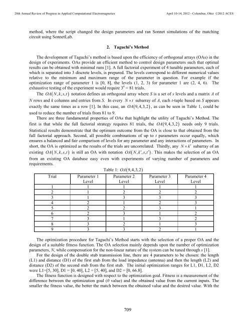
28th Annual Review of Progress in Applied Computational ElectromagneticsApril 10-14, 2012 - Columbus, Ohio ©2012 ACESmethod, where the script changed the design parameters and ran Sonnet simulations of the matchingcircuit using SonnetLab.2. Taguchi’s MethodThe development of Taguchi’s method is based upon the efficiency of orthogonal arrays (OAs) in thedesign of experiments. OAs provide an efficient method to control design parameters such that optimalresults can be obtained with minimal runs [1]. A full factorial experiment of 4 tunable parameters, each ofwhich is separated into 3 discrete levels, is prepared. The levels correspond to different numerical valuesrelative to the minimum and maximum range of the parameter in question. For example if theoptimization range of parameter 1 is [0, 8], the levels (1, 2, 3) for parameter 1 are (2, 4, 6). Theexhaustive testing of the experiment would require 3 4 = 81 trials.The OA( N, k, s,t ) notation defines an orthogonal array where S is a set of s levels and a matrix A ofN rows and k columns and entries from S. In every N× t subarray of A, each t-tuple based on S appearsexactly the same times as a row [1]. In this case, an OA ( 9,4,3,2), as can be seen in Table 1, could beused to reduce the number of trials from 81 to 9.There are three fundamental properties of OAs that highlight the utility of Taguchi’s Method. Thefirst is that while the full factorial strategy requires 81 trials, the OA ( 9,4,3,2)needs only 9 trials.Statistical results demonstrate that the optimum outcome from the OA is close to that obtained from thefull factorial approach. Second, all possible combinations of up to t parameters occur equally, whichensures a balanced and fair comparison of levels for any parameter and any interactions of parameters. Inshort, the OA is optimized as the results of the trials are uncorrelated. Thirdly, any N× k′ subarray of anexisting OA( N, k, s,t ) is still an OA with notation OA( N, k′ , s,t′ ) . This makes the selection of an OAfrom an existing OA database easy even with experiments of varying number of parameters andrequirements.Table 1: OA ( 9,4,3,2)Trial Parameter 1LevelParameter 2LevelParameter 3LevelParameter 4Level1 1 1 1 12 1 2 2 23 1 3 3 34 2 1 2 35 2 2 3 16 2 3 1 27 3 1 3 28 3 2 1 39 3 3 2 1The optimization procedure for Taguchi’s Method starts with the selection of a proper OA and thedesign of a suitable fitness function. The OA selection mainly depends upon the number of optimizationparameters, N, while compensation for the non-linear nature of the system can be tuned through s [1].For the design of the double stub transmission line, there are 4 parameters to be chosen: the length(L1) and distance (D1) of the first stub from the load impedance (antenna) and then the length (L2) anddistance (D2) of the second stub from the first stub. The initial optimization ranges for L1, D1, L2, D2were L1=[5, 30], D1 = [0, 40], L2 = [5, 40], and D2 = [0, 66.8].The fitness function is designed with respect to the optimization goal. Fitness is a measurement of thedifference between the optimization goal (0 value) and the obtained value from the current inputs. Thesmaller the fitness value, the better the match between the obtained value and the desired value. With the709