Optimization of a Microstrip Matching Circuit at ... - Sonnet Software

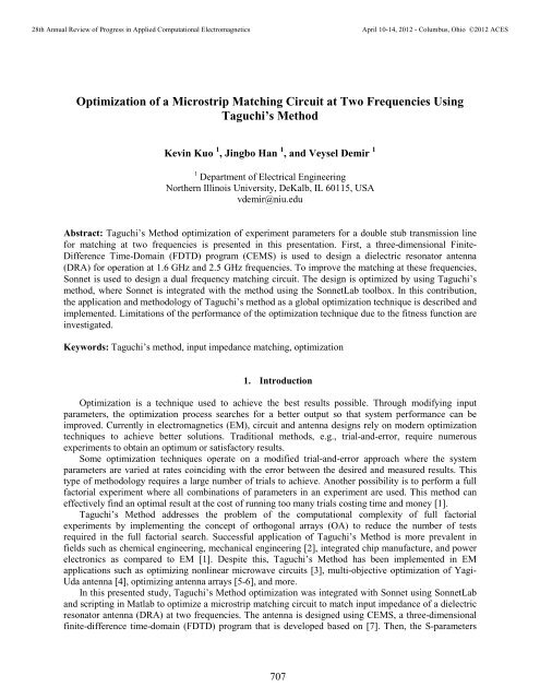
28th Annual Review of Progress in Applied Computational ElectromagneticsApril 10-14, 2012 - Columbus, Ohio ©2012 ACESOptimization of a Microstrip Matching Circuit at Two Frequencies UsingTaguchi’s MethodKevin Kuo 1 , Jingbo Han 1 , and Veysel Demir 11 Department of Electrical EngineeringNorthern Illinois University, DeKalb, IL 60115, USAvdemir@niu.eduAbstract: Taguchi’s Method optimization of experiment parameters for a double stub transmission linefor matching at two frequencies is presented in this presentation. First, a three-dimensional Finite-Difference Time-Domain (FDTD) program (CEMS) is used to design a dielectric resonator antenna(DRA) for operation at 1.6 GHz and 2.5 GHz frequencies. To improve the matching at these frequencies,Sonnet is used to design a dual frequency matching circuit. The design is optimized by using Taguchi’smethod, where Sonnet is integrated with the method using the SonnetLab toolbox. In this contribution,the application and methodology of Taguchi’s method as a global optimization technique is described andimplemented. Limitations of the performance of the optimization technique due to the fitness function areinvestigated.Keywords: Taguchi’s method, input impedance matching, optimization1. IntroductionOptimization is a technique used to achieve the best results possible. Through modifying inputparameters, the optimization process searches for a better output so that system performance can beimproved. Currently in electromagnetics (EM), circuit and antenna designs rely on modern optimizationtechniques to achieve better solutions. Traditional methods, e.g., trial-and-error, require numerousexperiments to obtain an optimum or satisfactory results.Some optimization techniques operate on a modified trial-and-error approach where the systemparameters are varied at rates coinciding with the error between the desired and measured results. Thistype of methodology requires a large number of trials to achieve. Another possibility is to perform a fullfactorial experiment where all combinations of parameters in an experiment are used. This method caneffectively find an optimal result at the cost of running too many trials costing time and money [1].Taguchi’s Method addresses the problem of the computational complexity of full factorialexperiments by implementing the concept of orthogonal arrays (OA) to reduce the number of testsrequired in the full factorial search. Successful application of Taguchi’s Method is more prevalent infields such as chemical engineering, mechanical engineering [2], integrated chip manufacture, and powerelectronics as compared to EM [1]. Despite this, Taguchi’s Method has been implemented in EMapplications such as optimizing nonlinear microwave circuits [3], multi-objective optimization of Yagi-Uda antenna [4], optimizing antenna arrays [5-6], and more.In this presented study, Taguchi’s Method optimization was integrated with Sonnet using SonnetLaband scripting in Matlab to optimize a microstrip matching circuit to match input impedance of a dielectricresonator antenna (DRA) at two frequencies. The antenna is designed using CEMS, a three-dimensionalfinite-difference time-domain (FDTD) program that is developed based on [7]. Then, the S-parameters707

28th Annual Review of Progress in Applied Computational ElectromagneticsApril 10-14, 2012 - Columbus, Ohio ©2012 ACESmethod, where the script changed the design parameters and ran Sonnet simulations of the matchingcircuit using SonnetLab.2. Taguchi’s MethodThe development of Taguchi’s method is based upon the efficiency of orthogonal arrays (OAs) in thedesign of experiments. OAs provide an efficient method to control design parameters such that optimalresults can be obtained with minimal runs [1]. A full factorial experiment of 4 tunable parameters, each ofwhich is separated into 3 discrete levels, is prepared. The levels correspond to different numerical valuesrelative to the minimum and maximum range of the parameter in question. For example if theoptimization range of parameter 1 is [0, 8], the levels (1, 2, 3) for parameter 1 are (2, 4, 6). Theexhaustive testing of the experiment would require 3 4 = 81 trials.The OA( N, k, s,t ) notation defines an orthogonal array where S is a set of s levels and a matrix A ofN rows and k columns and entries from S. In every N× t subarray of A, each t-tuple based on S appearsexactly the same times as a row [1]. In this case, an OA ( 9,4,3,2), as can be seen in Table 1, could beused to reduce the number of trials from 81 to 9.There are three fundamental properties of OAs that highlight the utility of Taguchi’s Method. Thefirst is that while the full factorial strategy requires 81 trials, the OA ( 9,4,3,2)needs only 9 trials.Statistical results demonstrate that the optimum outcome from the OA is close to that obtained from thefull factorial approach. Second, all possible combinations of up to t parameters occur equally, whichensures a balanced and fair comparison of levels for any parameter and any interactions of parameters. Inshort, the OA is optimized as the results of the trials are uncorrelated. Thirdly, any N× k′ subarray of anexisting OA( N, k, s,t ) is still an OA with notation OA( N, k′ , s,t′ ) . This makes the selection of an OAfrom an existing OA database easy even with experiments of varying number of parameters andrequirements.Table 1: OA ( 9,4,3,2)Trial Parameter 1LevelParameter 2LevelParameter 3LevelParameter 4Level1 1 1 1 12 1 2 2 23 1 3 3 34 2 1 2 35 2 2 3 16 2 3 1 27 3 1 3 28 3 2 1 39 3 3 2 1The optimization procedure for Taguchi’s Method starts with the selection of a proper OA and thedesign of a suitable fitness function. The OA selection mainly depends upon the number of optimizationparameters, N, while compensation for the non-linear nature of the system can be tuned through s [1].For the design of the double stub transmission line, there are 4 parameters to be chosen: the length(L1) and distance (D1) of the first stub from the load impedance (antenna) and then the length (L2) anddistance (D2) of the second stub from the first stub. The initial optimization ranges for L1, D1, L2, D2were L1=[5, 30], D1 = [0, 40], L2 = [5, 40], and D2 = [0, 66.8].The fitness function is designed with respect to the optimization goal. Fitness is a measurement of thedifference between the optimization goal (0 value) and the obtained value from the current inputs. Thesmaller the fitness value, the better the match between the obtained value and the desired value. With the709

28th Annual Review of Progress in Applied Computational ElectromagneticsApril 10-14, 2012 - Columbus, Ohio ©2012 ACESdesign goal of minimizing return loss the ensuing fitness function is22Fitness = [ S11 (1.6GHz)]+ [ S11(2.5GHz)], (1)where S ( ) 11f denotes the input port reflection coefficient at frequency f. Ideally we would like to achieveat least -10 dB matching at both operational frequencies but the fitness function is designed to converge towhere the most combined power is transmitted.After designing the fitness function, input parameters with which the experiments are conducted arechosen. When the OA is used, the corresponding numerical values for the three levels of each inputparameter need to be determined. In the first iteration, the value for level 2 is selected at the center of theoptimization range. The values of levels 1 and 3 are calculated by modifying the value of level 2 with thevariable called level difference LD. The level difference of the first iteration (LD1) is determined bymax−minLD1=# levels − 1, (2)where min and max are the lower and upper bound of the optimization ranges, respectively.After determining the input parameters, the fitness function for each experiment can be calculated.Fitness values are converted into signal-to-noise (S/N) ratio (η) in Taguchi’s method usingη = − 20log( Fitness), (3)where Fitness is the fitness function (1). These results are used to build a response table for the firstiteration by averaging the S/N ratio for each parameter n and each level m usingsη( mn , ) = ∑ ηi. (4)N i, OA(, i n)= mFinding the largest S/N ratio in each column can identify the optimal level for that parameter. Once theoptimum levels are identified, a confirmation experiment is performed using the combination of theoptimal levels identified in the response table. The fitness value obtained from the optimal combination isregarded as the fitness value of the current iteration [1].If the results from the current iteration fail to meet termination criteria, the process is repeated in thenext iteration with a reduced optimization range for a converged result. The LD of the current iterationLD i is modified by a reduced rate (rr) to obtain the LD of the next iteration LD i +1. Both linear andGaussian reduced rates were used in the simulation. The linear reduced level difference can be describedbyLD = i 1rr × +LD , (5)iwhere rr is a constant value in the range [.5,1). The larger the value of rr, the slower the convergence rateof the problem. The Gaussian reduced level difference can be described byLD = i 1rr()i × +LD , (6)iwhere( iT) rr()i = e − 2, (7)and T is the duration width of the Gaussian function. The Gaussian function reduces the LD slowlyduring the first several iterations to offer the optimization process more degrees of freedom whiledecreasing the LD at a faster rate to speed up the convergence. The procedure is repeated until theexperimental results for all 9 experiments converge to the same result.3. ResultsThe simulation results yielded by Sonnet using Taguchi’s Method can be seen in Table 2. All of thesimulation results met our desired performance of at least -10 dB matching at each frequency. Asexpected, as the value of rr increases, so does the matching at the two operational frequencies. Thiscomes at a cost of an increased number of trials required for final convergence. This is most clearly seenin the rr = 0.9 case where 570 trials is needed as compared to the 140 and 150 trials when rr is 0.5 and0.7, respectively. However, if return loss needs to be minimized as much as possible, the large number of710