11. Confidence Intervals for Flood Return Level Estimates assuming ...

More documents

Recommendations

Info

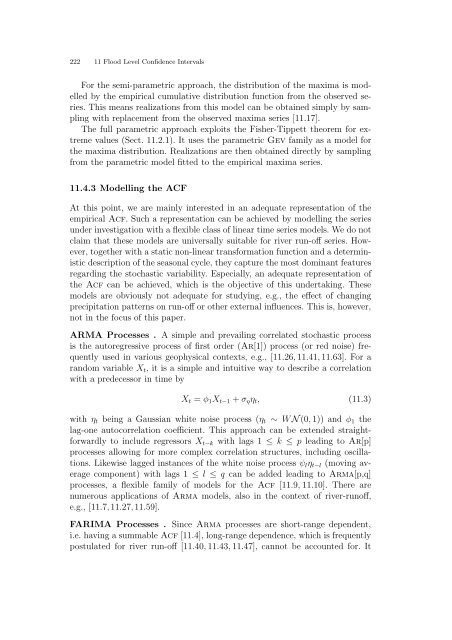
222 11 Flood Level Confidence IntervalsFor the semi-parametric approach, the distribution of the maxima is modelledby the empirical cumulative distribution function from the observed series.This means realizations from this model can be obtained simply by samplingwith replacement from the observed maxima series [11.17].The full parametric approach exploits the Fisher-Tippett theorem for extremevalues (Sect. 11.2.1). It uses the parametric Gev family as a model forthe maxima distribution. Realizations are then obtained directly by samplingfrom the parametric model fitted to the empirical maxima series.11.4.3 Modelling the ACFAt this point, we are mainly interested in an adequate representation of theempirical Acf. Such a representation can be achieved by modelling the seriesunder investigation with a flexible class of linear time series models. We do notclaim that these models are universally suitable for river run-off series. However,together with a static non-linear transformation function and a deterministicdescription of the seasonal cycle, they capture the most dominant featuresregarding the stochastic variability. Especially, an adequate representation ofthe Acf can be achieved, which is the objective of this undertaking. Thesemodels are obviously not adequate for studying, e.g., the effect of changingprecipitation patterns on run-off or other external influences. This is, however,not in the focus of this paper.ARMA Processes . A simple and prevailing correlated stochastic processis the autoregressive process of first order (Ar[1]) process (or red noise) frequentlyused in various geophysical contexts, e.g., [11.26,11.41,11.63]. For arandom variable X t , it is a simple and intuitive way to describe a correlationwith a predecessor in time byX t = φ 1 X t−1 + σ η η t , (11.3)with η t being a Gaussian white noise process (η t ∼ W N(0, 1)) and φ 1 thelag-one autocorrelation coefficient. This approach can be extended straightforwardlyto include regressors X t−k with lags 1 ≤ k ≤ p leading to Ar[p]processes allowing for more complex correlation structures, including oscillations.Likewise lagged instances of the white noise process ψ l η t−l (moving averagecomponent) with lags 1 ≤ l ≤ q can be added leading to Arma[p,q]processes, a flexible family of models for the Acf [11.9, 11.10]. There arenumerous applications of Arma models, also in the context of river-runoff,e.g., [11.7,11.27,11.59].FARIMA Processes . Since Arma processes are short-range dependent,i.e. having a summable Acf [11.4], long-range dependence, which is frequentlypostulated for river run-off [11.40, 11.43, 11.47], cannot be accounted for. It
Henning W. Rust et al. 223is thus desirable to use a class of processes able to model this phenomenon.Granger [11.24] and Hosking [11.29] introduced fractional differencing to theconcept of linear stochastic models and therewith extended the Arma familyto fractional autoregressive integrated moving average (Farima) processes. Aconvenient formulation of such a long-range dependent Farima process X t isgiven byΦ(B)(1 − B) d X t = Ψ(B)η t , (11.4)with B denoting the back-shift operator (BX t = X t−1 ), η t ∼ W N(0, σ η ) awhite noise process, and d ∈ R the fractional difference parameter. The latteris related to the Hurst exponent, which is frequently used in hydrology byH = d + 0.5 [11.4]. The autoregressive and moving average components aredescribed by polynomials of order p and qΦ(z) = 1 −p∑q∑φ i z i , Ψ(z) = 1 + ψ j z j , (11.5)i=1j=1respectively. In practice, the fractional difference operator (1 − B) d has to beexpanded in a power series, cf. [11.24]. A Farima[p, d, q] process is stationaryif d < 0.5 and all solutions of Φ(z) = 0 in the complex plane lie outside theunit circle. It exhibits long-range dependence or long-memory for 0 < d < 0.5.Processes with d < 0 are said to possess intermediate memory, in practicethis case is rarely encountered, it is rather a result of ‘over-differencing’ [11.4].Recently, the Farima model class has been used as a stochastic model forriver run-off, e.g., [11.4, 11.33, 11.40, 11.43, 11.44]. Also self-similar processesare sometimes used in this context. The latter provide a simple model class,but are not as flexible as Farima processes and are thus appropriate only insome specific cases. Farima models, however, can be used to model a largerclass of natural processes including self-similar processes. (For a comprehensiveoverview of long-range dependence and Farima processes refer to [11.4,11.46]and references therein.)Parameter Estimation . The model parameters (φ 1 , ..., φ p , d, ψ 1 , ..., ψ q ) areestimated using Whittle’s approximation to the Ml-estimator [11.4]. It operatesin Fourier space – with the spectrum being an equivalent representationof the autocorrelation function [11.48] – and is computationally very efficientdue to the use of the fast Fourier transform. Therefore, the Whittle estimatoris especially useful for long records where exact Mle is not feasible due tocomputational limits.The model orders p and q are a priori unknown and can be determinedusing the Hannan-Quinn Information Criterion Hic which is advocated forFarima processes:HIC = N log ˆσ η 2 + 2c log log N(p + q + 1), (11.6)
Page 2 and 3: 214 11 Flood Level Confidence Inter
Page 19 and 20: Henning W. Rust et al. 231ble size
Page 21 and 22: Henning W. Rust et al. 233Density0.
Page 23 and 24: Henning W. Rust et al. 235Vilsbibur
Page 25 and 26: Henning W. Rust et al. 237uncertain
Page 27 and 28: Henning W. et al. 239√ˆθ j ± z
Page 29: Henning W. et al. 24111.40 M. Lohre

11. Confidence Intervals for Flood Return Level Estimates assuming ...

Create successful ePaper yourself

Delete template?

Save as template?