11. Confidence Intervals for Flood Return Level Estimates assuming ...

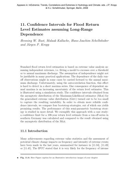
214 11 Flood Level Confidence Intervalsprecipitation to increase [11.32] with increasing global mean temperature. Thisimplies changes in precipitation patterns, a major factor – among some others– for the intensity and frequency of floods, which ultimately can cause tremendousconsequences for nature and societies in a catchment area. This has beenalready observed in many regions of the world [11.37].A pressing question is thus whether heavy rain or severe floods becomemore frequent or intense. Some concepts make use of non-stationary models,e.g., Chapter 5, [11.16, 11.33], or try to identify flood producing circulationpatterns [11.2]. A variety of approaches assess changes by comparing windowscovering different time spans [11.3]. This procedure is especially useful forgetting an impression of possible further developments by comparing GCMcontrol and scenario runs [11.38,11.57]. A useful indicator for changes in floodfrequency and magnitude is the comparison of return level estimates. For thispurpose a reliable quantification of the uncertainty of return level estimates iscrucial.Alerted by an seemingly increasing flood risk, decision makers demand forquantitative and explicit findings for readjusting risk assessment and managementstrategies. Regional vulnerability assessments can be one strategy to dealwith the threat of extremes, such as floods or heat waves (e.g., [11.36]). Otherapproaches try to anticipate extreme scenarios by the help of GCM model runs.The development of risk assessment concepts, however, has still a long way togo, since forecasting of extreme precipitation or floods is highly uncertain (cf.for instance [11.42]). Another potential problem in the risk assessment frameworkis the quantification of uncertainty in extreme value statistics. In situationswhere common statistical approaches might not be applicable as usual,e.g., dependent records, specification of uncertainty bounds for a return levelestimate cannot be made on the basis of the mathematically founded asymptotictheory. The simplified assumption of independent observations usuallyimplies an underestimation of this uncertainty [11.4,11.13,11.35]. The estimationof return levels and their uncertainty plays an important role in hydrologicalengineering and decision making. It forms the basis of setting design valuesfor flood protection buildings like dikes. Since those constructions protect facilitiesof substantial value or are by themselves costly objects, it is certainlyof considerable importance to have appropriate concepts of estimation anduncertainty assessment at hand. Otherwise severe damages, misallocation ofpublic funds, or large claims against insurance companies might be possible.Thus, the approach presented in this contribution focuses on an improvementof common statistical methods used for the estimation of return levels withnon-asymptotic bootstrap method.In the present article, we focus on the block maxima approach and investigatethe maximum-likelihood estimator for return levels of autocorrelatedrun-off records and its uncertainty. In a simulation study, the increase in uncertaintyof a return level estimate due to dependence is illustrated. As a result of

Henning W. Rust et al. 215comparing four strategies based on the bootstrap, we present a concept whichexplicitly takes the autocorrelation into account. It improves the estimation ofconfidence intervals considerably relative to those provided by the asymptotictheory. This strategy is based on a semi-parametric bootstrap approach involvinga model for the autocorrelation function (Acf) and a resampling strategyfrom the maxima series of the observations. The approach is validated usinga simulation study with an autocorrelated process. Its applicability is exemplifiedin a case study: we estimate a 100-year return level and a related 95%upper confidence limit under the different assumptions of independent and dependentobservations. The empirical run-off series was measured at the gaugeVilsbiburg at the river Große Vils in the Danube catchment.The paper is organised as follows: Section 11.2 describes the basic theoryof the block maxima approach of extreme value statistics and the associatedparameter estimation. Section 11.3 illustrates the effect of dependence on thevariability of the return level estimator. In Sect. 11.4 the bootstrap strategiesare presented including the methodological concepts they require. The performanceof the most promising approach is evaluated in Sect. 11.5, followed bya case study in Sect. 11.6. A discussion and conclusions in Sects. 11.7 and 11.8complete the article. Details regarding specific methods used are deferred tothe appendix 11.10.11.2 Basic Theory11.2.1 The Generalised Extreme Value DistributionThe pivotal element in extreme value statistics is the three types theorem, discoveredby Fisher and Tippett [11.22] and later formulated in full generalityby Gnedenko [11.23]. It motivates a family of probability distributions, namelythe general extreme value distributions (Gev), as models for block maximafrom an observed record, e.g., annual maximum discharge. We denote the maximaout of blocks of size n as M n . According to the three types theorem, for nlarge enough the maxima distribution can be approximated byPr{M n ≤ z} ≈ G(z), (11.1)where G(z) is a member of the Gev family (cf. App. 11.10.1).The quality of the approximation in Eq. (11.1) depends in the first placeon the block size n, which in hydrologic applications naturally defaults to oneyear, n = 365. Further influencing factors are the marginal distribution of theobserved series and – a frequently disregarded characteristic – its autocorrelation.Fortunately, the three types theorem holds also for correlated recordsunder certain assumptions (cf. App. 11.10.1). The quality of approximation,however, is affected by the correlation as demonstrated in the following.

216 11 Flood Level Confidence IntervalsWe compare records of white noise and a simple correlated process (Ar[1],cf. Sect. 11.4.3) with the same (Gaussian) marginal distribution. For differentblock sizes n, we extract 2 000 block maxima from a sufficiently long record.Subsequently, the maxima are modelled with a Gumbel distribution being theappropriate limiting distribution in the Gaussian case [11.21]. We measurethe quality of approximation for different n using the negative log-likelihood l(cf. Sect. 11.2.2). Figure 11.1 shows a decreasing negative log-likelihood withincreasing block sizes n for the uncorrelated and the correlated record. This impliesthat the approximation in general ameliorates with block size n. However,neg. Log−Likelihood500 1000 2000White NoiseAR[1]10 20 50 100 500 2000n SizeFig. 11.1. Quality of approximation of a Gumbel fit to 2000 maxima of realizations of a white noiseand an Ar[1] process for different block sizes n. The lines connect the means of 1000 realizations,the shadows mark the mean plus/minus one standard deviation. The vertical line marks a blocksize of n = 365.for all n the approximation is better for the uncorrelated series than for theAr[1] series. This finding is consistent with dependency reducing the effectivenumber of data points [11.62], which in this case translates into a reductionof effective block size. The difference in approximation between the correlatedand the uncorrelated case vanishes with increasing n.11.2.2 GEV Parameter EstimationTo fully specify the model for the extremes, we estimate the Gev parametersfrom the data. Estimates can be obtained in several ways: probability weightedmoments [11.30, 11.31], maximum likelihood (Ml) [11.12, 11.53] or Bayesianmethods [11.12,11.14,11.54]. These different approaches have advantages anddrawbacks which are discussed in e.g., [11.13,11.31] and [11.55]. In the following

Henning W. Rust et al. 217we focus on Ml estimation as the most general method. Within this frameworkmodels can be easily extended, for example to non-stationary distributions[11.34].Let ˆθ = (ˆµ, ˆσ, ˆξ) be the maximum-likelihood estimate (cf. App. 11.10.2) forthe location (µ), scale (σ), and form (ξ) parameter of the Gev. For large blocksizes n approximate (1 − α)100% confidence intervals for these estimates canbe obtained from the Fisher information matrix I E as ˆθ√j ± z α βj,j ; with β2 j,kdenoting the elements of the inverse of I E and z α the (1 − α )-quantile of the2 2standard normal distribution (cf. App. 11.10.2).The m-year return level can be calculated straight forwardly once the location,scale and shape parameter are estimated. In case of the Gumbel distributionthe equation readsˆr m = ˆµ − ˆσ log(y), (11.2)with y = − log(1 − 1 m ). An approximated confidence interval for ˆr m can beobtained using the delta method described in App. 11.10.2 [11.12].For maximum-likelihood estimation of the Gev parameters, we use thepackage evd [11.56] for the open source statistical language environment R[11.50] 1 .11.3 Effects of Dependence on Confidence IntervalsAnnual maxima from river run-off frequently appear uncorrelated from an investigationof the empirical Acf. The left panel in Fig. 11.2 shows the Acfof the annual maxima series from the gauge Vilsbiburg (solid) and of a simulatedrecord (dotted). Both records contain 62 values and their Acf estimatesbasically do not exceed the 95% significance level for white noise. If a longerseries was available, as it is the case for the simulated record, significant autocorrelationof the annual maxima are revealed by the Acf, Fig. 11.2 (right).This implies that considering annual maxima from run-off records a priori asuncorrelated can be misleading.The Ml-estimator relies on the assumption of independent observationsand is thus, strictly speaking, not correct for dependent observations. Themain effect is that standard errors are underestimated if obtained from theFisher information matrix [11.15]. In the following we illustrate this effectby a Monte-Carlo (Mc) simulation study using realizations of a long-range 2dependent process (Far[1,d], cf. Sect. 11.4.3) with Hurst exponent H = 0.75(or, equivalently, fractional differencing parameter d = H − 0.5 = 0.25). Toameliorate resemblance to a daily run-off series, we transform the Gaussian1 Both are freely available from http://cran.r-project.org2 A process is long-range dependent, if its autocorrelation function is not summable, cf. 11.4.3.

218 11 Flood Level Confidence IntervalsACF−0.2 0.2 0.6 1.0VilsbiburgSimulatedACF0.0 0.4 0.80 5 10 15 20Lag[years]length=620 10 20 30 40Lag[years]length=6200Fig. 11.2. Autocorrelation of the empirical maxima series and a section of same length cut outof the simulated series (left). The right panel shows the Acf of the full simulated maxima series(length=6200). The 95% significance levels are marked as dashed lines.series X t with an exponential function. The resulting record Z t = exp(X t ) isthen log-normally distributed.Considering Z t as 100 years of daily run-off (N = 36 500), we perform anextreme value analysis, i.e. we model the annual maxima series by means ofa Gev. Since the marginal distribution is by construction log-normal, we restrictthe extreme value analysis to a Gumbel distribution which is the properlimiting distribution in this case. Exemplarily, a 100-year return level is estimatedusing the Mle (cf. Sect. 11.2.2). Repeating this for 10 000 realizationsof Z t yields a frequency distribution representing the variability of the returnlevel estimator for the Far[1, d] process, shown as histogram in Fig. 11.3 (leftpanel). An analogous simulation experiment has been carried out for an uncorrelatedseries with a log-normal distribution (Fig. 11.3, right panel). Bothhistograms (grey) are compared with the limiting distribution (solid line) ofthe Mle (Eq. (11.19)) evaluated for an ensemble member with return levelestimate close to the ensemble mean. For the uncorrelated series the limitingdistribution provides a reasonable approximation in the sense that it roughlyrecovers the variability of the estimator. In the presence of correlation, the estimatorsvariability is underestimated. This indicates that confidence intervalsderived from the Mle’s limiting distribution are not appropriate here.Alternatively, confidence intervals can be obtained using the profile likelihoodwhich is frequently more accurate [11.12]. Table 11.1 compares the upperlimits of two-sided confidence intervals for three α-levels obtained using profilelikelihood to the limiting distribution and the Monte Carlo simulation. Thelimits from the profile likelihood are indeed for the correlated and the uncorrelatedprocess closer to the limits of the Monte Carlo ensemble. For the

Henning W. Rust et al. 219Correlated seriesUncorrelated seriesDensity0.00 0.10 0.20Density0.00 0.10 0.2030 40 50 60 70 80100−year return levels30 40 50 60 70 80100−year return levelsFig. 11.3. Histogram (grey) of the estimated 100-year return levels from the Mc ensemble of 10000realization of the Far[1, d] process with fractional difference parameter d = 0.25 (or equivalentlyH = 0.75) and Ar parameter φ 1 = 0.9 (left). The right panel shows the result for a white noiseprocess. The realizations contain N = 36500 data points. The solid line shows a Gaussian densityfunction representing the limiting distribution of the 100-year return level estimator derived fromthe Fisher information matrix for one ensemble member.Table 11.1. Upper limits of two-sided confidence intervals for various confidence levels obtainedfrom the asymptotic distribution (Asympt.), the profile likelihood approach (Profile) and the MonteCarlo ensemble (Mc).Uncorrelated SeriesLevel Asympt. Profile Mc0.68 45.97 46.10 46.690.95 48.33 48.90 50.420.99 49.84 50.87 53.10Correlated SeriesLevel Asympt. Profile Mc0.68 52.72 53.00 56.910.95 56.21 57.19 67.260.99 58.43 60.12 75.34correlated process this improvement is not satisfying, since the difference tothe Monte Carlo limit is still about 20% of the estimated return level.To facilitate the presentation in the following, we compare the results fromthe bootstrap approaches to the confidence intervals obtained using the asymptoticdistribution.11.4 Bootstrapping the Estimators VarianceWe discuss non-asymptotic strategies to more reliably assess the variabilityof the return level estimator. These strategies are based on the bootstrap,i.e. the generation of an ensemble of artificial maxima series. These series aresimulated using a model which has been motivated by the data [11.17]. Inthe given setting we estimate the return levels for each ensemble member andstudy the resulting frequency distribution.There are various strategies to generate ensembles. Four of them will bebriefly introduced and, as far as necessary, described in the following.

220 11 Flood Level Confidence Intervalsbootstrap cl . The first approach is a classical bootstrap resampling of themaxima [11.17, 11.19], denoted in the following as bootstrap cl : one ensemblemember is generated by sampling with replacement from the annual maximaseries. Autocorrelation is not taken into account here.iaaft d . We denote the second strategy as iaaft d , it makes use of the dailyobservations. Ensemble members are obtained using the iterative amplitude adjustedFourier transform (Iaaft) – a surrogate method described in Sect. 11.4.4.The Iaaft generates artificial series (so-called surrogates) preserving the distributionand the correlation structure of the observed daily record. Subsequently,we extract the maxima series to obtain an ensemble member. Linearcorrelation is thus accounted for in this case.bootstrap fp . The third strategy is a full parametric bootstrap approach denotedas bootstrap fp . It is based on parametric models for the distribution andthe autocorrelation function of the yearly maxima. This approach operates onthe annual maxima in order to exploit the Fisher-Tippett theorem motivatinga parametric model for the maxima distribution.bootstrap sp . The fourth strategy is a semi-parametric approach, which wecall bootstrap sp . It similarly uses a parametric model for the Acf of the maximaseries, but instead of the Gev we choose a non-parametric model for thedistribution.While the first two strategies are common tools in time series analysis andare well described elsewhere [11.17, 11.52], we focus on describing only thefull-parametric and semi-parametric bootstrap strategy.11.4.1 Motivation of the Central IdeaA return level estimate is derived from an empirical maxima series which canbe regarded as a realization of a stochastic process. The uncertainty of a returnlevel estimate depends on the variability among different realizations of thisprocess. As a measure of this variability, we consider the deviation of a realization’sempirical distribution function from the true distribution function. Ifthis variability is low, it is more likely to have obtained a good representativefor the true maxima distribution from one sample. For a high variability instead,it is harder to get a representative picture of the underlying distributionfrom one sample. We illustrate this effect using long realizations (N = 10 000)from the correlated and the uncorrelated process introduced in Sect. 11.3.We compare the difference between the distributions ˆF s (x) of a short section(N = 100) of a realization and the entire realization’s distribution ˆF 0 (x) bymeans of the Kolmogorov-Smirnov distance D = max x | ˆF s (x) − ˆF 0 (x)| [11.18].Smaller distances D indicate a larger similarity between ˆF s and ˆF 0 . Figure 11.4shows the cumulative distribution function ˆF(D) of these distances D for an

Henning W. Rust et al. 221uncorrelated (circles) and a correlated process (triangles). For the correlatedF(D)0.0 0.4 0.8uncorrelatedcorrelated0.0 0.1 0.2 0.3 0.4DFig. 11.4. Empirical cumulative distribution function ˆF(D) of the Kolmogorov-Smirnov distancesD between sections of a 100 year annual maxima series and the entire 10 000 year annual maximaseries. For the uncorrelated record (○) distances D are located at smaller values than for thecorrelated record (△).process, we find a distribution of distances D located at larger values. Thisimplies that the sections are more diverse in their distribution. Thus for correlatedprocesses the variability in short realization’s maxima distribution islarger than for the uncorrelated process. Realizations of correlated processesare therefore not as likely to yield as representative results for the underlyingdistribution as a comparable sample of an uncorrelated process.Since the variability of the return level estimator is a result of the variabilityof realization’s maxima distribution, we employ this illustrative exampleand study the estimator’s variability among sections of a long record. Ideally,the properties of this long record should be close to the underlying propertiesof the process under consideration. This requires a satisfying model for themaxima series’ distribution and the autocorrelation function. In the approachpursued here, we initially provide two separate models for the two characteristics.Realizations of these two models are then combined to obtain onerealization satisfying both, the desired distribution and the Acf.11.4.2 Modelling the distributionThe aim of modelling the distribution is to provide means for generating realizationsused in a later step of the bootstrap procedure.

222 11 Flood Level Confidence IntervalsFor the semi-parametric approach, the distribution of the maxima is modelledby the empirical cumulative distribution function from the observed series.This means realizations from this model can be obtained simply by samplingwith replacement from the observed maxima series [11.17].The full parametric approach exploits the Fisher-Tippett theorem for extremevalues (Sect. 11.2.1). It uses the parametric Gev family as a model forthe maxima distribution. Realizations are then obtained directly by samplingfrom the parametric model fitted to the empirical maxima series.11.4.3 Modelling the ACFAt this point, we are mainly interested in an adequate representation of theempirical Acf. Such a representation can be achieved by modelling the seriesunder investigation with a flexible class of linear time series models. We do notclaim that these models are universally suitable for river run-off series. However,together with a static non-linear transformation function and a deterministicdescription of the seasonal cycle, they capture the most dominant featuresregarding the stochastic variability. Especially, an adequate representation ofthe Acf can be achieved, which is the objective of this undertaking. Thesemodels are obviously not adequate for studying, e.g., the effect of changingprecipitation patterns on run-off or other external influences. This is, however,not in the focus of this paper.ARMA Processes . A simple and prevailing correlated stochastic processis the autoregressive process of first order (Ar[1]) process (or red noise) frequentlyused in various geophysical contexts, e.g., [11.26,11.41,11.63]. For arandom variable X t , it is a simple and intuitive way to describe a correlationwith a predecessor in time byX t = φ 1 X t−1 + σ η η t , (11.3)with η t being a Gaussian white noise process (η t ∼ W N(0, 1)) and φ 1 thelag-one autocorrelation coefficient. This approach can be extended straightforwardlyto include regressors X t−k with lags 1 ≤ k ≤ p leading to Ar[p]processes allowing for more complex correlation structures, including oscillations.Likewise lagged instances of the white noise process ψ l η t−l (moving averagecomponent) with lags 1 ≤ l ≤ q can be added leading to Arma[p,q]processes, a flexible family of models for the Acf [11.9, 11.10]. There arenumerous applications of Arma models, also in the context of river-runoff,e.g., [11.7,11.27,11.59].FARIMA Processes . Since Arma processes are short-range dependent,i.e. having a summable Acf [11.4], long-range dependence, which is frequentlypostulated for river run-off [11.40, 11.43, 11.47], cannot be accounted for. It

Henning W. Rust et al. 223is thus desirable to use a class of processes able to model this phenomenon.Granger [11.24] and Hosking [11.29] introduced fractional differencing to theconcept of linear stochastic models and therewith extended the Arma familyto fractional autoregressive integrated moving average (Farima) processes. Aconvenient formulation of such a long-range dependent Farima process X t isgiven byΦ(B)(1 − B) d X t = Ψ(B)η t , (11.4)with B denoting the back-shift operator (BX t = X t−1 ), η t ∼ W N(0, σ η ) awhite noise process, and d ∈ R the fractional difference parameter. The latteris related to the Hurst exponent, which is frequently used in hydrology byH = d + 0.5 [11.4]. The autoregressive and moving average components aredescribed by polynomials of order p and qΦ(z) = 1 −p∑q∑φ i z i , Ψ(z) = 1 + ψ j z j , (11.5)i=1j=1respectively. In practice, the fractional difference operator (1 − B) d has to beexpanded in a power series, cf. [11.24]. A Farima[p, d, q] process is stationaryif d < 0.5 and all solutions of Φ(z) = 0 in the complex plane lie outside theunit circle. It exhibits long-range dependence or long-memory for 0 < d < 0.5.Processes with d < 0 are said to possess intermediate memory, in practicethis case is rarely encountered, it is rather a result of ‘over-differencing’ [11.4].Recently, the Farima model class has been used as a stochastic model forriver run-off, e.g., [11.4, 11.33, 11.40, 11.43, 11.44]. Also self-similar processesare sometimes used in this context. The latter provide a simple model class,but are not as flexible as Farima processes and are thus appropriate only insome specific cases. Farima models, however, can be used to model a largerclass of natural processes including self-similar processes. (For a comprehensiveoverview of long-range dependence and Farima processes refer to [11.4,11.46]and references therein.)Parameter Estimation . The model parameters (φ 1 , ..., φ p , d, ψ 1 , ..., ψ q ) areestimated using Whittle’s approximation to the Ml-estimator [11.4]. It operatesin Fourier space – with the spectrum being an equivalent representationof the autocorrelation function [11.48] – and is computationally very efficientdue to the use of the fast Fourier transform. Therefore, the Whittle estimatoris especially useful for long records where exact Mle is not feasible due tocomputational limits.The model orders p and q are a priori unknown and can be determinedusing the Hannan-Quinn Information Criterion Hic which is advocated forFarima processes:HIC = N log ˆσ η 2 + 2c log log N(p + q + 1), (11.6)

224 11 Flood Level Confidence Intervalswith c > 1, ˆσ 2 η the Ml estimate of the variance of the driving noise η t andp + q + 1 being the number of parameters [11.5, 11.6, 11.25]. We choose themodel order p and q such that the Hic takes a minimum.Indirect Modelling of the Maxima Series’ ACF. Modelling the Acf of arun-off maxima series is usually hampered by the shortness of the records. Fora short time series it is often difficult to reject the hypothesis of independence,cf. Sec. 11.3. To circumvent this problem, we model the daily series and assumethat the resulting process adequately represents the daily series’ Acf. It is usedto generate long records whose extracted maxima series are again modelledwith a Farima[p, d, q] process. These models are then considered as adequaterepresentatives of the empirical maxima series Acf. This indirect approach ofmodelling the maxima series’ Acf relies on the strong assumption that themodel for the daily series and also it’s extrapolation to larger time scales isadequate.Modelling a Seasonal Cycle . The seasonal cycle found in a daily riverrun-off series has a fixed periodicity of one year. It can be modelled as a deterministiccycle C(t) which is periodic with period T (1 year): C(t + T) = C(t).Combined with the stochastic model X(t) this yields the following description:Y (t) = C(t) + X(t). (11.7)In the investigated case studies C(t) is estimated by the average yearly cycleobtained by averaging the run-off Q(t) of a specific day over all M years, i.e.Ĉ(t) = 1/M ∑ jQ(t + jT), t ∈ [1, T], cf. [11.28].Including a Static Non-Linear Transformation Function. River runoffis a strictly positive quantity and the marginal distribution is in generalpositively skewed. This suggests to include an appropriate static non-lineartransformation function in the model. Let Z = T(Y ) denote the Box-Coxtransformation (cf. 11.10.3, [11.8]) of the random variable Y (Eq. 11.7). ThenZ is a positively skewed and strictly positive variable, suitable to model riverrun-off. One can think of this static transformation function as a change ofthe scale of measurement. This transformation has been suggested for themodelling of river run-off by Hipel and McLeod [11.28].The full model for the Acf can be written asΦ(B)(1 − B) d X t = Ψ(B)η t (11.8)Y (t) = C(t) + X(t) (11.9)Z(t) = T(Y ). (11.10)Simulation of FARIMA Processes. Several algorithms are known to simulatedata from a Farima process (for an overview refer to [11.1]). Here, we usea method based on the inverse Fourier transform described in [11.60]. It was

Henning W. Rust et al. 225originally proposed for simulating self-similar processes but can be straightforwardlyextended to Farima processes. 311.4.4 Combining Distribution and AutocorrelationHaving a model for the distribution and for the Acf we can generate realizations,i.e. a sample {W i } i=1,...,N from the distribution model and a series{Z i } i=1,...,N from the Farima model including the Box-Cox transformationand, if appropriate, the seasonal cycle. To obtain a time series {Q i } i=1,...,Nwith distribution equal to the one of {W i } i=1,...,N and Acf comparable to thatof {Z i } i=1,...,N , we employ the iterative amplitude adjusted Fourier transform(Iaaft).The Iaaft was developed by Schreiber and Schmitz [11.51] to generatesurrogate time series used in tests for nonlinearity [11.58]. The surrogates aregenerated such that they retain the linear part of the dynamics of the originaltime series including a possible non-linear static transfer function. This impliesthat the power spectrum (or Acf, equivalently) and the frequency distributionof values are conserved. The algorithm basically changes the order of theelements of a record in a way that the periodogram stays close to a desiredone [11.52].Besides using the Iaaft on the daily series to generate an ensemble of surrogates(denoted as iaaft d ), we employ this algorithm also to create records{Q i } i=1,...,N with a periodogram prescribed by a series {Z i } i=1,...,N and a frequencydistribution coming from {W i } i=1,...,N .11.4.5 Generating Bootstrap EnsemblesWith the described methods we are now able to build a model for the distributionand Acf of empirical maxima series and combine them to obtain longrecords. This provides the basis of the full parametric bootstrap ensemblesbootstrap fp and the semi-parametric ensemble bootstrap sp .In detail, the strategies to obtain the ensembles bootstrap fp and bootstrap spcan be outlined as follows:1. Model the correlation structure of the maximaa) If necessary, transform the daily run-off data to follow approximatelya Gaussian distribution using a log or Box-Cox transform [11.8,11.28],cf. 11.10.3.b) Remove periodic cycles (e.g., annual, weekly).3 An R package with the algorithms for the Farima parameter estimation (based on the code fromBeran [11.4]), the model selection (Hic) and the simulation algorithm can be obtained from theauthor.

226 11 Flood Level Confidence Intervalsc) Model the correlation structure using a Farima[p, d, q] process, selectthe model orders p and q with Hic (Sect. 11.4.3).d) Generate a long series from this model (N long 100N data ).e) Add the periodic cycles from 1a). The result is a long series sharing thespectral characteristics, especially the seasonality with the empiricalrecord.f) Extract the annual maxima series.g) Model the correlation structure of the simulated maxima series using aFarima[p max , d, q max ] process, with orders p max and q max selected withHic.2. Model the distribution of the maxima according to the approach usedbootstrap fp : Estimate the parameters of a Gev model from the empiricalmaxima series using Mle (Sect. 11.2.2).bootstrap sp : Use the empirical maxima distribution as model.3. Generate an ensemble of size N ensemble of maxima series with length N maxwith correlation structure and value distribution from the models built in1 and 2:a) Generate a series {Z i } with the Farima[p max , d, q max ] model from step1f) of length N ensemble N max back-transform according to 1a) 4 .b) Generate a sample {W i } with length N ensemble N maxbootstrap fp from the Gev model specified in step 2a).bootstrap sp from sampling with replacement from the empirical maximaseries.c) By means of Iaaft {W i } is reordered such that its correlation structureis similar to that of {Z i }. This yields the run-off surrogates{Q i } i=1,...,Nensemble N max.d) Splitting {Q i } i=1,...,Nensemble N maxinto blocks of size N max yields the desiredensemble.Estimating the desired return level from each ensemble member as describedin Sect. 11.2.2 yields a frequency distribution of return level estimates whichcan be used to assess the variability of this estimator.11.5 Comparison of the Bootstrap ApproachesA comparison of the four different bootstrap approaches bootstrap cl , iaaft d ,bootstrap fp , and bootstrap sp , is carried out on the basis of a simulation study.We start with a realization of a known process, chosen such that its correlationstructure as well as its value distribution are plausible in the context of river4 Instead of back-transforming here, one can Box-Cox transform the outcome of step 3b) combinethe results with Iaaft as in step 3c) and back-transform afterwards. This procedure turned outto be numerically more stable.

Henning W. Rust et al. 227run-off. Here, this is a Farima process similar to those used in [11.43] witha subsequent exponential transformation to obtain a log-normal distribution.This process is used to generate a Monte Carlo ensemble of simulated dailyseries. For each realization we extract the maxima series and estimate a 100-year return level. We obtain a distribution of 100-year return level estimateswhich represent the estimators variability for this process. In the following, thisdistribution is used as a reference to measure the performance of the bootstrapapproaches. A useful strategy should reproduce the distribution of the returnlevel estimator reasonably well.We now take a representative realization out of this ensemble and considerit as a record, we possibly could have observed. On the basis of this “observed”series. From this record, we generate the four bootstrap ensembles accordingto the approaches presented in Sect. 11.4.5. The resulting four frequency distributionsof the 100-year return level estimates are then compared to thedistribution of the reference ensemble and to the asymptotic distribution ofthe Ml-estimator.11.5.1 Monte Carlo Reference EnsembleWe simulate the series for the reference ensemble with a Farima[1, d, 0] processwith parameters d = 0.25 (or H = 0.75), φ 1 = 0.9, variance σ 2 ≈ 1.35,Gaussian driving noise η, and length N = 36 500 (100 years of daily observations).The skewness typically found for river run-off is achieved by subsequentlytransforming the records to a log-normal distribution. To resemble theprocedure of estimating a 100-year return level we extract the annual maximaand estimate a 0.99 quantile using a Gumbel distribution as parametric model.From an ensemble of 100 000 runs, we obtain a distribution of 100-year returnlevels (0.99 quantiles) serving as a reference for the bootstrap procedures.11.5.2 The Bootstrap ensemblesTaking the “observed” series, we generate the four bootstrap ensembles accordingto Sect. 11.4.5. Since iaaft d and bootstrap cl are well described in theliterature, we focus on the semi-parametric and full-parametric approach.Following the outline in Sect. 11.4.5, we start modelling the correlationstructure of the “observed” series using a Farima process as described inSect. 11.4.3. As a transformation, we choose a log-transform as a special caseof the Box-Cox. We treat the process underlying the sample as unknown and fitFarima[p, d, q] models with 0 ≤ q < p ≤ 4. Figure 11.5 shows the result of themodel selection criterion Hic (Eq. (11.6)) for these fits. The Farima[1, d, 0]with parameters and asymptotic standard deviation: d = 0.250 ± 0.008, φ =0.900 ± 0.005, ση 2 = 0.0462 yields the smallest Hic and is chosen to model

228 11 Flood Level Confidence Intervalsthe record. Thus, the proper model structure is recovered and step 1b) iscompleted.[0,0][1,0][1,1][2,0][2,1][2,2][3,0][3,1][3,2][3,3][4,0][4,1][4,2][4,3]HIC2455 2465 2475 2485FARIMA Model Order [p,q]Fig. 11.5. Comparison of the Hic of different Farima[p, d, q] models. Smaller values indicate abetter model. On the abscissa different model orders [p, q] are plotted (0 ≤ q ≤ 3, 0 ≤ p ≤ 4 andq ≤ p). The model orders are discrete, the lines connecting the discrete orders [p, q] are drawn toenhance clarity.With this model we generate an artificial series longer than the originalone (N long = 100N data ) according to step 1c). The extracted annual maximaseries contains N max = 10 000 data points. Since we do not expect theAcf of this maxima series to require a more complex model (in terms ofthe number of parameters) than the daily data, we use orders p ≤ 1 andq = 0, leaving only two models. The Farima[0, d, 0] has a slightly smallerHic value (Hic [0,d,0] =21792.06) than Farima[1, d, 0] (Hic [1,d,0] =21792.40) andwill thus be chosen in the following, step 1f). The resulting parameters ared = 0.205 ± 0.008 and σ 2 η = 0.535.Having modelled the correlation structure we now need a representationfor the distribution. For the full-parametric bootstrap ensemble bootstrap fp ,we get back to the “observed” series and model the annual maxima with aparametric Gumbel distribution, step 2a). This results in Ml-estimates for thelocation and scale parameters: µ = 10.86, σ = 8.35. Since the semi-parametricapproach bootstrap sp does not need a model but uses a classical bootstrapresampling from the empirical annual maxima series, we now can generatethe desired bootstrap ensembles bootstrap fp and bootstrap sp both with 1 000members according to step 3.

Henning W. Rust et al. 229Figure 11.6 compares the frequency distributions of estimated return levelsfrom the four bootstrap ensembles to the reference distribution (grey filled)and to the asymptotic distribution of the Ml-estimator (dotted). The left plotshows the result of the bootstrap cl (solid) and the iaaft d (dashed) ensembles.While bootstrap cl accounts for more variability than the asymptotic distribution,iaaft d exhibits less variability, although it takes autocorrelation of thedaily data into account. This might be due to the fact that the records inthe iaaft d ensemble consists of exactly the same daily run-off values arrangedin a different order. While this allows for some variability on the daily scale,an annual maxima series extracted from such a record is limited to a muchsmaller set of possible values. Since the temporal order of the maxima seriesdoes not influence the return level estimation, the variability of the estimatesis reduced.The right panel in Fig. 11.6 shows the result from the bootstrap sp (solid)and the bootstrap fp (dashed) ensembles. The latter strategy is slightly betterthan the nonparametric bootstrap resampling but still yields a too narrowdistribution. In contrast, the result from the bootstrap sp ensemble gets veryclose to the reference ensemble. Thus, this approach is a promising strategyto improve the uncertainty analysis of return level estimates and is studied inmore detail in the following section.Density0.00 0.04 0.08 0.12Asymptoticbootstrap clDensity0.00 0.04 0.08 0.12Asymptoticbootstrap spbootstrap fpIAAFT d30 40 50 60 70 80 9030 40 50 60 70 80 90100−year return level estimate100−year return level estimateFig. 11.6. Comparison of the result for different bootstrap ensembles to the Mc reference ensemble(grey area) and the asymptotic distribution of the Ml-estimator (dotted). The bootstrap ensemblesconsist each of 1000 members. The left plot shows the results of the nonparametric bootstrapresampling and the daily Iaaft surrogates. The full parametric and semi-parametric bootstrapstrategies are shown in the right plot.

Henning W. Rust et al. 231ble size indicated by the convergence of the grey clouds for each of the fivequantiles. Consequently, the ensemble size should be chosen according to theaccuracy needed. For small sizes, the means of the selected quantiles are closeto the values from the reference ensemble, especially for the three upper quantiles.With an increasing size, difference to the reference ensemble increasesfor the extreme quantiles until they stagnate for ensembles with more thanabout 2000 members. For the 5% and 95% quantiles, the difference betweenthe bootstrap and the Monte Carlo is less than 6% of the return-levels estimate.11.6 Case StudyTo demonstrate the applicability of the suggested semi-parametric bootstrapapproach (bootstrap sp ), we exemplify the strategy with a case study. We considerthe run-off record from the gauge Vilsbiburg at the river Große Vils in theDanube River catchment. Vilsbiburg is located in the south-east of Germanyabout 80km north-east of Munich. The total catchment area of this gauge extendsto 320km 2 . The mean daily run-off has been recorded from 01/11/1939to 07/01/2002 and thus comprises N years = 62 full years or N = 22 714 days.The run-off averaged over the whole observation period is about 2.67 m 3 /s.Extreme Value Analysis . First, we perform an extreme value analysis asdescribed in Sect. 11.2.2, i.e. extracting the annual maxima and determiningthe parameters of a Gev distribution by means of Ml-estimation. In order totest whether the estimated shape parameter ˆξ = 0.04 is significantly differentfrom zero, we compare the result to a Gumbel fit using the likelihood-ratiotest [11.12]. With a p-value of p = 0.74 we cannot reject Gumbel distributionas a suitable model on any reasonable level. The resulting location and scaleparameters with asymptotic standard deviation are µ = (28.5 ± 2.0)m 3 /s andσ = (15.0 ±1.5)m 3 /s. The associated quantile and return level plots are shownin Fig. 11.8 together with their 95% asymptotic confidence limits.According to Eq. (11.2) we calculate a 100-year return level (m = 100) anduse the delta method (11.21) to approximate a standard deviation under thehypothesis of independent observations: r 100 = 97.7 ± 7.9.Modelling the ACF of the Daily Series. In the second step, we modelthe correlation structure which requires preprocessing of the run-off series: Toget closer to a Gaussian distribution, a Box-Cox transformation (sect. 11.10.3)is applied to the daily run-off. The parameter λ = −0.588 is chosen such thatthe unconditional Gaussian likelihood is maximised. Subsequent to this statictransformation, we calculate the average annual cycle in the mean and thevariance, cf. Sect. 11.4.3. The cycle of in the mean is subtracted from therespective days and the result is accordingly divided by the square root of

232 11 Flood Level Confidence IntervalsEmpirical0 50 100 150Return Level0 50 100 15020 40 60 80 100Model0.2 1.0 5.0 20.0 100.0Return PeriodFig. 11.8. Result of the Ml-estimation of the Gumbel parameters for the Vilsbiburg yearly maximaseries compared to the empirical maxima series in a quantile plot (left panel) and return level plot(right panel).the variance cycle. As we find also indication for a weekly component in theperiodogram, we subtract this component analogously. The Box-Cox transformationas well as the seasonal filters have been suggested by Hipel andMcLeod [11.28] for hydrological time series. Although the proposed estimatesof the periodic components in mean and variance are consistent, especially theestimates of the annual cycle exhibits a large variance. Several techniques suchas STL [11.11] are advocated to obtain smoother estimates. Studying thoseperiodic components is, however, not in the focus of this paper.Figure 11.9 shows a comparison of the transformed and mean adjusteddaily run-off record to a Gaussian distribution in form of a density plot (leftpanel) and a plot of empirical versus theoretical quantiles (right panel). Thetransformed distribution is much less skewed than the original one. Differencesto a Gaussian are mainly found in the tails.We now fit Farima[p, d, q] models of various orders with 0 ≤ q ≤ 5, 0 ≤ p ≤6 and q ≤ p and compare the Hic of the different models in Fig. 11.10(left). Thesmallest value for the Hic is obtained for the Farima[3, d, 0] process, which isthus chosen to model the autocorrelation of the daily run-off. The parametersestimated for this process with their asymptotic standard deviation are: d =0.439 ± 0.016, φ 1 = 0.415 ± 0.017, φ 2 = −0.043 ± 0.007, φ 3 = 0.028 ± 0.008and ση 2 = 0.2205. Using the goodness-of-fit test proposed by Beran [11.4], weobtain a p-value of p = 0.015. The model thus cannot be rejected on a 1%level of significance. The result of this fit is shown in the spectral domain inFig. 11.10(right).Modelling the ACF of the Maxima Series. Using this model, a longseries is generated with N long = 100N data . This simulated series is partiallyback-transformed: the overall mean and the seasonal cycles in mean and vari-

Henning W. Rust et al. 233Density0.0 0.2 0.4Sample Quantiles−4 −2 0 2 4−4 −2 0 2 4Quantile−4 −2 0 2 4Theoretical QuantilesFig. 11.9. Comparison of the Box-Cox transformed, deseasonalised and mean adjusted run-offvalues to a Gaussian distribution. Histogram (left, grey) with a density estimate (solid line) andquantile plot (right).HIC30050 30065 30080[0,0][1,0][1,1][2,0][2,1][2,2][3,0][3,1][3,2][4,0][4,1][4,2][4,3][4,4][5,0][5,1][5,2][5,3][6,0][6,1][6,2][6,3][6,5]Spectrum1e−06 1e−02 1e+025e−05 1e−03 5e−02FARIMA Model Order [p,q]Best HIC : FARIMA[3,d,0]FrequencyFARIMA[3,d,0]Fig. 11.10. Model selection for the Box-Cox transformed and deseasonalised daily run-off withmean removed. The spectral density of the model with smallest Hic is shown in double logarithmicrepresentation together with the periodogram (grey) of the empirical series (right panel).ance are added. Note, that the Box-Cox transform is not inverted in this step.From the resulting record, we extract the annual maxima series. Figure 11.2(left panel) shows the Acf of the original maxima series (solid) and comparesit to the Acf of a section of the same length cut out of the maximaseries gained from the simulated run (dotted). The original series has beenBox-Cox transformed as well to achieve a comparable situation. The autocorrelationbasically fluctuates within the 95% significance level (dashed) for awhite noise. However, the full maxima series from the simulated run of 6 200data points exhibits prominent autocorrelation (Fig. 11.2, right panel). Thisindicates that, although an existing autocorrelation structure is not necessarily

234 11 Flood Level Confidence Intervalsvisible in a short sample of a process, it might still be present. Accounting forthis dependence improves the estimation of confidence limits.In the next step, we model the correlation structure of the maxima serieswith a Farima process. Again, we do not expect this series being more adequatelymodelled by a more complex process than the daily data. We use Hicto choose a model among orders p max ≤ p = 3, q max ≤ q = 1. The smallest valuesfor the Hic is attained for a Farima[0, d, 0] model with d = 0.398 ±0.010.The goodness-of-fit yields a p-value of p = 0.319 indicating a suitable model.Combining Distribution and ACF. Having the model for the Acf of themaxima series, we are now able to generate a bootstrap ensemble of artificialdata sets according to the semi-parametric strategy bootstrap sp as described inSect. 11.4.5. We use Iaaft to combine the results of the Farima simulationwith the Box-Cox transformed resampled empirical maxima series. In the laststep the ensemble is restored to the original scale of measurement by invertingthe Box-Cox transform we started with.Calculating the Confidence Limit. Subsequently, the 100-year return levelˆr ∗ (or 0.99 quantile) is estimated for each ensemble member yielding the desireddistribution for the 100-year return level estimator shown in Fig. 11.11.From this distribution we obtain an estimate for a (1 − α)% one-sided upperconfidence limit r α using order statistics. r α is calculated from order statisticsas r α = ˆr 100 − (ˆr(N+1)α ∗ − ˆr 100) [11.17], where the ˆr i ∗ are sorted in ascendingorder. With an ensemble size N ensemble = 9 999 we ensure (N + 1)α being aninteger for common choices of α.To facilitate the comparison of the 95% confidence limits obtained fromthe bootstrap ensemble (rboot 0.95 ≈ 148m3 /s) and the asymptotic distribution(rasymp 0.95 ≈ 110m3 /s) they are marked as vertical lines in Fig. 11.11. The bootstrap95% confidence level rboot 0.95 clearly exceeds the quantile expected fromthe asymptotic distribution confirming the substantial increase in uncertaintydue to dependence. Furthermore, the tails of the bootstrap ensemble decayslower than the tails of the asymptotic distribution. The interpretation of sucha confidence level is the following: In 95% of 100-year return level estimatesthe expected (“true”) 100-year return level will not exceed the 95% confidencelimit.11.7 DiscussionThe approach is presented in the framework of Gev modelling of annual maximausing maximum likelihood. The concept can also be applied in the contextof other models for the maxima distribution (e.g., log-normal) or also differentparameter estimation strategies (e.g., probability weighted moments). Further-

Henning W. Rust et al. 235VilsbiburgDensity0.00 0.01 0.02 0.03 0.04 0.05Asympt.Bootstrap EnsembleAsymptotic DistributionEmpirical Return Level95% QuantilesBootstrap40 60 80 100 120 140 160100−year return levelFig. 11.11. Frequency distribution of the 100-year return level estimates from the bootstrap spensemble with 9 999 members for Vilsbiburg as histogram (grey) and density estimate (solid line)compared to the asymptotic distribution of the Ml estimator derived from the Fisher informationmatrix (dashed). The 100-year return level estimate from the empirical maxima series is marked asdotted vertical line. The 95% quantiles of the asymptotic and bootstrap distributions are indicatedas dashed and solid vertical lines, respectively.more, it is conceivable to extend the class of models describing the dependenceto Farima models with dependent driving noise (Farima-Garch [11.20]) orseasonal models [11.40,11.44].The modelling approach using Farima[p,d,q] models and a subsequent adjustmentof the values has been investigated in more detail by [11.61]. Usingsimulation studies, it was demonstrated that the combination of Farima modelsand the Iaaft is able to reproduce also other characteristics of time seriesthen the distribution and power spectrum. Also the increment distribution andstructure functions for river run-off are reasonably well recovered.In the approach described, we obtain a model for the Acf of the maximaseries only with the help of a model of the daily series. The longer this dailyseries is the more reliable the model will be. Regarding the uncertainty of

236 11 Flood Level Confidence Intervalsreturn level estimates, we might consider this approach with the assumptionof long-range dependence as complementary to the assumption of independentmaxima. The latter assumption yields the smallest uncertainty while, theassumption of long-range dependence yields larger confidence intervals whichcan be considered as an upper limit of uncertainty. The actual detection oflong-range dependence for a given time series is by no means a trivial problem[11.41] but it is not in the focus of this paper.It is also possible to include available annual maxima in the procedure forperiods where daily series have not been recorded. This enhances the knowledgeof the maxima distribution but cannot be used for the modelling of the Acf.11.8 ConclusionWe consider the estimation of return levels from annual maxima series usingthe Gev as a parametric model and maximum likelihood (Ml) parameter estimation.Within this framework, we explicitly account for autocorrelation inthe records which reveals a substantial increase in uncertainty of the floodreturn level estimates. In the standard uncertainty assessment, i.e. the asymptoticconfidence intervals based on the Fisher information matrix or the profilelikelihood, autocorrelations are not accounted for. For long-range dependentprocesses, this results in uncertainty limits being too small to reflect the actualvariability of the estimator. On the way to fill this gap, we study and comparefour bootstrap strategies for the estimation of confidence intervals in the caseof correlated data. This semi-parametric bootstrap strategy outperforms thethree other approaches. It showed promising results in the validation studyusing an exponentially transformed Farima[1,d,0] process. The main idea involvesa resampling approach for the annual maxima and a parametric model(Farima) for their autocorrelation function. The combination of the resamplingand the Farima model is realized with the iterative amplitude adjustedFourier transform, a resampling method used in nonlinearity testing. The resultsof the semi-parametric bootstrap approach are substantially better thanthose based on the standard asymptotic approximation for Mle using theFisher information matrix. Thus this approach might be of considerable valuefor flood risk assessment of water management authorities to avoid floods ormisallocation of public funds. Furthermore, we expect the approach to be applicablealso in other sectors where an extreme value analysis with dependentextremes has to be carried out.The practicability is illustrated for the gauge Vilsbiburg at the River Vilsin the Danube catchment in southern Germany. We derived a 95% confidencelimit for the 100-year flood return level. This limit is about 38% larger thanthe one derived from the asymptotic distribution, a dimension worth beingconsidered for planing options. To investigate to what extend this increase in

Henning W. Rust et al. 237uncertainty depend on catchment characteristics, we plan to systematicallystudy other gauges. Furthermore, a refined model selection strategy and theaccounting for instationarities due to climate change is subject of further work.11.9 AcknowledgementsThis work was supported by the German Federal Ministry of Education andResearch (grant number 03330271) and the European Union Baltic Sea IN-TERREG III B neighbourhood program (ASTRA, grant number 0085). Weare grateful to the Bavarian Authority for the Environment for the provisionof data. We further wish to thank Dr. V. Venema, Dr. Boris Orlowsky, Dr.Douglas Maraun, Dr. P. Braun, Dr. J. Neumann and H. Weber for severalfruitful discussions.11.10 Appendix11.10.1 General Extreme Value DistributionConsider the maximumM n = max{X 1 , . . .,X n } (11.11)of a sequence of n independent and identically distributed (iid) variablesX 1 , . . .,X n with common distribution function F. This can be, for example,daily measured run-off at a gauge; M n then represents the maximum over ndaily measurements, e.g., the annual maximum for n = 365. The three typestheorem states thatPr{(M n − b n )/a n ≤ z} → G(z), as n → ∞, (11.12)with a n and b n being normalisation constants and G(z) a non-degenerate distributionfunction known as the General Extreme Value distribution (Gev){ [ ( )] } −1/ξ z − µG(z) = exp − 1 + ξ. (11.13)σz is defined on {z|1+ξ(z −µ)/σ > 0}. The model has a location parameter µ,a scale parameter σ and a form parameter ξ. The latter decides whether thedistribution is of type II (Fréchet, ξ > 0) or of type III (Weibull, ξ < 0). Thetype I or Gumbel familyG(z) = exp[− exp{−( z − µσ)}], {z| − ∞ < z < ∞} (11.14)

238 11 Flood Level Confidence Intervalsis obtained in the limit ξ → 0 [11.12].It is convenient to transform Eq. (11.12) intoPr{M n ≤ z} ≈ G((z − b n )/a n ) = G ∗ (z). (11.15)The resulting distribution G ∗ (z) is also a member of the Gev family and allowsthe normalisation constants and the location, scale and shape parameter to beestimated simultaneously.We consider an autocorrelated stationary series {X 1 , X 2 , . . .} and define acondition of near-independence: For all i 1 < . . . < i p < j 1 < . . . < j q withj 1 − i p > l,|Pr{X i1 ≤ u n , . . ., X ip ≤ u n , X j1 ≤ u n , . . .,X jq ≤ u n } −(11.16)Pr{X i1 ≤ u n , . . .,X ip ≤ u n }Pr{X j1 ≤ u n , . . .,X jq ≤ u n }| ≤ α(n, l),(11.17)where α(n, l n ) → 0 for some sequence l n , with l n /n → 0 as n → ∞. It canbe shown that the three types theorem holds also for correlated processessatisfying this condition of near-independence [11.12,11.39]. This remarkableresult implies that the limiting distribution of the maxima of uncorrelated and(a wide class) of correlated series belongs to the Gev family.11.10.2 Maximum-Likelihood Parameter Estimation of the GEVLet {M n,1 , M n,2 , . . ., M n,m } be a series of independent block maxima observations,where n denotes the block size and m the number of blocks available forestimation. We denote M n,i as z i . The likelihood function now readsL(µ, σ, ξ) =m∏g(z i ; µ, σ, ξ), (11.18)i=1where g(z) = dG(z)/dz is the probability density function of the Gev. Inthe following, we consider the negative log-likelihood function l(µ, σ, ξ|z i ) =− log L(µ, σ, ξ|z i ).Minimising the log-likelihood with respect to θ = (µ, σ, ξ) leads to the Mlestimate ˆθ = (ˆµ, ˆσ, ˆξ) for the Gev. Under suitable regularity conditions –among them independent observations z i – and in the limit of large block sizes(n → ∞) ˆθ is multivariate normally distributed:ˆθ ∼ MVN d (θ 0 , I E (θ 0 ) −1 ) (11.19)with I E (θ) being the expected information matrix (or Fisher information matrix)measuring the curvature of the log-likelihood. Denoting the elements ofthe inverse of I E evaluated at ˆθ as β j,k we can approximate an (1 − α)100%confidence interval for each component j of ˆθ by

Henning W. et al. 239√ˆθ j ± z α βj,j , (11.20)2with z α being the (1−α/2) quantile of the standard normal distribution [11.12].2The m-year return level can be easily calculated as specified in equation(11.2). An approximated confidence interval for ˆr m can be obtained underthe hypothesis of a normally distributed estimator ˆr m and making use of thestandard deviation σˆrm . The latter can be calculated from the informationmatrix using the delta method [11.12]. For the Gumbel distribution we obtainσ 2ˆr m= β 11 − (β 22 + β 21 ) log(− log(1 − 1 m )) + β 22(log(− log(1 − 1 m )))2 . (11.21)11.10.3 Box-Cox TransformThe Box-Cox transformation can be used to transform a record {x i } such thatits distribution is closer to a Gaussian. For records {x i } with x i > 0 for all i,it is defined as [11.8]{ (x λ −1), λ ≠ 0y = λlog(x), λ = 0We choose the parameter λ such that the unconditional Gaussian likelihoodis maximised. Hipel also advocate the use of this transformation for river runoff[11.28].References11.1 J.-M. Bardet, G. Lang, G. Oppenheim, A. Philippe, and M. S. Taqqu. Generators of longrangedependent processes: A survey. In P. Doukhan, G. Oppenheim, and M. S. Taqqu,editors, Theory and Applications of Long-Range Dependence, pages 579–623. Birkhäuser,Boston, 2003.11.2 A. Bárdossy and F. Filiz. Identification of flood producing atmospheric circulation patterns.Journal of Hydrology, 313(1-2):48–57, 2005.11.3 A. Bárdossy and S. Pakosch. Wahrscheinlichkeiten extremer Hochwasser unter sich änderndenKlimaverhältnissen. Wasserwirtschaft, 7-8:58–62, 2005.11.4 J. Beran. Statistics for Long-Memory Processes. Monographs on Statistics and AppliedProbability. Chapman & Hall, 1994.11.5 J. Beran, R. J. Bhansali, and D. Ocker. On unified model selection for stationary andnonstationary short- and long-memory autoregressive processes. Biometrika, 85(4):921–934,1998.11.6 L. Bisaglia. Model selection for long-memory models. Quaderni di Statistica, 4:33–49, 2002.11.7 P. Bloomfield. Trends in global temperature. Climatic Change, pages 1–16, 1992.11.8 G. E. P. Box and D. R. Cox. An analysis of transformations. J. R. Statist. Soc., 62(2):211–252,1964.11.9 G. E. P. Box and G. M. Jenkins. Time Series Analysis: forecasting and control. PrenticeHall, New Jersey, 1976.11.10 P. J. Brockwell and R. A. Davis. Time series: Theory and Methods. Springer Series inStatistics. Springer, Berlin, 1991.11.11 R.B. Cleveland, W.S. Cleveland, J.E. McRae, and I. Terpenning. Stl: A seasonal-trend decompositionprocedure based on loess. J. Official Statist., 6(1):3–73, 1990.

240 Flood Level Confidence Intervals11.12 S. G. Coles. An Introduction to Statistical Modelling of Extreme Values. Springer, London,2001.11.13 S. G. Coles and M. J. Dixon. Likelihood-based inference for extreme value models. Extremes,2(1):5–23, 1999.11.14 S. G. Coles and J. A. Tawn. A Bayesian analysis of extreme rainfall data. Appl. Stat.,45:463–478, 1996.11.15 S. G. Coles and J. A. Tawn. Statistical methods for extreme values. Internet, 1999.11.16 J. M. Cunderlik and T. B. Ouarda. Regional flood-duration-frequency modeling in the changingenvironment. Journal of Hydrology, 318(1-4):276–291, 2006.11.17 A. C. Davison and D. B. Hinkley. Bootstrap Methods and their Application. Cambridge seriesin Statistical and Probabilistic Mathematics. Cambridge University Press, Cambridge, 1997.11.18 M. H. DeGroot. Probability and Statistics. Series in Statistics. Addison-Wesley, Reading,second edition, 1975.11.19 B. Efron. Bootstrap methods: Another look at the jackknife. Ann. Stat., 7(1):1–26, 1979.11.20 P. Elek and L. Márkus. A long range dependent model with nonlinear innovations for simulatingdaily river flows. Nat. Hazards Earth Syst. Sci., 4:227–283, 2004.11.21 P. Embrechts, C. Klüppelberger, and T. Mikosch. Modelling Extremal Events for Insuranceand Fincance. Springer, Berlin, 1997.11.22 R. A. Fisher and L. H. C. Tippett. Limiting forms of the frequency distribution of the largestor smallest member of a sample. Proc. Cambridge Phil. Soc., 24:180–190, 1928.11.23 B. V. Gnedenko. Sur la distribution limite du terme maximum d’une série aléatoire. Ann.Math. (2), 44:423–453, 1943.11.24 C. W. Granger and R. Joyeux. An introduction to long-memory time series models andfractional differences. J. Time Ser. Anal., 1(1):15–29, 1980.11.25 E. J. Hannan and B. G. Quinn. The determination of the order of an autoregression. J. R.Statist. Soc., 41:190–195, 1979.11.26 H. Held and T. Kleinen. Detection of climate system bifurcations by degenerate fingerprinting.Geophys. Res. Lett., 31(L23207), 2004.11.27 K. W. Hipel and A. I. McLeod. Preservation of the rescales adjusted range 2. Simulationstudies using Box-Jenkins models. Water Resour. Res., 14(3):509–516, 1978.11.28 K.W. Hipel and A.I. McLeod. Time Series Modelling of Water Resources and EnvironmentalSystems. Developement in Water Science. Elsevier, Amsterdam, 1994.11.29 J. R. M. Hosking. Fractional differencing. Biometrika, 68:165–176, 1981.11.30 J. R. M. Hosking. L-moments: analysis and estimation of distributions using linear combinationsof order statistics. J. R. Statist. Soc., B:105–124, 1990.11.31 J. R. M. Hosking, J. R. Wallis, and E. F. Wood. Estimation of the generalized extreme-valuedistribution by the method of probability-weighted moments. Technometrics, 27(3):251–261,1985.11.32 Climate change 2001: The scientific basis, contribution of working group I to the ThirdAssessment Report, 2001. Intergovernmental Panel on Climate Change (IPCC).11.33 M. Kallache, H. W. Rust, and J. Kropp. Trend assessment: Applications for hydrology andclimate. Nonlin. Proc. Geoph., 2:201–210, 2005.11.34 R. W. Katz, M. B. Parlange, and P. Naveau. Statistics of extremes in hydrology. Advancesin Water Resources, 25:1287–1304, 2002.11.35 D. Koutsoyiannis. Climate change, the Hurst phenomenon, and hydrological statistics. Hydrol.Sci. J., 48(1), 2003.11.36 J. P. Kropp, A. Block, F. Reusswig, K. Zickfeld, and H. J. Schellnhuber. Semiquantitativeassessment of regional climate vulnerability: The North Rhine – Westphalia study. ClimaticChange, 76(3-4):265–290, 2006.11.37 Z. W. Kundzewicz. Is the frequency and intensity of flooding changing in Europe. In W. Kirch,B. Menne, and R. Bertollini, editors, Extreme Weather Events and Public Health Responses.Springer, 2005.11.38 Z.W. Kundzewicz and H.-J. Schellnhuber. Floods in the IPCC TAR perspective. NaturalHazards, 31:111–128, 2004.11.39 M. R. Leadbetter, G. Lindgren, and H. Rootzén. Extremes and related properties of randomsequences and processes. Springer Series in Statistics. Springer, New York, 1983.

Henning W. et al. 24111.40 M. Lohre, P. Sibbertsen, and T. Könnig. Modeling water flow of the Rhine River usingseasonal long memory. Water Resour. Res., 39(5):1132, 2003.11.41 D. Maraun, H. W. Rust, and J. Timmer. Tempting long-memory - on the interpretation ofDFA results. Nonlin. Proc. Geophys., 11:495–503, 2004.11.42 B. Merz and A.H. Thieken. Separating natural and epistemic uncertainty in flood frequencyanalysis. J. Hyd., 309:114–132, 2005.11.43 A. Montanari, R. Rosso, and M. S. Taqqu. Fractionally differenced ARIMA models appliedto hydrologic time series: Identification, estimation and simulation. Water Resour. Res.,33(5):1035, 1997.11.44 A. Montanari, R. Rosso, and M. S. Taqqu. A seasonal fractional ARIMA model applied tothe nile river monthly flows. Water Resour. Res., 36(5):1249–1259, 2000.11.45 P. Naveau, M. Nogaj, C. Ammann, P. Yiou, D. Cooley, and V. Jomelli. Statistical methodsfor the analysis of climate extremes. C.R. Geoscience, 377:1013–1022, 2005.11.46 M. Ooms and J. Doornik. Inference and forecasting for fractional autoregressive integratedmoving average models, with an application to us and uk inflation. Technical report,Econometric Institute, Erasmus University, Rotterdam, 1999. Econometric Institute Report9947/A.11.47 M. Ooms and P.H. Franses. A seasonal periodic long memory model for monthly river flows.Environ. Model. & Software, 16:559–569, 2001.11.48 M. B. Priestley. Spectral Analysis and Time Series. Academic Press, London, 1992.11.49 C. Prudhomme, D. Jakob, and C. Svensson. Uncertainty and climate change impact on theflood regime of small UK catchments. J. Hyd., 277:1–23, 2003.11.50 R Development Core Team. R: A language and environment for statistical computing. RFoundation for Statistical Computing, Vienna, Austria, 2004. ISBN 3-900051-07-0.11.51 T. Schreiber and A. Schmitz. Improved surrogate data for nonlinearity tests. Phys. Rev.Lett., 77:635, 1996.11.52 T. Schreiber and A. Schmitz. Surrogate time series. Physica D, 142:346–382, 2000.11.53 R. L. Smith. Maximum likelihood estimation in a class of nonregular cases. Biometrika,72(1):67–90, 1985.11.54 R. L. Smith. Comparison of maximum likelihood and Bayesian estimators for the threeparameterWeibull distribution. Appl.Stat., 36(3):358–369, 1987.11.55 R. L. Smith. Environmental statistics. Internet, 2001. Version 5.0.11.56 A. Stephenson and C. Ferro. evd: Functions for extreme value distributions, 2004. R packageversion 2.1-6.11.57 P. A. Stott, D. A. Stone, and M. R. Allen. Human contribution to the European heatwaveof 2003. Nature, 432, 2004.11.58 J. Theiler, S. Eubank, A. Longtin, B. Galdrikian, and J. D. Farmer. Testing for nonlinearityin time series: The method of surrogate data. Physica D, 58(77), 1992.11.59 J. Timmer. Modeling noisy time series: Physiological tremor. Int. J. Bif. Chaos, 8(7), 1998.11.60 J. Timmer and M. König. On generating power law noise. A&A, 300(3):707–710, 1995.11.61 V. Venema, S. Bachner, H. W. Rust, and C. Simmer. Statistical characteristics of surrogatedata based on geophysical measurements. Nonlin. Proc. Geophys., pages 449–466, 2006.11.62 H. von Storch and F. W. Zwiers. Statistical Analysis in Climate Research. CambridgeUniversity Press, Cambridge ; New York, 1999.11.63 T. M. L. Wigley and P. D. Jones. Detecting CO2-induced climatic change. Nature, 292:205– 208, 1981.peer-reviewed by 2 reviewers