11. Confidence Intervals for Flood Return Level Estimates assuming ...

More documents

Recommendations

Info

236 11 Flood Level Confidence Intervalsreturn level estimates, we might consider this approach with the assumptionof long-range dependence as complementary to the assumption of independentmaxima. The latter assumption yields the smallest uncertainty while, theassumption of long-range dependence yields larger confidence intervals whichcan be considered as an upper limit of uncertainty. The actual detection oflong-range dependence for a given time series is by no means a trivial problem[11.41] but it is not in the focus of this paper.It is also possible to include available annual maxima in the procedure forperiods where daily series have not been recorded. This enhances the knowledgeof the maxima distribution but cannot be used for the modelling of the Acf.11.8 ConclusionWe consider the estimation of return levels from annual maxima series usingthe Gev as a parametric model and maximum likelihood (Ml) parameter estimation.Within this framework, we explicitly account for autocorrelation inthe records which reveals a substantial increase in uncertainty of the floodreturn level estimates. In the standard uncertainty assessment, i.e. the asymptoticconfidence intervals based on the Fisher information matrix or the profilelikelihood, autocorrelations are not accounted for. For long-range dependentprocesses, this results in uncertainty limits being too small to reflect the actualvariability of the estimator. On the way to fill this gap, we study and comparefour bootstrap strategies for the estimation of confidence intervals in the caseof correlated data. This semi-parametric bootstrap strategy outperforms thethree other approaches. It showed promising results in the validation studyusing an exponentially transformed Farima[1,d,0] process. The main idea involvesa resampling approach for the annual maxima and a parametric model(Farima) for their autocorrelation function. The combination of the resamplingand the Farima model is realized with the iterative amplitude adjustedFourier transform, a resampling method used in nonlinearity testing. The resultsof the semi-parametric bootstrap approach are substantially better thanthose based on the standard asymptotic approximation for Mle using theFisher information matrix. Thus this approach might be of considerable valuefor flood risk assessment of water management authorities to avoid floods ormisallocation of public funds. Furthermore, we expect the approach to be applicablealso in other sectors where an extreme value analysis with dependentextremes has to be carried out.The practicability is illustrated for the gauge Vilsbiburg at the River Vilsin the Danube catchment in southern Germany. We derived a 95% confidencelimit for the 100-year flood return level. This limit is about 38% larger thanthe one derived from the asymptotic distribution, a dimension worth beingconsidered for planing options. To investigate to what extend this increase in
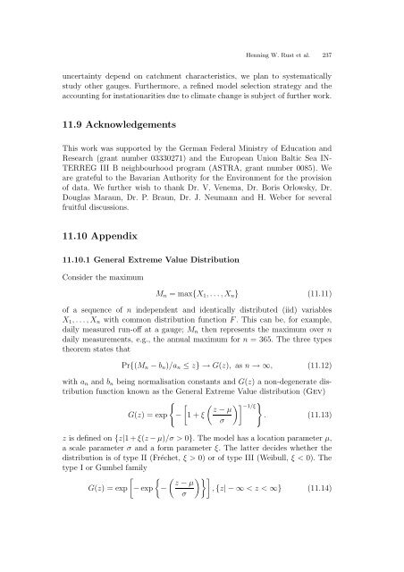
Henning W. Rust et al. 237uncertainty depend on catchment characteristics, we plan to systematicallystudy other gauges. Furthermore, a refined model selection strategy and theaccounting for instationarities due to climate change is subject of further work.11.9 AcknowledgementsThis work was supported by the German Federal Ministry of Education andResearch (grant number 03330271) and the European Union Baltic Sea IN-TERREG III B neighbourhood program (ASTRA, grant number 0085). Weare grateful to the Bavarian Authority for the Environment for the provisionof data. We further wish to thank Dr. V. Venema, Dr. Boris Orlowsky, Dr.Douglas Maraun, Dr. P. Braun, Dr. J. Neumann and H. Weber for severalfruitful discussions.11.10 Appendix11.10.1 General Extreme Value DistributionConsider the maximumM n = max{X 1 , . . .,X n } (11.11)of a sequence of n independent and identically distributed (iid) variablesX 1 , . . .,X n with common distribution function F. This can be, for example,daily measured run-off at a gauge; M n then represents the maximum over ndaily measurements, e.g., the annual maximum for n = 365. The three typestheorem states thatPr{(M n − b n )/a n ≤ z} → G(z), as n → ∞, (11.12)with a n and b n being normalisation constants and G(z) a non-degenerate distributionfunction known as the General Extreme Value distribution (Gev){ [ ( )] } −1/ξ z − µG(z) = exp − 1 + ξ. (11.13)σz is defined on {z|1+ξ(z −µ)/σ > 0}. The model has a location parameter µ,a scale parameter σ and a form parameter ξ. The latter decides whether thedistribution is of type II (Fréchet, ξ > 0) or of type III (Weibull, ξ < 0). Thetype I or Gumbel familyG(z) = exp[− exp{−( z − µσ)}], {z| − ∞ < z < ∞} (11.14)
Page 2 and 3: 214 11 Flood Level Confidence Inter
Page 19 and 20: Henning W. Rust et al. 231ble size
Page 21 and 22: Henning W. Rust et al. 233Density0.
Page 23: Henning W. Rust et al. 235Vilsbibur
Page 27 and 28: Henning W. et al. 239√ˆθ j ± z
Page 29: Henning W. et al. 24111.40 M. Lohre

11. Confidence Intervals for Flood Return Level Estimates assuming ...

Create successful ePaper yourself

Delete template?

Save as template?