Merkle Tree Traversal Techniques - CDC
Merkle Tree Traversal Techniques - CDC
Merkle Tree Traversal Techniques - CDC

Create successful ePaper yourself
Turn your PDF publications into a flip-book with our unique Google optimized e-Paper software.
Darmstadt University of Technology<br />
Department of Computer Science<br />
Cryptography and Computer Algebra<br />
<strong>Merkle</strong> <strong>Tree</strong> <strong>Traversal</strong> <strong>Techniques</strong><br />
Bachelor Thesis<br />
by<br />
Boris Ederov<br />
Prof. Dr. Johannes Buchmann<br />
Supervised by Erik Dahmen<br />
April 2007
Index<br />
Abstract 5<br />
Chapter 1: Introduction 6<br />
Chapter 2: The Basics 8<br />
2.1 Hash and One–Way Functions 8<br />
2.1.1 One - Way Functions 8<br />
2.1.2 Hash functions 9<br />
2.2 Digital Signatures 9<br />
2.2.1 The Definition 9<br />
2.2.2 One - Time Digital Signatures 10<br />
2.3 The Original <strong>Merkle</strong> Digital Signature 10<br />
2.3.1 Introduction 10<br />
2.3.2 The Lamport-Diffie one-time signature scheme 11<br />
2.3.3 Winternitz improvement 12<br />
2.3.4 <strong>Merkle</strong> trees 12<br />
2.3.5 Authentication Paths 13<br />
Chapter 3: <strong>Tree</strong> <strong>Traversal</strong> <strong>Techniques</strong> 14<br />
3.1 Authentication Path Regeneration 14<br />
3.2 Efficient Nodes Computation 14<br />
3.3 The Classic <strong>Traversal</strong> 16<br />
3.3.1 Key Generation and Setup 16<br />
3.3.2 Output and Update 17<br />
3.3.3 Example for the Classic <strong>Traversal</strong> 18<br />
3.4 Fractal <strong>Tree</strong> Representation and <strong>Traversal</strong> 25<br />
3.4.1 Notation 25<br />
3.4.2 Existing and Desired Subtrees 26<br />
3.4.3 Algorithm Presentation 27<br />
3.4.4 Example for the fractal algorithm 29<br />
3
3.5 Logarithmic <strong>Merkle</strong> <strong>Tree</strong> <strong>Traversal</strong> 33<br />
Chapter 4: Algorithm Comparison 35<br />
4.1 The Classic <strong>Traversal</strong> 35<br />
4.2 The Improvement 36<br />
4.3 The Fractal <strong>Traversal</strong> 36<br />
Chapter 5: Conclusions and Future Work 41<br />
Acknowledgements 41<br />
References 42<br />
4
Abstract. We introduce <strong>Merkle</strong> tree traversal techniques. We start with the<br />
original tree traversal and then two improvements. Motivated by the possibility<br />
of using <strong>Merkle</strong> authentication, or digital signatures in slow or space -<br />
constrained environments, RSA Laboratories focused on improving the<br />
efficiency of the authentication/signature operation, building on earlier,<br />
unpublished work of Tom Leighton and Silvio Micali. Although hash<br />
functions are very efficient, too many secret leaf values would need to be<br />
authenticated for each digital signature. By reducing the time or space cost, we<br />
found that for medium - size trees the computational cost can be made<br />
sufficiently efficient for practical use. This reinforced the belief that practical,<br />
secure signature/authentication protocols are realizable, even if the number<br />
theoretic algorithms were not available.<br />
The first published paper, Fractal <strong>Merkle</strong> <strong>Tree</strong> Representation and<br />
<strong>Traversal</strong> [JLMS03], shows how to modify <strong>Merkle</strong>’s scheduling algorithm to<br />
achieve various tradeoffs between storage and computation. The improvement<br />
is achieved by means of a careful choice of what nodes to compute, retain, and<br />
discard at each stage. The use of this technique is “transparent” to a verifier,<br />
who will not need to know how a set of outputs were generated, but only that<br />
they are correct. So the technique can be employed in any construction for<br />
which the generation and output of consecutive leaf pre - images and<br />
corresponding authentication paths is required. The paper was presented at the<br />
Cryptographer’s Track, RSA Conference 2003 (May 2003). This construction<br />
roughly speeds up the signing operation inherent in <strong>Merkle</strong>’s algorithm at a<br />
cost of requiring more space. An implementation of this algorithm is publicly<br />
available.<br />
The second paper, <strong>Merkle</strong> <strong>Tree</strong> <strong>Traversal</strong> in Log Space and Time<br />
[SZY04], exhibits an alternate, basic logarithmic space and time algorithm,<br />
which is very space efficient, but provides no trade off. The improvement over<br />
previous traversal algorithms is achieved as a result of a new approach to<br />
scheduling the node computations. The paper has been presented at Eurocrypt<br />
(May 2004). This construction is roughly as fast as <strong>Merkle</strong>’s original algorithm<br />
[MER79], but requires less space.<br />
Both options increase the options for deployment, even in low - power<br />
or low memory devices.<br />
5
Chapter 1<br />
Introduction<br />
Historically, cryptography arose as a means to enable parties to maintain privacy of the<br />
information they send to each other, even in the presence of an adversary with access to<br />
the communication channel. While providing privacy remains a central goal, the field has<br />
expanded to encompass many others, including not just other goals of communication<br />
security, such as guaranteeing integrity and authenticity of communications and many<br />
more sophisticated and fascinating goals. When you shop on the Internet, for example to<br />
buy a book at Amazon, cryptography is used to ensure privacy of your credit card number<br />
as it travels from you to the shop's server. Or, in electronic banking, cryptography is used<br />
to ensure that your checks cannot be forged. Cryptography has been used almost since<br />
writing was invented. For the larger part of its history, cryptography remained a game of<br />
chess - the good cryptographer must always consider two points of view - of the defender<br />
and the attacker. Although the field retains some of this flavor, the last twenty - five years<br />
have brought in something new. The art of cryptography has now been supplemented<br />
with a legitimate science. Modern cryptography is a remarkable discipline. It is a<br />
cornerstone of computer and communications security, with end products that are<br />
imminently practical. Yet its study touches on branches of mathematics that may have<br />
been considered esoteric, and it brings together fields like number theory, computational -<br />
complexity theory, and probability theory.<br />
The basics that are of great significance for this thesis, we are going to consider in<br />
chapter 2. The most important invention in cryptography comes in 1976 with the<br />
publication of Diffie and Hellman - “New Directions in Cryptography” [DH76]. In it they<br />
introduce the concept of public - key cryptography, a form of cryptography, which<br />
generally allows users to communicate securely without having prior access to a shared<br />
secret key. This is done by using a pair of cryptographic keys, designated as public key<br />
and private key, which are related mathematically. In public key cryptography, the<br />
private key is kept secret, while the public key may be widely distributed. In a sense, one<br />
key "locks" a lock, while the other is required to unlock it. It should not be feasible to<br />
deduce the private key of a pair given the public key, and in high quality algorithms no<br />
such technique is known. One analogy is that of a locked store front door with a mail slot.<br />
The mail slot is exposed and accessible to the public: its location (the street address) is in<br />
essence the public key. Anyone knowing the street address can go to the door and drop a<br />
written message through the slot. However, only the person, who possesses the matching<br />
private key, the storeowner in this case, can open the door and read the message. Every<br />
user can compress a particular message using a process called hashing. From a large<br />
document for example we get a few lines, called message digest (it is not possible change<br />
the message digest back into the original document). If the user encrypts the message<br />
digest with his private key, the result will be the so - called digital signature.<br />
6
Nowadays a very important role in cryptography plays the quantum computer. Integer<br />
factorization is believed to be computationally infeasible with an ordinary computer for<br />
large numbers that are the product of two prime numbers of roughly equal size (e.g.,<br />
products of two 300 - digit primes). By comparison, a quantum computer could solve this<br />
problem relatively easily. If a number has n bits (is n digits long in its binary<br />
representation), then a quantum computer with just over 2n qubits can use some<br />
particular algorithms to find its factors. It can also solve a related problem called the<br />
discrete logarithm problem. This ability would allow a quantum computer to "break"<br />
many of the cryptographic systems in use today, in the sense that there would be a<br />
relatively fast (polynomial time in n) algorithm for solving the problem. In particular,<br />
most of the popular public key ciphers could be much more quickly broken, including<br />
forms of RSA, El - Gamal and Diffie - Hellman. These are used to protect secure Web<br />
pages, encrypted email, and many other types of data. Breaking these would have<br />
significant ramifications for electronic privacy and security. The only way to increase the<br />
security of an algorithm like RSA would be to increase the key size and hope that an<br />
adversary does not have the resources to build and use a powerful enough quantum<br />
computer. It seems plausible that it will always be possible to build classical computers<br />
that have more bits than the number of qubits in the largest quantum computer. If that's<br />
true, then algorithms like RSA could be made secure by ensuring that key lengths exceed<br />
the storage capacities of quantum computers. There are some digital signature schemes<br />
that are believed to be secure against quantum computers. Thus the Lamport - Diffie one<br />
- time digital signature scheme is presented. Roughly speaking, this is a signature<br />
scheme, which is guaranteed to be secure as long as each private key is not used more<br />
than once. It is based on a general hash function.<br />
In 1979 Ralph C. <strong>Merkle</strong> presents in [MER79] a multi - time signature scheme, which<br />
employs a version of the Lamport - Diffie one - time signature scheme. In fact the <strong>Merkle</strong><br />
signature scheme transforms any one - time signature scheme into a multi - time one.<br />
This extension is made by complete binary trees, which we call <strong>Merkle</strong> trees. <strong>Merkle</strong><br />
trees stand as the very basis of this thesis and have found many uses in theoretical<br />
cryptographic constructions. The main role they play is to verify the leaf values with<br />
respect to the publicly known root value and the authentication data of that particular<br />
leaf. This data consists of one node value at each height, where these nodes are the<br />
siblings of the nodes on the path connecting the leaf to the root.<br />
In chapter 3 and 4 we will consider the main problems in this thesis - the <strong>Merkle</strong> tree<br />
traversal problem, algorithms for solving it and their comparison. The <strong>Merkle</strong> tree<br />
traversal is the task of finding efficient algorithms to output the authentication data for<br />
successive leaves. Thus, this purpose is different from other, better - known, tree traversal<br />
problems found in the literature. As elegant as <strong>Merkle</strong> trees are, they are used less than<br />
one might expect. One reason is that known traversal techniques require large amount of<br />
computation, storage or both. This means that only the smallest trees can be practically<br />
used. However, with more efficient traversal techniques, <strong>Merkle</strong> trees may once again<br />
become more compelling, especially given the advantage that cryptographic<br />
constructions based on <strong>Merkle</strong> trees do not require any number theoretic assumptions.<br />
7
Chapter 2<br />
The Basics<br />
In this chapter we are going to introduce the basic mathematical notions in cryptography,<br />
which are of great significance to this thesis. We shall talk briefly about digital signatures<br />
and one - time digital signatures, about hash and one - way functions, and of course,<br />
about the original <strong>Merkle</strong> digital signature, which is of crucial importance for <strong>Merkle</strong> tree<br />
traversal techniques.<br />
2.1 Hash and one - way functions<br />
2.1.1 One - way functions: A one - way function is a mathematical function that is<br />
significantly easier to compute in one direction (the forward direction) than in<br />
the opposite direction (the inverse direction). It might be possible, for example,<br />
to compute the function in the forward direction in seconds but to compute its<br />
inverse could take months or years, if at all possible. A trapdoor one - way<br />
function is a one - way function for which the inverse direction is easy given a<br />
certain piece of information (the trapdoor), but difficult otherwise. Public - key<br />
cryptosystems are based on (presumed) trapdoor one - way functions. The<br />
public key gives information about the particular instance of the function; the<br />
private key gives information about the trapdoor. Whoever knows the trapdoor<br />
can compute the function easily in both directions, but anyone lacking the<br />
trapdoor can only perform the function easily in the forward direction. The<br />
forward direction is used for encryption and signature verification; the inverse<br />
direction is used for decryption and signature generation. In almost all public -<br />
key systems, the size of the key corresponds to the size of the inputs to the one<br />
- way function; the larger the key, the greater the difference between the<br />
efforts necessary to compute the function in the forward and inverse directions<br />
(for someone lacking the trapdoor). For a digital signature to be secure for<br />
years, for example, it is necessary to use a trapdoor one - way function with<br />
inputs large enough that someone without the trapdoor would need many years<br />
to compute the inverse function (that is, to generate a legitimate signature). All<br />
practical public key cryptosystems are based on functions that are believed to<br />
be one - way, but no function has been proven to be so. This means it is<br />
theoretically possible to discover algorithms that can compute the inverse<br />
direction easily without a trapdoor for some of the one - way functions; this<br />
development would render any cryptosystem based on these one - way<br />
functions insecure and useless. On the other hand, further research in<br />
theoretical computer science may result in concrete lower bounds on the<br />
difficulty of inverting certain functions; this would be a landmark event with<br />
significant positive ramifications for cryptography. One way - functions are<br />
basic for this thesis and their major use is for authentication.<br />
8
2.1.2 Hash functions: The term hash apparently comes by way of analogy with its<br />
standard meaning in the physical world, to "chop and mix" [WK01]. The first<br />
use of the concept was in a memo from 1953, some ten years later the term<br />
hash came into use. Mathematically, a hash function (or hash algorithm) is a<br />
method of turning data into a number suitable to be handled by a computer. It<br />
provides a small digital “fingerprint” from any kind of data. The function<br />
substitutes or transposes the data to create that “fingerprint”, usually called<br />
hash value. This value is represented as a short string of random - looking<br />
letters and numbers (for example binary data written in hexadecimal notation).<br />
By hash functions appears also the term hash collision - the situation when two<br />
different inputs produce identical outputs. Of course the better the hash<br />
function, the smaller number of collisions that occur. Similarly in<br />
cryptography we have a cryptographic hash function, which is simply a normal<br />
hash function with additional security properties. This is needed for their use in<br />
various information security applications, such as authentication and message<br />
integrity. Usually a long string of any length is taken as input and a string of<br />
fixed length is given as output. The output is sometimes termed a digital<br />
fingerprint. One desirable property of cryptographic hash functions is collision<br />
resistance. A hash function is collision resistant it is “infeasible” to find a<br />
collision.<br />
It is trivial to prove that every collision resistant hash function is a one - way function.<br />
Because of this we are going to use hash functions instead of one - way ones.<br />
2.2 Digital signatures<br />
2.2.1 The definition: This chapter considers techniques designed to provide the<br />
digital counterpart to a handwritten signature. A digital signature of a message<br />
is a number dependent on some secret known only to the signer, and,<br />
additionally, on the content of the message being signed. Signatures must be<br />
verifiable; if a dispute arises whether a party signed a document (caused by<br />
either a lying signer, trying to repudiate the signature that the party created, or<br />
a fraudulent claimant), an unbiased third party should be able to resolve the<br />
matter equitably, without requiring access to the signer’s secret information<br />
(private key). Digital signatures have many applications in information<br />
security, including authentication, data integrity, and non - repudiation. One of<br />
the most significant applications of digital signatures is the certification of<br />
public keys in large networks. Certification is a means for a trusted third party<br />
(TTP) to bind the identity of a user to a public key, so that at some later time,<br />
other entities can authenticate a public key without assistance from a trusted<br />
third party. The concept and utility of a digital signature was recognized<br />
several years before any practical realization was available. Research has<br />
resulted in many different digital signature techniques. Some offer significant<br />
advantages in terms of functionality and implementation. In more<br />
9
mathematical manner we can give the following definitions, according to<br />
[MOV96]:<br />
1. A digital signature is a data string, which associates a message (in digital<br />
form) with some originating entity.<br />
2. A digital signature generation algorithm is a method for producing a<br />
digital signature.<br />
3. A digital signature verification algorithm is a method for verifying that a<br />
digital signature is authentic (i.e., was indeed created by the specified<br />
entity).<br />
4. A digital signature scheme (or mechanism) consists of signature<br />
generation algorithm and an associated verification algorithm.<br />
5. A digital signature signing process (or procedure) consists of a digital<br />
signature generation algorithm, along with a method for formatting data<br />
into messages, which can be signed.<br />
6. A digital signature verification process (or procedure) consists of a<br />
verification algorithm, along with a method for recovering data from the<br />
message.<br />
2.2.2 One - time digital signatures: One - time digital signature schemes are digital<br />
signature mechanisms, which can be used to sign, at most, one message;<br />
otherwise, signatures can be forged [MOV96]. A new public key is required<br />
for each message that is signed. The public information necessary to verify one<br />
- time signatures is often referred to as validation parameters. When one - time<br />
signatures are combined with techniques for authenticating validation<br />
parameters, multiple signatures are possible. Most, but not all, one - time<br />
digital signature schemes have the advantage that signature generation and<br />
verification are very efficient. One - time digital signature schemes are useful<br />
in applications such as chip cards, where low computational complexity is<br />
required.<br />
2.3 The original <strong>Merkle</strong> digital signature<br />
2.3.1 Introduction: In [MER79] <strong>Merkle</strong> proposed a digital signature scheme that<br />
was based on both one - time signatures and hash functions, and that provides<br />
an infinite tree of one - time signatures. One - time signatures normally require<br />
the publishing of large amounts of data to authenticate many messages, since<br />
each signature can only be used once. <strong>Merkle</strong>'s scheme solves the problem by<br />
implementing the signatures via a tree - like scheme. Every node has a k bit<br />
value and every interior node’s value is a hash function of the node values of<br />
its children. The public key that helps for authentication is placed as root of the<br />
tree. The one - time private keys are used for generation of the leaves and are<br />
authenticated with the help of the root. Although the number of messages that<br />
10
can be signed is limited by the size of the tree, the tree can be made arbitrarily<br />
large.<br />
2.3.2 The Lamport-Diffie one-time signature scheme: In [DH76] Whitfield Diffie<br />
and Martin E. Hellman present a new digital signature, based on hash<br />
functions. Such function Y = f ( X ) is selected. Each user U chooses 2n<br />
random values X0, X1,..., X2n− 1 and computes Y0, Y1,..., Y2n− 1 by Yi = f ( X i)<br />
.<br />
Then U publishes the vector Y = ( Y0, Y1,..., Y2n−1) in a public file under his<br />
name (i.e., in a newspaper or in a public file maintained by a trusted center).<br />
He can publish as many vectors as the number of signatures he is expected to<br />
sign. Now we come to signature generation [EB05]. Alice wants to sign an n -<br />
bit message M to Bob ( M = m0m1... mn−1). She then chooses one of his unused<br />
vectors from the public file and sends it to Bob. Bob verifies the existence of<br />
the vector in the public file. After that Alice and Bob mark the vector as used<br />
in the specific file. Alice computes the signature S= S0S1... Sn−1 by<br />
⎧ X2i, if mi<br />
= 0<br />
Si<br />
= ⎪<br />
⎨<br />
⎪<br />
⎪⎩ X2i+ 1,<br />
if mi<br />
= 1<br />
and sends it to Bob. To verify the signature, Bob computes for all i - s<br />
⎧ Y2i, if mi<br />
= 0<br />
f( Si)<br />
= ⎪<br />
⎨<br />
⎪<br />
⎪⎩ Y2i+ 1,<br />
if mi<br />
= 1<br />
Talking about the security of the signature scheme we claim that if Bob can<br />
invert the hash function f , he can then forge Alice’s signature. Even if he is<br />
given a signature of some message using some vector, he still needs to invert<br />
the hash function f in order to forge a different message using the same<br />
vector. To make this easier to understand we give the following example:<br />
Example: Let X = 01001101 and f ( X ) be a function that just changes 0-s<br />
with 1-s and vice versa. Then Y = 10110010 . Imagine that Alice wants to sign<br />
two messages M 1 = 1010 and M 2 = 1101 with this very same private key X .<br />
Then, according to the definition of the scheme, Alice computes the<br />
corresponding signatures S 1 = 1010 and S 2 = 1011,<br />
and sends them to Bob.<br />
Knowing 1 M , 2 M , 1 S and S 2 it is extremely easy for Bob to forge a new<br />
message M 3 = 1111 with its corresponding signature S 3 = 1011,<br />
just<br />
combining the previous two.<br />
11
2.3.3 Winternitz improvement: One generalization of the Lamport - Diffie<br />
scheme attributed by <strong>Merkle</strong> to Winternitz in [MER79] is to apply the hash<br />
function f to the secret key iteratively a fixed number of times, resulting in<br />
the public key. Briefly the scheme works as follows according to [ECS].<br />
Suppose we wish to sign a n- bit message M . First the message is split into<br />
/<br />
M M M . The secret key is<br />
n t blocks of size t bits. Let these parts be 1, 2 ,..., n/ t<br />
{ ,..., }<br />
sk x x<br />
= o n/ t where i<br />
x is a l - bit value. The public key is<br />
⎜<br />
⎛<br />
2t ⎞<br />
1 ⎟ ⎟nt<br />
/<br />
2t 1 2t 1<br />
( 0) ( 1 ) ... ( nt / )<br />
− ⎧⎪ ⎫<br />
⎪<br />
⎪<br />
− −<br />
= ⎪ ⎪<br />
⎨ � � � ⎪<br />
⎬,<br />
⎪<br />
⎪<br />
⎪⎩ ⎪ ⎪⎭<br />
⎜⎜⎝ ⎠⎟<br />
pk f x f x f x<br />
( )<br />
2<br />
where f ( x) f f ( x)<br />
= is applying f iteratively.<br />
The signature of a message M is computed by considering the integer value of<br />
Int M = I . The signature S is composed of n/ t+ 1 values<br />
the blocks ( )<br />
{ }<br />
0 ,..., n/ t<br />
i i<br />
s s where, for i ≥ 1<br />
2t−− 1 Ii −I<br />
= i ( ) = ( ) , and i i ( )<br />
I<br />
s = f x<br />
s f x f y<br />
i i i<br />
12<br />
∑<br />
0 0<br />
for 1 i n/ t<br />
l n/ t+ 1 . On average, computing a<br />
signature requires 2<br />
t<br />
m<br />
2 evaluations of f . To verify a signature, one splits<br />
t<br />
the message M in n/ t blocks of size t - bits . Let these parts be M1 ,..., M n/ t.<br />
One then verifies that pk is equal to<br />
≤ ≤ . The signature length is ( )<br />
⎧⎪ 2t−− 1 I<br />
i i I1<br />
I ⎫<br />
⎪ ⎪<br />
f /<br />
( s ) ( 1 ) ... n t<br />
⎨ o f s f ( s ⎪<br />
nt / ) ⎬<br />
⎪<br />
⎪⎩ ⎪<br />
⎪⎭<br />
∑ � � � for 1 ≤i≤ n/ t . It is possible<br />
'<br />
to prove that forging a signature of a message M given a message M ,<br />
forging a valid signature S and the public key, requires inversion of the<br />
function f .<br />
2.3.4 <strong>Merkle</strong> trees: The greatest disadvantage of Lamport - Diffie scheme is the<br />
size of the public key. All the verifiers need an authenticated copy of this<br />
public key in order to verify the validity of any signature. In [MER79] <strong>Merkle</strong><br />
proposed the use of binary trees to authenticate a large number of public keys<br />
with a single value, namely the root of the tree. That is how the definition of a<br />
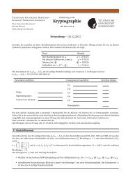
<strong>Merkle</strong> tree comes into use. It is a complete binary tree with a k - bit value<br />
associated to each node such that the interior node value is a hash function of<br />
the node values of its children (Figure 1):
⎡ ( ) ⎤ ⎡ ( ( ) ⎤<br />
⎢ ⎥ ⎢ ⎥ )<br />
Pi ⎡ , j⎤ ⎣ ⎦= f 〈 Pi, i+ j− 1 /2 � P i+ j+ 1 /2, j〉<br />
.<br />
⎣ ⎦ ⎣ ⎦<br />
P is the assignment, which maps the set of nodes to the set of their strings of<br />
length k . In other words, for any interior node n parent and its two child nodes<br />
n left and n right , the assignment P is required to satisfy:<br />
( )<br />
( parent ) = ( nleft<br />
) � ( right )<br />
Pn f P Pn<br />
The N values that need to be authenticated are placed at the N leaves of the<br />
tree. We may choose the leaf value arbitrarily, but usually it is a cryptographic<br />
hash function of the values that need to be authenticated. In this case these<br />
values are called leaf - preimages. A leaf can be verified with respect to a<br />
publicly known root value and its authentication path. We assume that the<br />
public keys of the Lamport - Diffie one- time signature scheme are stored at<br />
the leaf - preimages of the tree (one public key per leaf - preimage).<br />
2.3.5 Authentication paths: Let us set Auth h to be the value of the sibling of the<br />
node of height h on the path from the leaf to the root. Every leaf has height 0<br />
and the hash function of two leaves has height 1, etc. In this manner the root<br />
has height H if the tree has 2 H<br />
= N leaves. Then for every leaf the<br />
authentication path is the set { Authh| 0 ≤ h < H}<br />
. So a leaf can be<br />
authenticated as follows: First we apply our hash function f to the leaf and its<br />
sibling Auth 0 , then we apply f to the result and Auth 1 , and so on all the way<br />
up to the root. If the calculated root value is the same as the published root<br />
value, then the leaf value is accepted as authentic. This operation requires<br />
log2 ( N ) invocations of the hash function f . For detailed information see<br />
[ECS].<br />
Figure 1: <strong>Merkle</strong> tree with 8 leaves. The root can be used to<br />
authenticate the complete tree.<br />
13
Chapter 3<br />
<strong>Tree</strong> traversal techniques<br />
3.1 Authentication path regeneration<br />
As Michael Szydlo mentioned in his paper [SZY04], the main purpose of <strong>Merkle</strong> tree<br />
traversal is to sequentially output the leaf values of all nodes, together with the associated<br />
authentication data. In our third chapter we will discuss three algorithms. First comes the<br />
classic <strong>Merkle</strong> tree traversal algorithm – a straightforward technique which requires a<br />
maximum of 2log2( N ) invocations of the hash function f per round and also a<br />
2<br />
maximum storage of log 2 ( N ) /2 outputs of f . This algorithm is presented for the first<br />
time in 1979 by Ralph <strong>Merkle</strong> [MER79]. The second described algorithm is originally<br />
presented in [JLMS03] and is mainly distinguished because it allows tradeoffs between<br />
time and space. Thus storage can either be minimized or maximized. In the first case the<br />
2log N / log log N invocations of f . In the second -<br />
( )<br />
algorithm requires about 2( ) 2 2(<br />
)<br />
2<br />
1.5log 2( ) / log2( log2(<br />
) )<br />
in [SZY04] and requires 2log2( N ) time and a maximum storage of 2 ( )<br />
N N outputs of f are required. The third algorithm appears first<br />
14<br />
3log N outputs of<br />
f . Some of the described algorithms need a technique to effectively calculating node<br />
values and the root value. These calculations require N − 1 invocations of f , that are not<br />
included in the above mentioned time and storage requirements. They are done by the so<br />
called TREEHASH algorithm, which will be explained in the next paragraph.<br />
3.2 Efficient nodes computation<br />
As already explained, before the application of a traversal technique we need a technique<br />
to quickly pre-calculate a number of node values, together with the root value. This is<br />
done by the TREEHASH algorithm, which is created in a space conserving manner. The<br />
algorithm is really simple. The basic idea is to compute node values at the same height<br />
first, before continuing the calculations with a new leaf, and thus up to the root (keep in<br />
mind that the value ( )<br />
P n of an arbitrary node n of the <strong>Merkle</strong> tree is estimated with the<br />
help of the values of its children nodes). The implementation of TREEHASH is simply<br />
done by a stack (the usage of a stack to simplify the algorithm was influenced by recent<br />
work on time stamping [L02]). At first the stack is empty and then we start adding leaf<br />
values one by one onto it (starting from leaf with index zero). Every round we run a<br />
check if the last two values on the stack are of nodes of the same height or not. In the first<br />
case we calculate the value of the parent node and add it onto the stack, after removing
the two children values first. In the second case we continue adding leaf values until we<br />
reach the first case. The intermediate values stored in the stack during the execution of<br />
the algorithm are called tail node values and create the tail of the stack. This simple<br />
H + 1<br />
implementation is very effective, because for the total of 2 − 1 rounds (one for each<br />
H<br />
node) it requires a maximum of 2 −1computational units for a <strong>Merkle</strong> tree of maximal<br />
height H . In this number are included the calculations of the leaf values which are done<br />
by an oracle LEAFCALC (hash computations and LEAFCALC computations are counted<br />
equally). In the algorithm the leaf indexes are denoted by leaf which is incremented<br />
every round. So LEAFCALC ( leaf ) is simply the value of the leaf with index leaf .<br />
Another important thing about the algorithm is that it stores a maximum of H + 1 hash<br />
values every round, thus conserving space. This is because node values are discarded<br />
when they are not needed any more, which is after their parent value is calculated. Now<br />
we present the algorithm itself:<br />
Algorithm 2.1: TREEHASH (start, maxheight)<br />
1 Set leaf = start and create empty stack.<br />
2 Consolidate: If top 2 nodes on the stack are equal height:<br />
• Pop node value Pn ( right ) from stack.<br />
• Pop node value P( n left ) from stack.<br />
⎛ ⎞<br />
• Compute Pn ( parent ) = f ⎜<br />
⎜Pn ( left) Pn ( right ) ⎟<br />
⎜⎝<br />
⎟<br />
⎠⎟<br />
.<br />
Pn = , output ( parent )<br />
• If height of ( parent ) maxheight<br />
• Push Pn ( parent ) onto the stack and stop.<br />
3 New Leaf: Otherwise:<br />
• Compute Pn ( l ) = LEAFCALC ( leaf ) .<br />
• Push Pn ( l ) onto the stack.<br />
• Increment leaf .<br />
4 Loop to step 2.<br />
15<br />
Pn .<br />
In most cases we need to implement the TREEHASH algorithm into the traversal<br />
algorithms themselves, which means into bigger algorithms. This is possible by defining<br />
an object with two methods. The first method is called initialize and it simply sets which<br />
leaf we start the TREEHASH with, and what the height of the desired output is. For<br />
example later we will meet the following statement - Stackh. initialize( startnode, h )<br />
which tells us that we will modify the Stack h stack starting with the leaf of index<br />
startnode and going up to height h ( h≤ H ). The second method is called update and it
uns either step 2 or step 3 of the TREEHASH algorithm, thus modifying the content of<br />
the used stack (2 and 3 are the steps that actually change the stack). Just to understand<br />
this easier we give another example - Stackh. update ( 2)<br />
. We use the same stack as in the<br />
previous example. It means that for the already known Stack h stack we spend two units<br />
of computation. Which one of the two steps is run depends on the current state of the<br />
stack – if we need to add another leaf value or to calculate a parent node value. After<br />
TREEHASH is run for a particular <strong>Merkle</strong> tree, the only remaining value on the stack is<br />
the value of the root.<br />
3.3 The classic traversal<br />
In [MER79] Ralph <strong>Merkle</strong> presents a new tree traversal technique, that later becomes a<br />
basis for further work and improvements. In a few words only, the algorithm is very<br />
simple. We have our <strong>Merkle</strong> tree, and as usual, the root is the public key and the leaves<br />
are the one-time private keys in our digital signature scheme. By definition, every such<br />
scheme has three phases with the following description:<br />
1. Key generation: In this phase we calculate the root value of the tree, the<br />
first authentication path and some upcoming node values.<br />
2. Output: This phase consists of N rounds, one for each leaf. Every round<br />
the current leaf value is output, together with the authentication path for<br />
this leaf { Auth i}<br />
. After that the tree is updated in order to prepare it for<br />
the next round.<br />
3. Verification: That is the traditional verification of leaf values in a <strong>Merkle</strong><br />
tree. The process is already described in section 2.3.5 and is rather simple.<br />
Now we are going to give a brief explanation of the classic traversal algorithm phase by<br />
phase. The notations that we need are not much – the current authentication nodes are<br />
Auth h . As we need to implement the TREEHASH in our algorithm, we create an object<br />
Stack with a stack of node values. We already explained the two methods initialize and<br />
h<br />
update in the previous section so we have an idea how Stackh. initialize and<br />
Stackh. update are used.<br />
3.3.1 Key Generation and Setup: Let n h, j be the j − th node of height h in our<br />
<strong>Merkle</strong> tree. Thus Auth P( n )<br />
h = h,1<br />
are the values of the very first<br />
authentication path ( h= 0,1,..., H−<br />
1),<br />
which means they are right nodes. The<br />
P n h,0<br />
and they are left nodes.<br />
The algorithm is a direct application of the TREEHASH algorithm, every node<br />
value is computed, but only the described values are stored. In the first step we<br />
upcoming authentication nodes at height h are ( )<br />
16
store the node values included in the authentication path of the first leaf. In the<br />
second step we store P( n h,0)<br />
for every h= 0,1,..., H−<br />
1 and we say Stack h<br />
P n h,0<br />
. In the third step we simply store and output<br />
the root value. Here is the algorithm itself:<br />
contains only the value ( )<br />
Algorithm 3.1: Key Generation and Setup<br />
1 Initial Authentication Nodes: For each h { 0,1,..., H 1}<br />
Calculate Authh P( nh,1)<br />
= .<br />
2 Initial Next Nodes: For each h { 0,1,..., H 1}<br />
with the value of the sibling of h<br />
17<br />
∈ − :<br />
∈ − : Set up Stack h<br />
Auth - ( h,0)<br />
P n (left nodes).<br />
3 Public Key: Calculate and publish tree root value Pn ( root ) .<br />
After this phase of the classic <strong>Merkle</strong> tree traversal we start the next one with<br />
already computed leftmost nodes and their siblings.<br />
3.3.2 Output and Update: This is the phase in which we output every leaf value<br />
together with the authentication path of the corresponding leaf (we use<br />
LEAFCALC for the leaf values computation). For the purpose we have a<br />
counter leaf which starts from zero and is increased by one every round, thus<br />
denoting the index of the current leaf (we run the algorithm once for each leaf<br />
of the tree). The outputs are made in the beginning of every round. After the<br />
output is made we come to the refreshment of the authentication nodes (the<br />
leftmost nodes in the very beginning of the traversal). The idea is that we shift<br />
these authentication nodes to the right when they are no longer needed for<br />
upcoming authentication paths. The authentication node at height h<br />
( h= 0,1,..., H−<br />
1)<br />
needs to be shifted to the right if 2 h divides leaf + 1<br />
without remainder. The new authentication nodes take their values from the<br />
stacks, created in the key generation part. After Auth h is changed, we alter<br />
also the contents of Stackh by using the Stackh. initialize and Stackh. update<br />
methods, thus making further modifications possible. We notice that at round<br />
1 2 h<br />
h h<br />
leaf + + the authentication path will pass through the ( leaf + 1+ 2 ) /2 -<br />
th node at height h . The startnode value of the initialization process (and<br />
future Auth h ) comes from the 2 h leaf values, starting with the leaf with index<br />
( )<br />
h h<br />
leaf + 1+ 2 ⊕ 2 , where ⊕ is a bitwise XOR. Now we present the exact<br />
algorithm:
Algorithm 3.2: Classic <strong>Merkle</strong> <strong>Tree</strong> <strong>Traversal</strong><br />
1 Set leaf = 0<br />
2 Output:<br />
• Compute and output P( nleaf ) = LEAFCALC ( leaf ) .<br />
• For each h∈⎡0, H 1⎤<br />
⎣ − ⎦<br />
output { Auth h}<br />
.<br />
3 Refresh Authentication Nodes:<br />
h<br />
For all h such that 2 leaf + 1:<br />
• Let Auth h become equal to the only node value in Stack h . Empty<br />
the stack.<br />
h h<br />
• Set startnode = ( leaf + 1+ 2 ) ⊕ 2 .<br />
• . ( , )<br />
Stack initialize startnode h .<br />
4 Build Stacks:<br />
For all h∈⎡0, H 1⎤<br />
⎣ − ⎦<br />
:<br />
Stack . update 2<br />
h<br />
• ( )<br />
h<br />
5 Loop:<br />
• Set leaf = leaf + 1.<br />
• If 2 1<br />
H leaf < − go to step 2, otherwise stop.<br />
3.3.3 Example for the classic traversal: To explain more thorough the way this<br />
main algorithm works, we give an example, which follows the algorithm step<br />
3<br />
by step for a <strong>Merkle</strong> tree of maximal height 3 and thus with N = 2 leaves<br />
n0,..., n 7.<br />
First we start with algorithm 3.1, which computes Auth h and puts its<br />
sibling onto Stack h for h ∈ { 0,1,2}<br />
. Thus, in the very beginning<br />
Auth0 = P( n1)<br />
, Auth1= P( n23)<br />
, Auth2 P( n47)<br />
is P( n 0)<br />
, in Stack 1 is P( n 01)<br />
and in Stack 2 is ( 03)<br />
18<br />
Stack<br />
= . The single value in 0<br />
P n . So we start the classic<br />
traversal with some precomputed nodes, which are denoted by grey boxes in<br />
the pictures (see figure 2.1):
Step 1: leaf = 0 .<br />
• ( )<br />
0<br />
Figure 2.1: The tree before the algorithm.<br />
P n with its authentication path { 0, 1, 2}<br />
{ P( n1) , P( n23) , P( n 47)<br />
} are output.<br />
h =<br />
h<br />
is the only solution of 2 / 1 Auth becomes ( )<br />
19<br />
Auth Auth Auth =<br />
• 0<br />
leaf + , so 0 P n 0 ,<br />
because it is the only value in Stack 0 . Stack 0 becomes empty.<br />
3 Stack . initialize 3,0 as described in 3.2.<br />
startnode = so we run 0 ( )<br />
h = we run 0 . Stack update , which only computes ( )<br />
• For 0<br />
onto the stack and stops.<br />
P n , puts it<br />
So the tree after the first round of the algorithm looks like the one in figure 2.2:<br />
Figure 2.2: The tree after round 1.<br />
3
Step 2: leaf = 1.<br />
• ( )<br />
1<br />
P n with its authentication path { 0, 1, 2}<br />
{ P( n0) , P( n23) , P( n 47)<br />
} are output.<br />
h<br />
• 2 / leaf + 1 has two solutions so we consider both cases:<br />
h = 0 :<br />
Auth becomes ( )<br />
• 0<br />
becomes empty. 2<br />
• For h = 0 we run 0 .<br />
onto the stack and stops.<br />
h = 1:<br />
Auth becomes ( )<br />
• 1<br />
20<br />
Auth Auth Auth =<br />
P n 3 , because it is the only value in 0<br />
startnode = so we run Stack0 . initialize ( 2,0)<br />
.<br />
Stack update , which only computes ( )<br />
P n 01 , because it is the only value in 1<br />
Stack . Stack 0<br />
P n , puts it<br />
2<br />
Stack . Stack 1<br />
becomes empty. startnode = 6 so we run Stack1 . initialize ( 6,1)<br />
.<br />
h = we run 1 . Stack update two times. It computes ( 6)<br />
P( n 7)<br />
, puts them onto the stack and stops.<br />
• For 1<br />
So the tree after the second round looks like the one in figure 2.3:<br />
Step 3: leaf = 2 .<br />
• ( )<br />
2<br />
Figure 2.3: The tree after round 2.<br />
P n and<br />
P n with its authentication path { 0, 1, 2}<br />
{ P( n3) , P( n01) , P( n 47)<br />
} are output.<br />
h =<br />
h<br />
is the only solution of 2 / 1 Auth becomes ( )<br />
Auth Auth Auth =<br />
• 0<br />
leaf + , so 0 P n 2 ,<br />
because it is the only value in Stack 0 .<br />
startnode = 5 so we run Stack . initialize ( 5,0)<br />
.<br />
Stack 0 becomes empty.<br />
0
• For h = 0 we run 0 . Stack update , which only computes P( n 5)<br />
, puts it<br />
onto the stack and stops. For h = 1 we run 1 . Stack update , which removes<br />
the previous two values from the stack, computes P( n 67)<br />
and puts it onto<br />
the stack.<br />
So the tree after the third round looks like the one in figure 2.4:<br />
Step 4: leaf = 3.<br />
• ( )<br />
3<br />
Figure 2.4: The tree after round 3.<br />
P n with its authentication path { 0, 1, 2}<br />
{ P( n2) , P( n01) , P( n 47)<br />
} are output.<br />
h<br />
• 2 / leaf + 1 has three solutions so we consider three cases:<br />
21<br />
Auth Auth Auth =<br />
Case 1: h = 0 :<br />
• Auth 0 becomes P( n 5)<br />
, because it is the only value in Stack 0 .<br />
becomes empty. startnode = 4 so we run Stack0 . initialize ( 4,0)<br />
.<br />
Stack 0<br />
• For h = 0 we run 0 . Stack update , which only puts P( n 4)<br />
onto the stack<br />
and then stops.<br />
Case 2: h = 1:<br />
Auth becomes P( n 67)<br />
, because it is the only value in 1<br />
becomes empty. startnode = 4 so we run Stack1 . initialize ( 4,1)<br />
.<br />
h = we run 1 . Stack update two times. First it computes ( 4)<br />
puts it onto the stack, then it puts P( n 5)<br />
onto the stack and stops.<br />
• 1<br />
• For 1<br />
Case 3: h = 2 :<br />
Stack . Stack 1<br />
P n and
P n 03 , because it is the only value in Stack 2 . Stack 2<br />
becomes empty. startnode = 13 , which is too big, so stop.<br />
Auth becomes ( )<br />
• 2<br />
So the tree, after the fourth round, looks like the one in figure 2.5:<br />
Step 5: leaf = 4 .<br />
• ( )<br />
4<br />
Figure 2.5: The tree after round 4.<br />
P n with its authentication path { 0, 1, 2}<br />
{ P( n5) , P( n67) , P( n 03)<br />
} are output.<br />
h =<br />
h<br />
is the only solution of 2 / 1 Auth becomes ( )<br />
22<br />
Auth Auth Auth =<br />
• 0<br />
leaf + , so 0 P n 4 ,<br />
because it is the only value in Stack 0 .<br />
startnode = 7 so we run Stack0 . initialize ( 7,0)<br />
.<br />
Stack 0 becomes empty.<br />
• For h = 0 we run 0 . Stack update , which only puts P( n 7)<br />
onto the stack<br />
and stops. For h = 1 we run 1 . Stack update , which removes the previous<br />
two values from the stack, computes P( n 45)<br />
and puts it onto the stack,<br />
then stops.<br />
So the tree, after the fifth round, looks like the one in figure 2.6:
Step 6: leaf = 5 .<br />
• ( )<br />
5<br />
Figure 2.6: The tree after round 5.<br />
P n with its authentication path { 0, 1, 2}<br />
{ P( n4) , P( n67) , P( n 03)<br />
} are output.<br />
h<br />
• 2 / leaf + 1 has two solutions so we consider both cases:<br />
23<br />
Auth Auth Auth =<br />
Case 1: h = 0 :<br />
• Auth 0 becomes P( n 7)<br />
, because it is the only value in Stack 0 .<br />
becomes empty. startnode = 6 so we run Stack0 . initialize ( 6,0)<br />
.<br />
Stack 0<br />
• For h = 0 we run 0 . Stack update , which only puts P( n 6)<br />
onto the stack<br />
and stops.<br />
Case 2: h = 1:<br />
Auth becomes ( )<br />
• 1<br />
P n 45 , because it is the only value in 1<br />
becomes empty. startnode = 10 , which is too big, so stop.<br />
So the tree, after the sixth round, looks like the one in figure 2.7:<br />
Stack . Stack 1
Step 7: leaf = 6 .<br />
• ( )<br />
6<br />
Figure 2.7: The tree after round 6.<br />
P n with its authentication path { 0, 1, 2}<br />
{ P( n7) , P( n45) , P( n 03)<br />
} are output.<br />
h =<br />
h<br />
is the only solution of 2 / 1 Auth becomes ( )<br />
24<br />
Auth Auth Auth =<br />
• 0<br />
leaf + , so 0 P n 6 ,<br />
because it is the only value in Stack 0 .<br />
startnode = 9 , which is too big, so stop.<br />
Stack 0 becomes empty.<br />
So the tree, after the sixth round, looks like the one in figure 2.8:<br />
Step 8: leaf = 7 .<br />
• ( )<br />
7<br />
Figure 2.8: The tree after round 7.<br />
P n with its authentication path { 0, 1, 2}<br />
{ P( n6) , P( n45) , P( n 03)<br />
} are output.<br />
Auth Auth Auth =
3.4 Fractal tree representation and traversal<br />
In 2003 a group of people introduce a new traversal technique with better space and time<br />
complexity than any other published algorithm [JLMS03]. Most important about it are<br />
two things. The so called fractal traversal is very different from the other two described<br />
techniques in this thesis and has the advantage to allow tradeoffs between storage and<br />
computation (this will be explained more thorough in the comparison chapter after the<br />
algorithm descriptions). We will just mention here that the fractal algorithm requires a<br />
2log N / log log N hash function evaluations for every output (in its<br />
( )<br />
maximum of ( ) ( )<br />
2<br />
worst case) and maximum storage of 1.5log ( ) / log log(<br />
)<br />
25<br />
( )<br />
N N hash values. In this part<br />
we are going to give a brief description of this <strong>Merkle</strong> tree traversal technique, but first<br />
we need to introduce some notations used in it. As usual, we consider a <strong>Merkle</strong> tree T of<br />
height H and 2 H leaves.<br />
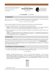
3.4.1 Notations: The basic idea of the fractal algorithm is that it uses subtrees of T<br />
instead of single nodes (like the authentication nodes in the previous<br />
algorithm). That is why we need to choose a fixed height h (1≤h≤H− 1)<br />
and we call it subtree height (for our algorithm we need h to be a divisor of<br />
H ). Let n be an arbitrary node in T . We say that n has altitude h if the<br />
length of the path from n to the nearest leaf is equal to h . For a node n in our<br />
tree we can define an h -subtree at n , which is exactly the subtree that has n<br />
for root and has height h . As h divides H , we can also define L to be the<br />
number of levels of h -subtrees in T (thus L= H / h).<br />
So if the root of a<br />
subtree has altitude ih for some i= 1,2,..., H we say that the subtree is at level<br />
H ih<br />
i (there are 2 − h -subtrees at each level i ). A given series of h -subtrees<br />
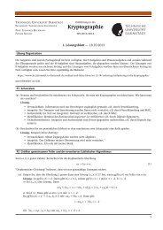
sub<strong>Tree</strong> with j ∈ [ 1,..., L]<br />
is called stacked if the root of sub<strong>Tree</strong> j is a leaf<br />
{ j }<br />
of sub<strong>Tree</strong> j+<br />
1 (see figures 3.1 and 3.2 below).
Figure 3.1: The height of the <strong>Merkle</strong> tree is H . Thus the number of leaves is<br />
2 H<br />
N = . The height of each subtree is h . The altitudes A( t 1)<br />
and A( t 2)<br />
of the<br />
subtrees t 1 and t 2 are marked.<br />
Figure 3.2: Instead of storing all tree nodes, we store a smaller set – those<br />
within the stacked subtrees. The leaf whose pre – image will be output next is<br />
contained in the lowest – most subtree. The entire authentication path is<br />
contained in the stacked set of subtrees.<br />
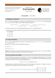
3.4.2 Existing and desired subtrees: In the process of the algorithm we always<br />
have a stacked series of L subtrees, called Exist i . These existing subtrees are<br />
always precomputed, which means that the values of all of their nodes are<br />
already calculated and stored (except of the roots) in the beginning of the<br />
algorithm. Their role in the traversal is very important – they simply contain<br />
the authentication path of every leaf of the lowest subtree Exist 1 (the idea of<br />
the algorithm is that { Exist i}<br />
is constructed and after that modified in order to<br />
26
contain every leaf and its authentication path that have to be output). In the<br />
very beginning of the fractal algorithm the set of existing subtrees is always<br />
the left-most one in T (like on figure 3.3).<br />
Another set of subtrees we are going to need is called the set of desired<br />
subtrees - { Desire i}<br />
, i= 1,2,..., L−<br />
1 (there is no desired subtree at level L ,<br />
because the only possible subtree at this level is an existing subtree). Notice<br />
that this set is not necessary stacked. The positioning of the desired subtrees is<br />
easy to understand – if Exist i (which is already built) has root n k , then the root<br />
of the corresponding desired tree Desire i is n k+<br />
1 (exactly the next node to the<br />
right on the row).<br />
Figure 3.3: The grey subtrees correspond to the existing subtrees, while the<br />
white subtrees correspond to the desired ones. As the existing subtrees are<br />
used up, the desired subtrees are gradually constructed.<br />
The values of the nodes of our desired subtrees need to be calculated and<br />
stored during the algorithm. This, of course, is achieved by using a slightly<br />
modified version of the TREEHASH algorithm, implemented into the main<br />
one. The differences with the original TREEHASH are two. First, the modified<br />
one stops one round earlier, which means that the root of the current Desire i is<br />
not evaluated. Second, the value of every node of height smaller than ih is<br />
saved into Desired i . Now we are going to present the main algorithm itself.<br />
3.4.3 Algorithm presentation: Just like all traversal techniques, the fractal traversal<br />
one has also three phases – key generation, output and verification, which are<br />
precisely the same as the phases of the classic algorithm. An interesting thing<br />
is that the results of the output phase of all described algorithms are the same,<br />
which is the reason not to describe the verification phase.<br />
27
Key Generation and Setup phase:<br />
In this part of the algorithm the set of existing subtrees is defined for a chosen<br />
subtree height h , as already mentioned it consists only of the leftmost h -<br />
subtrees in T . After that the node values of all existing subtrees are<br />
precomputed, except of the roots (meaning that the output phase starts with<br />
already precomputed existing subtrees). A set of desired subtrees is also<br />
created as described in the previous part (the desired subtrees are the right<br />
neighbors of the existing subtrees on the particular level). Every desired<br />
subtree is initialized with an empty stack which makes the use of TREEHASH<br />
possible. We define the starting node of the TREEHASH algorithm for Desire i<br />
to be the leaf with index . 2 ih<br />
Desirei position = ( i= 1,2,..., L−<br />
1).<br />
At the end<br />
the tree root is published. Here is the algorithm step by step:<br />
Algorithm 4.1: Key Generation and Setup<br />
1 Initial Subtrees: For each i∈ { 1,2,..., L}<br />
:<br />
• Calculate all non – root pebbles in existing subtree at level i .<br />
• Create new empty desired subtree at each level i (except for i= L),<br />
with leaf position initialized to 2ih .<br />
2 Public Key: Calculate and publish tree root.<br />
Output and Update Phase:<br />
This part of the algorithm has exactly 2 H<br />
N = rounds, one for each leaf. We<br />
use a counter leaf that denotes the index of the current leaf<br />
( leaf = 0,1,..., N − 1)<br />
and it is regularly increased by one at the end of every<br />
round of the algorithm. In the very beginning of every round the value of the<br />
current leaf together with its authentication path are output. These outputs are<br />
possible because they are part of the already computed nodes of the existing<br />
subtrees.<br />
We say that an existing subtree is no longer useful when it does not contain<br />
future needed authentication paths. In this case that subtree “dies” and the<br />
corresponding desired subtree becomes the new existing one (this means that<br />
by this moment the corresponding desired subtree is fully evaluated to become<br />
existing). The calculated values in the dead subtree are discarded and a new<br />
desired subtree is created to the right of the new existing one. An existing<br />
subtree is shifted to the right (taking the place of the corresponding desired<br />
subtree) only if its desired subtree is completely calculated. After the shift, it<br />
contains the next needed authentication paths. We notice that the existing<br />
subtree at level i (namely Exist i ) is shifted to the right every 2 ih rounds. From<br />
that follows that Desire i should be completed before round 2 ih to be able to<br />
become an existing subtree. This is achieved by applying two units of<br />
28
TREEHASH computation to every desired subtree every round. Here comes the<br />
algorithm itself:<br />
Algorithm 4.2: Fractal <strong>Merkle</strong> <strong>Tree</strong> <strong>Traversal</strong><br />
1 Set leaf = 0 .<br />
2 Output: Authentication path for leaf with index leaf .<br />
3 Next Subtree: For each i for which Exist i is no longer needed, i.e.<br />
hi hi<br />
i∈{ 1,2,..., L−<br />
1}<br />
such that leaf = 2 − 1 ( mod2 ) :<br />
• Remove pebbles in Exist i .<br />
• Rename tree Desire i as tree Exist i .<br />
hi H<br />
• Create new, empty tree Desire i (if leaf + 2 < 2 ).<br />
4 Grow Subtrees: For each i∈{ 1,2,..., L−<br />
1}<br />
: Grow tree Desire i by<br />
applying two units to modified TREEHASH (unless Desire i is<br />
completed) starting from leaf with index 2ih .<br />
H<br />
5 Increment leaf and loop back to step 2 (while leaf < 2 − 1).<br />
3.4.4 Example for the fractal algorithm: To explain more thorough the way this<br />
main algorithm works, we give an example, which follows the algorithm step<br />
3<br />
by step for a <strong>Merkle</strong> tree of maximal height L = 3 and thus with N = 2<br />
leaves n0,..., n 7.<br />
First we start with algorithm 4.1, which computes the nodes of<br />
all existing subtrees and puts creates empty desired subtrees as on the picture.<br />
Thus, in the very beginning Auth0 = P( n1)<br />
, Auth1= P( n23)<br />
, Auth2 = P( n47)<br />
.<br />
Exist 1 consists of 0 n , 1 n and n 01 . Exist 2 consists of n 01 , n 23 and n 03 . The last<br />
existing subtree is Exist 3 and it consists of n 03 , n 47 and the root n 07 . h is<br />
always one, so the height of all subtrees is equal to one. Now we start the<br />
output phase with the precomputed nodes, which are denoted by grey boxes in<br />
the pictures (see figure 4.1):<br />
29
Step 1: leaf = 0 .<br />
• ( )<br />
0<br />
Figure 4.1: The tree before the algorithm.<br />
P n with its authentication path { 0, 1, 2}<br />
{ P( n1) , P( n23) , P( n 47)<br />
} are output.<br />
• Both Exist 1 and 2<br />
30<br />
Auth Auth Auth =<br />
Exist are still needed for future authentication paths, so<br />
we go to the next stage.<br />
• For i = 1,2 we grow the Desire i subtree by applying 2 units of modified<br />
TREEHASH and thus we calculate ( )<br />
2<br />
P( n 4 ) , ( 5 )<br />
P n for Desire 2 .<br />
P n and ( )<br />
Desire and<br />
P n3 for 1<br />
So the tree after the first round of the algorithm looks like the one in figure 4.2:<br />
Step 2: leaf = 1.<br />
Figure 4.2: The tree after round 1.
• ( )<br />
1<br />
P n with its authentication path { 0, 1, 2}<br />
{ P( n0) , P( n23) , P( n 47)<br />
} are output.<br />
31<br />
Auth Auth Auth =<br />
• Exist 1 is no more needed for future authentication paths so we remove all<br />
pebbles in it. 1<br />
Exist becomes Desire 1 and a new empty 1<br />
as denoted on figure 4.3.<br />
• We apply two units of modified TREEHASH to the new Desire 1 and thus<br />
calculate P( n 45 ) , which is now part of it. In 2<br />
and P( n 7 ) .<br />
Desire is created<br />
Desire we calculate P( n )<br />
So the tree after the second round looks like the one in figure 4.3:<br />
Step 3: leaf = 2 .<br />
• ( )<br />
2<br />
Figure 4.3: The tree after round 2.<br />
P n with its authentication path { 0, 1, 2}<br />
{ P( n3) , P( n01) , P( n 47)<br />
} are output.<br />
Auth Auth Auth =<br />
• There is no Exist i which is not needed for future authentication paths to<br />
be output, so we go to the next stage.<br />
• We apply two units of modified TREEHASH to Desire 2 and thus calculate<br />
P( n 67 ) .<br />
So the tree after the third round looks like the one in figure 4.4.<br />
6
Step 4: leaf = 3.<br />
• ( )<br />
3<br />
Figure 4.4: The tree after round 4.<br />
P n with its authentication path { 0, 1, 2}<br />
P( n ) , P( n ) , P( n ) are output.<br />
{ 2 01 47 }<br />
32<br />
Auth Auth Auth =<br />
• Both Exist 1 and Exist2 are not needed for future authentication so we<br />
remove all pebbles in them. Exist 1 becomes Desire 1,<br />
Exist 2 becomes<br />
Desire 2 and a new empty Desire 1 is created as denoted on figure 4.5.<br />
Desire is complete so we make no calculations.<br />
• The new 1<br />
So the tree, after the fourth round, looks like the one in figure 4.5:<br />
Figure 4.5: The tree after round 4.
Step 5: leaf = 4 .<br />
• ( )<br />
4<br />
P n with its authentication path { 0, 1, 2}<br />
{ P( n5) , P( n67) , P( n 03)<br />
} are output.<br />
33<br />
Auth Auth Auth =<br />
• Desire 1 is still needed for future authentication so we do not change the<br />
tree.<br />
Desire is complete so we do not make any calculations.<br />
• 1<br />
So the tree, after the fifth round, remains the same as figure 4.5:<br />
In step 6 we shift Exist 1 for last time and output ( 5 )<br />
path. In steps 7 and 8 we only output P( n 6 ) and ( 7 )<br />
authentication paths.<br />
3.5 Logarithmic <strong>Merkle</strong> <strong>Tree</strong> <strong>Traversal</strong><br />
P n with its authentication<br />
P n together with their<br />
In [SZY04] Michael Szydlo presents an improvement of the classic <strong>Merkle</strong> tree traversal,<br />
called the logarithmic traversal. This improvement differs slightly from the original<br />
<strong>Merkle</strong> algorithm only in the output phase, more particularly, in the part where the stacks<br />
are built and updated. This means that the key generation and verification phases are<br />
absolutely the same as these of the classic traversal. That is why we are going to<br />
concentrate our attention only on the output phase of our new logarithmic algorithm. The<br />
upcoming authentication nodes that have to be output are computed just like in the classic<br />
technique, after that the stacks are initialized normally with a starting node and height.<br />
Now comes the difference in updating the stacks. In the classic algorithm all stacks<br />
receive equal attention, meaning that the same number of computations is spent for each<br />
one of them every step of the algorithm. Because of this, we can consider the updates of<br />
the stacks to be H different TREEHASH processes running in parallel. For large h<br />
values the TREEHASH computations are done a great number of rounds until the stack is<br />
completed, which requires many intermediate nodes to be stored at once. Now the<br />
purpose of the algorithm is to make these computations serially, which in general requires<br />
less space (the main idea is to compute the leftmost stacks first, because they will be<br />
needed for future outputs before the others). That is why in the new technique we want to<br />
complete Stack h for the lowest height h ( h∈[ 0, H−<br />
1]<br />
). If one of the stacks has a lower<br />
tail node than the others, but a bigger height, it is still the first stack to be updated and<br />
grown. To follow this idea we define lmin = min { Stackh. low}<br />
, where Stackh. low denotes<br />
the height of the lowest node in Stack h ( Stackh. low = h if the stack is empty and<br />
Stackh. low =∞ if the stack is complete). If two or more stacks have the same<br />
Stackh. low value, we choose the stack with the smallest index h (which we call focus )<br />
and update it. Thus, after each step of the algorithm, no stacks should contain values of
nodes of height smaller than h (the stacks will then be completed according to the<br />
initializations made earlier in the same round). This is accomplished by applying up to<br />
2H− 1 stack updates every step. Here is the logarithmic algorithm itself:<br />
1<br />
Algorithm 5.1: Logarithmic <strong>Merkle</strong> <strong>Tree</strong> <strong>Traversal</strong><br />
Set leaf = 0<br />
2 Output:<br />
• Compute and output P( n ) = LEAFCALC ( leaf ) .<br />
• For each h ⎡<br />
⎣0, H 1⎤<br />
⎦ Auth h .<br />
3 Refresh Authentication Nodes:<br />
h<br />
For all h such that 2 leaf + 1:<br />
• Let Auth h become equal to the only node value in Stack h .<br />
Empty the stack.<br />
•<br />
h h<br />
Set startnode = ( leaf + 1+ 2 ) ⊕ 2 .<br />
34<br />
leaf<br />
∈ − output { }<br />
• . ( , )<br />
Stack initialize startnode h .<br />
h<br />
4 Build Stacks:<br />
Repeat the following 2H −1<br />
times:<br />
Stack . low .<br />
• Let min<br />
l be the minimum of { h }<br />
Stack . low l .<br />
• Let focus be the least h for which h = min<br />
• . ( 1)<br />
Stack update .<br />
focus<br />
5 Loop:<br />
• Set leaf = leaf + 1.<br />
• If 2H leaf < go to step 2, otherwise stop.<br />
Because of the similarity between the Classic and Logarithmic algorithms we are not<br />
going to consider a special example for the latter.
Chapter 4<br />
Algorithm Comparison<br />
In this part of the thesis we will focus on the similarities and differences between the<br />
already described algorithms. Our main purpose is to consider both time and space<br />
requirements of every traversal technique from the previous chapter and to compare their<br />
efficiency in various situations. The size of the <strong>Merkle</strong> tree and the potentialities of the<br />
computer system we use are of course the main circumstances we need to consider. We<br />
are first going to start our arguments about the classic tree traversal and its improvement<br />
– the logarithmic one. The characteristics of the fractal traversal technique will be given<br />
aside from the other two, because of its totally different idea and structure. At the very<br />
end of this chapter we will give an example of the work of the three algorithms for<br />
<strong>Merkle</strong> trees of fixed sizes. Before we continue with the analysis of the traversals we<br />
should explain that in this chapter by using the term operation we mean elementary<br />
operation such as computation of a leaf value or hash function estimation.<br />
4.1 The classic traversal: As described in the previous chapter, the classic <strong>Merkle</strong><br />
tree traversal is based on the TREEHASH algorithm for more effective<br />
calculation of the tree nodes. For a tree of maximal height H , we run one<br />
instance of TREEHASH for every height h (0≤ h< H ) and thus H different<br />
instances are updated in parallel every round of the algorithm. At height h we<br />
H h 1<br />
have exactly 2 −− right nodes and the same number of left ones. Of course<br />
we use TREEHASH to calculate the values of these nodes, and logically, the<br />
number of needed operations depends on h . For a node of height h the<br />
h+ 1<br />
required number of TREEHASH operations is exactly 2 − 1.<br />
Thus the total<br />
amount of computations needed for a particular height h may be rounded up<br />
H + 1<br />
to 2 = 2N,<br />
which is exactly 2 computations per round (this is the reason<br />
why every TREEHASH instance is updated with two units of computation<br />
every round). If we add together the required operations for all heights h we<br />
will get the total number of required operations per round of the classic<br />
2H = 2log N operations.<br />
algorithm, which is ( )<br />
Talking about the storage requirements of the classic algorithm we make the<br />
following arguments. As already explained, we may have up to H<br />
simultaneously running TREEHASH processes (one for every height h ). For a<br />
given h we observe that the stack at this height may contain up to h+ 1<br />
values. This means that after every round of the algorithm a maximum of<br />
1+ 2 + ... + H values are saved into the stacks. Thus we estimate the space<br />
2 2<br />
complexity of the algorithm to be Ο ( H / 2) =Ο ( log ( N)<br />
/2)<br />
. Imagine that<br />
we are given a big enough <strong>Merkle</strong> tree and we apply the classic traversal to it.<br />
35
The bigger the height of the TREEHASH instance, the greater the number of<br />
saved node values in its stack, which leads us to huge storage requirements and<br />
makes the classic traversal highly inefficient for larger trees.<br />
4.2 The improvement: Years after the original <strong>Merkle</strong> algorithm was created, an<br />
improved version appears. Michael Szydlo realizes that the scheduling strategy<br />
(step four in algorithm 3.2) of the classic traversal is what makes the storage<br />
requirements so big. The improved algorithm that he presents is called<br />
logarithmic traversal (description may be found in part 3.5 of the thesis) and<br />
the way the stacks are modified is changed. The new scheduling strategy<br />
makes up to 2H− 1 updates of a particularly chosen stack and every update is<br />
now done by spending just one unit of TREEHASH computation (instead of<br />
two by the classic traversal). Thus, the number of operations per round remains<br />
the same - proof of this claim can be found in [SZY04]. Now if we analyze the<br />
storage requirements of the new traversal technique, we see that the new stack<br />
update method requires less space, which is its main idea. The number of<br />
Auth i nodes in the <strong>Merkle</strong> tree is always H . If we add the number of already<br />
completed nodes and the number of intermediate node values in the stacks we<br />
get the storage requirements of the algorithm – up to 3H− 2 node values are<br />
saved every round (a detailed proof is in [SZY04]). This results a<br />
Ο 3H =Ο 3log N space complexity, which compared to the<br />
( ) ( ( ) )<br />
2 ( log ( N ) /2)<br />
Ο space complexity of the classic traversal is much better. Thus,<br />
we prefer the usage of the logarithmic traversal for bigger trees. Actually, the<br />
new scheduling strategy of the presented logarithmic algorithm is not the best<br />
one. In an earlier version of his paper [SZY03], Michael Szydlo presented an<br />
algorithm which is even more effective than the described one. In it the left<br />
nodes of the tree are calculated almost for free and this halves the required<br />
hash computations each round. Unfortunately, the algorithm was more<br />
complicated and was not included in the original version of the paper.<br />
4.3 The fractal traversal: We already presented the fractal tree representation and<br />
traversal technique in part 3.4 of the thesis (Algorithm 4.2). It is also an<br />
improvement of the classic traversal, but it has a different strategy. The fractal<br />
scheduling pattern comes from methods for fractal traversal of hash chains<br />
[CJ02], [J02], [S03]. The algorithm itself is simple and is the only one which<br />
allows tradeoffs between storage and computation, depending on the choice of<br />
the parameter h (which, at this point, makes it unique). The time requirements<br />
are easy to estimate – we see that the algorithm in its fourth step applies two<br />
units of TREEHASH computation to every desired subtree. As the maximal<br />
number of desired subtrees is L− 1 (remember that L= H / h),<br />
the maximal<br />
number of operations each round is 2( L− 1) < 2 H / h.<br />
This number of<br />
calculations is considerably smaller that the number of calculations of any<br />
previously described algorithm.<br />
Now we want to estimate the storage requirements of the fractal algorithm. We<br />
need to keep the values of all nodes of both all existing and desired subtrees.<br />
36
We have L existing subtrees in our <strong>Merkle</strong> tree and up to L− 1 desired<br />
h+<br />
1<br />
2L−1 2 − 2 , because<br />
subtrees. For them we need a maximum space of ( )( )<br />
h+ 1<br />
every subtree has 2 − 2 nodes (the root is not included). We also need space<br />
for the intermediate nodes of the TREEHASH stacks, but we have to exclude<br />
those nodes that are part of the desired subtrees themselves. For a desired<br />
subtree with root of height ih (subtree at level i , i > 1)<br />
there are no more than<br />
hi− ( 1) + 1 such nodes in the stack tail. After making the calculations (that<br />
may be found in [JLMS03]) we estimate the maximal space required by the<br />
h+ 1 h+<br />
1 2<br />
algorithm and bound it from above by 2L2 + HL/2= 2H2 / h+ H /2h.<br />
Considering the fractal algorithm, the only problem is that the bigger the<br />
subtree height h is, the faster the algorithm will run, but the more space it will<br />
require. This is exactly the reason why we should find an optimal h to<br />
minimize the storage requirements. We see that for very small h and big tree<br />
2<br />
height H our space requirements are still huge, because H /2h<br />
remains<br />
large. Thus, by differentiation, an optimal value h is found. A better looking<br />
approximation of this value is h= log( H) = loglog(<br />
N)<br />
. For this h the<br />
2<br />
5/ 2log N / loglog N and the number of<br />
storage requirements become ( ) ( )<br />
operations is bounded by 2log ( N) / log log(<br />
N ) . The space requirements may<br />
be reduced even a little more by a slight modification, explained in [JLMS03].<br />
The idea is that actually in almost all cases we may discard intermediate values<br />
of existing subtrees as soon as they have entered the corresponding desired<br />
2<br />
subtree. Thus the space requirements are reduced to 1,5log ( N) / 2loglog(<br />
N ) .<br />
These results improve both time and space requirements of all previously<br />
published traversal techniques, but for bigger <strong>Merkle</strong> trees we still have great<br />
space consumption, which makes the fractal technique more inefficient than<br />
the logarithmic traversals presented by M. Szydlo in 2003 and 2004.<br />
To generalize the explanations made earlier we present a table with the requirements of<br />
all described algorithms from the previous chapter plus the version of Szydlo’s algorithm<br />
from 2003:<br />
The traversals with their space and time requirements:<br />
<strong>Traversal</strong> Technique: Time Requirements: Storage Requirements:<br />
Classic <strong>Merkle</strong> <strong>Traversal</strong><br />
1979<br />
2log( N )<br />
2<br />
log ( N ) /2<br />
Logarithmic <strong>Traversal</strong><br />
2003<br />
log( N )<br />
3log( N )<br />
Logarithmic <strong>Traversal</strong><br />
2004<br />
2log( N )<br />
3log( N )<br />
Fractal <strong>Traversal</strong><br />
2003<br />
2log ( ) / log log(<br />
)<br />
2<br />
1,5log N / 2log log N<br />
N N ( ) ( )<br />
37
To be a little more specific and to investigate the behavior of the four techniques we give<br />
some examples on how they would work in real life, using three exemplary trees. These<br />
<strong>Merkle</strong> trees have different heights and give an idea in which particular situation our<br />
algorithms may be used. Let T i ( i = 1,2,3)<br />
be <strong>Merkle</strong> trees of height H 1 = 5 , H 2 = 10<br />
and H 3 = 20 . The time requirements for these trees (in number of elementary operations)<br />
are given in the following table:<br />
<strong>Traversal</strong><br />
Technique:<br />
Classic <strong>Merkle</strong><br />
<strong>Traversal</strong><br />
1979<br />
Logarithmic<br />
<strong>Traversal</strong><br />
2003<br />
Logarithmic<br />
<strong>Traversal</strong><br />
2004<br />
Fractal<br />
<strong>Traversal</strong><br />
2003<br />
Time requirements in number elementary operations:<br />
Time Requirements<br />
for T 1<br />
10<br />
5<br />
10<br />
4,3068<br />
Time Requirements<br />
for 2 T<br />
38<br />
20<br />
10<br />
20<br />
6,0207<br />
Time Requirements<br />
for 3 T<br />
40<br />
20<br />
40<br />
9,2552<br />
Now we show the space requirements (in number of saved hash values) for the same<br />
<strong>Merkle</strong> trees. More drastic differences may be seen in the following table:<br />
<strong>Traversal</strong><br />
Technique:<br />
Classic <strong>Merkle</strong><br />
<strong>Traversal</strong><br />
1979<br />
Logarithmic<br />
<strong>Traversal</strong><br />
2003<br />
Logarithmic<br />
<strong>Traversal</strong><br />
2004<br />
Fractal<br />
<strong>Traversal</strong><br />
2003<br />
Space requirements in number of saved hash values:<br />
Space Requirements<br />
for T 1<br />
12,5<br />
15<br />
15<br />
8,0753<br />
Space Requirements<br />
for 2 T<br />
50<br />
30<br />
30<br />
22,5774<br />
Space Requirements<br />
for 3 T<br />
200<br />
60<br />
60<br />
69,4139
Talking about space requirements we have to notice the fact that the real space<br />
requirements of all algorithms depend on the output length of our hash function. The next<br />
and last two tables show us the space requirements in bits for hash functions with 160-bit<br />
output and with 256-bit output:<br />
<strong>Traversal</strong><br />
Technique:<br />
Classic <strong>Merkle</strong><br />
<strong>Traversal</strong><br />
1979<br />
Logarithmic<br />
<strong>Traversal</strong><br />
2003<br />
Logarithmic<br />
<strong>Traversal</strong><br />
2004<br />
Fractal<br />
<strong>Traversal</strong><br />
2003<br />
<strong>Traversal</strong><br />
Technique:<br />
Classic <strong>Merkle</strong><br />
<strong>Traversal</strong><br />
1979<br />
Logarithmic<br />
<strong>Traversal</strong><br />
2003<br />
Logarithmic<br />
<strong>Traversal</strong><br />
2004<br />
Fractal<br />
<strong>Traversal</strong><br />
2003<br />
Space requirements for a 160-bit hash function:<br />
Space Requirements<br />
for T 1<br />
2000 bits (0,25kB)<br />
2400 bits (0,3kB)<br />
2400 bits (0,3kB)<br />
1292,048 bits<br />
(0,1615kB)<br />
Space Requirements<br />
for 2 T<br />
39<br />
8000 bits (1kB)<br />
4800 bits (0,6kB)<br />
4800 bits (0,6kB)<br />
3612,384 bits<br />
(0,4515kB)<br />
Space requirements for a 256-bit hash function:<br />
Space Requirements<br />
for T 1<br />
3200 bits (0,25kB)<br />
3840 bits (0,48kB)<br />
3840 bits (0,48kB)<br />
2067,2768 bits<br />
(0,2584kB)<br />
Space Requirements<br />
for 2 T<br />
12800 bits (1,6kB)<br />
7680 bits (0,96kB)<br />
7680 bits (0,96kB)<br />
5779,8144 bits<br />
(0,7225kB)<br />
Space Requirements<br />
for 3 T<br />
32000 bits (4kB)<br />
9600 bits (1,2kB)<br />
9600 bits (1,2kB)<br />
11106,224 bits<br />
(1,3883kB)<br />
Space Requirements<br />
for 3 T<br />
51200 bits (6,4kB)<br />
15360 bits (1,92kB)<br />
15360 bits (1,92kB)<br />
17769,9584 bits<br />
(2,2212kB)
We can easily see the results of our comparison in the given tables and notice that the<br />
fractal algorithm is the fastest, but not always the most economy one. Smaller space<br />
requirements are possible for bigger trees using the logarithmic traversal from 2003. Such<br />
conclusions may be done for every particular situation, depending on what our needs are<br />
and how much time and space we may spend. Thus, general conclusions are not a good<br />
idea, conclusions for a particular cases are preferable.<br />
40
Chapter 5<br />
Conclusions and Future Work<br />
We are now in 21 st century – an era of Internet and IT infrastructures. Since 1994 it is<br />
well known that if anyone can build a large enough quantum computer, he can break all<br />
most popular public key cryptosystems like RSA, DSA and so on. According to the<br />
physicists this may happen the next 20 years. And since security is the heart of<br />
cryptography, now we are standing in front of one of the most serious problems<br />
nowadays – the improvement of post-quantum cryptography and digital signatures – what<br />
kind of signatures should we use to avoid the advantages of quantum computers. As<br />
<strong>Merkle</strong> scheme does not rely on any number theoretic assumptions (like for example the<br />
RSA is based on the well known integer factorization problem), but requires only the<br />
existence of collision resistant hash functions, it is a perfect candidate for a post-quantum<br />
signature system.<br />
However a number of additional problems also appear like key pair generation and larger<br />
secret keys. Solutions may be found (for example in [CMSS06]), but the most important<br />
question still remains - how can we apply the <strong>Merkle</strong> scheme with its limited number of<br />
possible signatures. As we have already seen in the thesis, nowadays there are a number<br />
of improvements of the classic <strong>Merkle</strong> signature, but this question still remains unsolved.<br />
So that is why we still ask ourselves: Can we use the <strong>Merkle</strong> signature scheme for the<br />
modern applications at all?<br />
Acknowledgements: I wish to thank to my supervisor Erik Dahmen for the helpful<br />
discussions and useful comments and corrections.<br />
41
References<br />
[MER79] Ralph <strong>Merkle</strong>, “Secrecy, Authentication and Public Key Systems/ A<br />
certified digital signature”, Ph.D. dissertation, Dept. of Electrical<br />
Engineering, Stanford University, 1979.<br />
[SZY03] Michael Szydlo, “<strong>Merkle</strong> <strong>Tree</strong> <strong>Traversal</strong> in Log Space and Time”<br />
(preprint version, 2003).<br />
[SZY04] Michael Szydlo, “<strong>Merkle</strong> <strong>Tree</strong> <strong>Traversal</strong> in Log Space and Time”,<br />
Eurocrypt 2004.<br />
[JLMS03] Markus Jakobsson, Tom Leighton, Silvio Micali and Michael Szydlo,<br />
“Fractal <strong>Merkle</strong> <strong>Tree</strong> Representation and <strong>Traversal</strong>”, RSA-CT ’03.<br />
[DH76] Whitfield Diffie and Martin Hellman, “New Directions in Cryptography”,<br />
November 1976.<br />
[MOV96] A. Menezes, P. Van Oorschot and S. Vanstone, “Handbook of Applied<br />
Cryptography”, CRC Press, 1996.<br />
[WK01] www.wikipedia.com: “The free online encyclopedia”.<br />
[EB05] Eli Biham, “Hashing. One–Time Signatures and MACs”, May 2007.<br />
[ECS] Stefaan Seys, Bart Preneel, “Efficient Cooperative Signatures: A Novel<br />
Authentication Scheme for Sensor Networks”.<br />
[CMSS06] J. Buchmann, L. C. Coronado Garcia, Erik Dahmen, M. Döring and E.<br />
Klintsevich “CMSS - An Improved <strong>Merkle</strong> Signature Scheme”, 2006.<br />
[CJ02] D. Coppersmith and M. Jakobsson, “Almost Optimal Hash Sequence<br />
<strong>Traversal</strong>”, Financial Crypto 2002.<br />
[J02] M. Jakobsson, “Fractal Hash Sequence Representation and <strong>Traversal</strong>”,<br />
ISIT 2002, page 437.<br />
[S03] Y. Sella, “On the Computation-Storage Tradeoffs of Hash Chain<br />
<strong>Traversal</strong>”, Financial Crypto 2003.<br />
[L02] H. Lipmaa, “On Optimal Hash <strong>Tree</strong> <strong>Traversal</strong> for Interval Time-<br />
Stamping”, In Proceedings of Information Security Conference 2002.<br />
42