Lattice Basis Reduction in Infinity Norm - Technische Universität ...
Lattice Basis Reduction in Infinity Norm - Technische Universität ...
Lattice Basis Reduction in Infinity Norm - Technische Universität ...

Create successful ePaper yourself
Turn your PDF publications into a flip-book with our unique Google optimized e-Paper software.
<strong>Technische</strong> <strong>Universität</strong> Darmstadt<br />
Department of Computer Science<br />
Cryptography and Computeralgebra<br />
Bachelor Thesis<br />
<strong>Lattice</strong> <strong>Basis</strong> <strong>Reduction</strong> <strong>in</strong> Inf<strong>in</strong>ity<br />
<strong>Norm</strong><br />
Vanya Sashova Ivanova<br />
<strong>Technische</strong> <strong>Universität</strong> Darmstadt<br />
Department of Mathematics<br />
Supervised by Prof. Dr. Johannes Buchmann<br />
Markus Rückert
Acknowledgements<br />
First, and foremost, I would like to thank Prof. Dr. Johannes Buchmann<br />
for giv<strong>in</strong>g me the opportunity to write this thesis. I am deeply grateful<br />
to my direct supervisor, Markus Rückert, for his detailed and constructive<br />
remarks, and for all his help and support throughout my work.<br />
Warranty<br />
I hereby warrant that the content of this thesis is the direct result of my<br />
own work and that any use made <strong>in</strong> it of published or unpublished material<br />
is fully and correctly referenced.<br />
Date: . . . . . . . . . . . . . . . . . Signature: . . . . . . . . . . . . . . . . .<br />
iii
Abstract<br />
In the high-tech world of today, the demand for security is constantly<br />
ris<strong>in</strong>g. That is why identify<strong>in</strong>g hard computational problems<br />
for cryptographical use has become a very important task. It is crucial<br />
to f<strong>in</strong>d computational problems, which complexity could provide a basis<br />
for the security of the cryptosystems. However, there are only very few<br />
hard computational problems that are useful for cryptography. One of<br />
these, which holds great importance, is f<strong>in</strong>d<strong>in</strong>g the shortest basis of a<br />
lattice, also called lattice basis reduction. The purpose of this paper<br />
is to provide an overview of the lattice basis reduction algorithms and<br />
to give an <strong>in</strong>sight <strong>in</strong>to the lattice reduction theory. The most important<br />
concepts, Gauss, LLL and BKZ reduction, were <strong>in</strong>itially created<br />
to work with the Euclidean norm. Here however, the accent falls on<br />
the generalisation of the orig<strong>in</strong>al algorithms to an arbitrary norm, and<br />
more precicely to the <strong>in</strong>f<strong>in</strong>ity norm. All three concepts <strong>in</strong> their three<br />
versions are expla<strong>in</strong>ed <strong>in</strong> detail. An analysis of the complexity of the<br />
algorithms with respect to l∞-norm is provided.<br />
v
Contents<br />
1 Introduction 1<br />
2 Mathematical Background 3<br />
2.1 Basic Def<strong>in</strong>itions . . . . . . . . . . . . . . . . . . . . . . . . . 3<br />
2.2 <strong>Lattice</strong>s and Successive M<strong>in</strong>ima . . . . . . . . . . . . . . . . . 4<br />
2.3 Distance Functions . . . . . . . . . . . . . . . . . . . . . . . . 6<br />
3 Gauss’ Algorithm 8<br />
3.1 Gauss - reduced Bases . . . . . . . . . . . . . . . . . . . . . . 8<br />
3.2 Gauss Algorithm with Euclidean <strong>Norm</strong> . . . . . . . . . . . . . 9<br />
3.3 Generalized Gauss Algorithm . . . . . . . . . . . . . . . . . . 9<br />
3.4 Inf<strong>in</strong>ity <strong>Norm</strong> Algorithm . . . . . . . . . . . . . . . . . . . . . 10<br />
3.5 Time Bounds . . . . . . . . . . . . . . . . . . . . . . . . . . . 12<br />
4 LLL 14<br />
4.1 LLL-reduced <strong>Basis</strong> . . . . . . . . . . . . . . . . . . . . . . . . 14<br />
4.2 LLL Algorithm . . . . . . . . . . . . . . . . . . . . . . . . . . 16<br />
4.3 LS Algorithm . . . . . . . . . . . . . . . . . . . . . . . . . . . 17<br />
4.4 Comput<strong>in</strong>g the Distance Functions <strong>in</strong> Inf<strong>in</strong>ity <strong>Norm</strong> . . . . . 18<br />
4.5 Time Bounds . . . . . . . . . . . . . . . . . . . . . . . . . . . 19<br />
5 Block-Kork<strong>in</strong>e-Zolotarev Algorithm 21<br />
5.1 BKZ-reduced lattice basis . . . . . . . . . . . . . . . . . . . . 21<br />
5.2 BKZ Algorithm with Euclidean <strong>Norm</strong> . . . . . . . . . . . . . 22<br />
5.3 BKZ Algorithm with an Arbitrary <strong>Norm</strong> . . . . . . . . . . . . 25<br />
5.4 Enumeration for Inf<strong>in</strong>ity <strong>Norm</strong> . . . . . . . . . . . . . . . . . 28<br />
5.5 Time Bounds . . . . . . . . . . . . . . . . . . . . . . . . . . . 29<br />
vii
1 Introduction<br />
<strong>Lattice</strong>s are discrete Abelian subgroups of R n . The goal of lattice reduction<br />
is to f<strong>in</strong>d <strong>in</strong>terest<strong>in</strong>g lattice bases, such as bases consist<strong>in</strong>g of reasonably short<br />
and almost orthogonal vectors. <strong>Lattice</strong> basis reduction algorithms are used<br />
<strong>in</strong> quite a few modern number-theoretical applications, as for example the<br />
discovery of the spigot algorithm for π. They hold a very important mean<strong>in</strong>g<br />
especially for present-day cryptography. The security proofs of many effective<br />
cryptosystems, for example public-key encryptions or collision-resistant<br />
hash functions, are based on lattice reduction worst-case complexity, relatively<br />
efficient implementations, and great simplicity. In recent years, methods<br />
based on lattice reduction are be<strong>in</strong>g used repeatedly for the cryptanalytic<br />
attack on various systems.<br />
This paper <strong>in</strong>troduces the three most important algorithms for lattice<br />
basis reduction. All of the orig<strong>in</strong>al concepts are based on the Euclidean<br />
norm and later generalized to an arbitrary norm. The emphasis here falls<br />
on the extension of these algorithms with respect to l∞-norm. The <strong>in</strong>f<strong>in</strong>ity<br />
norm is essential for further research of lattice reduction s<strong>in</strong>ce solv<strong>in</strong>g the<br />
shortest lattice basis problem with respect to l∞ would allow, for example,<br />
break<strong>in</strong>g the Knapsack cryposystems or solv<strong>in</strong>g the well-known subset sum<br />
problem.<br />
The theory of lattice reduction could be traced back to Lagrange, Gauss<br />
and Dirichlet. In the mathematical society today there is a dispute as to<br />
who was the first mathematician to study lattices and their basis reduction<br />
theory. Some argue that Lagrange started it by develop<strong>in</strong>g the reduction<br />
theory of b<strong>in</strong>ary quadratic forms. Others believe that lattice reduction per se<br />
actually started with Gauss who created an algorithm - the Gauss Algorithm,<br />
which solves the problem us<strong>in</strong>g what resembles a lift<strong>in</strong>g of the Euclidean<br />
Great Common Divisor algorithm to 2-dimensional lattices. This Euclidean<br />
norm algorithm works <strong>in</strong> polynomial time with respect to its <strong>in</strong>put. It’s<br />
worst case complexity was first studied by Lagrange and the analysis was<br />
later cont<strong>in</strong>ued and more precisely expla<strong>in</strong>ed by Vallée [1] [12]. This oldest<br />
algorithm is developed only for low dimensions s<strong>in</strong>ce they are a lot more<br />
<strong>in</strong>tuitive for the human m<strong>in</strong>d to understand.<br />
A successful, efficient, but week algorithm that works for higher dimensions<br />
was <strong>in</strong>troduced by A.K.Lenstra, H.W. Lenstra and L.Lovász [6]. This<br />
Euclidean norm algorithm is called LLL algorithm after the authors. It<br />
works with any basis <strong>in</strong> polynomial time with respect to the <strong>in</strong>put when the<br />
number of <strong>in</strong>teger variables is fixed. The result is however only an approximation<br />
of the shortest lattice vector. Schnorr [10] [9] [11] developed several<br />
LLL-type algorithms that work better than the orig<strong>in</strong>al and def<strong>in</strong>ed the hierarchy<br />
of the polynomial time algorithms. He also <strong>in</strong>troduced a new type<br />
of reduction by comb<strong>in</strong><strong>in</strong>g the Lovász and Hermite’s def<strong>in</strong>itions to obta<strong>in</strong><br />
a flexible order of concepts - the so called block reduction. He developed a<br />
1
and new Euclidean norm algorithm that works very well <strong>in</strong> practice - the<br />
Block-Kork<strong>in</strong>e-Zolotarev algorithm or BKZ-algorithm.<br />
Kaib and Schnorr [4] [2] developed recently the Generalized Gauss Algorithm<br />
for the reduction of two dimensional lattice bases with respect to<br />
the arbitrary norm and obta<strong>in</strong>ed a universally sharp upper bound on the<br />
number of its iterations for all norms. Lovász and Scarf [8] created the LS<br />
algorithm that is <strong>in</strong> a way an extension of the LLL-algorithm to an arbitrary<br />
norm. Kaib and Ritter [3] generalized the strong and efficient concept of<br />
block reduction.<br />
This paper beg<strong>in</strong>s with an <strong>in</strong>troduction <strong>in</strong>to the basic mathematical background<br />
so that the reader could follow the idea beh<strong>in</strong>d the reduction theory<br />
easily. It is then divided <strong>in</strong>to three ma<strong>in</strong> parts, one for each of the three<br />
most important algorithms - Gauss, LLL and BKZ. Each of the three parts<br />
presents first the orig<strong>in</strong>al concept with respect to the Euclidean norm, then<br />
their extension to an arbitrary norm and particularly to the <strong>in</strong>f<strong>in</strong>ity norm.<br />
Each of the sections is concluded with an analysis of the complexity of the<br />
algorithms with respect to l∞-norm.<br />
2
2 Mathematical Background<br />
This section gives a basic overview of the mathematical foundations of the<br />
lattice basis reduction theory.<br />
2.1 Basic Def<strong>in</strong>itions<br />
In this paper R n denotes the n-dimensional real vector space with an <strong>in</strong>ner<br />
product 〈·, ·〉 : R n × R n → R n . For all u, v, w ∈ R n and λ ∈ R the <strong>in</strong>ner<br />
product has the follow<strong>in</strong>g properties:<br />
• 〈u + w, v〉 = 〈u, v〉 + 〈w, v〉,<br />
• 〈λu, v〉 = λ 〈u, v〉,<br />
• 〈u, v + w〉 = 〈u, v〉 + 〈u, w〉,<br />
• 〈u, λv〉 = λ 〈u, v〉,<br />
• 〈u, v〉 = 〈v, u〉,<br />
• 〈u, u〉 > 0 for u �= 0.<br />
A mapp<strong>in</strong>g � · � : R n → R is called a norm if for all u, v ∈ R n and<br />
λ ∈ R<br />
• � λv � = |λ|· � v �,<br />
• � u + v � ≤ � u � + � v �,<br />
• � u � ≥ 0 for u �= 0.<br />
The l1-norm is<br />
� (u1, u2, ..., un) T �1 := � n<br />
i=1 |ui|.<br />
The l2-norm is computed with the help of the <strong>in</strong>ner product<br />
� (u1, u2, ..., un) T �2 := � ���n 〈u, u〉 = i=1 u2 �<br />
i .<br />
The lp-norm, p ∈ [1, ∞] could be generalized to<br />
� (u1, u2, , un) T �p := � ( � n<br />
i=1 |ui| p ).<br />
The l∞-norm or the maximum-norm is then<br />
� (u1, u2, ..., un) T �∞ := maxi=1,2,....,n |ui|.<br />
It holds for the l1, l2 and l∞-norm:<br />
• � u �2 ≤ � u �1 ≤ √ n· � u �2,<br />
3
• � u �∞ ≤ � u �2 ≤ n· � u �∞.<br />
Def<strong>in</strong>ition 2.1. Let b1, b2, ...., bm ∈ R n be an ordered basis of a lattice L.<br />
The orthogonal projection of this basis is then<br />
πi : R n → span(b1, b2, ...., bi−1) ⊥ ,<br />
b − πi(b) ∈ span(b1, b2, ...., bi−1).<br />
Let ˆ bi := πi(bi). The vectors ˆ b1, ˆ b2, ...., ˆ bm could be computed with the<br />
help of the Gram-Schmidt algorithm:<br />
ˆb1 := b1,<br />
ˆbi := πi(bi) = bi − � i−1<br />
j=1 µi,j ˆ bj, for i = 2, 3, ...., m.<br />
µi,j denote the Gram-Schmidt coefficients:<br />
µi,j := 〈bi, ˆ bj〉<br />
〈 ˆ bj, ˆ bj〉 = 〈bi, ˆ bj〉<br />
�ˆ .<br />
bj�2 For j > i it holds that µi,j = 0 and µi,i = 1. The orthogonal projection<br />
of bi <strong>in</strong> span(b1, b2, ...., bk) is �k j=1 µi,j ˆ bj and <strong>in</strong> span(b1, b2, ...., bk) ⊥<br />
is �i j=k+1 µi,j ˆ bj. The basis vectors could therefore be presented <strong>in</strong> the follow<strong>in</strong>g<br />
manner<br />
[b1, b2, ...., bm] = [ ˆ b1, ˆ b2, ...., ˆ bm] · [µi,j] T 1≤i,j≤m .<br />
For the matrix B consist<strong>in</strong>g of the basis vectors [b1, b2, ...., bm] the quadratic<br />
form QFB(x1, x2, ...., xm), where x1, x2, ...., xm �<br />
are real variables, is equal to<br />
1≤i,j≤m 〈bi, bj〉 xixj. This quadratic form is positive def<strong>in</strong>ite, therefore<br />
QFB(x1, x2, ...., xm) ≥ 0 and QFB(x1, x2, ...., xm) = 0 if and only if<br />
x1 = x2 = .... = xm = 0. For every positive def<strong>in</strong>ite, symmetrical<br />
quadratic form QF = �<br />
1≤i,j≤n qijxixj there is a lattice basis b1, b2, ...., bm<br />
such that 〈bi, bj〉 = qij for 1 ≤ i, j ≤ m.<br />
2.2 <strong>Lattice</strong>s and Successive M<strong>in</strong>ima<br />
In the real vector space R n a lattice L is a discrete Abelian subgroup. By<br />
discrete here we mean that any bounded subset of R n conta<strong>in</strong>s at most<br />
f<strong>in</strong>itely many lattice elements.<br />
Def<strong>in</strong>ition 2.2. Let b1, b2, ...., bm ∈ R n be l<strong>in</strong>early <strong>in</strong>dependent vectors.<br />
Let L be a subgroup of R n<br />
L(b1, b2, ...., bm) := � m<br />
i=1 biti, where t1, t2, , tm ∈ Z<br />
is called a lattice with basis (b1, b2, ...., bm).<br />
4
Def<strong>in</strong>ition 2.3. The rank or the dimension of a lattice L is the number of<br />
vectors that form the basis of this lattice.<br />
Def<strong>in</strong>ition 2.4. The determ<strong>in</strong>ant of a lattice L ⊆ R n with a basis<br />
B = (b1, b2, ...., bm) is def<strong>in</strong>ed as:<br />
det L = � (det B T B)<br />
Theorem 2.5. The determ<strong>in</strong>ant of a lattice is <strong>in</strong>dependent on the choice of<br />
the basis b1, b2, ...., bm ∈ R n .<br />
Def<strong>in</strong>ition 2.6. The vectors b1, b2, ...., bk ∈ L, where L ⊆ R n is a lattice,<br />
build a primitive system if:<br />
1. b1, b2, ...., bk are l<strong>in</strong>ear <strong>in</strong>dependent,<br />
2. span(b1, b2, ...., bk) ∩ L = L(b1, b2, ...., bk).<br />
Theorem 2.7. In a lattice L ⊆ R n the vectors b1, b2, ...., bk ∈ L are a basis<br />
of this lattice only when they build a primitive system with respect to L.<br />
Def<strong>in</strong>ition 2.8. Let � · �p be an arbitrary norm. For a lattice L ⊆ R n of<br />
rank m the successive m<strong>in</strong>ima λ1, λ2, ...., λm with respect to the norm are<br />
def<strong>in</strong>ed as follows:<br />
λi = λi(L) := <strong>in</strong>f(r > 0|c1, c2, ...., ci ∈ L are l<strong>in</strong>early <strong>in</strong>dependent with<br />
� cj �p ≤ r for j = 1, 2, ...., i)<br />
The successive m<strong>in</strong>ima are geometrical <strong>in</strong>variants of the lattice, which<br />
means that when isometric transformations are done <strong>in</strong> the lattice, the successive<br />
m<strong>in</strong>ima stay unchanged. It holds that λ1 = ≤ λ2 ≤ .... ≤ λm. For<br />
every lattice basis b1, b2, ...., bm<br />
λi ≤ maxj=1,2,...,i � bj �p for i = 1, 2, ...., m.<br />
The successive m<strong>in</strong>ima are used as a criterion to check when a lattice<br />
basis is reduced - a basis is reduced when �bi�p<br />
, for i = 1, 2, ..., m, are<br />
λi<br />
”small”. For the lattice basis to be reduced the vectors should be almost<br />
orthogonal. In general there is no basis b1, b2, ..., bm for which � bi �p = λi<br />
for i = 1, 2, ..., 5. The successive m<strong>in</strong>ima depend on the norm that is be<strong>in</strong>g<br />
used. For example the first successive m<strong>in</strong>imum for the Euclidean norm and<br />
the standard <strong>in</strong>ner product is<br />
� L �2 := λ1,2(L) = m<strong>in</strong> {� b �2 : b ∈ L 0}.<br />
And the first successive m<strong>in</strong>imum <strong>in</strong> l∞-norm is<br />
� L �∞ := λ1,∞(L) = m<strong>in</strong> {� b �∞ : b ∈ L 0}.<br />
5
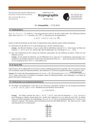
Figure 1: First Successive M<strong>in</strong>imum<br />
An example of a first successive m<strong>in</strong>imum λ1(L(a, b)) = x is the figure<br />
above.<br />
S<strong>in</strong>ce for every lattice L ⊆ R n � x �∞ ≤ � x �2 ≤ √ m � x �∞ for all<br />
x ∈ R n , it holds for the successive m<strong>in</strong>ima that<br />
λ1,∞(L) ≤ λ1,2(L) ≤ √ mλ1,∞(L)<br />
Theorem 2.9. For each lattice L ⊆ R n of rank m, � L �∞ ≤ (det L) 1<br />
m<br />
2.3 Distance Functions<br />
The term ”Distance Function” was <strong>in</strong>tegrated <strong>in</strong>to the lattice reduction theory<br />
by Lovász and Scarf.<br />
Def<strong>in</strong>ition 2.10. Let b1, b2, ...., bm ∈ R n be l<strong>in</strong>early <strong>in</strong>dependent vectors<br />
for all m ≤ n and let � · �p be an arbitrary norm on R n . The functions<br />
Fi : R n → R with<br />
Fi(x) := m<strong>in</strong>ξ1,....,ξi−1∈R � x + � i−1<br />
j=1 ξjbj �p for 1 ≤ i ≤ m + 1<br />
are called distance functions.<br />
The distance functions determ<strong>in</strong>e the distance between a vector bi and<br />
span(b1, b2, ...., bi−1) with respect to an arbitrary norm. The functions<br />
Fi(x) are actually the norm of span(b1, b2, ...., bi−1) ⊥ . With respect to<br />
the Euclidean norm they are also Euclidean norms of the subspace. The<br />
distance functions are very useful because the length of the shortest lattice<br />
vector could be restricted by them.<br />
6
Theorem 2.11. For every basis b1, b2, ...., bm of a lattice L ⊂ R n and every<br />
norm � · �p<br />
m<strong>in</strong>i=1,....,n Fi(bi) ≤ λ1,p(L)<br />
7
3 Gauss’ Algorithm<br />
The first person to develop an algorithm for lattice basis reduction was<br />
Gauss. This first algorithm generalizes the Euclidean algorithm. It was<br />
<strong>in</strong>itially described with<strong>in</strong> the general framework of b<strong>in</strong>ary <strong>in</strong>teger quadratic<br />
forms by Gauss himself and was later specified <strong>in</strong> terms of lattice basis<br />
reduction by Vallée [12]. It is the first to be considered <strong>in</strong> this paper not<br />
only because it is the first to have a polynomial-time complexity but also<br />
because it works <strong>in</strong> the 2-dimensional space and thus gives an understand<strong>in</strong>g<br />
of the higher dimensions.<br />
Primarily, the algorithm was created to work with the Euclidean norm.<br />
Later Schnorr and Kaib [4] extended the concept to an arbitrary norm. In<br />
the dissertation of Kaib [2] a detailed explanation of the generalized algorithm<br />
is given as well as an extension, that is specifically useful for the<br />
<strong>in</strong>f<strong>in</strong>ity norm.<br />
In this chapter we give a short explanation of what reduced lattice bases<br />
<strong>in</strong> the Gaussian sense mean and describe the orig<strong>in</strong>al Gauss Algorithm,<br />
which works with the Euclidean norm. This algorithm is then enhanced<br />
to work with arbitrary norms <strong>in</strong> the Generalized Gauss Algorithm. An<br />
extension for the l∞-norm and its time complexity is f<strong>in</strong>ally presented <strong>in</strong> the<br />
last sub-chapter.<br />
3.1 Gauss - reduced Bases<br />
S<strong>in</strong>ce we give a short description for both the orig<strong>in</strong>al and the generalized<br />
Gauss algorithm here, <strong>in</strong> this section � · �p, for p ∈ [1, ∞], will denote any<br />
norm.<br />
Def<strong>in</strong>ition 3.1. An ordered basis (a, b) ∈ R n is Gauss-reduced with respect<br />
to a norm � · �p when<br />
� a �p ≤ � b �p ≤ � a + b �p.<br />
When consider<strong>in</strong>g the standard <strong>in</strong>ner product for the Gram-Schmidt<br />
coefficient µ and the Euclidean norm we have:<br />
1. µ2,1 ≤ 1<br />
2 ⇔ � b �2 ≤ � a − b �2,<br />
2. µ2,1 ≥ 0 ⇔ � a − b �2 ≤ � a + b �2.<br />
Therefore the basis (a, b) is reduced if and only if<br />
1. � a �2 ≤ � b �2 and<br />
2. 0 ≤ µ2,1 ≤ 1<br />
2 .<br />
Theorem 3.2. For a reduced basis (a, b) ∈ R n , � a �p and � b �p are the<br />
two successive m<strong>in</strong>ima of the lattice L = Za + Zb.<br />
8
Def<strong>in</strong>ition 3.3. An ordered basis (a, b) ∈ R n is called well-ordered with<br />
respect to a norm � · �p when<br />
� a �p ≤ � a − b �p ≤ � b �p.<br />
The transition from an order basis to a well-ordered one could be done<br />
<strong>in</strong> few steps. We know that for the ordered basis (a, b), � a �p ≤ � b �p ≤<br />
≤ � a + b �p. If � a − b �p > � a + b �p, let b := −b. If � a �p > � a − b �p,<br />
(b − a, −a) is the well-ordered basis for this lattice.<br />
3.2 Gauss Algorithm with Euclidean <strong>Norm</strong><br />
The orig<strong>in</strong>al version of the Gaussian algorithm works with the Euclidean<br />
norm. It takes as an <strong>in</strong>put an arbitrary basis and produces as an output<br />
a basis that is reduced. In each iteration b is reduced accord<strong>in</strong>g to b :=<br />
b − ⌈µ2,1a⌋. In other words, we make b as short as possible by subtract<strong>in</strong>g<br />
a multiple of a. At the end if (a, b) is not reduced, a and b are swapped.<br />
Algorithm 1.1 Gauss <strong>Reduction</strong> Algorithm for Euclidean <strong>Norm</strong><br />
INPUT: A lattice basis (a, b) ∈ R n such that � a �2 ≤ � b �2<br />
1. WHILE |µ2,1| > 1<br />
2 DO<br />
• b := b − µa, where the <strong>in</strong>teger µ is chosen to m<strong>in</strong>imize the norm<br />
� b − µa �p.<br />
• IF � a �2 > � b �2 THEN swap a and b<br />
2. END WHILE<br />
3. DO b := b · sign(µ2,1)<br />
OUTPUT: A reduced basis (a, b) ∈ R n<br />
3.3 Generalized Gauss Algorithm<br />
The generalized Gaussian algorithm f<strong>in</strong>ds the two successive m<strong>in</strong>ima for an<br />
arbirtary norm. Given a reduced basis, we provide a m<strong>in</strong>imum size <strong>in</strong>put<br />
basis requir<strong>in</strong>g a given number of iterations. The sign of the basis vector is<br />
chosen <strong>in</strong> such a way that the algorithm iterates on a well-ordered basis. As<br />
a result all <strong>in</strong>tegral reduction coefficients µ are positive.<br />
Algorithm 1.2 Generalized Gauss Algorithm<br />
INPUT: A well-ordered lattice basis (a, b) ∈ R n<br />
1. WHILE � b �p > � a − b �pDO<br />
• b := b − µa, where the <strong>in</strong>teger µ is chosen to m<strong>in</strong>imize the norm<br />
� b − µa �p.<br />
• IF� a + b �p > � a − b �p THEN b := −b.<br />
9
• Swap a and b.<br />
2. END WHILE<br />
OUTPUT: A reduced basis (a, b) ∈ R n<br />
The exchange <strong>in</strong> Step 3 produces either a well-ordered or a reduced basis.<br />
The algorithm traverses a sequence of well-ordered bases until a reduced one<br />
is found. In order to have a well def<strong>in</strong>ed algorithm <strong>in</strong> Step 1 the smallest<br />
possible µ, that m<strong>in</strong>imizes the norm � b − µa �p for p ∈ [1, ∞], should<br />
be chosen. In general this algorithm term<strong>in</strong>ates after f<strong>in</strong>itely many steps<br />
because the norm of the basis vector decreases with every iteration, except<br />
the last one.<br />
3.4 Inf<strong>in</strong>ity <strong>Norm</strong> Algorithm<br />
As Kaib expla<strong>in</strong>s and proves <strong>in</strong> his dissertation [2] there is a fast way to<br />
calculate the coefficient µ for l∞-norm. This section describes the method<br />
proposed by him.<br />
Let us consider the function f(µ) = � b−µa �∞. It is a piecewise l<strong>in</strong>ear<br />
and convex function with at most n corners. Its m<strong>in</strong>imum, accord<strong>in</strong>g to the<br />
optimization theory, could be found on one of these corners. The reduction<br />
coefficient µ is therefore one of the two neighbor<strong>in</strong>g whole numbers of the<br />
corner that m<strong>in</strong>imizes the function f. In order to f<strong>in</strong>d that m<strong>in</strong>imum, the<br />
elements of the function f(µ) = max fi(µ)|1 ≤ i ≤ n should be taken.<br />
Let us consider the graph of the function f(x) = maxi≤n |bi − xai|, which<br />
is the maximal polygon. The ascend<strong>in</strong>g slope of the function is f + i<br />
|ai| (x − bi<br />
ai ) and the descend<strong>in</strong>g - f − i (x) := |ai| ( bi<br />
ai<br />
(x) :=<br />
− x), where all elements<br />
with ai = 0 are already elim<strong>in</strong>ated. All elements are sorted accord<strong>in</strong>g to<br />
their absolute value, |a1| ≥ |a2| ≥ .... ≥ |an| > 0 without loss of<br />
generality. Let f (k) (x) := maxi≤k |(bi − xai)| be the maximal polygon that<br />
has the k steepest elements. For each k = 1, 2, ...., n we compute the value<br />
of f (k) as an ordered subset of l<strong>in</strong>es, which build the maximal polygon. The<br />
faces of the polygon are determ<strong>in</strong>ed from these l<strong>in</strong>es and from them x (k) ,<br />
which m<strong>in</strong>imizes f (k) , is calculated.<br />
From the elements fk+1 = max (f + −<br />
k+1 , fk+1 ) only the ones with the<br />
biggest f ±<br />
k+1 (x(k) ) values are to be considered. If fk+1(x (k) ) ≤<br />
≤ f (k) (x (k) ), set f (k) = f (k+1) . In case there are more elements with the<br />
same slope, only the ascend<strong>in</strong>g one with the smallest bm<strong>in</strong><br />
am<strong>in</strong><br />
one with the biggest bmax<br />
amax<br />
are considered.<br />
and the descend<strong>in</strong>g<br />
We divide the l<strong>in</strong>e segments of f (k) <strong>in</strong> two groups - R and L, where R<br />
conta<strong>in</strong>s the ascend<strong>in</strong>g and L - the descend<strong>in</strong>g segments. The absolute value<br />
of the slope is m<strong>in</strong>imal for both groups. The value x = x (k) denotes the<br />
m<strong>in</strong>imal po<strong>in</strong>t of f (k) , that is the cross<strong>in</strong>g po<strong>in</strong>t of the topmost l<strong>in</strong>e from<br />
both groups. The biggest element from the groups is denoted by (gL, xL)<br />
10
and (gR, xR) respectively. The cross<strong>in</strong>g po<strong>in</strong>t of the two l<strong>in</strong>es is then g1 ∩<br />
g2 = b1−b2<br />
a1−a2 .<br />
We <strong>in</strong>itialize R with (g + , +∞), L with (g − , −∞) and x := g + ∩ g − . We<br />
iterate over all of the l<strong>in</strong>e, start<strong>in</strong>g with the one with the steepest slope.<br />
S<strong>in</strong>ce the two cases, with ascend<strong>in</strong>g and descend<strong>in</strong>g l<strong>in</strong>es, respectively, are<br />
symmetric, here only an algorithm only for the ascend<strong>in</strong>g case is given.<br />
Algorithm 1.3 Inf<strong>in</strong>ity <strong>Norm</strong><br />
INPUT: A well-ordered basis (a, b) ∈ R n , 0 ≤ x ≤ 1<br />
2<br />
1. ¯x := g ∩ gL<br />
2. If ¯x ≥ x, go to the next step<br />
3. As long as ¯x ≤ xL do [P OP (L, ¯x := g ∩ gL] (deletion of an element)<br />
4. x := ¯x<br />
5. ˆx := g ∩ gR<br />
6. As long as ˆx ≥ xR do [P OP (R, ˆx := g ∩ gR]<br />
7. PUSH (R, (g, ˆx)) (<strong>in</strong>sertion of an element)<br />
OUTPUT: x that m<strong>in</strong>imizes f(x) =� b − xa �∞<br />
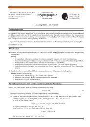
Consider the follow<strong>in</strong>g figure:<br />
This figure shows part of the graph of the function f(µ) = � b − µa �∞.<br />
The cont<strong>in</strong>ous l<strong>in</strong>es on the graph are the ones that form the polygon of the<br />
function f(x). The punctuated l<strong>in</strong>es are to be deleted by the POP function.<br />
11
3.5 Time Bounds<br />
The time bound of the generalized Gauss algorithm has been proven by<br />
Schnorr and Kaib [4]. They use the normal arithmetic operations (addition,<br />
multiplication, division, subtraction, comparison and next <strong>in</strong>teger computation)<br />
as unit costs and count arithmetical steps and oracle calls. It requires<br />
a norm oracle that produces � a �p for a given a ∈ R n , where p ∈ [1, ∞].<br />
Theorem 3.4. Given an oracle for an arbitrary norm � · �p, for p ∈ [1, ∞],<br />
there is an algorithm which � · �p-reduces a given basis (a, b) ∈ Rn us<strong>in</strong>g<br />
O(n log(n + λ2<br />
�a�p,�b�p<br />
) + log B) many steps, where B = max .<br />
λ1 λ2<br />
For efficiency, the basis is first reduced <strong>in</strong> a norm correspond<strong>in</strong>g to a<br />
suitable <strong>in</strong>ner product, that is the Euclidean norm. The result<strong>in</strong>g basis<br />
is subsequently reduced <strong>in</strong> the norm that we are <strong>in</strong>terested <strong>in</strong>. The <strong>in</strong>ner<br />
product is chosen so that {x ∈ Rn | � x �∞ ≤ 1} is spherical. The steps<br />
for produc<strong>in</strong>g the <strong>in</strong>ner product are not counted s<strong>in</strong>ce we assume they are<br />
given. The <strong>in</strong>itial <strong>in</strong>ner product reduction costs O(1) arithmetical steps per<br />
iteration.<br />
That gives a total of O(n + log B) arithmetical steps for the <strong>in</strong>ner product<br />
reduction. In each iteration the Gram-Schmidt matrix is transformed<br />
and the transformation matrix H and the coefficient µ are produced. Each<br />
iteration requires 6 multiplications, 6 subtractions, 1 division and 1 next<br />
<strong>in</strong>teger computation.<br />
The f<strong>in</strong>al � · �p-reduction is done <strong>in</strong> O(n + log(n + λ2 )) many steps. As<br />
λ1<br />
shown <strong>in</strong> the paper of Schnorr and Kaib this f<strong>in</strong>al reduction requires at most<br />
log √<br />
1+ 2 (2 √ √<br />
�x�p <br />
2 maxx,y∈Rn √ + 1) + o(1) = O(log n) many iterations.<br />
�y�p <br />
Every iteration besides the f<strong>in</strong>al one requires O(1) norm computation and<br />
O(n) arithmetical steps.<br />
The whole algorithm, which computes a reduced basis (a, b) for an arbitrary<br />
norm, works <strong>in</strong> O(n log(n + λ2 ) + log B) many steps, where B =<br />
λ1<br />
max �a�p,�b�p<br />
. λ2<br />
In the case of l∞-norm the follow<strong>in</strong>g theorem holds:<br />
Theorem 3.5. For l∞-norm there is an algorithm that reduces any given<br />
well-ordered basis (a, b) <strong>in</strong> O(n log n + log B) many iterations, where B =<br />
and λ2 is the second successive m<strong>in</strong>ima of the lattice.<br />
�b�∞<br />
λ2<br />
As presented <strong>in</strong> this section, the <strong>in</strong>ner product reduction for l∞-norm<br />
works also <strong>in</strong> O(n + log B) arithmetical steps.<br />
The algorithm, shown <strong>in</strong> the previous section, needs O(n log n) arithmetical<br />
operation for sort<strong>in</strong>g the elements. The cycle for sort<strong>in</strong>g the l<strong>in</strong>es<br />
costs at most O(n) arithmetical operations. There is only one PUSH step<br />
for each element and at most n − 1 POP steps.<br />
12
Hence the l∞-norm reduction of a lattice basis (a, b) ∈ Rn takes at most<br />
O(n log n + log B) arithmetical steps, where B = �b�∞<br />
and λ2 is the second<br />
λ2<br />
successive m<strong>in</strong>ima of the lattice.<br />
13
4 LLL<br />
The subject of lattice basis reduction theory was revived <strong>in</strong> 1981 with<br />
H.W.Lenstra’s work on <strong>in</strong>teger programm<strong>in</strong>g, which is based on a novel<br />
lattice reduction technique and works <strong>in</strong> polynomial time only for fixed dimensions.<br />
Lovász later developed a version of the algorithm which computes<br />
a reduced basis of a lattice <strong>in</strong> polynomial time for any dimension. The LLL<br />
algorithm, named after its creators, reached its f<strong>in</strong>al version <strong>in</strong> the paper of<br />
A.K. Lenstra, H.W. Lenstra and L. Lovász [7], where it is applied to factor<br />
rational polynomials with respect to the Euclidean norm. It computes<br />
a reduced basis after polynomial many steps. Further enhancements were<br />
<strong>in</strong>troduced later by Schnorr.<br />
In 1992 Lovász and Scarf [8] proposed a generalized lattice reduction algorithm,<br />
which was later named after them - LS algorithm. They extend the<br />
mean<strong>in</strong>g of an LLL-reduced basis to any norm. It works <strong>in</strong> polynomial many<br />
arithmetical operations and calculations of distance functions.<br />
We beg<strong>in</strong> this chapter with a short description of the mathematical mean<strong>in</strong>g<br />
of LLL-reduced bases. The orig<strong>in</strong>al LLL algorithm is then presented.<br />
This type of reduction is cont<strong>in</strong>ued with the LS algorithm that works with<br />
an arbitrary norm. F<strong>in</strong>ally, a specific enumeration for the <strong>in</strong>f<strong>in</strong>ity norm is<br />
<strong>in</strong>troduced.<br />
4.1 LLL-reduced <strong>Basis</strong><br />
Here we expla<strong>in</strong> the mean<strong>in</strong>g of an LLL-reduced basis and show the qualities<br />
of such a basis. Let ( ˆ b1, ˆ b2, ..., ˆ bm) be the ordered orthogonal system for<br />
the basis (b1, b2, ..., bm) ∈ R n and µi,j the Gram-Schmidt coefficient.<br />
Def<strong>in</strong>ition 4.1. An ordered lattice basis (b1, b2, ...., bm) ∈ Rn is called<br />
< δ ≤ 1, when:<br />
LLL-reduced for a parameter δ, such that 1<br />
4<br />
1. |µi,j| ≤ 1<br />
2<br />
for 1 ≤ j < i ≤ m<br />
2. δ · � ˆ bk−1 �2 2 ≤ � ˆ bk �2 2 + µ2 k,k−1 · � ˆ bk−1 �2 2 , for k = 2, 3, ...., m<br />
The quality of the reduced basis depends on the parameter δ : the bigger<br />
the value, the stronger the reduction of the basis. In the orig<strong>in</strong>al paper of<br />
Lenstra, Lenstra and Lovász the LLL algorithm is def<strong>in</strong>ed only for δ = 3<br />
4 .<br />
With the help of the orthogonal projection<br />
πk : R n → span(b1, b2, ...., bk−1) ⊥ .<br />
The second part of the def<strong>in</strong>ition could be written <strong>in</strong> the follow<strong>in</strong>g way:<br />
δ · � πk−1(bk−1) �2 2 ≤ � πk−1(bk) �2 2 , for k = 2, 3, ...., m.<br />
14
In the case where the basis consists of only two vectors, for δ = 1 we<br />
get a Gauss reduced basis.<br />
If (b1, b2, ...., bm) is LLL-reduced with some δ then (πk(bk), πk(bk+1),<br />
..., πk(bj)) is also LLL-reduced with δ and 1 ≤ k < j ≤ n.<br />
Theorem 4.2. Let (b1, b2, ...., bm) be LLL-reduced for the parameter δ. For<br />
we have<br />
α = 1<br />
δ− 1<br />
4<br />
� ˆ bi � 2 2 ≤ αj−i · � ˆ bj � 2 2<br />
for 1 ≤ i ≤ j ≤ m.<br />
For the special case of δ = 3<br />
4 and α = 2 we have � b1 � 2 2 ≤ 2j−1 · � ˆ bj � 2 2<br />
so that the square of the length for big values of j is not arbitrary small.<br />
Theorem 4.3. Let (b1, b2, ...., bm) be a basis of the lattice L ⊂ R n . Then<br />
for i = 1, 2, ...., m we have<br />
λj ≥ m<strong>in</strong>i=j,j+1,...,m � ˆ bi �2.<br />
This theorem shows that the lengths � ˆ bj �2 are a rough approximation<br />
of the successive m<strong>in</strong>ima λj.<br />
Theorem 4.4. Let (b1, b2, ...., bm) be the basis of the lattice L ⊆ Rn with<br />
a parameter δ. It holds for α = 1<br />
δ− 1<br />
4<br />
that :<br />
1. α1−j ≤ �ˆ bj�2 2<br />
λ2 , for j = 1, 2, ...., m,<br />
j<br />
2. �bj� 2 2<br />
λ 2 j<br />
≤ α n−1 , for j = 1, 2, ...., m,<br />
3. � bk �2 2 ≤ αj−1 · � ˆ bj �2 2 , for k ≤ j.<br />
Def<strong>in</strong>ition 4.5. Let � · �p for p ∈ [1, ∞] be any norm <strong>in</strong> R n and 0 < ∆ ≤ 1.<br />
A basis b1, b2 , ..., bm of a lattice L ⊂ R n is called Lovász-Scarf reduced<br />
with ∆ or LS-reduced with ∆ if<br />
1. Fj(bi) ≤ Fj(bi ± bj), for all j < i,<br />
2. ∆Fi(bi) ≤ Fi(bi+1), for 1 ≤ j < m.<br />
In the case of the Euclidean norm, the terms δ LLL-reduced lattice basis<br />
and ∆ = √ δ LS-reduced lattice basis are equivalent. The bigger the value<br />
of ∆, the stronger the basis reduction.<br />
Theorem 4.6. For each LS-reduced basis (b1, b2, ...., bm) of a lattice L ⊂<br />
Rn with ∆ ∈ ( 1<br />
2 , 1] the follow<strong>in</strong>g holds:<br />
(∆ − 1<br />
2 )i−1 ≤ Fi(bi)<br />
λi,�·�p (L) ≤ (∆ − 1<br />
2 )i−m , for i = 1, ....., m.<br />
15
4.2 LLL Algorithm<br />
Algorithm 2.1 LLL Algorithm<br />
Input : A basis (b1, b2, ...., bm) ∈ R n δ with 0 ≤ δ ≤ 1<br />
1. k := 2 (k is the stage)<br />
[Compute the Gram-Schmidt coefficient µi,j for 1 ≤ j < i < k<br />
and ci = � ˆ bi �2 2 for i = 1, ...., k − 1]<br />
2. WHILE k ≤ n<br />
• IF k = 2 THEN c1 := � b1 � 2 2<br />
• FOR j = 1, ...., k − 1<br />
µk,j := (〈 bk,bk 〉 − � j−1<br />
i=1 µj,iµk,ici)<br />
cj<br />
• ck := 〈 bk, bk 〉 − � k−1<br />
j=1 µk,jcj<br />
3. Reduce the size of bk<br />
• FOR j = k − 1, ...., 1<br />
– µ := ⌈µk,j⌋<br />
– FOR i = 1, ...., j − 1 : µk,j := µk,i − µµj,i<br />
– µk,j := µk,j − µ<br />
– bk := bk − µbj<br />
4. • IF δck−1 > ck + µ 2 k,k−1 ck−1<br />
• THEN swap bk and bk−1 , k := max(k − 1, 2)<br />
• ELSE k := k + 1<br />
5. END while<br />
OUTPUT : an LLL-reduced basis (b1, b2, ...., bm) ∈ Rn with δ<br />
In step 1, when enter<strong>in</strong>g degree k, the basis (b1, b2, ...., bk−1) is already<br />
LLL-reduced with a parameter δ and the Gram-Schmidt coefficients µi,j, for<br />
1 ≤ j < i < k, as well as the values ci = � ˆ bi �2 2 , for i = 1, ...., k − 1,<br />
are already available.<br />
Step 3 is actually an algorithm that reduces the size of the basis. For<br />
additional <strong>in</strong>formation on this algorithm see the lecture slides of Schnorr.<br />
For the swap of bk and bk−1 the values � ˆ bk �2 2 , � ˆ bk−1 �2 2 and µi,j, µj,i,<br />
for j = k − 1, k and i = 1, 2, ...., m, have to be calculated aga<strong>in</strong>. It is<br />
important to keep the basis <strong>in</strong> exact arithmetics because otherwise a change<br />
<strong>in</strong> the lattice would be made that cannot be fixed.<br />
Let B denote max(� b1 �2 2 , � b2 �2 2 , ...., � bm �2 2 ) for the <strong>in</strong>put basis.<br />
Throughout the algorithm the bit length of the numerators and denom<strong>in</strong>ators<br />
of the rational numbers � ˆ bi �2 2 , µi,j is bounded by O(m log B). The<br />
16
it length of the coefficients of the bi ∈ Z n is also bounded by O(m log B)<br />
throughout the algorithm.<br />
The algorithm preforms at most O(m 3 n log B) arithmetic operations on <strong>in</strong>tegers<br />
that are O(m log B) bits long.<br />
4.3 LS Algorithm<br />
Lovász and Scarf [8] <strong>in</strong>troduced <strong>in</strong> 1992 an algorithm that gives a reduced<br />
basis for an arbitrary norm <strong>in</strong> polynomial many steps with respect to the<br />
size of the <strong>in</strong>put.<br />
Algorithm 2.2 LS Algorithm<br />
INPUT : A basis (b1, b2, ...., bm) ∈ R n , ∆ with 0 ≤ ∆ ≤ 1<br />
1. k := 2<br />
2. WHILE k ≤ n<br />
• Reduce the length of bk<br />
3. END while<br />
– FOR j = k − 1, ...., 1<br />
∗ Compute a whole number µj which m<strong>in</strong>imizes<br />
Fj(bk − µbj)<br />
∗ bk := bk − µbj<br />
– IF Fk−1(bk) < ∆Fk−1(bk−1)<br />
– THEN swap bk and bk−1 , k := max(k − 1, 2)<br />
– ELSE k := k + 1<br />
OUTPUT : an LS-reduced basis b1, b2, ...., bm with a parameter ∆<br />
In each step of the algorithm we search for the first <strong>in</strong>dex k − 1 for which<br />
one of the conditions<br />
1. Fk−1(bk + µbj) ≥ Fk−1(bk) for <strong>in</strong>tegral µ,<br />
2. Fk−1(bk) ≥ ∆Fk−1(bk−1)<br />
is not satisfied, where F is a distance function. If the first condition is not<br />
satisfied we replace bk by bk + µjbj, with µ be<strong>in</strong>g the <strong>in</strong>teger that m<strong>in</strong>imizes<br />
Fk−1(bk +µbj). If after the replacement the second condition holds we move<br />
to level k. If the second condition is not satisfied, we <strong>in</strong>terchange bk and<br />
bk−1 and move to the correspond<strong>in</strong>g level.<br />
Notice that the maximum value of the components of the vector F1(b1),<br />
..., Fk−1(b k−1 ), Fk(bk), ..., Fm(bm), consist<strong>in</strong>g of distance functions, does<br />
not <strong>in</strong>crease at any step of the basis reduction algorithm. If we replace bk<br />
by bk + µjbj, none of the terms actually change. If bk and bk−1 are<br />
<strong>in</strong>terchanged, Fk−1(bk−1) simply becomes Fk−1(bk) ≤ ∆Fk−1(bk).<br />
17
4.4 Comput<strong>in</strong>g the Distance Functions <strong>in</strong> Inf<strong>in</strong>ity <strong>Norm</strong><br />
The problem of comput<strong>in</strong>g the distance functions for the l∞-norm is actually<br />
an optimization problem:<br />
Given is a basis b1, b2, ...., bm and x ∈ R n .<br />
Compute Fi(x) = m<strong>in</strong>zi∈R � x + � i−1<br />
j=1 zjbj �∞ such that<br />
s.t.<br />
zi ≥ 0 (1)<br />
zi := � x +<br />
−zi ≤ xk +<br />
�i−1<br />
j=1<br />
zjbj �∞<br />
(2)<br />
�i−1<br />
zjbj,k ≤ zi, for all k = 1, ...., m (3)<br />
j=1<br />
We get the follow<strong>in</strong>g optimization problem:<br />
M<strong>in</strong>imize Q(x) = zi<br />
zi ≥ 0 (4)<br />
zi ≤ � x �∞ (5)<br />
�i−1<br />
zjbj,k − zi ≤ −xk (6)<br />
j=1<br />
�i−1<br />
− zjbj,k − zi ≤ xk, for all k = 1, ...., m (7)<br />
j=1<br />
Such an optimization problem is solved <strong>in</strong> polynomial time for all rational<br />
<strong>in</strong>put values with the help of the Ellipsoid Method or the Karmarkars<br />
Algorithm. In practice the Simplex Algorithm is even more efficient.<br />
The best and quickest way to solve such a problem would be to use the<br />
ILOG CPLEX Software, which is a large-scale programm<strong>in</strong>g software that<br />
is capable of solv<strong>in</strong>g huge, real-world optimization problem. The problem is<br />
simply written <strong>in</strong> the respective CPLEX language and the software f<strong>in</strong>ds a<br />
solution if there is such.<br />
Another option is to model the problem <strong>in</strong> a language that translates the<br />
mathematical model <strong>in</strong>to a l<strong>in</strong>ear or mixed-<strong>in</strong>teger mathematical program,<br />
like for example Zimpl [5], and solve the result<strong>in</strong>g problem us<strong>in</strong>g JAVA. This<br />
approach is not as quick and affective as the first one but is the only way to<br />
solve such an optimization problem without expensive software.<br />
18
4.5 Time Bounds<br />
The LS basis algorithm is known to converge <strong>in</strong> polynomial time, <strong>in</strong>clud<strong>in</strong>g<br />
the number of variables n, for F (x) = |x| and a general lattice given by an<br />
<strong>in</strong>teger basis. This argument is based on two observations:<br />
1. An <strong>in</strong>terchange between bk−1 and bk preserves the value of the distance<br />
function for all <strong>in</strong>dices other than k and k − 1.<br />
2. For F (x) = |x|, the product Fk−1(bk−1)Fk(bk) is constant when the<br />
vectors bk−1 and bk are exchanged. This permits us to deduce that<br />
� (Fk−1(bk−1)) m−1 decreases by a factor ∆ at each <strong>in</strong>terchange.<br />
� (Fk−1(bk−1)) m−1 ≥ 1 is therefore true for any basis, from which<br />
the polynomial convergence follows.<br />
The product Fk−1(bk−1)Fk(bk) is not constant <strong>in</strong> the general case, and<br />
therefore the algorithm does not execute <strong>in</strong> polynomial time with respect to<br />
the number of variables m. However it could be shown that the algorithm<br />
works <strong>in</strong> polynomial time for a fixed m. There are two arguments to support<br />
this conclusion both of which are go<strong>in</strong>g to be expla<strong>in</strong>ed here briefly. They<br />
are both fully covered <strong>in</strong> the paper of Lovász and Scarf [7].<br />
The idea beh<strong>in</strong>d both of them is to obta<strong>in</strong> a lower bound for the values<br />
of Fi(bi). For this purpose, let C ⊂ B(R) be a ball of radius R.<br />
The distance function F (x) ≥ |x|<br />
R . Let b1, b2, ...., bm be any basis that<br />
satisfies Fi(bi) ≤ U where U is equal to max Fi(ai). We have that<br />
ci = bi + � i−1<br />
j=1 µi,jbj is a proper basis associated with bi, satisfy<strong>in</strong>g<br />
Fi(ci) = Fi(bi) and F1(ci) ≤ Fi(bi) + 1 �i−1 2 1 Fi(bj) ≤ mU. Therefore<br />
we get that |ci| ≤ mUR.<br />
The distance function is limited from below by the follow<strong>in</strong>g <strong>in</strong>equality:<br />
Fi(bi) ≥ m<strong>in</strong> |(bi + α1c1 + .... + αi−1ci−1)|<br />
R<br />
.<br />
This actually represents the distance between the vector bi and the space<br />
< c1, ...., ci−1 >. When this distance is represented by the Gram matrix<br />
G(x1, ...., xi) = det[(xj, xk)] i j,k=1 , for the <strong>in</strong>tegral bj and c1, ...., ci−1 we<br />
get that G(c1, ...., ci−1, bj) ≥ 1. From there it can be concluded that<br />
Fi(bi) ≥ 1/[R(mRU) i−1 ] ≥ 1/[R(mRU) n−1 ]. Set here Fi(bi) to be equal<br />
to V .<br />
As we already mentioned, each component of F1(b1), ..., Fi(bi),<br />
Fi+1(bi+1), ..., Fm(bm) is bounded above by max Fi(ai) = U throughout<br />
the algorithm. Scarf and Lovász also noticed that the first term <strong>in</strong> the<br />
sequence to change at any iteration decreases by a factor of (1 − ɛ).<br />
The first argument for the polynomial convergence of the generalized<br />
algorithm is therefore to observe that the maximum number of <strong>in</strong>terchanges<br />
is<br />
[log(U/V )/ log(1/(1 − ɛ))] m<br />
19
Us<strong>in</strong>g the <strong>in</strong>troduced lower bound V , it can be seen that the <strong>in</strong>terchanges<br />
of the basis reduction algorithm is bounded above by :<br />
[m log(mUR)/ log(1/(1 − ɛ))] m<br />
The second argument for polynomiality, which achieves a different bound,<br />
depends on the observation that for a general distance function the product<br />
Fi(bi) Fi+1(bi+1) <strong>in</strong>creases by a factor ≤ 2 <strong>in</strong> any step of the algorithm<br />
for an <strong>in</strong>terchange of bi and bi+1. Here Fi(bi) = 1. Let y = bi and x =<br />
bi+1<br />
Fi(bi+1) . Fi+1(x) = 1 and F ∗<br />
dx i+1 (bi) = 1 with F ∗<br />
dx i+1 the distance function<br />
associated with a projection of the orig<strong>in</strong>al basis <strong>in</strong>to < bi, bi+2, ...., bm >.<br />
Therefore<br />
Fi(bi+1)F ∗<br />
i+1 (bi)/Fi(bi)Fi+1(bi+1) =<br />
= [ Fi(bi+1)<br />
dy<br />
]/[ Fi(bi+1)<br />
dx<br />
] = dx/dy ≤ 2<br />
Let D(b1, ...., bm) = � (Fi(bi)) γm−1,<br />
with γ = 2 +<br />
1<br />
1<br />
log( (1 − ɛ)<br />
). It is<br />
easy to see that D(b1, ...., bm) decreases by a factor of at least 1 − ɛ at each<br />
<strong>in</strong>terchange required by the basis reduction algorithm. S<strong>in</strong>ce V ≤ Fi(bi) ≤ U<br />
at each step of the algorithm , the number of <strong>in</strong>terchanges is bounded above<br />
by:<br />
[(γ m − 1)/(γ − 1)] log(U/V ) log(1/(1 − ɛ))<br />
≤ (γ n − 1)/(γ − 1)]m log(mUV ) log(1/(1 − ɛ))<br />
.<br />
This second estimate is much better than the first one <strong>in</strong> terms of its<br />
dependence to U and R. And s<strong>in</strong>ce the number of possible values of the vector<br />
F1(b1), ...., Fi(bi), Fi+1(bi+1), ...., Fm(bm) is f<strong>in</strong>ite, the basis reduction<br />
algorithm executes <strong>in</strong> f<strong>in</strong>ite time even when ɛ = 0.<br />
20
5 Block-Kork<strong>in</strong>e-Zolotarev Algorithm<br />
The algorithms presented <strong>in</strong> the previous section - LLL and LS, produce<br />
a reduced basis <strong>in</strong> polynomial time with respect to the <strong>in</strong>put data but the<br />
result is only an approximation of the actual shortest lattice vector with<br />
an exception of an exponential factor. In order to improve the practical<br />
usage of these algorithms, Schnorr developed a hierarchy of reduction terms<br />
with respect to the Euclidean norm, the so called block reduction. The<br />
new algorithm, that Schnorr created, covers the general case of lattice basis<br />
us<strong>in</strong>g the LLL-reduced and the HKZ-reduced (Hermite-Kork<strong>in</strong>e-Zolotarev,<br />
for more <strong>in</strong>formation see the script of Schnorr) bases as extreme cases.<br />
In this chapter we present the practical BKZ algorithm and the subrout<strong>in</strong>e<br />
ENUM which work with respect to the Euclidean norm. This block<br />
reduction theory is then expanded to an arbitrary norm and an algorithm<br />
deal<strong>in</strong>g specifically with the <strong>in</strong>f<strong>in</strong>ity norm is f<strong>in</strong>ally expla<strong>in</strong>ed.<br />
5.1 BKZ-reduced lattice basis<br />
Let L = L(b1, b2, ...., bm) ∈ R n be a lattice with an ordered basis<br />
b1, b2, ...., bm. Furthermore, πi : R m ⇒ span(b1, b2, ...., bm) holds true.<br />
Let Li denote the lattice πi(L), which is a lattice of rank m − i + 1.<br />
Def<strong>in</strong>ition 5.1. An ordered basis b1, b2, ...., bm ∈ Rn is called size-reduced<br />
if |µi,j| ≤ 1<br />
2 for 1 ≤ j < i ≤ m An <strong>in</strong>dividual basis vector bi is<br />
for 1 ≤ j < i.<br />
size-reduced if |µi,j| ≤ 1<br />
2<br />
Def<strong>in</strong>ition 5.2. An ordered basis b1, b2, ...., bm of a lattice L ⊂ R n is called<br />
a Kork<strong>in</strong>e-Zolotarev basis if:<br />
1. it is size-reduced,<br />
2. � ˆ bi �2 = λ1(Li), for i = 1, ...., m.<br />
This def<strong>in</strong>ition is equivalent to the orig<strong>in</strong>al def<strong>in</strong>ition given <strong>in</strong> Kork<strong>in</strong>e<br />
and Zolotarev’s book from 1873.<br />
Theorem 5.3. Let β be an <strong>in</strong>teger such that 2 ≤ β < n. A lattice basis<br />
b1, b2, ...., bm is β-reduced if:<br />
1. it is size-reduced,<br />
2. � ˆ bi �2 ≤ λi(Li(b1, b2, ...., b m<strong>in</strong>(i+β−1,m))), for i = 1, ...., m − 1.<br />
Let αβ denote the maximum of �b1�2<br />
�bβ�2<br />
over all Kork<strong>in</strong>e-Zolotarev reduced<br />
bases. For ln β - the natural logarithm of β, α2 = 3<br />
1<br />
4 , α3 = 3<br />
2 and<br />
αβ ≤ β1+ln β (β−1)<br />
. The constra<strong>in</strong>t αβ<br />
converges to 1 with the <strong>in</strong>crease of β.<br />
The follow<strong>in</strong>g theorem shows the strength of a β-reduced basis <strong>in</strong> comparison<br />
to an LLL-reduced one.<br />
21
Theorem 5.4. Every β-reduced basis b1, b2, ...., bm of a lattice L ⊂ R n<br />
satisfies � b1 � 2 2<br />
≤ α<br />
(n−1)<br />
β−1<br />
β<br />
λ1(L) 2 provided that β − 1 divides n − 1.<br />
Def<strong>in</strong>ition 5.5. A basis b1, b2, ...., bm is called β-reduced with a parameter<br />
< δ ≤ 1 if:<br />
δ for 1<br />
4<br />
1. it is size-reduced,<br />
2. δ � ˆ bi � 2 2 ≤ λ1(Li(b1, b2, ...., b max(i+β−1,m))) 2 , for i = 1, ...., m.<br />
Notice that for β = 2 and 1<br />
3<br />
actually an LLL-reduced basis.<br />
≤ δ ≤ 1, a (β, δ)-reduced basis is<br />
Def<strong>in</strong>ition 5.6. A lattice basis b1, b2, ...., bm is called β-block reduced with<br />
a parameter δ, for 1<br />
2 ≤ δ ≤ 1 and i = 1, ...., m, if for the distance function<br />
F the follow<strong>in</strong>g two <strong>in</strong>equations hold true:<br />
1. δFi(bi) ≤ m<strong>in</strong> Fi(b), where b ∈ Zbi + .... + Zb m<strong>in</strong>(i+β−1,m) − 0,<br />
2. Fj(bi) ≤ Fj(bi ± bj), for all j < i.<br />
5.2 BKZ Algorithm with Euclidean <strong>Norm</strong><br />
The follow<strong>in</strong>g algorithm performs a β-reduction with respect to a parameter<br />
δ. Its backbone is the subrout<strong>in</strong>e ENUM(j, k), which is also presented <strong>in</strong><br />
this section.<br />
Algorithm 3.1 BKZ Algorithm with Euclidean <strong>Norm</strong><br />
INPUT: A lattice basis b1, b2, ...., bm ∈ Z n with parameters δ, with<br />
0 ≤ δ ≤ 1, and β, with 2 < β < m<br />
1. Size-reduce b1, b2, ...., bβ; j := m − 1; z := 0<br />
2. WHILE z < m − 1<br />
• j := j + 1, IF j = m THEN j := 1<br />
• k := m<strong>in</strong>(j + β − 1, m)<br />
• ENUM(j, k) (ENUM f<strong>in</strong>ds the whole numbers (uj, ...., uk) from<br />
the representation of the vectors bnew j<br />
πj(bnew j ) �2 2 = λ2 1,�·�2 (L(πj(bj), ...., πj(bk))))<br />
• h := m<strong>in</strong>(k + 1, m)<br />
• IF ¯cj < δcj<br />
• THEN<br />
– extend b1, b2, ...., bj−1, bnew to a basis<br />
b1, b2, ...., bj−1, b new<br />
j<br />
– size-reduce b1, b2, ...., bj−1, b new<br />
j<br />
j<br />
= � k<br />
i=j uibi with ¯cj := �<br />
, ...., b new<br />
k , bk+1, ...., bm of a lattice L<br />
22<br />
, ...., b new<br />
h
– z := 0<br />
• ELSE<br />
3. END WHILE<br />
– size-reduce b1, b2, ...., bm<br />
– z := z + 1<br />
OUTPUT: BKZ-reduced basis b1, b2, ...., bm<br />
Throughout the algorithm the <strong>in</strong>teger j is cyclically shifted through the<br />
<strong>in</strong>tegers 1, 2, ...., m − 1. The variable z counts the number of positions j<br />
which satisfy the <strong>in</strong>equality<br />
δ � ˆ bj � 2 2 ≤ λ2 1,�·�2 (L(πj(bj), ...., πj(bk))).<br />
If this <strong>in</strong>equality does not hold for some j, then bnew j would be <strong>in</strong>serted<br />
<strong>in</strong>to the basis, a size-reduction would be done and z would be reset to 0.<br />
The term j = m is skipped s<strong>in</strong>ce the <strong>in</strong>equality always holds for it. As<br />
def<strong>in</strong>ed earlier, a basis b1, b2, ...., bm is β-reduced with a parameter δ if it<br />
is size-reduced and z = m − 1. Therefore, the algorithm always produces<br />
a β-block reduced basis with a parameter δ up to a certa<strong>in</strong> error.<br />
The size reduction <strong>in</strong> step one could be alternatively replaced either by<br />
an LLL-reduction or an L3FP-reduction (LLL Float<strong>in</strong>g Po<strong>in</strong>t-reduction).<br />
When add<strong>in</strong>g the vectors b1, b2, ...., bj−1, bnew j = �k i=j uibi we differentiate<br />
between several cases for g := max i : j ≤ i ≤ k, ui �= 0:<br />
1. |ug| = 1: b1, b2, ...., bnew j , bj, ...., bg−1, bg+1, ...., bm is a basis of the<br />
lattice. This means that the vector bg could be removed from the<br />
.<br />
lattice and replaced by b new<br />
j<br />
2. |ug| > 1: In this case the basis b1, b2, ...., bm is transformed <strong>in</strong>to b1,<br />
b2, ..., bj−1, b ′<br />
j , ..., b′ g, bg+1, ...., bm such that bnew j =� g<br />
i=j u′ ib′ i with<br />
|u ′<br />
i | = 1. This is always possible when the result of the subrout<strong>in</strong>e<br />
ENUM(j, k) holds, thus when ggT (uj, ...., uk) = 1 holds. Otherwise<br />
b :=<br />
bnew j<br />
ggT (uj,....,uk) is a lattice vector for which � πj(b) �2 2 =<br />
ĉj<br />
ggT (uj,....,uk) 2<br />
and therefore ĉj>λ 2 1,�·�2 (L(πj(bj), ..., πj(bk))). The vector b ′<br />
removed from the basis and replaced by b new<br />
j<br />
.<br />
j<br />
is then<br />
As mentioned before, the core of this algorithm is actually the rout<strong>in</strong>e<br />
ENUM(j, k), which computes the vectors for which the distance function<br />
Fj is m<strong>in</strong>imal. We are look<strong>in</strong>g here for <strong>in</strong>tegers (uj, ...., uk) �= (0, ...., 0)<br />
and ¯ Fj := Fj( � k<br />
i=j uibi) = λ1,Fj (L(bj, ...., bk)). This is done with the<br />
help of a recursive enumeration of all coefficient vectors (ũt, ...., ũk) ∈ Z k−t+1 ,<br />
for t = k, ...., j and Ft( � k<br />
i=t ũibi) < Fj(bj). For the coefficient vector<br />
different from 0, for which Fj is m<strong>in</strong>imal throughout the whole enumeration,<br />
the <strong>in</strong>tegers (uj, ...., uk) are set to (ũj, ...., ũk).<br />
23
For each step t > p of the algorithm, the <strong>in</strong>tegers (ũt+1, ...., ũs) are fixed.<br />
All left <strong>in</strong>tegers ut−1, for which Ft( �k i=t ũibi) < Fj(bj), are enumerated.<br />
S<strong>in</strong>ce Ft(−x) = Ft(x) for all x ∈ Rn if ũk = .... = ũt = 0 we<br />
could limit the search to only nonnegative <strong>in</strong>tegers. Every time a coefficient<br />
is computed it is organized <strong>in</strong> a search tree with depth k − j + 2.<br />
Currently the Depth-First-Search is considered most appropriate for the<br />
enumeration. With respect to the Euclidean norm and z ∈ R, the distance<br />
function Ft can be efficiently computed with the help of the Gram-Schmidt<br />
orthogonal system. From<br />
˜ct := � πt( �k i=t ũibi) �2 2 and ct := � ˆ bt �2 2 = � πt(bt) �2 2 , for 1 ≤ t ≤ k<br />
we get<br />
F 2 t ( � k<br />
i=t ũibi) = ˜ct = ˜ct+1 + (ũt + � k<br />
i=t+1 ũiµi,t) 2 ct<br />
−yt is the m<strong>in</strong>imal real po<strong>in</strong>t for yt := � k<br />
i=t+1 ũiµi,t. We get the whole<br />
m<strong>in</strong>imum through the symmetry<br />
ct(−yt + x, ũt+1, ...., ũk) = ct(−yt − x, ũt+1, ...., ũk)<br />
at the po<strong>in</strong>t νt := ⌈−yt⌋. Depend<strong>in</strong>g on whether νt > −yt holds true or<br />
not, we get a sequence of non-decl<strong>in</strong><strong>in</strong>g values ˜ct either <strong>in</strong> order (νt, νt − 1,<br />
νt + 1, νt − 2, ...) or <strong>in</strong> order (νt, νt + 1, νt − 1, νt + 2, ....).<br />
Algorithm 3.2 ENUM with Euclidean <strong>Norm</strong><br />
INPUT: j, k, b1, ...., bm<br />
1. • s := t := j, ¯cj := cj, ũj := uj := 1<br />
• νj := yj := ∆j := 0, δj := 1<br />
• FOR i = j + 1, ...., k + 1<br />
– ˜ci := ui := ũi := νi := ∆i := 0<br />
– δi := 1<br />
2. WHILE t ≤ k<br />
• ˜ct := ˜ct+1 + (yt + ũt) 2 ct<br />
• IF ˜ct < ¯cj<br />
• THEN<br />
– IF t > j<br />
– THEN<br />
∗ t := t − 1, yt := � s<br />
i=t+1 ũiµi,t<br />
∗ ũt := νt := ⌈−yt⌋, ∆t := 0<br />
∗ IF ũt > −yt<br />
∗ THEN δt := −1<br />
∗ ELSE δt := 1<br />
24
– ELSE ¯cj := ˜cj, ui := ˜ci, for i = j, ...., k<br />
• ELSE<br />
3. END WHILE<br />
– t := t + 1<br />
– s := max(s, t)<br />
– IF t < s THEN ∆t := −∆t<br />
– IF ∆tδt ≥ 0 THEN ∆ := ∆ + δt<br />
– ũt := νt + ∆t<br />
OUTPUT: The m<strong>in</strong>imal po<strong>in</strong>t (uj, ...., uk) ∈ Z k−j+1 − 0 k−j+1 and the<br />
m<strong>in</strong>imum ¯cj(uj, ...., uk)<br />
With a proper prereduction of the lattice basis, this algorithm gives a<br />
shortest lattice vector consist<strong>in</strong>g only of <strong>in</strong>tegers. This rout<strong>in</strong>e f<strong>in</strong>ds the<br />
shortest vector with respect to the Euclidean norm up to a dimension 50<br />
by sett<strong>in</strong>g j = 1 and k := m. When it is used as a subrout<strong>in</strong>e of a<br />
(β, δ)-block reduction with δ < 1 only the vectors b new<br />
j with ¯c < δcj<br />
are of <strong>in</strong>terest. The costs could be therefore reduced from the beg<strong>in</strong>n<strong>in</strong>g by<br />
sett<strong>in</strong>g ¯cj := δcj.<br />
5.3 BKZ Algorithm with an Arbitrary <strong>Norm</strong><br />
The BKZ Algorithm with an arbitrary norm is analogous to the one with<br />
the Euclidean norm. Instead of ¯cj here the distance functions are used.<br />
Algorithm 3.3 BKZ Algorithm with an Arbitrary <strong>Norm</strong><br />
INPUT: A lattice basis b1, b2, ...., bm ∈ Z n with parameters δ with<br />
0 ≤ δ ≤ 1 and β with 2 ≤ β ≤ m<br />
1. Size-reduce b1, b2, ...., bβ; j := m − 1; z := 0<br />
2. WHILE z < m − 1<br />
• j := j + 1, IF j = m THEN j := 1<br />
• k := m<strong>in</strong>(j + β − 1, m)<br />
• ENUM(j, k) (ENUM f<strong>in</strong>ds the whole numbers (uj, ...., uk) from<br />
the representation of the vectors bnew j = �k i=j uibi with<br />
¯Fj := Fj( �k i=j uibi))<br />
• h := m<strong>in</strong>(k + 1, m)<br />
• IF ¯ Fj < δFj(bj)<br />
• THEN<br />
– extend b1, b2, ...., bj−1, bnew to a basis<br />
b1, b2, ...., bj−1, b new<br />
j<br />
– size-reduce b1, b2, ...., bj−1, b new<br />
j<br />
j<br />
, ...., b new<br />
k , bk+1, ...., bm of a lattice L<br />
25<br />
, ...., b new<br />
h
– z := 0<br />
• ELSE<br />
3. END WHILE<br />
– size-reduce b1, b2, ...., bm<br />
– z := z + 1<br />
OUTPUT: BKZ-reduced basis b1, b2, ...., bm<br />
The same logic is applied here as <strong>in</strong> the algorithm that works with respect<br />
to the Euclidean norm. j is cyclically shifted through the <strong>in</strong>tegers<br />
1, 2, ...., m − 1. The variable z counts the number of positions j which satisfy<br />
the <strong>in</strong>equality δFj(bj) < ¯ Fj. Here aga<strong>in</strong>, if the <strong>in</strong>equality does not<br />
hold, bnew is <strong>in</strong>serted <strong>in</strong>to the basis, a size-reduction is done and z is set to<br />
j<br />
0. The term j = m is skipped s<strong>in</strong>ce for it the <strong>in</strong>equality always holds. The<br />
basis (b1, b2, ...., bj−1, b new<br />
j<br />
) is extended to (b1, b2, ...., bj−1, b new<br />
j<br />
us<strong>in</strong>g the coefficients uj <strong>in</strong> the representation bnew j<br />
, ...., b new<br />
h )<br />
= � h<br />
i−j uibi. The ma-<br />
trix T ∈ GLh−j+1(Z) with [uj, ...., uh] · T = [1, 0, ...., 0] is computed at this<br />
po<strong>in</strong>t and the vectors [bnew j , ...., bnew h ] are set to [bj, ...., bh] · T −1 .<br />
The backbone of the algorithm is aga<strong>in</strong> the rout<strong>in</strong>e ENUM(j, k), which<br />
computes the m<strong>in</strong>imal po<strong>in</strong>t (uj, ...., uk) so that the m<strong>in</strong>imum of ¯ Fj can be<br />
found. Here we are look<strong>in</strong>g for a vector b ∈ L(b1, b2, ..., bm) ⊂ Rn with<br />
� b �p = λ1,�·�p (L). Let ¯ b = �m i−1 uibi be the vector that has the m<strong>in</strong>imum<br />
lp-norm from all enumerated lattice vectors. At the beg<strong>in</strong>n<strong>in</strong>g of the algorithm<br />
the vector ¯ b is set to b1 which means that (u1, ...., um) = (1, 0, ...., 0).<br />
We can stop the search for the shortest lattice vector <strong>in</strong> a partial tree with<br />
a root (ũt, ...., ũm) as soon as Ft(ωt) ≥ � ¯ b �p.<br />
For this stop criterion the m<strong>in</strong>imal po<strong>in</strong>t (λt, ...., λm) of the function<br />
f(µt, ...., µm) :=� ¯ b �p� �m i=1 µiωi �q −˜ct, with µi ∈ R and �m i=1 µiωi = ˜ct,<br />
must be first computed. The enumeration could be stopped if f(λt, ...., λm)<br />
is negative. The m<strong>in</strong>imum of this function is calculated <strong>in</strong> polynomial time<br />
with the help of the Ellipsoid method. The cost of the stop criterion is<br />
comparable to the cost of the computation of the distance functions. Our<br />
purpose is thus to f<strong>in</strong>d an optimal range of vectors (λt, ..., λm). For (λt, ...,<br />
λm) = (1, 0, ..., 0) we get<br />
¯ct<br />
�ωt�q ≥ � ¯ b �p=⇒ Ft(ωt) ≥ � ¯ b �p<br />
This gives us a stop criterion which can be tested <strong>in</strong> l<strong>in</strong>early many arithmetical<br />
operations.<br />
For (λt, ...., λm) = (1, 0, ...., 0) we have<br />
|ũt + yt| ≥ �¯ b�p� ˆ bt�q<br />
ct<br />
=⇒ Ft(ωt) ≥ � ¯ b �p<br />
In this way we can limit the number of possible values of ũt with constant<br />
(ũt+1, ...., ũm) a priori.<br />
26
This enumeration <strong>in</strong> the direction λt(ωt − ωt+1) can be stopped when<br />
� ¯ �m b = �p i=t λi˜ci for any (λt, ...., λm) with λt �= 0.<br />
�<br />
For simplification here we limit the calculation only to the case<br />
s<br />
i=t λi˜ci with λt > 0. The enumeration is thus stopped only <strong>in</strong> the<br />
direction ωt − ωt+1. Without this limitation with every stop different cases<br />
must be considered.<br />
Algorithm 3.4 ENUM with an Arbitrary <strong>Norm</strong><br />
INPUT: m, ci, bi, ˆ bi, µi,t for i = 1, ...., m and 1 ≤ t < i ≤ m<br />
1. • s := t := 1, ũ1 := η1 := δ1 := 1, ν1 := y1 := ∆1 := 0<br />
• ω1 := (0, ...., 0), c := � b1 �p<br />
• FOR i = 2, ...., m + 1<br />
– ˜ci := ui := ũi := νi := yi := ∆i := 0, νi := δi := 1<br />
– ωi := (0, ...., 0)<br />
2. WHILE t ≤ m<br />
• ˜ct := ˜ct+1 + (yt + ũt) 2 ct<br />
• IF ˜ct < (R(� · �p)c) 2<br />
• THEN ωt := ωt+1 + (yt + ũt) ˆ bt<br />
– IF t > 1<br />
– THEN<br />
∗ IF SCHNITTp (s, ωt, ...., ωs, ˜ct, ...., ˜cs, c) = 1<br />
∗ THEN<br />
· IF ηt = 1 THEN GO TO 3<br />
· ηt := 1, ∆t := −∆t<br />
· IF ∆tδt ≥ 0 THEN ∆t := ∆t + δt<br />
· ũt := νt + ∆t<br />
∗ ELSE<br />
· t := t − 1, ηt := ∆t := 0<br />
· yt := � s<br />
i=t+1 ũiµi,t<br />
· ũt := νt := ⌈−yt⌋<br />
· IF ũt > −yi<br />
· THEN δt := −1<br />
· ELSE δt := 1<br />
– ELSE<br />
∗ IF � ω1 �p < c<br />
∗ THEN (u1, ...., us) := (ũ1, ...., ũs), c := � ω1 �p<br />
• – t := t + 1<br />
– s := max(t, s)<br />
27
3. END WHILE<br />
– IF νt = 0<br />
– THEN<br />
∗ ∆t := −∆t<br />
∗ IF ∆tδt ≥ 0 THEN ∆t := ∆t + δt<br />
– ELSE ∆t := ∆t + δt<br />
– ũt := νt + ∆t<br />
OUTPUT: (u1, ...., um), c = � � m<br />
i=1 uibi �p<br />
The algorithm SCHNITTp works <strong>in</strong> the follow<strong>in</strong>g way:<br />
Algorithm 3.5 SCHNITTp<br />
INPUT: s, ωt, ...., ωs, ˜ct, ...., ˜cs, c<br />
1. Compute the m<strong>in</strong>imum F of the function<br />
f(λt, ...., λs) := c � �s i=t λiωi �q − �s i=t λi˜ci with respect to a<br />
subgroup of the vectors (λt, ...., λs) with λt > 0 and �s i=t λi˜ci > 0).<br />
The most efficient constra<strong>in</strong>t <strong>in</strong> practice is (λt, ...., λs) = (1, 0, ...., 0)<br />
OUTPUT: 1, if F < 0 and 0 otherwise<br />
ηt shows <strong>in</strong> how many directions the enumeration process of step t was<br />
broken. If ηt = 1 and SCHNITTp(....) = 1 holds, then both directions can<br />
be broken, which means that t can be <strong>in</strong>creased by 1. By always choos<strong>in</strong>g<br />
a positive ũs the redundancy of the enumeration process could be avoided.<br />
Thus at step s only one of the directions needs to be processed and ηs can<br />
be <strong>in</strong>itialized directly with 1. Here c is the lp-norm of the shortest lattice<br />
vector.<br />
The number of the knots, which are traversed throughout the<br />
ENUM(j, k) algorithm , is proportional to the volume of the set, <strong>in</strong> which<br />
the orthogonal vectors ωt lie. Without the algorithm SCHNITTp the set<br />
is simply the l2-norm ball Sn(0, R(� · �p) � ¯ b �p). Through the constra<strong>in</strong>t<br />
(λt, ...., λm) = (1, 0, ...., 0) the restra<strong>in</strong>t � x � 2 2 ≤ � ¯ b �p� x �q, for x ∈ R n ,<br />
is reached. For l∞-norm this restra<strong>in</strong>t means a decrease of the volume with<br />
an exponential factor. The cost of this step is l<strong>in</strong>ear.<br />
5.4 Enumeration for Inf<strong>in</strong>ity <strong>Norm</strong><br />
We consider here the case of lattices consist<strong>in</strong>g only of <strong>in</strong>tegers. The l∞norm<br />
of the shortest lattice vector is therefore also an <strong>in</strong>teger and s<strong>in</strong>ce<br />
R(� · �p) = √ n˜ct < (R(� · �∞ c)) 2 , it can be replaced by ˜ct ≤ n(c − 1) 2 .<br />
In practice often only l∞-norm equal to 1 is wanted. In such cases c<br />
could be <strong>in</strong>itialized with 2 and the enumeration is completed as soon as<br />
such a norm is found. Thus a determ<strong>in</strong>istic algorithm is found with which<br />
all Knapsack problems with dimension up to 66 can be efficiently solved.<br />
28
We consider the efficiency of the simplest case with<br />
(λt, ...., λm) = (1, 0, ...., 0) with comparison to the complete enumeration<br />
with respect to the Euclidean norm. The follow<strong>in</strong>g holds:<br />
1. Ft(ωt) ≤ d =⇒ each ν ∈ ±dn with � ωt − 1<br />
2ν �2 nd2<br />
2 ≤ 4<br />
2. m<strong>in</strong>µ∈±dn � ωt − 1<br />
2ν �2 nd2<br />
2 ≤ 4<br />
⇐⇒ � ωt � 2 2 ≤ d � ωt �1.<br />
This means that <strong>in</strong>stead of search<strong>in</strong>g for the shortest lattice vector <strong>in</strong> a<br />
ball with a center 0 and a radius d √ n we are search<strong>in</strong>g <strong>in</strong> the conjunction<br />
of 2n balls with centers (± d d<br />
d√<br />
2 , ...., ± 2 ) and a radius 2 n. The volume Vn of<br />
the conjunction of the smallest balls equals to<br />
(2d) n � 1<br />
2<br />
0<br />
1 √<br />
+ n 2<br />
.... � 1<br />
2<br />
0<br />
1 √<br />
+ n 2<br />
In the equation above X(x1, ...., xn) =<br />
Through transformation we get<br />
Vn = dn � √ n �<br />
1<br />
max(−1,− √ n−x2 1 )<br />
√<br />
n−x2 1<br />
X(x1, ...., xn)dxn....dx1<br />
.. � √ n−x2 1−....−x2 n−1<br />
max(−1,− √ n−x2 1−....−x2 1dxn....dx1<br />
n−1 )<br />
�<br />
1, if � n<br />
i=1 x2 i ≤ � n<br />
i=1 xi<br />
0, otherwise<br />
Thus V2 = (2 + π)d 2 , V3 = (2 + 4π)d 3 and the volume of the big<br />
ball is 2+π<br />
2π<br />
for n = 2 and 2+4π<br />
4 √ 3π<br />
5.5 Time Bounds<br />
for n = 3.<br />
Currently there is no proof of a polynomial upper bound for the BKZ algorithm<br />
<strong>in</strong> either Euclidean or Inf<strong>in</strong>ity norm. It is however known that it<br />
works very well <strong>in</strong> practice. It has a polynomial runn<strong>in</strong>g time for a block<br />
size less than 25. For β ≥ 25, where β is the block size, it is exponential <strong>in</strong><br />
the dimension. In this chapter therefore no real time proof is presented, but<br />
only a basic description on how well the <strong>in</strong>f<strong>in</strong>ity norm enumeration works.<br />
For the <strong>in</strong>f<strong>in</strong>ity norm, the analysis of the <strong>in</strong>tegrals, presented <strong>in</strong> the<br />
previous section, is very costly and does not give an exact solution for n > 3.<br />
The fraction of the volume is hence done with the help of the Monte-Carlo<br />
approximation. The conjunction of the small ball is about ( 2+π<br />
2π )n−1 th of<br />
the volume of the big ball. The rest of the costs for search<strong>in</strong>g every knot of<br />
the search tree, which are received from tests, is l<strong>in</strong>ear. The full cost of the<br />
enumeration is thus reduced with an exponential factor.<br />
A direct translation from the volume ration of the Gaussian volume<br />
heuristic results <strong>in</strong> an approximation of A∞ of all cycles from step 2, which<br />
gives a lower value than the one from the test runs.<br />
A∞ ≈ ( 2+π<br />
2π )k−jA(j, n) + 2 �k t=j+1 2+π<br />
2π<br />
29<br />
..<br />
k−j A(t, n))
Thus the sum of all arithmetical operations is<br />
O(nA∞) ≈ O(n · (( 2+π<br />
2π )k−j )A(j, n) + 2 � k<br />
30<br />
t=j+1 2+π<br />
2π<br />
k−j A(t, n))
References<br />
[1] Hervé Daudé, Philippe Flajolet, and Brigitte Vallée. An analysis of the<br />
gaussian algorithm for lattice reduction. pages 144–158, 1994.<br />
[2] Michael Kaib. The gaußlattice basis reduction algorithm succeeds with<br />
any norm. pages 275–286, 1991.<br />
[3] Michael Kaib and Harald Ritter. Block reduction for arbitrary norms.<br />
1994.<br />
[4] Michael Kaib and Claus P. Schnorr. The generalized gauss reduction<br />
algorithm. J. Algorithms, 21(3):565–578, 1996.<br />
[5] Thorsten Koch. Zimpl user guide. 2006.<br />
[6] A.K. Lenstra, H.W.jun. Lenstra, and Lászlo Lovász. Factor<strong>in</strong>g polynomials<br />
with rational coefficients. Math. Ann., 261:515–534, 1982.<br />
[7] László Lovász and Herbert E. Scarf. The generalized basis reduction<br />
algorithm. Math. Oper. Res., 17(3):751–764, 1992.<br />
[8] Herbert E. Scarf and Laszlo Lovasz. The generalized basis reduction<br />
algorithm. (946), June 1990.<br />
[9] C. P. Schnorr. A more efficient algorithm for lattice basis reduction.<br />
1985.<br />
[10] C. P. Schnorr. A hierarchy of polynomial time lattice basis reduction<br />
algorithms. Theor. Comput. Sci., 53(2-3):201–224, 1987.<br />
[11] C. P. Schnorr and M. Euchner. <strong>Lattice</strong> basis reduction: improved practical<br />
algorithms and solv<strong>in</strong>g subset sum problems. Math. Program.,<br />
66(2):181–199, 1994.<br />
[12] Brigitte Vallée. Gauss’ algorithm revisited. J. Algorithms, 12(4):556–<br />
572, 1991.