Bernese GNSS Software Version 5.2 Tutorial
Bernese GNSS Software Version 5.2 Tutorial
Bernese GNSS Software Version 5.2 Tutorial
- No tags were found...

Create successful ePaper yourself
Turn your PDF publications into a flip-book with our unique Google optimized e-Paper software.
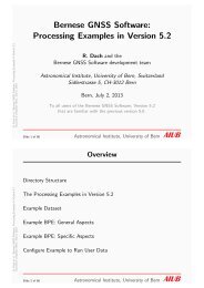
<strong>Bernese</strong> <strong>GNSS</strong> <strong>Software</strong><strong>Version</strong> <strong>5.2</strong><strong>Tutorial</strong>Processing ExampleIntroductory CourseTerminal SessionRolf Dach, Peter WalserJanuary 2014AIUBAstronomical Institute, University of Bern
1 Introduction to the Example Campaign1.1 Stations in the Example CampaignData from thirteen European stations of the International <strong>GNSS</strong> Service (IGS) networkand from the EUREF Permanent Network (EPN) were selected for the examplecampaign. They are listed in Table 1.1. The locations of these stations aregiven in Figure 1.1. Three of the stations support only Global Positioning System(GPS) whereas all other sites provide data from both GPS and its Russian counterpartGlobalьna navigacionna sputnikova sistema: Global Navigation Satellite System(GLONASS).The observations for these stations areavailable for four days. Two days in year2010 (day of year 207 and 208) and twoin 2011 (days 205 and 206). In the terminalsessions you will analyze the datain order to obtain a velocity field basedon final products from Center for OrbitDetermination in Europe (CODE). Foreight of these stations, coordinates andvelocities are given in the IGb08 referenceframe, an IGS–specific realizationof the ITRF2008 (see ${D}/STAT_LOG/IGb08.snx).Between these days in 2010 and 2011the receivers (LAMA, TLSE, WTZR) andthe full equipment (WTZZ) have beenchanged. The receiver type, the antennatype, and the antenna height are also providedin Table 1.1. Notice, that for threeantennas (GANP, WTZR, ZIM2) valuesfrom an individual calibration are availableTLSEWSRTONSAPTBBHERTWTZZWTZRZIM2ZIMMReceiver is trackingGPS/GLONASSMATELAMAJOZ2GANPStation with coordinates/velocities in IGb08GPS−onlyFigure 1.1: Stations used in example campaignfrom the EPN processing. For all other antennas only type–specific calibration resultsfrom the IGS processing (${X}/GEN/IGS08.ATX) are available. More details are providedin Table 1.2. Only in two cases where no calibration of the antenna/radome combinationwas available (ONSA, WSRT) the calibration values of the antenna without radome wereused instead. With one exception (ONSA) even system–specific calibrations for GPS andGLONASS measurements are available.The distances between stations in the network are between 200 and 1000 km. Thereare two pairs of receivers at one site included in the example dataset: in Zimmerwald,the distance between ZIMM and ZIM2 is only 19 m. In Kötzting the receivers WTZR,Page 1
1 Introduction to the Example CampaignTable 1.1: List of stations used for the example campaign including receiver and antenna typeas well as the antenna height.Receiver type AntennaStation name Location Antenna type Radome heightGANP11515M001 Ganovce, Slovakia TRIMBLE NETR8TRM55971.00 NONE 0.3830mHERT13212M010 Hailsham, LEICA GRX1200GGPROUnited Kingdom LEIAT504GG NONE 0.0000mJOZ212204M002 Jozefoslaw, PolandLAMA12209M001 Olsztyn, PolandMATE12734M008 Matera, ItalyONSA10402M004 Onsala, SwedenPTBB14234M001 Braunschweig, GermanyTLSE10003M009 Toulouse, FranceLEICA GRX1200GGPROLEIAT504GG NONE 0.0000m2010:LEICA GRX1200GGPROLEIAT504GG LEIS 0.0600m2011:LEICA GRX1200+<strong>GNSS</strong>LEIAT504GG LEIS 0.0600mLEICA GRX1200GGPROLEIAT504GG NONE 0.1010mJPS E_GGDAOAD/M_B OSOD 0.9950mASHTECH Z–XII3TASH700936E SNOW 0.0562m2010:TRIMBLE NETR5TRM59800.00 NONE 1.0530m2011:TRIMBLE NETR9TRM59800.00 NONE 1.0530mWSRT13506M005 Westerbork, AOA SNR–12 ACTThe Netherlands AOAD/M_T DUTD 0.3888mWTZR14201M010 Kötzting, GermanyWTZZ14201M014 Kötzting, GermanyZIM214001M008 Zimmerwald, SwitzerlandZIMM14001M004 Zimmerwald, Switzerland2010:LEICA GRX1200GGPROLEIAR25.R3 LEIT 0.0710m2011:LEICA GRX1200+<strong>GNSS</strong>LEIAR25.R3 LEIT 0.0710m2010:TPS E_GGDTPSCR3_GGD CONE 0.2150m2011:JAVAD TRE_G3TH DELTALEIAR25.R3 LEIT 0.0450mTRIMBLE NETR5TRM59800.00 NONE 0.0000mTRIMBLE NETRSTRM29659.00 NONE 0.0000mPage 2AIUB
1 Introduction to the Example Campaign1.2.1 The DATAPOOL Directory Structure (${D})Motivation for the DATAPOOL areaThe idea of the DATAPOOL area is to place local copies of external files somewhere on yourfilesystem. It has several advantages compared to downloading the data each time whenstarting the processing:• The files are downloaded only once, even if they are used for several campaigns.• The data download can be organized with a set of scripts running independently fromthe <strong>Bernese</strong> <strong>GNSS</strong> <strong>Software</strong> environment, scheduled by the expected availability ofthe external files to download.• The processing itself becomes independent from the availability of external datasources.Structure and content of the DATAPOOL areaThe DATAPOOL area contains several subdirectories taking into account the different potentialsources of files and their formats:RINEX :The data of <strong>GNSS</strong> stations is provided in Receiver INdependent EXchange format(RINEX) files. The directory contains observation (Hatanaka–compressed) andnavigation (GPS and GLONASS) files. These RINEX files are “originary” files thatare not changed during the processing.The RINEX files can be downloaded from international data centers. Project–specificfiles are copied into this area. If you mix the station lists from different projects,take care on the uniqueness of the four–character IDs of all stations in the RINEXfile names.HOURLY :The same as the RINEX directory but dedicated to hourly RINEX data as used fornear real–time applications. Note: not all stations in this example provide hourlyRINEX files.LEO :This directory is intended to host files which are necessary for Low Earth Orbiter(LEO) data processing. RINEX files are stored in the subdirectory RINEX (of the LEOdirectory). The corresponding attitude files are placed in the subdirectory ATTIT.These files are needed to run the example BPE on LEO orbit determination (LEOPOD.PCF). They are not used in the example during the <strong>Bernese</strong> Introductory Course.SLR_NP :The Satellite Laser Ranging (SLR) data is provided in the quicklook normal pointformat. The directory contains the normal point files downloaded from the InternationalLaser Ranging Service (ILRS) data centers.These files are needed to run the example BPE on validating orbit using SLR observations(SLRVAL.PCF). They are not used in the example during the <strong>Bernese</strong>Introductory Course.Page 4AIUB
1.2 Directory StructureSTAT_LOG :This directory contains the station information files (e.g., from ftp://igscb.igs.org/pub/station/general). This information may be completed by the originaryinformation on the reference frame (e.g., the IGb08.snx from ftp://igscb.igs.org/pub/station/coord).It also contains (apart from the coordinates and velocities of selected IGS sites)the history of the used equipment as it has been assumed for the reference framegeneration. A comparison with the igs.snx file constructed at the IGS CentralBureau (IGSCB) from the site information files may be useful for a verification ofthe history records.COD/IGS :Orbits, Earth orientation parmeters (EOP), and satellite clock corrections are basicexternal information for a <strong>GNSS</strong> analysis. The source of the files may be theFTP server from CODE (ftp://ftp.unibe.ch/aiub/CODE or http://www.aiub.unibe.ch/download/CODE/), or the Crustal Dynamics Data Information SystemFTP server (e.g., for downloading GPS–related IGS products ftp://cddis.gsfc.nasa.gov/gnss/products and in ftp://cddis.gsfc.nasa.gov/glonass/productsfor GLONASS–related IGS products). The files are named with the GPS week andthe day of the week (apart from files containing information for the entire week, e.g.,EOP, or the processing summaries).The IGS provides GPS and GLONASS orbits only in separate files (IGS/IGL–seriesfrom the final product line) stemming from independent combination procedureswith different contributing analysis center (AC). Nevertheless, they are consistentenough to merge both files together as the first step of the processing. CODEcontributes fully combined multi–<strong>GNSS</strong> solutions to the IGS final (and ultra–rapid)product line.BSW52 :In this directory we have placed files containing external input information in<strong>Bernese</strong>–specific formats. The files are neutral with respect to the data you aregoing to process. Typical examples are ionosphere maps or differential code biases(DCB) files. These files can be downloaded from http://www.aiub.unibe.ch/download/CODE/ or http://www.aiub.unibe.ch/download/BSWUSER52/ areas.REF52 :Here we propose to collect files in <strong>Bernese</strong> format which are useful for severalcampaigns (e.g., reference frame files: IGB08_R.CRD, IGB08_R.VEL). Typical examplesare station coordinate, velocity, and information files (e.g., EXAMPLE.CRD,EXAMPLE.VEL, EXAMPLE.STA, . . . , EPN.CRD). All stations of a project are containedin one file but the processing of the project’s data may be performed in differentcampaigns.MSC :This directory contains example files for the automated processing with the BPE.VMF1 :The grids for the Vienna Mapping Function (VMF1) are located in a separate directory.The files can be downloaded from http://ggosatm.hg.tuwien.ac.at/DELAY/GRID/VMFG/. They are not used for the examples but it shall indicate that for othertypes of files other directories may be created.<strong>Bernese</strong> <strong>GNSS</strong> <strong>Software</strong>, <strong>Version</strong> <strong>5.2</strong> Page 5
1 Introduction to the Example CampaignAll files and meta–information related to the 13 stations selected for the example campaignare already in this DATAPOOL–area (${D}) after installing the <strong>Bernese</strong> <strong>GNSS</strong> <strong>Software</strong>.<strong>GNSS</strong> orbit information is available from CODE and IGS (directory ${D}/COD or ${D}/IGS).1.2.2 The Campaign–Directory StructurePutting data from the DATAPOOL into the campaignWhen running an automated processing using the BPE there is a script at the beginningof the process which copies the data from the DATAPOOL–area into the campaign. If youare going to process data manually you first have to copy the necessary files into thecampaign and decompress them if necessary using standard utilities (uncompress,gunzip 1 ,or CRZ2RNX for RINEX–files).Content of the campaign area to process the exampleAll files needed to process the data according to this tutorial are already copied into thecampaign area. If you want to follow the example outside the <strong>Bernese</strong> Introductory Courseenvironment you have to put the following files at the correct places in the campaigndirectory structure.${P}/INTRO/ATM/ COD10207.ION COD10208.ION COD11205.ION COD11206.ION${P}/INTRO/BPE/${P}/INTRO/GRD/ VMF10207.GRD VMF10208.GRD VMF11205.GRD VMF11206.GRD${P}/INTRO/OBS/${P}/INTRO/ORB/ IGS15941.PRE IGS15942.PRE IGS16460.PRE IGS16461.PREIGL15941.PRE IGL15942.PRE IGL16460.PRE IGL16461.PREIGS15947.IEPIGS16467.IEPCOD15941.PRE COD15942.PRE COD16460.PRE COD16461.PRECOD15947.IEPCOD16467.IEPP1C11007.DCBP1C11107.DCBP1P21007.DCBP1P21107.DCB${P}/INTRO/ORX/${P}/INTRO/OUT/ IGS15941.CLK IGS15942.CLK IGS16460.CLK IGS16461.CLKCOD15941.CLK COD15942.CLK COD16460.CLK COD16461.CLK${P}/INTRO/RAW/ GANP2070.10O GANP2080.10O GANP2050.11O GANP2060.11OHERT2070.10O HERT2080.10O HERT2050.11O HERT2060.11OJOZ22070.10O JOZ22080.10O JOZ22050.11O JOZ22060.11OLAMA2070.10O LAMA2080.10O LAMA2050.11O LAMA2060.11OMATE2070.10O MATE2080.10O MATE2050.11O MATE2060.11OONSA2070.10O ONSA2080.10O ONSA2050.11O ONSA2060.11OPTBB2070.10O PTBB2080.10O PTBB2050.11O PTBB2060.11OTLSE2070.10O TLSE2080.10O TLSE2050.11O TLSE2060.11OWSRT2070.10O WSRT2080.10O WSRT2050.11O WSRT2060.11OWTZR2070.10O WTZR2080.10O WTZR2050.11O WTZR2060.11OWTZZ2070.10O WTZZ2080.10O WTZZ2050.11O WTZZ2060.11OZIM22070.10O ZIM22080.10O ZIM22050.11O ZIM22060.11OZIMM2070.10O ZIMM2080.10O ZIMM2050.11O ZIMM2060.11O${P}/INTRO/SOL/${P}/INTRO/STA/ EXAMPLE.CRD EXAMPLE.VEL EXAMPLE.STA EXAMPLE.ABBEXAMPLE.BLQ EXAMPLE.ATL EXAMPLE.CLU EXAMPLE.PLDIGB08_R.CRD IGB08_R.VEL IGB08.FIX IGB08.SIGSESSIONS.SES1 These tools are also available for WINDOWS-platforms, see www.gzip.org. Note, that gunzip can alsobe used to uncompress UNIX–compressed files with the extension .Z.Page 6AIUB
1.2 Directory StructureThe directory${P}/INTRO/GEN/ contains copies of files from the${X}/GEN directory, whichare used by the processing programs. If you want to view these files, please use those in yourcampaign and not the ones in the ${X}/GEN directory to prevent potential interferenceswith your colleagues.${P}/INTRO/GEN/ CONST. DATUM. GPSUTC. POLOFF.RECEIVER.SATELLIT.I08 PCV.I08 I08.ATXSAT_2010.CRX SAT_2011.CRXIAU2000R06.NUT IERS2010XY.SUB OT_FES2004.TID TIDE2000.TPOEGM2008_SMALL. s1_s2_def_ce.datSINEX. SINEX.PPP SINEX.RNX2SNXIONEX. IONEX.PPP1.2.3 Input Files for the Processing ExamplesAtmosphere files ATMThe input files in this directory are global ionosphere models in the <strong>Bernese</strong> format obtainedfrom the IGS processing at CODE. They will be used to support the phase ambiguityresolution with the QIF strategy and to enable the higher order ionosphere (HOI)corrections.General files GENThese general input files contain information that is neither user– nor campaign–specific.They are accessed by all users, and changes in these files will affect processing for everyone.Consequently, these files are located in the ${X}/GEN directory. Table 1.3 shows the listof general files necessary for the processing example. It also shows which files need to beupdated from time to time by downloading them from the anonymous ftp–server of AIUB(http://www.aiub.unibe.ch/download/BSWUSER52/GEN).Each <strong>Bernese</strong> processing program has its own panel for general files. Make sure that youuse the correct files listed in Table 1.3 .Grid files GRDIn this directory the grid files *.GRD are collected. To apply for instance the VMF1 tropospheremodel (a priori information from European Centre for Medium-Range WeatherForecasts (ECMWF) and Vienna mapping function) you need a grid with the necessarycoefficients.Orbit files ORBThe precise orbits in the files *.PRE are usually the final products from CODE analysiscenter containing GPS and GLONASS orbits from a rigorous multi–<strong>GNSS</strong> analysis. Alternativelyalso the combined final products from the IGS can be used. They do not containorbits for the GLONASS satellites. The combined GLONASS satellite orbits from the IGSare available in IGL–files. Both precise orbit files need to be merged for a multi–<strong>GNSS</strong>analysis.The corresponding EOP are given in weekly files with the extension *.IEP (takecare on full consistency with the orbit product).Furthermore, the directory contains monthly means for the DCB.<strong>Bernese</strong> <strong>GNSS</strong> <strong>Software</strong>, <strong>Version</strong> <strong>5.2</strong> Page 7
1 Introduction to the Example CampaignTable 1.3: List of general files to be used in the <strong>Bernese</strong> programs for the processing example.Filename Content Modification Update fromCONST. All constants used in the NoBSW aftp<strong>Bernese</strong> <strong>GNSS</strong> <strong>Software</strong>DATUM. Definition of geodetic Introducing new reference BSW aftpdatumellipsoidGPSUTC. Leap seconds When a new leap second is BSW aftpannounced by the IERSPOLOFF. Pole offset coefficients Introducing new values —from IERS annual report(until 1997)RECEIVER. Receiver information Introducing new receiver BSW aftptypeSATELLIT.I08 Satellite information file New launched satellites BSW aftpPCV.I08 Phase center eccentricities Introducing new antenna BSW aftp orand variationscorrections or new update withantenna/radome ATX2PCVcombinationsSAT_$Y+0.CRX Satellite problems Satellite maneuvers, bad BSW aftpdata, ...IAU2000R06.NUT Nutation model No —coefficientsIERS2010XY.SUB Subdaily pole model No —coefficientsOT_FES2004.TID Ocean tides coefficients No —TIDE2000.TPO Solid Earth tides No —coefficientsEGM2008_SMALL. Earth potential coefficients No —(reduced version, sufficientfor <strong>GNSS</strong> and LEO orbitdetermination)s1_s2_def_ce. S1/S2 atmospheric tidal No —datloading coefficientsSINEX. SINEX header information Adapt SINEX header for —SINEX.TROyour institutionSINEX.PPP ...for the PPP exampleSINEX.RNX2SNX ...for RNX2SNX exampleIONEX. IONEX header Adapt IONEX header for —informationyour institutionIONEX.PPP ...for the PPP examplePage 8AIUB
1.2 Directory StructureClock RINEX files OUTThe clock RINEX files are located in the OUT–directory. They are consistent withthe <strong>GNSS</strong> orbits and EOP products in the ORB–directory. They contain station andsatellite clock corrections with at least 5 minutes sampling — there are also files fromthe IGS or some of the ACs providing satellite clock corrections with a sampling of30 seconds.RINEX files RAWThe raw data are given in RINEX format. The observations *.$YO ($Y is the menutime variable for the two–digit year of the current session) are used for all examples.Station files STAThe coordinates and velocities of the stations given in the IGS realization of the referenceframe ITRF2008 are available in the files IGB08_R.CRD and IGB08_R.VEL. The IGS corestations are listed in IGB08.FIX. This file will be used to define the geodetic datum whenestimating station coordinates. You can browse all these files with a text editor or withthe menu ("Menu>Campaign>Edit station files").For all stations that have unknown coordinates in the IGb08 reference frame a PrecisePoint Positioning (PPP) using the example BPE (PPP_BAS.PCF) for day 207 of year 2010has been executed. For our EXAMPLE–project a resulting coordinate file EXAMPLE.CRD hasbeen generated. It contains all IGS core sites (copied from file IGB08_R.CRD) and thePPP results for the remaining stations. The epoch of the coordinates is January 01,2005. The corresponding velocity file EXAMPLE.VEL contains the velocities for the coresites (copied from file IGB08_R.VEL) completed by the NNR–NUVEL1A velocities for theother stations. The assignment of stations to tectonic plates is given in the file EXAMPLE.PLD.To make sure that you process the data in the <strong>Bernese</strong> <strong>GNSS</strong> <strong>Software</strong> with correctstation information (station name, receiver type, antenna type, antenna height, etc.) thefile EXAMPLE.STA is used to verify the RINEX header information. The reason to use thisfile has to be seen in the context that some antenna heights or receiver/antenna types inthe RINEX files may not be correct or may be measured to a different antenna referencepoint. Similarly, the marker (station) names in the RINEX files may differ from the nameswe want to use in the processing. The antenna types have to correspond to those in thefile ${X}/GEN/PCV.I08 in order that the correct phase center offsets and variations areused. The receiver types have to be defined in the ${X}/GEN/RECEIVER. file to correctlyapply the DCB corrections.For each station name unique four– and two–character abbreviations to construct thenames for the <strong>Bernese</strong> observation files need to be defined in the file EXAMPLE.ABB. It wasautomatically generated by the PPP–example BPE. If you want to process big networks,the baselines need to be divided into clusters to speed up the processing. For that purposeeach station has to be assigned to a region by a cluster number in the file EXAMPLE.CLU.<strong>Bernese</strong> <strong>GNSS</strong> <strong>Software</strong>, <strong>Version</strong> <strong>5.2</strong> Page 9
1 Introduction to the Example CampaignThe last files to be mentioned in this directory are EXAMPLE.BLQ and EXAMPLE.ATL. Theyrespectively provide the coefficients for the ocean and atmospheric tidal loading of thestations. They should at least be applied in the final run of GPSEST.1.2.4 The SAVEDISK Directory Structure (${S})Motivation for the SAVEDISK areaWhen processing <strong>GNSS</strong> data, a lot of files from various processing steps will populateyour campaign directories. The main result files from the data analysis should be collectedin the SAVEDISK area. This area is intended as long–term archive for your resultfiles.Because the result files are stored in the SAVEDISK area, you can easily clean up your campaignarea without loosing important files. Please keep in mind that the computing performancedecreases if you have several thousands of files in a directory.Structure and content of the SAVEDISK areaWe propose to build subdirectories in the SAVEDISK area for each of your projects. If theseprojects collect data over several years, yearly subdirectories are recommended. It is alsopractical to use further subdirectories like ATM, ORB, OUT, SOL, STA to distribute the filesand to get shorter listings if you are looking for a file.The SAVEDISK area contains after its installation a directory structure according to thedescription above. Each example BPE is assumed as a project. Therefore, you will find onthe top level of the SAVEDISK the directories PPP, RNX2SNX, CLKDET, LEOPOD, and SLRVAL(related to the different example BPEs).In each of these directories you will find several files ending with _REF. They are generatedby running the example BPEs on the system at Astronomical Institute of theUniversity of Bern (AIUB). Even if the objectives of this tutorial and of the RNX2SNXexample BPE are in both cases to process data from a regional network, the resuls mustnot be identical since there are some differences in the processing strategies and selectedoptions.Page 10AIUB
2 Terminal Session: MondayToday’s terminal session is to:1. become familiar with the UNIX environment, the menu of the <strong>Bernese</strong> <strong>GNSS</strong><strong>Software</strong>, and the example campaign,2. verify the campaign setup done for you (see sections 2.2 and 2.3, and alsothe handout for the terminal sessions),3. generate the a priori coordinates for all 4 days using COOVEL (see Section2.5), and4. start to prepare pole and orbit information according to chapter 3.2.1 Start the MenuStart the menu program using the command G 1 .Navigate through the submenus to become familiar with the structure of the menu. Readthe general help (available at "Menu>Help>General") to get an overview on the usage of themenu program of the <strong>Bernese</strong> <strong>GNSS</strong> <strong>Software</strong>.For the terminal session in the <strong>Bernese</strong> Introductory Course, the campaign setup hasalready been done for each user. Please check that the campaign name in the statusbarof the <strong>Bernese</strong> Menu is set correctly to your campaign (i.e., Campaign ${P}/INTRO) andthat the current session is set to the first session (i.e., $Y+0=2010, $S+0=2070). If thisis not the case, please contact the staff in the Terminal room.2.2 Select Current SessionSelect "Menu>Campaign>Edit session table" to check the session table. It is recommended to usethe wildcard string ???0 for the “List of sessions” in panel “SESSION TABLE”. The panel belowshows the session definition for a typical permanent campaign with 24-hours sessions. Thesetup of the session table is a very important task when you prepare a campaign. Pleaseread the corresponding online help carefully.1 At the exercise terminals the <strong>Bernese</strong> environment is loaded automatically during the login. At homeyou have to source the file ${X}/EXE/LOADGPS.setvar on UNIX–platforms either manually or duringthe login.Page 11
2 Terminal Session: MondaySave the session table (press the ˆSave button) and open the “Date Selection Dialog”in the "Menu>Configure>Set session/compute date" in order to define the current session:2.3 Campaign SetupUsually, a new campaign must be added to the campaign list ("Menu>Campaign>Edit list ofcampaigns") first and select it as the active campaign ("Menu>Campaign>Select active campaign"),before the directory structure can be created ("Menu>Campaign>Create new campaign"). In the<strong>Bernese</strong> Introductory Course environment this should already have been done for yourcampaign, but please verify that.In the <strong>Bernese</strong> Introductory Course environment the selected campaign should be ${P}/INTRO. In order to become familiar with the campaign structure, you can inspect yourcampaign directory and inspect the contents using the command line (using cd for changingdirectories and ls to create directory listings) or using a filemanager (e.g., midnightcommander mc).2.4 Menu VariablesWhen processing <strong>GNSS</strong> data, it is often necessary to repeat a program run several timeswith only slightly different option settings. A typical example would be the processingof several sessions of data. The names of observation files change from session to sessionbecause the session number is typically a part of the filename. It would be verycumbersome to repeat all the runs selecting the correct files manually every time. Forthe BPE an automation is mandatory. For such cases the <strong>Bernese</strong> menu system providesa powerful tool: the so–called menu variables. The menu variables are defined inthe user–specific menu input file ${U}/PAN/MENU_VAR.INP that is accessible through "MenuPage 12AIUB
2.4 Menu Variables>Configure>Menu variables". Three kinds of menu variables are available: predefined variables(also called menu time variables), user–defined variables, and system environment variables.The use of system environment variables is necessary to generate the complete path tothe files used in the <strong>Bernese</strong> <strong>GNSS</strong> <strong>Software</strong>. The campaign data are located in thedirectory ${P}/INTRO=${HOME}/GPSDATA/INTRO. The user–dependent files can be foundat ${U}=${HOME}/GPSUSER52 — note that ${HOME} may have been already translated intothe name of your home–directory. The temporary user files are saved in ${T}=/scratch/local/bern52. Finally, the campaign–independent files reside in ${X}=/home/bswadmin/BERN52/GPS.The predefined variables provide a set of time strings assigned to the current session. Fromthe second panel of the menu variables you get an overview on the available variables andtheir usage:Be aware that the variable $S+1 refers to the next session. Because we are using a sessiontable for daily processing it also corresponds to the next day.<strong>Bernese</strong> <strong>GNSS</strong> <strong>Software</strong>, <strong>Version</strong> <strong>5.2</strong> Page 13
2 Terminal Session: MondayThese variables are automatically translated by the menu upon saving the panel or runningthe program. We recommend to make use of them in the input panels (e.g. for filenamespecification).2.5 Generate A Priori CoordinatesAs stated before the a priori coordinates generated from the PPP processing example BPErefer to the epoch January 01, 2005 . The first step is to extrapolate the coordinates to theepoch that is currently processed. This is the task of the program COOVEL. Open the programinput panel in "Menu>Service>Coordinate tools>Extrapolate coordinates":“Reference epoch: date” $YMD_STR+0 → 2010 07 26“Output coordinate file” APR$YD+0 → APR10207“Title line” Session $YSS+0: → Session 102070:Start the program with the ˆRun–button. The program generates an output file COOVEL.L?? in the directory ${P}/INTRO/OUT. This file may be browsed using the ˆOutput–buttonor with "Menu>Service>Browse program output". It should look like===============================================================================<strong>Bernese</strong> <strong>GNSS</strong> <strong>Software</strong>, <strong>Version</strong> <strong>5.2</strong>-------------------------------------------------------------------------------Program : COOVELPurpose : Extrapolate coordinates-------------------------------------------------------------------------------Campaign : ${P}/INTRODefault session: 2070 year 2010Date : 10-Jan-2014 16:27:03User name : bern52===============================================================================EXAMPLE: Session 102070: Coordinate propagation-------------------------------------------------------------------------------Page 14AIUB
2.5 Generate A Priori CoordinatesINPUT AND OUTPUT FILENAMES---------------------------------------------------------------------------------------------------------Input coordinate file : ${P}/INTRO/STA/EXAMPLE.CRDInput velocity file : ${P}/INTRO/STA/EXAMPLE.VELOutput coordinate file : ${P}/INTRO/STA/APR10207.CRDProgram output: ${P}/INTRO/OUT/COOVEL.L00Error message: ${U}/WORK/ERROR.MSGSession table: ${P}/INTRO/STA/SESSIONS.SES-------------------------------------------------------------------------------REFERENCE EPOCH: 2005-01-01 00:00:00INTERPOLATION FACTOR: -5.563312799452429NO 15 -VELOCITY: ASPA%50503S006NO 49 -VELOCITY: CONZ%41719M002NO 153 -VELOCITY: MQZG%50214M001NO 156 -VELOCITY: MTKA%21741S002NO 207 -VELOCITY: SANT%41705M003NO 243 -VELOCITY: TSKB%21730S005----------------------------------------------------------------->>> CPU/Real time for pgm "COOVEL": 0:00:00.013 / 0:00:00.013>>> Program finished successfullyThe header area of the program output is standardized for all programs of the <strong>Bernese</strong><strong>GNSS</strong> <strong>Software</strong>, <strong>Version</strong> <strong>5.2</strong> . Furthermore each program has a title line that shouldcharacterize the program run. It is printed to the program output and to most of theresult files. Many program output files furthermore provide a list of input and output filesthat have been used or generated.The last two lines of the above example appear also in each program output of the <strong>Bernese</strong><strong>GNSS</strong> <strong>Software</strong>, <strong>Version</strong> <strong>5.2</strong>. It reports the processing time and the status successful orwith error.There are a number of stations with coordinates but no velocities (indicated in the programoutput as NO 15 -VELOCITY: ASPA%50503S006). The coordinates cannot be used asfiducial point for datum definition mostly because of earthquake events. We have none ofthese stations in our example.The result of the run of COOVEL is an a priori coordinate file (${P}/INTRO/STA/APR10207.CRD) containing the positions of the sites to be processed for the epoch of the current session(the lines for the other stations are ignored in the processing):EXAMPLE: Session 102070: Coordinate propagation--------------------------------------------------------------------------------LOCAL GEODETIC DATUM: IGb08 EPOCH: 2010-07-26 00:00:00NUM STATION NAME X (M) Y (M) Z (M) FLAG71 GANP 11515M001 3929181.41960 1455236.82354 4793653.94456 P89 HERT 13212M010 4033460.85011 23537.89173 4924318.31616 I106 JOZ2 12204M002 3664880.47637 1409190.67771 5009618.53053 I123 LAMA 12209M001 3524522.83219 1329693.71146 5129846.40491 P136 MATE 12734M008 4641949.45506 1393045.52839 4133287.55041 I174 ONSA 10402M004 3370658.46283 711877.21896 5349787.00996 I193 PTBB 14234M001 3844059.87356 709661.40870 5023129.60550 P236 TLSE 10003M009 4627851.76560 119640.12481 4372993.62094 I258 WSRT 13506M005 3828735.77808 443305.04589 5064884.76561 I259 WTZR 14201M010 4075580.45801 931853.89288 4801568.18631 I260 WTZZ 14201M014 4075579.32680 931853.20354 4801569.09338 P270 ZIM2 14001M008 4331299.79229 567537.42322 4633133.79466 P272 ZIMM 14001M004 4331296.98900 567555.97843 4633134.00316 IRepeat this step for the other three sessions of the example by changing the currentsession using the ˆ+Day or ˆ-Day to change a limited number of days (not sessions) or via"Menu>Configure>Set session/compute date" . You can then use the Rerˆun button to restart theprogram. No options need to be changed because of the consequent use of the menu timevariables was made.<strong>Bernese</strong> <strong>GNSS</strong> <strong>Software</strong>, <strong>Version</strong> <strong>5.2</strong> Page 15
2 Terminal Session: Monday2.6 Session GoalsAt the end of this session, you should have created the following files:1. a priori coordinates in your campaign’s STA directory: files APR10207.CRD,APR10208.CRD, ...These files must be generated for all four days (days 207 and 208 of year2010 and days 205 and 206 of year 2011).Until the end of the Monday’s terminal session you should start with preparingthe pole and orbit information, see Chapter 3.Page 16AIUB
3 Terminal Session: Pole and OrbitPreparation (Monday/Tuesday)The terminal session on pole and orbit preparation is to:1. generate the pole information file in the <strong>Bernese</strong> format (POLUPD)2. generate tabular orbit files from CODE precise files (PRETAB)3. generate the <strong>Bernese</strong> standard orbit files (ORBGEN)You should start with these tasks during the Monday’s terminal sessions and finishthe processing during the terminal session on Tuesday.Introductory RemarkWe recommend to use the final or preprocessed products from CODE because they containconsistent orbits for GPS and GLONASS. They also include all active <strong>GNSS</strong> satellites(even if they are unhealthy or during GPS satellite repositioning events) with thehighest possible accuracy thanks to three–day long–arc technology. Due to this choiceyou will get the best possible consistency between the external products and the software.You may alternativly use the products from IGS. Seperate product files for GPS andGLONASS orbits exist from independent combination procedures that first need to bemerged for a multi–<strong>GNSS</strong> processing. For most of the applications, merging the preciseorbit files is sufficient — a tutorial on the procedure is given in Sect. 7.1 of this book.On the other hand, the consistency of the orbits can not be as good as that of CODE (orother analysis center) following the strategy of the rigorous combined processing of GPSand GLONASS measurements for orbit determination.3.1 Prepare Pole InformationTogether with the precise orbit files (PRE), a consistent set of Earth orientation informationis provided in the ORB directory. Whereas the orbits are given in daily files the EOP areavailable in weekly files for the final product series from the CODE analysis center. Wehave to convert the information from the International Earth Rotation and ReferenceSystems Service (IERS)/IGS standard format (file extension within the <strong>Bernese</strong> <strong>GNSS</strong><strong>Software</strong> is IEP) into the internal <strong>Bernese</strong> EOP format (file extension within the <strong>Bernese</strong><strong>GNSS</strong> <strong>Software</strong> is ERP). This is the task of the program POLUPD ("Menu>Orbits/EOP>HandleEOP files>Convert IERS to <strong>Bernese</strong> Format") which is also able to update the EOP records of anexisting file.Page 17
3.2 Generate Orbit FilesThe last panel for the program POLUPD is an example for the specification of time windowsin the <strong>Bernese</strong> <strong>GNSS</strong> <strong>Software</strong>, <strong>Version</strong> <strong>5.2</strong>. Time windows can be defined by sessions(a single session or a range of sessions). Alternatively, a time window may be specifiedby a start and an end epoch. By entering either a start or an end epoch you may defineonly the beginning or the end of the time interval. We refer to the online help for moredetails.The messages### PG POLUPD: NUTATION MODEL NAME NOT EQUAL DEFAULTDEFAULT NUTATION MODEL NAME : IAU2000R06NUTATION MODEL NAME IN FILE : IAU2000### PG POLUPD: SUBDAILY POLE MODEL NAME NOT EQUAL DEFAULTDEFAULT SUBDAILY POLE MODEL NAME : IERS2010SUBDAILY POLE MODEL NAME IN FILE : IERS2000just inform that you have selected the most recent nutation and subdaily pole modelwhereas the operational solution at CODE was computed using an older model at thattime.If you do not want to accept this inconsistency you may alternatively use the resultsfrom a reprocessing effort (e.g., http://www.aiub.unibe.ch/download/REPRO_2011/CODE/).3.2 Generate Orbit FilesIn this processing example we use only two programs of the orbit part of the <strong>Bernese</strong><strong>GNSS</strong> <strong>Software</strong>. The first program is called PRETAB and may be accessed using "Menu>Orbits/EOP>Create tabular orbits". The main task of PRETAB is to create tabular orbit files(TAB) (i.e., to transform the precise orbits from the terrestrial into the celestial referenceframe) and to generate a satellite clock file (CLK). The clock file will be needed, e.g.,in a program CODSPP (see Section 4.2.1, to be discussed in the Tuesday’s lectures onpre-processing).<strong>Bernese</strong> <strong>GNSS</strong> <strong>Software</strong>, <strong>Version</strong> <strong>5.2</strong> Page 19
3 Terminal Session: Pole and Orbit PreparationYou have to apply the same subdaily pole and nutation models as you have used beforewhen you have generated the <strong>Bernese</strong> formatted pole file (IGS$YD+0.ERP).If you process precise orbits from CODE it is generally not necessary to remove badsatellites. It might become necessary for orbit products from other sources (e.g., from theIGS). Because CODE introduces the correct accuracy code for all its satellites the abovesettings do not harm the import of satellite orbits from CODE.Panel “PRETAB 3: Options for Clocks” contains the options for extracting the satellite clockinformation. The clock values in the precise orbit file are sampled to 15 min. We interpolatewith a “Polynomial degree” of 2 with an “Interval for polynomials” of 12 hours. This is goodenough for the receiver clock synchronization in CODSPP.A message like this is expected:### PG PRETAB: SATELLITE CLOCK VALUES MISSINGSATELLITE : 101FILE NUMBER: 1FILE NAME : ${P}/INTRO/ORB/COD15951.PREPage 20AIUB
3.2 Generate Orbit Files### PG PRETAB: SATELLITE CLOCK VALUES MISSINGSATELLITE : 102FILE NUMBER: 1FILE NAME : ${P}/INTRO/ORB/COD15951.PRE...It indicates that the precise orbit files do not contain clock corrections for theGLONASS satellites (GLONASS satellite are indicated with satellite number between100 and 199 within the <strong>Bernese</strong> <strong>GNSS</strong> <strong>Software</strong>). Consequently the synchronizationof the receiver clocks in CODSPP will only be done based on the GPS satelliteclocks.The second program of the orbit part used here is called ORBGEN ("Menu>Orbits/EOP>Create/update standard orbits"). It prepares the so–called standard orbits using the satellitepositions in the tabular orbit files as pseudo–observations for a least–squares adjustment.Make sure that the ERP file, the nutation, and the subdaily pole model are the same youhave used in PRETAB. It is mandatory to consistently use this triplet of files together withthe generated standard orbits for all processing programs (otherwise a warning message isissued).<strong>Bernese</strong> <strong>GNSS</strong> <strong>Software</strong>, <strong>Version</strong> <strong>5.2</strong> Page 21
3 Terminal Session: Pole and Orbit PreparationPage 22AIUB
3.2 Generate Orbit FilesThe program produces an output file ORB10207.OUT (or corresponding to the other sessions)which should look like...INPUT AND OUTPUT FILENAMES---------------------------------------------------------------------------------------------------------General constants : ${X}/GEN/CONST.Correction GPS-UTC : ${X}/GEN/GPSUTC.Planetary ephemeris file : ${X}/GEN/DE405.EPHCoeff. of Earth potential : ${X}/GEN/EGM2008_SMALL.Solid Earth tides file : ${X}/GEN/TIDE2000.TPOOcean tides file : ${X}/GEN/OT_FES2004.TIDSatellite problems : ${X}/GEN/SAT_2010.CRXSatellite information : ${X}/GEN/SATELLIT.I08Nutation model: ${X}/GEN/IAU2000R06.NUTSubdaily pole model : ${X}/GEN/IERS2010XY.SUBPole file: ${P}/INTRO/ORB/COD10207.ERPOcean loading corrections : ${P}/INTRO/STA/EXAMPLE.BLQAtmospheric loading corrections : ${P}/INTRO/STA/EXAMPLE.ATLOrbital elements, file 1 : ---Orbital elements, file 2 : ---Standard orbits: ${P}/INTRO/ORB/COD10207.STDRadiation pressure coeff. : ---Summary file : ---Summary file for IGS-ACC : ${P}/INTRO/OUT/ORB10207.LSTResidual plot file : ---Residual file : ---Program output: ${P}/INTRO/OUT/ORB10207.OUTError message: ${U}/WORK/ERROR.MSGScratch file: ${U}/WORK/ORBGEN.SCRScratch file: ${U}/WORK/ORBGEN.SC2Session table: ${P}/INTRO/STA/SESSIONS.SES-------------------------------------------------------------------------------...<strong>Bernese</strong> <strong>GNSS</strong> <strong>Software</strong>, <strong>Version</strong> <strong>5.2</strong> Page 23
3 Terminal Session: Pole and Orbit Preparation...-------------------------------------------------------------------------------RMS ERRORS AND MAX. RESIDUALS ARC NUMBER: 1 ITERATION: 4-------------------------------------------------------------------------------QUADRATIC MEAN OF O-C (M) MAX. RESIDUALS (M)SAT #POS RMS (M) TOTAL RADIAL ALONG OUT RADIAL ALONG OUT--- ---- ------- ----------------------------- --------------------1 96 0.001 0.001 0.001 0.001 0.001 0.002 0.003 0.0022 96 0.001 0.001 0.000 0.001 0.001 0.001 0.002 0.0023 96 0.001 0.001 0.001 0.001 0.001 0.003 0.003 0.0024 96 0.001 0.001 0.001 0.001 0.001 0.001 0.002 0.0025 96 0.001 0.001 0.001 0.001 0.001 0.002 0.003 0.0036 96 0.001 0.001 0.001 0.001 0.001 0.002 0.003 0.0027 96 0.001 0.001 0.001 0.001 0.001 0.002 0.003 0.0038 96 0.001 0.001 0.001 0.001 0.001 0.003 0.003 0.0039 96 0.001 0.001 0.001 0.001 0.001 0.002 0.004 0.00210 96 0.001 0.001 0.001 0.001 0.001 0.001 0.002 0.00211 96 0.001 0.001 0.001 0.001 0.001 0.002 0.003 0.00212 96 0.001 0.001 0.001 0.001 0.001 0.002 0.003 0.00213 96 0.001 0.001 0.001 0.001 0.001 0.002 0.003 0.002...28 96 0.001 0.001 0.001 0.001 0.001 0.002 0.003 0.00229 96 0.001 0.001 0.001 0.001 0.001 0.002 0.002 0.00130 96 0.001 0.001 0.001 0.001 0.001 0.003 0.003 0.00231 96 0.001 0.001 0.001 0.001 0.001 0.002 0.003 0.00232 96 0.001 0.001 0.001 0.001 0.001 0.003 0.003 0.002101 96 0.001 0.001 0.001 0.001 0.001 0.002 0.002 0.002102 96 0.001 0.001 0.001 0.001 0.001 0.002 0.003 0.003103 96 0.001 0.001 0.001 0.001 0.001 0.002 0.003 0.002104 96 0.001 0.001 0.001 0.001 0.001 0.002 0.003 0.003105 96 0.001 0.001 0.001 0.001 0.001 0.001 0.003 0.002107 96 0.001 0.001 0.001 0.001 0.001 0.002 0.003 0.002...121 96 0.001 0.001 0.001 0.001 0.001 0.002 0.003 0.002122 96 0.001 0.001 0.001 0.001 0.001 0.002 0.003 0.002123 96 0.001 0.001 0.001 0.001 0.001 0.001 0.002 0.002124 96 0.001 0.001 0.001 0.001 0.001 0.001 0.003 0.002-------------------------------------------------------------------------------...The most important information in the output file are the RMS errors for each satellite.These should be 1 mm (for older orbits it may also achieve 3. . . 5 mm) if preciseorbits from CODE were used together with the consistent EOP information (theactual RMS errors depend on the quality of the precise orbits, on the pole file usedfor the transformation between IERS Terrestrial Reference Frame (ITRF) and InternationalCelestial Reference Frame (ICRF) in PRETAB, and on the orbit model used inORBGEN).Comparing the RMS error from the third and the fourth iteration you will see that threeiterations should already be enough to produce precise standard orbits for <strong>GNSS</strong> satellites.The file${P}/INTRO/OUT/ORB10207.LST summarizes the orbit fit RMS values in one table:EXAMPLE: Session 102070: Standard orbit generation 10-JAN-14 17:44TIME FROM DAY : 1 GPS WEEK: 1594TO DAY : 2 GPS WEEK: 1594-------------------------------------------------------------------------------ORBIT REPEATABILITY FROM A 1-DAY FIT THROUGH DAILY ORBIT SOLUTIONS (MM)# ECLIPSING SATELLITES: 5 E / 0 M ( 0 EM)----------------------------- ... ---------------------- ... ---------------------------- ...ECL .. .. .. .. .. .. .. E. E. E. .. .. .. .. .. .. .. ..DOY 1 2 3 4 5 6 ... 12 13 14 15 16 ... 32 101 102 103 104 105 107 ...----------------------------- ... ---------------------- ... ---------------------------- ...207 1 1 1 1 1 1 ... 1 1 1 1 1 ... 1 1 1 1 1 1 1 ...----------------------------- ... ---------------------- ... ---------------------------- ...ALL 1 1 1 1 1 1 ... 1 1 1 1 1 ... 1 1 1 1 1 1 1 ...----------------------------- ... ---------------------- ... ---------------------------- ...The output shows that 5 satellites are in eclipse (indicated above the satellite number byE for Earth or M for Moon).Page 24AIUB
3.3 Session GoalsThe similar file may be generated using the orbit products from IGS (including the EOPinformation) following the procedure described in Section 7.1 . As you can notice the RMSerrors are slightly higher. It does not mean that the orbits from CODE are better thanthe IGS orbits. The orbit model in ORBGEN is only more consistent with the orbit modelused at CODE:EXAMPLE: Session 102070: Standard orbit generation 10-JAN-14 18:28TIME FROM DAY : 1 GPS WEEK: 1594TO DAY : 2 GPS WEEK: 1594-------------------------------------------------------------------------------ORBIT REPEATABILITY FROM A 1-DAY FIT THROUGH DAILY ORBIT SOLUTIONS (MM)# ECLIPSING SATELLITES: 5 E / 0 M ( 0 EM)----------------------------- ... ---------------------- ... ----ECL .. .. .. .. .. .. .. E. E. E. .. ..DOY 1 2 3 4 5 6 ... 12 13 14 15 16 ... 32----------------------------- ... ---------------------- ... ----207 2 1 4 1 2 3 ... 3 3 3 2 3 ... 2----------------------------- ... ---------------------- ... ----ALL 2 1 4 1 2 3 ... 3 3 3 2 3 ... 2----------------------------- ... ---------------------- ... ----(Note the missing GLONASS satellites in the IGS orbit product.)In the example for day 208 of year 2010 a satellite 75 appears. The GPS–satellite 25 hada repositioning event at 2010–07–27 16:08:03 (see ${X}/GEN/SAT_2010.CRX). The satelliteis introduced in the processing with two independent arcs: one before (number 25) andone after (number 75) the event (you may verify this by the number of epochs availablefor each of these two satellite arcs).3.3 Session GoalsAt the end of this session, you should have created the following files:1. <strong>Bernese</strong> pole file in the campaign’s ORB directory: COD10207.ERP,2. <strong>Bernese</strong> standard orbit file in the ORB directory: COD10207.STD,3. <strong>Bernese</strong> satellite clock file in the ORB directory: COD10207.CLK.<strong>Bernese</strong> <strong>GNSS</strong> <strong>Software</strong>, <strong>Version</strong> <strong>5.2</strong> Page 25
3 Terminal Session: Pole and Orbit PreparationPage 26AIUB
4 Terminal Session: TuesdayToday’s terminal session is to:1. import the observations from the RINEX format into the <strong>Bernese</strong> formatfor all four days of the example using RXOBV3 (section 4.1).2. preprocess the <strong>Bernese</strong> observation files:• receiver clock synchronization (CODSPP, section 4.2.1)• baseline generation (SNGDIF, section 4.2.2)• preprocess baselines (MAUPRP, section 4.2.3)4.1 Importing the ObservationsThe campaign has now been set up and all necessary files are available. The first partof processing consists of the transfer of the observations from RINEX to <strong>Bernese</strong> (binary)format. To get an overview of the data availability you may generate a pseudographicfrom the RINEX observation files using the program RNXGRA in "Menu>RINEX>RINEX utilities>Create observation statistics" — this step is not mandatory but it may be usefulto get an impression of the tracking performance of the stations before you start theanalysis.Importing the RINEX observation files is the task of the program RXOBV3 in "Menu>RINEX>Import RINEX to <strong>Bernese</strong> format>Observation files" (we do not use the RINEX navigation files forthis processing example).All RINEX observation files fitting the pattern ${P}/INTRO/RAW/????2070.10O are selectedautomatically by the current entry in the input field “original RINEX observation files”.Page 27
4 Terminal Session: TuesdayYou can verify this by pressing the button just right from this input field (labeled with thefile extension 10O). In the file selection dialog you will find the list of currently selectedfiles. The RINEX files of the year 2011 are shown if a current session from the year 2011is selected. In that case the label of the button changes to 11O.The next panel specifies the general input files. There are three further panels defining theinput options for RXOBV3. They allow to select the data to be imported and to specify afew parameters for the <strong>Bernese</strong> observation header files.We select GPS/GLO for the option “Satellite system to be considered” to exclude observationsfrom <strong>GNSS</strong> where no orbits are available.Page 28AIUB
4.1 Importing the ObservationsTwo more panels provide options to verify the RINEX header information:Start the program with the ˆRun–button.A warning message may appear to inform you that the observations for the GLONASSsatellite R09 (satellite system R for GLONASS in RINEX whereas satellite numbersbetween 100 and 199 are in use within the <strong>Bernese</strong> <strong>GNSS</strong> <strong>Software</strong>) are removed becauseof an entry in the “Satellite problems” file provided in panel “RXOBV3 1.1: GeneralFiles”.### SR SAVMEA: PROBLEM FOR SATELLITE: 109INDICATED IN SATCRUX : ${X}/GEN/SAT_2010.CRXPROBLEM : BAD PHASE+CODEREQUESTED ACTION : OBS. REMOVED<strong>Bernese</strong> <strong>GNSS</strong> <strong>Software</strong>, <strong>Version</strong> <strong>5.2</strong> Page 29
4 Terminal Session: TuesdayTIME WINDOW : 2008-05-14 00:00:00 2010-09-30 23:59:59IN RINEX FILE : ${P}/INTRO/RAW/GANP2070.10OMessages on SR R2RDOH: TOO MANY COMMENT LINES may appear for some RINEXfiles but they are not critical.The program produces an output file RXO10207.OUT in the directory ${P}/INTRO/OUT(resp. corresponding filenames for the other sessions). This file may be browsed usingthe ˆOutput button or with "Menu>Service>Browse program output". After echoing the inputoptions, the file provides an overview of the station information records in the RINEXobservation file header and the values that are used for the processing in the <strong>Bernese</strong><strong>GNSS</strong> <strong>Software</strong>. In addition some observation statistics are available. In the last sectionyou may check the completeness of the <strong>Bernese</strong> observation files by the available numberof epochs:...TABLE OF INPUT AND OUTPUT FILE NAMES:------------------------------------#satell.Num Rinex file name <strong>Bernese</strong> code header file name #epo ... GPS GLO<strong>Bernese</strong> code observ. file name<strong>Bernese</strong> phase header file name #epo ... GPS GLO<strong>Bernese</strong> phase observ. file name---------------------------------------------------------------------------------------------1 ${P}/INTRO/RAW/GANP2070.10O ${P}/INTRO/OBS/GANP2070.CZH 2880 ... 30 20${P}/INTRO/OBS/GANP2070.CZO${P}/INTRO/OBS/GANP2070.PZH 2880 ... 30 20${P}/INTRO/OBS/GANP2070.PZO2 ${P}/INTRO/RAW/HERT2070.10O ${P}/INTRO/OBS/HERT2070.CZH 2880 ... 31 20${P}/INTRO/OBS/HERT2070.CZO${P}/INTRO/OBS/HERT2070.PZH 2880 ... 31 20${P}/INTRO/OBS/HERT2070.PZO3 ${P}/INTRO/RAW/JOZ22070.10O ${P}/INTRO/OBS/JOZ22070.CZH 2880 ... 30 20${P}/INTRO/OBS/JOZ22070.CZO${P}/INTRO/OBS/JOZ22070.PZH 2880 ... 30 20${P}/INTRO/OBS/JOZ22070.PZO...11 ${P}/INTRO/RAW/WTZZ2070.10O ${P}/INTRO/OBS/WTZZ2070.CZH 2880 ... 32 20${P}/INTRO/OBS/WTZZ2070.CZO${P}/INTRO/OBS/WTZZ2070.PZH 2880 ... 32 20${P}/INTRO/OBS/WTZZ2070.PZO12 ${P}/INTRO/RAW/ZIM22070.10O ${P}/INTRO/OBS/ZIM22070.CZH 2879 ... 32 20${P}/INTRO/OBS/ZIM22070.CZO${P}/INTRO/OBS/ZIM22070.PZH 2879 ... 32 20${P}/INTRO/OBS/ZIM22070.PZO13 ${P}/INTRO/RAW/ZIMM2070.10O ${P}/INTRO/OBS/ZIMM2070.CZH 2879 ... 31 0${P}/INTRO/OBS/ZIMM2070.CZO${P}/INTRO/OBS/ZIMM2070.PZH 2879 ... 31 0${P}/INTRO/OBS/ZIMM2070.PZO----------------------------------------------------------------->>> CPU/Real time for pgm "RXOBV3": 0:00:20.394 / 0:00:20.423>>> Program finished successfullyIf epochs or satellites are missing for some RINEX files you may check this with theRINEX observation graphic from the program RNXGRA. In July 2010 32 GPS and20 GLONASS satellites were active, where one of the GPS satellites (PRN01) was unhealthy.For that reason many of the stations did track only 31 out of 32 GPS satellites.Page 30AIUB
4.2 Data Preprocessing (I)4.2 Data Preprocessing (I)4.2.1 Receiver Clock SynchronizationNow we are ready to invoke the processing part of the <strong>Bernese</strong> <strong>GNSS</strong> <strong>Software</strong>. Wehave to run three programs for this example. The first program is called CODSPP ("Menu>Processing>Code-based clock synchronization". Its main task is to compute the receiver clock corrections.<strong>Bernese</strong> <strong>GNSS</strong> <strong>Software</strong>, <strong>Version</strong> <strong>5.2</strong> Page 31
4 Terminal Session: TuesdayWe already have geocentric coordinates of good quality available for the sites from thePPP example BPE. Therefore, the option “Estimate coordinates” may be set to NO. Themost important option for this CODSPP run is “Save clock estimates”. It has to be set toBOTH.The warning messages issued by the program CODSPP remind that only GPS satellite clockcorrections have been extracted from the precise orbit files. Consequently, the receiverclocks are synchronized with respect to the GPS system time.Page 32AIUB
4.2 Data Preprocessing (I)CODSPP produces the following output:...STATION: GANP 11515M001 FILE: ${P}/INTRO/OBS/GANP2070.CZO RECEIVER UNIT: 999999-------------------------------------------------------------------------------------------DAY OF YEAR : 207FROMTOOBSERVATIONS : 2010-07-26 00:00: 0.00 2010-07-26 23:59:30.00REQUESTED WINDOW : -- --MEASUREMENT INTERVAL: 30 SECSAMPLING RATE : 1PROCESSED FREQUENCY : L3ELEVATION LIMIT : 3 DEGTROPOSPHERE IONOSPHEREATMOSPHERE MODELS : GMF NONESTATISTICS FOR GPS SATELLITES:------------------------------SATELLITE NUMBER : 2 3 4 5 6 7 8 9 10 11 ... TOTALOBSERVATIONS IN FILE: 1015 910 1019 1029 838 914 841 832 971 857 ... 27074BAD OBSERVATIONS (%): 0.0 0.0 0.0 0.0 0.0 0.0 0.0 0.0 0.0 0.0 ... 0.0RMS ERROR (M) : 0.9 1.1 0.9 1.0 1.0 1.0 1.0 1.2 1.2 0.9 ... 1.0STATISTICS FOR GLONASS SATELLITES:----------------------------------SATELLITE NUMBER : 101 102 103 104 105 107 108 110 111 113 ... TOTALOBSERVATIONS IN FILE: 905 932 935 929 1149 1097 905 1005 991 903 ... 19977BAD OBSERVATIONS (%): 100.0 100.0 100.0 100.0 100.0 100.0 100.0 100.0 100.0 100.0 ... 100.0RMS ERROR (M) : 0.0 0.0 0.0 0.0 0.0 0.0 0.0 0.0 0.0 0.0 ... 0.0RESULTS:--------OBSERVATIONS IN FILE: 47051BAD OBSERVATIONS : 42.46 %RMS OF UNIT WEIGHT : 1.07 MNUMBER OF ITERATIONS: 2...You see in this statistic that the GLONASS measurements have not been used (becauseof the missing GLONASS satellite clock corrections). This is also reflected in the highnumber of BAD OBSERVATIONS of 42.46% in that case....STATION COORDINATES:--------------------LOCAL GEODETIC DATUM: IGb08A PRIORI NEW NEW- A PRIORI RMS ERRORGANP 11515M001 X 3929181.42 3929181.42 0.00 0.00(MARKER) Y 1455236.82 1455236.82 0.00 0.00Z 4793653.94 4793653.94 0.00 0.00HEIGHT 746.01 746.01 0.00 0.00LATITUDE 49 2 4.971 49 2 4.971 0 0 0.000 0.0000LONGITUDE 20 19 22.575 20 19 22.575 0 0 0.000 0.0000CLOCK PARAMETERS:-----------------OFFSET FOR REFERENCE EPOCH:-0.000000021 SECGPS/GLONASS SYSTEM DIFFERENCE: OFFSET : 0.00 NSECRMS ERROR : 0.00 NSECCLOCK OFFSETS STORED IN CODE+PHASE OBSERVATION FILES...<strong>Bernese</strong> <strong>GNSS</strong> <strong>Software</strong>, <strong>Version</strong> <strong>5.2</strong> Page 33
4 Terminal Session: Tuesday...*******************************************************************************SUMMARY OF BAD OBSERVATIONS*******************************************************************************MAXIMUM RESIDUAL DIFFERENCE ALLOWED : 30.00 MCONFIDENCE INTERVAL OF F*SIGMA WITH F: 5.00NUMBER OF BAD OBSERVATION PIECES : 3NUMB FIL STATION TYP SAT FROM TO #EPO-------------------------------------------------------------------------------1 8 TLSE 10003M009 OUT 1 10-07-26 15:10:00 10-07-26 15:28:30 382 8 TLSE 10003M009 OUT 1 10-07-26 15:32:30 10-07-26 15:33:00 23 12 ZIM2 14001M008 OUT 26 10-07-26 20:08:30 10-07-26 20:08:30 1-------------------------------------------------------------------------------*******************************************************************************GLONASS/GPS TIME OFFSETS*******************************************************************************FILE STATION NAME TIME OFFSET (NS) RMS ERROR (NS)-----------------------------------------------------------1 GANP 11515M001 NO RESULTS AVAILABLE2 HERT 13212M010 NO RESULTS AVAILABLE3 JOZ2 12204M002 NO RESULTS AVAILABLE4 LAMA 12209M001 NO RESULTS AVAILABLE5 MATE 12734M008 NO RESULTS AVAILABLE6 ONSA 10402M004 NO RESULTS AVAILABLE7 PTBB 14234M001 NO RESULTS AVAILABLE8 TLSE 10003M009 NO RESULTS AVAILABLE9 WSRT 13506M005 NO RESULTS AVAILABLE10 WTZR 14201M010 NO RESULTS AVAILABLE11 WTZZ 14201M014 NO RESULTS AVAILABLE12 ZIM2 14001M008 NO RESULTS AVAILABLE13 ZIMM 14001M004 NO RESULTS AVAILABLE-----------------------------------------------------------0 TOTAL 0.000 0.000-----------------------------------------------------------The most important message in the output file is CLOCK OFFSETS STORED INCODE+PHASE OBSERVATION FILES. This indicates that the receiver clock correctionscomputed by CODSPP are stored in code and phase observation files. After this step wewill no longer use the code observations in this example.The a posteriori RMS error (for each zero difference file processed) should be checked in theCODSPP output file. A value of about 20–30 m is normal if Selective Availability (SA) —artificial degradation of the satellite clock accuracy — is on (before May 2000). WithoutSA a value of about 3 m is expected if P–code measurements are available (this is the casefor the time interval of the processing example). However, much worse code measurementswould still be sufficiently accurate to compute the receiver clock corrections with thenecessary accuracy of 1µs .In the section GLONASS/GPS TIME OFFSETS you may only find the inter–system bias(ISB) for each of the receivers as they have been estimated by CODSPP if both, GPS andGLONASS satellite clock corrections were introduced.Page 34AIUB
4 Terminal Session: TuesdayPage 36AIUB
4 Terminal Session: Tuesday4.2.3 Preprocessing of the Phase Baseline FilesThe main task of the program MAUPRP is the cycle–slip detection and correction. It isstarted using "Menu>Processing>Phase preprocessing".In the next input panel “MAUPRP 2: Output Files” you only need to specify the “Programoutput”, e.g., to MPR$YD+0.Page 38AIUB
4.3 Daily GoalsYou might get some warning messages regarding too large O − C (i.e., observed minuscomputed) values on certain baselines for certain epochs. The corresponding observationsget flagged, and will not disturb the processing.You can use the extraction program MPRXTR ("Menu>Processing>Program output extraction>Phasepreprocessing") to generate a short summary of the MAUPRP output. The file you havespecified in “MAUPRP summary file” looks like this:SUMMARY OF THE MAUPRP OUTPUT FILE*********************************SESS FIL OK? ST1 ST2 L(KM) #OBS. RMS DX DY DZ #SL #DL #MA MAXL3 MIN.SLIP----------------------------------------------------------------------------------------------2070 1 OK GANP JOZ2 344 42814 12 187 37 284 12 369 72 49 122070 2 OK HERT ZIM2 685 41498 13 -314 9 -343 6 591 95 47 112070 3 OK JOZ2 LAMA 201 43720 11 -16 -6 73 39 824 101 49 112070 4 OK JOZ2 ONSA 830 41462 11 -423 -155 -458 7 609 113 34 112070 5 OK JOZ2 WSRT 981 22358 11 -198 -24 -223 8 413 47 33 112070 6 OK JOZ2 WTZR 663 41785 13 -239 -80 -383 11 641 81 48 112070 7 OK MATE ZIM2 1014 38157 13 476 41 442 64 876 118 49 112070 8 OK PTBB ZIM2 640 20063 12 45 -11 -27 82 242 36 50 132070 9 OK TLSE ZIM2 597 41698 13 19 41 118 6 610 89 47 112070 10 OK WTZR WTZZ 0 43787 12 4 -8 -2 96 461 65 0 02070 11 OK WTZR ZIM2 476 42211 14 154 10 82 6 974 89 44 132070 12 OK ZIM2 ZIMM 0 23786 13 -20 6 -20 25 88 35 0 0----------------------------------------------------------------------------------------------Tot: 12 536 43787 14 476 41 442 96 974 118 50 0Note that in the bottom line the maximum values for each column are reported to showthe “worst case”.4.3 Daily GoalsAt the end of today’s session, you should have created the following files:1. <strong>Bernese</strong> formatted zero difference observation files in your campaign’s OBSdirectory: GANP2070.CZH, GANP2070.PZH, GANP2070.CZO, GANP2070.PZO, ... (for all stations).2. Single difference files (baseline files) in the OBS directory: GAJO2070.PSH,GAJO2070.PSO, HEZI2070.PSH, HEZI2070.PSO,... for all baselines,3. you should also have verified the outputs of these programs: ORBGEN,CODSPP, SNGDIF, and MAUPRP<strong>Bernese</strong> <strong>GNSS</strong> <strong>Software</strong>, <strong>Version</strong> <strong>5.2</strong> Page 41
4 Terminal Session: TuesdayPage 42AIUB
5 Terminal Session: WednesdayToday’s terminal session is to:1. perform a residual screening (GPSEST, RESRMS, SATMRK),2. generate a first estimation for coordinates and troposphere parameters(GPSEST),3. resolve the double difference ambiguities (GPSEST),ideally for all four days of the processing example, but at least for one session foreach year, e.g.: 2010, 207 and 2011, 205. You can run through these steps session bysession.5.1 Data Preprocessing (II)The main parameter estimation based on a least–squares adjustment is the task of programGPSEST. It is a good idea to start GPSEST first in the session mode and to produce a L 3solution with real–valued ambiguities. We do not expect any final results from this runbut we want to check the quality of data and save the residuals after the least–squaresadjustment. The program is available via "Menu>Processing>Parameter estimation". We use thefollowing options:Page 43
5 Terminal Session: WednesdayThis run is intended to screen the post–fit residuals for outliers. Later on, for the ambiguityresolution, all observations are needed without down–sampling the data. To run theprogram GPSEST for the network with 13 stations and the observations to more than50 satellites without reducing the data sampling rate takes easily 10 minutes or more. Forthat reason we are forced to sample the data, e.g., down to 3 minutes — we will see in thenext step how to solve this discrepancy.Page 44AIUB
5.1 Data Preprocessing (II)We want to give loose constraints to the station coordinates that are available fromthe IGS realization of ITRF2008 reference frame (flag I like IGb08 in the coordinatefile).<strong>Bernese</strong> <strong>GNSS</strong> <strong>Software</strong>, <strong>Version</strong> <strong>5.2</strong> Page 45
5 Terminal Session: WednesdayNo parameters (not even ambiguity parameters) can be pre–eliminated if residuals shouldbe written into the residual output file:Page 46AIUB
5.1 Data Preprocessing (II)A 4 hour resolution in time for the troposphere parameters is sufficient for this purpose:The program output of GPSEST summarizes all important input options, input data,and reports the estimated results. An important information in the output file is thea posteriori RMS error:...A POSTERIORI SIGMA OF UNIT WEIGHT (PART 1):------------------------------------------A POSTERIORI SIGMA OF UNIT WEIGHT : 0.0013 M (SIGMA OF ONE-WAY L1 PHASE OBSERVABLE AT ...DEGREE OF FREEDOM (DOF) : 72461CHI**2/DOF : 1.66...An a posteriori RMS error of about 1.0. . . 1.5 mm is expected if elevation–dependentweighting is used. A significant higher RMS error indicates that either your data stemsfrom low–quality receivers, that the data was collected under extremely bad conditions,or that the preprocessing step (MAUPRP and CODSPP) was not successfully performed.Below you find the section reporting on coordinate estimation. You should check theimprovement for the a priori coordinates. If all stations get approximately the sameimprovement in the order of decimeters, very likely the datum definition failed. Checkthat you have really selected datum stations.<strong>Bernese</strong> <strong>GNSS</strong> <strong>Software</strong>, <strong>Version</strong> <strong>5.2</strong> Page 47
5 Terminal Session: Wednesday...STATION COORDINATES:-------------------(NOT SAVED)NUM STATION NAME PARAMETER A PRIORI VALUE NEW VALUE NEW- A PRIORI RMS ERROR------------------------------------------------------------------------------------------- ..71 GANP 11515M001 X 3929181.4196 3929181.4184 -0.0012 0.0045Y 1455236.8235 1455236.8258 0.0023 0.0043Z 4793653.9446 4793653.9492 0.0046 0.0044HEIGHT 746.0101 746.0134 0.0033 0.0047 ..LATITUDE 49 2 4.971198 49 2 4.971303 0.0033 0.0042 ..LONGITUDE 20 19 22.574559 20 19 22.574685 0.0025 0.0043 ..106 JOZ2 12204M002 X 3664880.4764 3664880.4816 0.0053 0.0044Y 1409190.6777 1409190.6824 0.0047 0.0043Z 5009618.5305 5009618.5343 0.0038 0.0044HEIGHT 152.5285 152.5356 0.0070 0.0045 ..LATITUDE 52 5 52.211730 52 5 52.211638 -0.0028 0.0042 ..LONGITUDE 21 1 56.470105 21 1 56.470234 0.0025 0.0042 ..89 HERT 13212M010 X 4033460.8501 4033460.8488 -0.0013 0.0044Y 23537.8917 23537.8975 0.0057 0.0043Z 4924318.3162 4924318.3214 0.0053 0.0044HEIGHT 83.3356 83.3389 0.0033 0.0046 ..LATITUDE 50 52 2.929096 50 52 2.929235 0.0043 0.0042 ..LONGITUDE 0 20 3.676879 0 20 3.677172 0.0057 0.0042 ..270 ZIM2 14001M008 X 4331299.7923 4331299.7894 -0.0029 0.0043Y 567537.4232 567537.4252 0.0019 0.0042Z 4633133.7947 4633133.7822 -0.0125 0.0043...HEIGHT 956.4400 956.4292 -0.0109 0.0045 ..LATITUDE 46 52 37.540714 46 52 37.540499 -0.0067 0.0042 ..LONGITUDE 7 27 54.115680 7 27 54.115788 0.0023 0.0042 ..If the residuals have been stored in the binary residual file (specified in “GPSEST 2.2: OutputFiles 2”) it is possible to have a look to the residuals (program REDISP, "Menu>Service>Residualfiles>Display residual file").To screen the residuals automatically use the program RESRMS in "Menu>Service>Residual files>Create residual statistics".The sampling interval you have previously introduced in option “Sampling interval” in programGPSEST has to be repeated here. RESRMS makes the assumption that the observationsbetween two outliers in the sampled residual file are also bad.Page 48AIUB
5.1 Data Preprocessing (II)The program output of RESRMS (${P}/INTRO/OUT/RMS10207.OUT) provides a niceoverview on the data quality....FILE INFORMATION AND STATISTIC:------------------------------Num Station 1 Station 2 Total RMS med.Resi Sigma numObs nSat nDel ..--------------------------------------------------------------------------------------------..1 GANP 11515M001 JOZ2 12204M002 1.4 0.7 1.2 7611 50 16 ..2 HERT 13212M010 ZIM2 14001M008 1.4 0.8 1.1 7372 51 12 ..3 JOZ2 12204M002 LAMA 12209M001 1.3 0.7 1.1 7741 50 17 ..4 JOZ2 12204M002 ONSA 10402M004 1.3 0.7 1.1 7368 50 20 ..5 JOZ2 12204M002 WSRT 13506M005 1.4 0.8 1.1 4192 30 11 ..6 JOZ2 12204M002 WTZR 14201M010 1.6 0.9 1.2 7460 50 18 ..7 MATE 12734M008 ZIM2 14001M008 1.5 0.8 1.2 6788 51 22 ..8 PTBB 14234M001 ZIM2 14001M008 1.4 0.8 1.2 3819 32 15 ..9 TLSE 10003M009 ZIM2 14001M008 1.6 0.8 1.3 7443 52 19 ..10 WTZR 14201M010 WTZZ 14201M014 1.6 0.7 1.0 7817 51 51 ..11 WTZR 14201M010 ZIM2 14001M008 1.7 1.0 1.4 7563 51 27 ..12 ZIM2 14001M008 ZIMM 14001M004 0.9 0.5 0.8 4540 31 1 ..--------------------------------------------------------------------------------------------.....<strong>Bernese</strong> <strong>GNSS</strong> <strong>Software</strong>, <strong>Version</strong> <strong>5.2</strong> Page 49
5 Terminal Session: WednesdayIn addition, files containing a summary table (${P}/INTRO/OUT/RMS10207.SUM) and ahistogram (${P}/INTRO/OUT/RMS10207.LST) of the residuals are available. The most importantresult file for the data screening is the “Edit information file” (${P}/INTRO/OUT/RMS10207.EDT), which may be used by the program SATMRK to mark outliers in theobservation files ("Menu>Service><strong>Bernese</strong> observation files>Mark/delete observations"):The program output from SATMRK reports the number of marked observations per baseline:...SUMMARY OF ACTION IN THE OBS. FILE(S): ${P}/INTRO/OUT/RMS10207.EDT-------------------------------------Mea- Observations ..Num Station name 1 Station name 2 type mark unmark delete ..-----------------------------------------------------------------------------..1 GANP 11515M001 JOZ2 12204M002 P : 420 0 0 ..2 HERT 13212M010 ZIM2 14001M008 P : 324 0 0 ..3 JOZ2 12204M002 LAMA 12209M001 P : 422 0 0 ..4 JOZ2 12204M002 ONSA 10402M004 P : 530 0 0 ..5 JOZ2 12204M002 WSRT 13506M005 P : 324 0 0 ..6 JOZ2 12204M002 WTZR 14201M010 P : 538 0 0 ..7 MATE 12734M008 ZIM2 14001M008 P : 638 0 0 ..8 PTBB 14234M001 ZIM2 14001M008 P : 326 0 0 ..9 TLSE 10003M009 ZIM2 14001M008 P : 536 0 0 ..10 WTZR 14201M010 WTZZ 14201M014 P : 1096 0 0 ..11 WTZR 14201M010 ZIM2 14001M008 P : 864 0 0 ..12 ZIM2 14001M008 ZIMM 14001M004 P : 22 0 0 ..-----------------------------------------------------------------------------..Total: 6040 0 0 ..Page 50AIUB
5.1 Data Preprocessing (II)<strong>5.2</strong> Produce a First Network SolutionAfter screening the observations for outliers we can generate an ionosphere–free (L 3 ) solutionwith unresolved ambiguities. The input options are very similar to the previouspreprocessing step. There are only a few differences shown in the following panels:The file in the input field “Ionosphere models” enables the HOI–corrections.We store the coordinates and troposphere parameters into files to be re–introduced later:In the subsequent panel you should remove the output filename for the “Residuals” becausewe do not need the residuals from this run.<strong>Bernese</strong> <strong>GNSS</strong> <strong>Software</strong>, <strong>Version</strong> <strong>5.2</strong> Page 51
5 Terminal Session: Wednesday...13. RESULTS (PART 1)--------------------NUMBER OF PARAMETERS (PART 1):-----------------------------PARAMETER TYPE #PARAMETERS #PRE-ELIMINATED #SET-UP ...------------------------------------------------------------------------------------------ ...STATION COORDINATES 39 0 39 ...AMBIGUITIES 1370 1370 (BEFORE INV) 1482 ...SITE-SPECIFIC TROPOSPHERE PARAMETERS 377 0 377 ...------------------------------------------------------------------------------------------ ...TOTAL NUMBER OF PARAMETERS 1786 1370 1898 ...------------------------------------------------------------------------------------------ ...NUMBER OF OBSERVATIONS (PART 1):-------------------------------TYPE FREQUENCY FILE/PAR #OBSERVATIONS------------------------------------------------------------------------------------------ ...PHASE L3 ALL 73606------------------------------------------------------------------------------------------ ...TOTAL NUMBER OF OBSERVATIONS 73606------------------------------------------------------------------------------------------ ......Then the a posteriori RMS error and the results of the initial least–squares adjustmentare given...A POSTERIORI SIGMA OF UNIT WEIGHT (PART 1):------------------------------------------A POSTERIORI SIGMA OF UNIT WEIGHT : 0.0011 M (SIGMA OF ONE-WAY L1 PHASE OBSERVABLE AT ...DEGREE OF FREEDOM (DOF) : 71837CHI**2/DOF : 1.28...Below you find the output of the results for coordinates and troposphere parameters:...STATION COORDINATES:-------------------${P}/INTRO/STA/FLT10207.CRDNUM STATION NAME PARAMETER A PRIORI VALUE NEW VALUE NEW- A PRIORI RMS ERROR--------------------------------------------------------------------------------------------..71 GANP 11515M001 X 3929181.4196 3929181.4188 -0.0008 0.0010Y 1455236.8235 1455236.8224 -0.0011 0.0008Z 4793653.9446 4793653.9493 0.0048 0.0011HEIGHT 746.0101 746.0130 0.0028 0.0014 ..LATITUDE 49 2 4.971198 49 2 4.971328 0.0040 0.0006 ..LONGITUDE 20 19 22.574559 20 19 22.574521 -0.0008 0.0008 ..106 JOZ2 12204M002 X 3664880.4764 3664880.4788 0.0025 0.0006Y 1409190.6777 1409190.6797 0.0019 0.0006Z 5009618.5305 5009618.5334 0.0029 0.0006HEIGHT 152.5285 152.5326 0.0041 0.0007 ..LATITUDE 52 5 52.211730 52 5 52.211710 -0.0006 0.0005 ..LONGITUDE 21 1 56.470105 21 1 56.470154 0.0009 0.0006 ..89 HERT 13212M010 X 4033460.8501 4033460.8504 0.0003 0.0007Y 23537.8917 23537.8909 -0.0009 0.0007Z 4924318.3162 4924318.3190 0.0029 0.0008...HEIGHT 83.3356 83.3380 0.0024 0.0009 ..LATITUDE 50 52 2.929096 50 52 2.929148 0.0016 0.0005 ..LONGITUDE 0 20 3.676879 0 20 3.676834 -0.0009 0.0007 ..Page 54AIUB
5.3 Ambiguity Resolution...SITE-SPECIFIC TROPOSPHERE PARAMETERS:------------------------------------${P}/INTRO/ATM/FLT10207.TRPREFERENCE ELEVATION ANGLE OF GRADIENT TERMS : 45.0 DEGREESMINIMUM ELEVATION ANGLE : 5.0 DEGREESMAPPING FACTOR AT MINIMUM ELEVATION ANGLE : 11.4CORRECTIONS (M) RMS ERRORS (M) ...REQU. STATION NAME NORTH EAST ZENITH NORTH EAST ZENITH ...---------------------------------------------------------------------------------- ......1 GANP 11515M001 -0.00032 -0.00014 0.12277 0.00011 0.00013 0.002282 GANP 11515M001 -0.00029 -0.00010 0.11843 0.00011 0.00012 0.001693 GANP 11515M001 -0.00026 -0.00006 0.12021 0.00010 0.00011 0.001574 GANP 11515M001 -0.00023 -0.00001 0.12354 0.00009 0.00010 0.001625 GANP 11515M001 -0.00020 0.00003 0.12381 0.00009 0.00010 0.00131...24 GANP 11515M001 0.00038 0.00087 0.13860 0.00011 0.00012 0.0018425 GANP 11515M001 0.00041 0.00091 0.13007 0.00012 0.00013 0.0022626 HERT 13212M010 -0.00138 -0.00198 0.20114 0.00013 0.00015 0.0030027 HERT 13212M010 -0.00131 -0.00189 0.19976 0.00012 0.00014 0.0015328 HERT 13212M010 -0.00124 -0.00179 0.19109 0.00011 0.00014 0.0018829 HERT 13212M010 -0.00117 -0.00170 0.19154 0.00011 0.00013 0.00178Because outliers have been removed in the previous step, the obtained a posteriori RMSerror should decrease (at least not increase). If this is not the case, it is likely that theobservations and the heavily constrained a priori coordinates are inconsistent. A detaileddiscussion will be a topic of the terminal session tomorrow.5.3 Ambiguity ResolutionTo resolve the ambiguities, we process the baselines separately one by one using the Quasi–Ionosphere–Free (QIF) strategy. This baseline processing mode is necessary because of thetremendous number of parameters. The attempt to resolve the ambiguities in a sessionsolution might require too much CPU and memory to be feasible (several iterations withinversions of the full normal equation (NEQ) are necessary).The theoretical background for the ambiguity resolution will be the topic of the lecturesession on Thursday morning. Nevertheless, you may start the processing already todayif you have time.5.3.1 Ambiguity Resolution: Quasi–Ionosphere–Free (QIF)The complete list of baseline observation files of a session (e.g., session 2070 of year 2010)can be generated by listing all phase single–difference header files in the campaign’s observationdirectory of your campaign:bern52@carina:~ > ls ${P}/INTRO/OBS/????2070.PSH${P}/INTRO/OBS/GAJO2070.PSH${P}/INTRO/OBS/HEZI2070.PSH${P}/INTRO/OBS/JOLA2070.PSH${P}/INTRO/OBS/JOON2070.PSH${P}/INTRO/OBS/JOWS2070.PSH${P}/INTRO/OBS/JOWT2070.PSH${P}/INTRO/OBS/MAZI2070.PSH${P}/INTRO/OBS/PTZI2070.PSH${P}/INTRO/OBS/TLZI2070.PSH${P}/INTRO/OBS/WTWZ2070.PSH${P}/INTRO/OBS/WTZI2070.PSH${P}/INTRO/OBS/ZIZM2070.PSH<strong>Bernese</strong> <strong>GNSS</strong> <strong>Software</strong>, <strong>Version</strong> <strong>5.2</strong> Page 55
5 Terminal Session: WednesdayThe first baseline for this session is from GANP to JOZ2 with the observation filenameGAJO2070. Using the menu time variables this name is specified asGAJO$S+0. The followingoptions are used for the ambiguity resolution step:Page 56AIUB
5.3 Ambiguity ResolutionOnly one baseline file is selected. Coordinates and troposphere estimates are introducedfrom the previous first network solution (Section <strong>5.2</strong>). Specify a baseline specific outputto prevent overwriting in subsequent runs: GAJO$+0Q. The Q at the end shall indicatethat it is the output from the QIF–strategy.Because the QIF–ambiguity resolution strategy is very sensitive to the formal errors of theambguity parameters we have to include all measurements with the full sampling of 30 sinto the processing.<strong>Bernese</strong> <strong>GNSS</strong> <strong>Software</strong>, <strong>Version</strong> <strong>5.2</strong> Page 57
5 Terminal Session: WednesdayThe selection of a “ZPD model and mapping function (<strong>GNSS</strong>)” is disabled because a tropospherefile has been introduced in panel “GPSEST 1.2: Input Files 2”. The program usesthe troposphere model from this input file and allows no other selection for consistencyreasons.In the subsequent panel the “Resolution strategy” is chosen. Please, do not forget to storethe resolved integer ambiguities in your observation file (mark checkbox at “Save resolvedambiguities”).In case of ambiguity resolution including GLONASS, only one ambiguity per iteration canbe resolved.Page 58AIUB
5.3 Ambiguity ResolutionAn additional panel with options specific to epoch–parameters is displayed now becausethe “Parameter Setup: stochastic ionosphere parameters” are pre-eliminated EV-ERY_EPOCH.After reporting input options and input data for the current run of GPSEST, the resultsare presented in two parts. The first part refers to the solution where the ambiguitiesare estimated as real values whereas the second part reports the results afterresolving the ambiguity parameters to integer values. The real–valued estimates for theambiguities may be found below the STATION COORDINATES section of the programoutput:<strong>Bernese</strong> <strong>GNSS</strong> <strong>Software</strong>, <strong>Version</strong> <strong>5.2</strong> Page 59
5 Terminal Session: Wednesday...13. RESULTS (PART 1)--------------------NUMBER OF PARAMETERS (PART 1):-----------------------------PARAMETER TYPE #PARAMETERS #PRE-ELIMINATED #SET-UP ...------------------------------------------------------------------------------------------ ...STATION COORDINATES 3 0 3 ...AMBIGUITIES 196 0 242 ...STOCHASTIC IONOSPHERE PARAMETERS 40364 40364 (EPOCH-WISE) 45454 ...------------------------------------------------------------------------------------------ ...TOTAL NUMBER OF PARAMETERS 40563 40364 45699 ...------------------------------------------------------------------------------------------ ...NUMBER OF OBSERVATIONS (PART 1):-------------------------------TYPE FREQUENCY FILE/PAR #OBSERVATIONS------------------------------------------------------------------------------------------ ...PHASE L1 ALL 37484PHASE L2 ALL 37484------------------------------------------------------------------------------------------ ...TOTAL NUMBER OF OBSERVATIONS 74968------------------------------------------------------------------------------------------ .........A POSTERIORI SIGMA OF UNIT WEIGHT (PART 1):------------------------------------------A POSTERIORI SIGMA OF UNIT WEIGHT : 0.0010 M (SIGMA OF ONE-WAY L1 PHASE OBSERVABLE AT ...DEGREE OF FREEDOM (DOF) : 37285CHI**2/DOF : 1.09......STATION COORDINATES:-------------------(NOT SAVED)NUM STATION NAME PARAMETER A PRIORI VALUE NEW VALUE NEW- A PRIORI RMS ERROR--------------------------------------------------------------------------------------------..106 JOZ2 12204M002 X 3664880.4788 3664880.4787 -0.0002 0.0002Y 1409190.6797 1409190.6795 -0.0002 0.0002Z 5009618.5334 5009618.5336 0.0002 0.0002...HEIGHT 152.5326 152.5327 0.0001 0.0002 ..LATITUDE 52 5 52.211710 52 5 52.211721 0.0003 0.0001 ..LONGITUDE 21 1 56.470154 21 1 56.470149 -0.0001 0.0002 .....AMBIGUITIES:-----------REFERENCEAMBI FILE SAT. EPOCH FRQ WLF CLU AMBI CLU AMBIGUITY RMS TOTAL AMBIGU. DL/L------------------------------------------------------------------------------------------ ...1 1 3 2199 1 1 3 - - 1.08 20.94 1747244.082 1 11 1 1 1 4 - - 2.15 20.94 -120949.853 1 11 2613 1 1 6 - - -3.82 20.94 -120952.824 1 14 1 1 1 7 - - 1.77 20.94 -484082.235 1 14 1478 1 1 8 - - -0.65 20.94 -484244.656 1 14 2569 1 1 9 - - 1.19 20.94 -484299.817 1 17 1 1 1 10 - - 3.40 20.94 -1280029.608 1 17 1111 1 1 11 - - -1.88 20.94 -1280192.889 1 19 1 1 1 13 - - 2.67 20.94 1400087.6710 1 19 897 1 1 14 - - 0.40 20.94 1400165.4011 1 19 2337 1 1 15 - - -2.78 20.94 1400190.2212 1 20 1 1 1 16 - - 2.33 20.94 757891.33...Page 60AIUB
5.3 Ambiguity ResolutionIf GLONASS data are processed, single–difference (instead of double–difference) ambiguitiesare resolved and no — REFERENCE — as in case of GPS–only appears.In the next part of the output the result of the QIF ambiguity resolution algorithm isgiven:...AMBIGUITY RESOLUTION:--------------------STRATEGY : QUASI-IONOSPHERE-FREE AMBIGUITY RESOLUTION (QIF)------------------------------------------------------------------------------------------ ...AMBIGUITY RESOLUTION ITERATION: 1------------------------------------------------------------------------------------------ ...BEST INT. CORRECTIONS IN CYCLESFILE AM1 CL1 #AM1 AM2 CL2 #AM2 L1 L2 L1 L2 L5 L3 RMS(L3) SA1 SA2------------------------------------------------------------------------------------------ ...1 89 106 1 94 112 1 -4 -3 -0.03 -0.04 0.009 0.002 0.003 27 9------------------------------------------------------------------------------------------ ...AMBIGUITY RESOLUTION ITERATION: 2------------------------------------------------------------------------------------------ ...BEST INT. CORRECTIONS IN CYCLESFILE AM1 CL1 #AM1 AM2 CL2 #AM2 L1 L2 L1 L2 L5 L3 RMS(L3) SA1 SA2------------------------------------------------------------------------------------------ ...1 18 22 1 82 97 1 0 1 0.09 0.11 -0.022 0.009 0.003 24 6------------------------------------------------------------------------------------------ ...AMBIGUITY RESOLUTION ITERATION: 3------------------------------------------------------------------------------------------ ...BEST INT. CORRECTIONS IN CYCLESFILE AM1 CL1 #AM1 AM2 CL2 #AM2 L1 L2 L1 L2 L5 L3 RMS(L3) SA1 SA2------------------------------------------------------------------------------------------ ...1 1 3 1 82 97 2 -1 -1 -0.02 -0.03 0.006 -0.002 0.003 3 6------------------------------------------------------------------------------------------ ...AMBIGUITY RESOLUTION ITERATION: 4------------------------------------------------------------------------------------------ ...BEST INT. CORRECTIONS IN CYCLESFILE AM1 CL1 #AM1 AM2 CL2 #AM2 L1 L2 L1 L2 L5 L3 RMS(L3) SA1 SA2------------------------------------------------------------------------------------------ ...1 16 20 1 82 97 3 -4 -2 -0.08 -0.10 0.021 -0.004 0.003 22 6------------------------------------------------------------------------------------------ ...AMBIGUITY RESOLUTION ITERATION: 5------------------------------------------------------------------------------------------ ...BEST INT. CORRECTIONS IN CYCLESFILE AM1 CL1 #AM1 AM2 CL2 #AM2 L1 L2 L1 L2 L5 L3 RMS(L3) SA1 SA2------------------------------------------------------------------------------------------ ...1 11 15 1 82 97 4 -5 -3 0.13 0.18 -0.043 -0.019 0.003 19 6...------------------------------------------------------------------------------------------ ...AMBIGUITY RESOLUTION ITERATION: 54------------------------------------------------------------------------------------------ ...BEST INT. CORRECTIONS IN CYCLESFILE AM1 CL1 #AM1 AM2 CL2 #AM2 L1 L2 L1 L2 L5 L3 RMS(L3) SA1 SA2------------------------------------------------------------------------------------------ ...1 70 82 3 71 83 1 -2 -3 0.22 0.31 -0.085 -0.077 0.008 111 111------------------------------------------------------------------------------------------ ...AMBIGUITY RESOLUTION ITERATION: 55------------------------------------------------------------------------------------------ ...BEST INT. CORRECTIONS IN CYCLESFILE AM1 CL1 #AM1 AM2 CL2 #AM2 L1 L2 L1 L2 L5 L3 RMS(L3) SA1 SA2------------------------------------------------------------------------------------------ ...1 25 29 1 66 77 3 6 5 -0.05 -0.06 0.014 0.000 0.009 105 101...<strong>Bernese</strong> <strong>GNSS</strong> <strong>Software</strong>, <strong>Version</strong> <strong>5.2</strong> Page 61
5 Terminal Session: WednesdayThe individual iteration steps are first described (we specified that up to ten ambiguitiesmay be resolved within each iteration step — see panel “GPSEST 3.2.4: Quasi-Ionosphere-Free Ambiguity Resolution Strategy”). The following information is listed for each resolveddouble–difference ambiguity:FILE file number (1 in our case; we process one baseline only),AM1 first ambiguity number (single–difference level),CL1 corresponding ambiguity cluster,#AM1 number of ambiguities belonging to the same cluster,AM2, CL2, #AM2similar information for the second ambiguity.BEST INT. L1, L2are the integer corrections to the a priori values (a priori values are computed usingthe a priori coordinates and may be rather inaccurate).CORRECTIONS IN CYCLESfor carriers L1 and L2 gives the information about the fractional parts of the L 1 andL 2 ambiguities. The CORRECTIONS IN CYCLES L5 and L3 are of greater interest.The value L5 represents the ionosphere–induced bias expressed in L 5 cycles. Thesevalues may not be greater than the maximum value specified in panel “GPSEST 3.2.4:Quasi-Ionosphere-Free Ambiguity Resolution Strategy” (option “Search width for pairs of L1and L2 ambiguities”). RMS(L3) is the criterion according to which the ambiguitiesare sorted. Ambiguities with L 3 RMS errors larger than the value specified in theprogram input panel (in our example 0.03) will not be resolved.SA1, SA2first and second satellite number related to the ambiguities.Note that in AMBIGUITY RESOLUTION ITERATION: 65 and 66 there are examplesfor resolving pairs of ambiguities from the same satellite (path–to–path ambiguityresolution) — GLONASS satellites 114, and 119 .The results of the ambiguity resolution are summarized in the following table:...REFERENCEAMBI FILE SAT. EPOCH FRQ WLF CLU AMBI CLU AMBIGUITY RMS TOTAL AMBIGU. DL/L------------------------------------------------------------------------------------------ ...1 1 3 2199 1 1 3 - - -1 1747242. 0.000002 1 11 1 1 1 4 - - 1 -120951. 0.000003 1 11 2613 1 1 6 - - 0 -120949. 0.000004 1 14 1 1 1 7 - - 5 -484079. 0.000005 1 14 1478 1 1 8 - - 3 -484241. 0.000006 1 14 2569 1 1 9 - - 5 -484296. 0.000007 1 17 1 1 1 10 - - 5 -1280028. 0.000008 1 17 1111 1 1 11 - - -1.81 21.59 -1280192.819 1 19 1 1 1 13 - - 7 1400092. 0.0000010 1 19 897 1 1 14 - - 0.48 21.60 1400165.4811 1 19 2337 1 1 15 - - -5 1400188. 0.0000012 1 20 1 1 1 16 - - 1 757890. 0.0000013 1 20 2770 1 1 17 - - 6 757842. 0.0000014 1 22 1 1 1 18 - - 1.32 21.62 -893533.6815 1 22 1248 1 1 19 - - 6 -893514. 0.0000016 1 22 2254 1 1 20 - - -4 -893533. 0.0000017 1 24 1 1 1 21 - - 5 427188. 0.0000018 1 24 2196 1 1 22 - - 0 427032. 0.0000019 1 28 1 1 1 23 - - 1.76 21.63 -39405<strong>5.2</strong>420 1 28 782 1 1 24 - - -4 -394018. 0.00000...Page 62AIUB
5.3 Ambiguity ResolutionThe ambiguities for which an RMS is specified could not be resolved (these ambiguitieswill be treated as real values by all subsequent program runs). In case of GLONASS, onlyambiguities with the same channel number are resolved in <strong>Version</strong> <strong>5.2</strong> of <strong>Bernese</strong> <strong>GNSS</strong><strong>Software</strong> .Ambiguity resolution has an influence on other parameters. Therefore, the results of theambiguity–fixed solution are given in Part 2 of the output:...14. RESULTS (PART 2)--------------------NUMBER OF PARAMETERS (PART 2):-----------------------------PARAMETER TYPE #PARAMETERS #PRE-ELIMINATED #SET-UP ...------------------------------------------------------------------------------------------ ...STATION COORDINATES 3 0 3 ...AMBIGUITIES 66 0 242 ...STOCHASTIC IONOSPHERE PARAMETERS 40364 40364 (EPOCH-WISE) 45454 ...------------------------------------------------------------------------------------------ ...TOTAL NUMBER OF PARAMETERS 40431 40364 45699 ...------------------------------------------------------------------------------------------ ...NUMBER OF OBSERVATIONS (PART 2):-------------------------------TYPE FREQUENCY FILE/PAR #OBSERVATIONS------------------------------------------------------------------------------------------ ...PHASE L1 ALL 37484PHASE L2 ALL 37484------------------------------------------------------------------------------------------ ...TOTAL NUMBER OF OBSERVATIONS 74968------------------------------------------------------------------------------------------ .........A POSTERIORI SIGMA OF UNIT WEIGHT (PART 2):------------------------------------------A POSTERIORI SIGMA OF UNIT WEIGHT : 0.0011 M (SIGMA OF ONE-WAY L1 PHASE OBSERVABLE AT ...DEGREE OF FREEDOM (DOF) : 37415CHI**2/DOF : 1.16......STATION COORDINATES:-------------------(NOT SAVED)NUM STATION NAME PARAMETER A PRIORI VALUE NEW VALUE NEW- A PRIORI RMS ERROR--------------------------------------------------------------------------------------------..106 JOZ2 12204M002 X 3664880.4788 3664880.4785 -0.0004 0.0001Y 1409190.6797 1409190.6792 -0.0005 0.0001Z 5009618.5334 5009618.5338 0.0004 0.0002...HEIGHT 152.5326 152.5326 -0.0000 0.0002 ..LATITUDE 52 5 52.211710 52 5 52.211731 0.0006 0.0001 ..LONGITUDE 21 1 56.470154 21 1 56.470136 -0.0003 0.0001 ..You may see from the output that from a total of 196 ambiguities 130 ambiguitiescould be resolved (compare part 1 AMBIGUITIES with part 2 AMBIGUITIES). Note thatthese numbers include reference ambiguities for each <strong>GNSS</strong>, GLONASS frequency numberand frequency (it means (2 + 12) · 2 = 28 out of 66 remaining ambiguities in thiscase).<strong>Bernese</strong> <strong>GNSS</strong> <strong>Software</strong>, <strong>Version</strong> <strong>5.2</strong> Page 63
5 Terminal Session: Wednesday5.3.2 Ambiguity Resolution: Short BaselinesThere are two very short baselines in the network where a direct ambiguity resolution forthe L 1 and L 2 signal is possible applying the sigma–strategy. It is also explained in thelecture on ambiguity resolution on Thursday.The ultra–short baseline in Kötzting is between WTZR and WTZZ (WTWZ2070.PSH). TheGPSEST input panels should look like follows:Page 64AIUB
5.3 Ambiguity ResolutionThe program output name is again related to the name of the baseline but contains anidentifier 1 at the end to distinguish the files from the output files of the QIF–strategy:<strong>Bernese</strong> <strong>GNSS</strong> <strong>Software</strong>, <strong>Version</strong> <strong>5.2</strong> Page 65
5 Terminal Session: WednesdayThe structure of the program output is the same as it has extensively been described inthe previous section for the QIF ambiguity resolution strategy. It starts with PART 1for the solution before the ambiguity resolution. Here are the corresponding parameterstatistics:...13. RESULTS (PART 1)--------------------NUMBER OF PARAMETERS (PART 1):-----------------------------PARAMETER TYPE #PARAMETERS #PRE-ELIMINATED #SET-UP ...------------------------------------------------------------------------------------------ ...STATION COORDINATES 3 0 3 ...AMBIGUITIES 206 0 232 ...------------------------------------------------------------------------------------------ ...TOTAL NUMBER OF PARAMETERS 209 0 235 ...------------------------------------------------------------------------------------------ ...NUMBER OF OBSERVATIONS (PART 1):-------------------------------TYPE FREQUENCY FILE/PAR #OBSERVATIONS------------------------------------------------------------------------------------------ ...PHASE L1 ALL 38232PHASE L2 ALL 38232------------------------------------------------------------------------------------------ ...TOTAL NUMBER OF OBSERVATIONS 76464------------------------------------------------------------------------------------------ ......Page 66AIUB
5.3 Ambiguity Resolution...A POSTERIORI SIGMA OF UNIT WEIGHT (PART 1):------------------------------------------A POSTERIORI SIGMA OF UNIT WEIGHT : 0.0012 M (SIGMA OF ONE-WAY L1 PHASE OBSERVABLE AT ...DEGREE OF FREEDOM (DOF) : 76255CHI**2/DOF : 1.51...After the ambiguity resolution the same statistics is provided in PART 2:...14. RESULTS (PART 2)--------------------NUMBER OF PARAMETERS (PART 2):-----------------------------PARAMETER TYPE #PARAMETERS #PRE-ELIMINATED #SET-UP ...------------------------------------------------------------------------------------------ ...STATION COORDINATES 3 0 3 ...AMBIGUITIES 40 0 232 ...------------------------------------------------------------------------------------------ ...TOTAL NUMBER OF PARAMETERS 43 0 235 ...------------------------------------------------------------------------------------------ .........A POSTERIORI SIGMA OF UNIT WEIGHT (PART 2):------------------------------------------A POSTERIORI SIGMA OF UNIT WEIGHT : 0.0013 M (SIGMA OF ONE-WAY L1 PHASE OBSERVABLE AT ...DEGREE OF FREEDOM (DOF) : 76421CHI**2/DOF : 1.81...From the number of ambiguity parameters it can be computed that 162 out of 206 ambiguitiesfrom both GPS and GLONASS have been resolved to their integer numbers.Please remind, that at least 4 ambiguity parameters must remain as real values because ofone reference ambiguity per <strong>GNSS</strong> and frequency are needed. Because the two receiversbelong to different groups regarding “GLONASS ambiguity resolution between different frequencychannels” only the ambiguities between the same frequency numbers have been resolved.In addition, depending on the receiver type, not all ambiguities for GPS are allowed to beresolved too, to prevent problems with the quarter–cycle bias between the L2P and L2Csignal (see option “Consider GPS quarter-cycle biases” in panel “GPSEST 3.2: General Options 2”and the lecture on ambiguity resolution).5.3.3 Ambiguity Resolution: BPEAdmittedly, it is cumbersome to process the baselines “manually” one after the other —you have twelve baselines per session for this small example campaign. On Friday you willhave a lecture on automation of the data processing with the BPE .In the example BPE RNX2SNX.PCF a sequence for the ambiguity resolution is included.For this tutorial lecture a small part of this BPE is extracted into a sepa-<strong>Bernese</strong> <strong>GNSS</strong> <strong>Software</strong>, <strong>Version</strong> <strong>5.2</strong> Page 67
5 Terminal Session: Wednesdayrate TUTORIAL.PCF BPE.${U}/PCF.The process control file (PCF) is located in the directoryThe PCF consists of three parts: the first part defines the scripts and the option directorieswhere the program’s input files are taken from. In addition the waiting conditions aredefined to keep the correct order for the execution of the scripts. In the second part,special execution modes are defined, e.g., that the scripts GNSQIF_P with PID 132 andGNSL12_P with PID 142 may run in parallel for each individual baseline. The preparatoryscripts GNSQIFAP and GNSL12AP define the list of baselines to be processed. The third partdefines the so called BPE– or PCF–variables that can be used within the scripts or in theinput fields of the menu. A detailed introduction to the BPE will be the topic of a lectureon Friday.The TUTORIAL.PCF is responsible for the following tasks:011 TUT_COP :Copies the files from the previous processing steps of the tutorial to the filenamesused in the RNX2SNX.PCF example BPE. It uses the PCF– and time variables forthat purpose:copy file from ../STA/APR${yyddd}.CRD to ../STA/APR${yyssss}.CRDcopy file from ../STA/FLT${yyddd}.CRD to ../STA/FLT${yyssss}.CRDcopy file from ../ATM/FLT${yyddd}.TRP to ../ATM/FLT${yyssss}.TRPcopy file from ../ORB/COD${yyddd}.STD to ../ORB/COD${yyssss}.STDcopy file from ../ORB/COD${yyddd}.ERP to ../ORB/COD${yyssss}.ERPwhere ${yyddd} stands for the two–digit year and the day of year. The new filenamecontains ${yyssss} the two–digit year together with the session (in our case day ofyear plus the zero–character 0).If you are not in the <strong>Bernese</strong> Introductory Course environment, you have to copythese files manually to run the ambiguity resolution sequence of RNX2SNX.PCF.101 SATMRK :All previously resolved ambiguities are re–initialized to start for all files from unresolvedambiguities (otherwise the interpretation of the statistic of resolved ambiguitiesmay becomes difficult).131 GNSQIFAP and 132 GNSQIF_P :Applies the QIF ambiguity resolution strategy to all baselines of the example in abaseline–by–baseline mode, where several baselines may be processed at the sametime in parallel.141 GNSL12AP and 142 GNSL12_P :Applies the SIGMA ambiguity resolution strategy directly to the original observationson the L 1 and L 2 frequency for both short baselines in the example network:Kötzting (WTZR and WTZZ) and Zimmerwald (ZIM2 and ZIMM). These scriptsalso run in a baseline–by–baseline mode, allowing for a parallel processing.In the <strong>Bernese</strong> Introductory Course environment the TUTORIAL.PCF BPE can bestarted for one session (e.g., day 207 of year 2010) using "Menu>BPE>Start BPE processing":Page 68AIUB
5.3 Ambiguity Resolution## ============================================================================# TUTORIAL.PCF# ============================================================================## Purpose: Run the ambiguity resolution for one session in the# "Terminal Session" of the# <strong>Bernese</strong> <strong>Software</strong> Introductory Course## ----------------------------------------------------------------------------## Author : R. Dach# Created : 23-Jan-2012 Last modified: 23-Jan-2012## Changes :## ============================================================================###PID SCRIPT OPT_DIR CAMPAIGN CPU P WAIT FOR....3** 8******* 8******* 8******* 8******* 1 3** 3** 3** 3** 3** 3** 3** 3** 3** 3**## Copy input files# ----------------011 TUT_COP R2S_GEN ANY 1## Resolve phase ambiguities# -------------------------101 SATMRK R2S_GEN ANY 1 011131 GNSQIFAP R2S_QIF ANY 1 101132 GNSQIF_P R2S_QIF ANY 1 131141 GNSL12AP R2S_L12 ANY 1 132142 GNSL12_P R2S_L12 ANY 1 141## End of BPE# ----------999 DUMMY NO_OPT ANY 1 142##PID USER PASSWORD PARAM1 PARAM2 PARAM3 PARAM4 PARAM5 PARAM6...3** 12********** 8******* 8******* 8******* 8******* 8******* 8******* 8*******...## Resolve phase ambiguities# -------------------------131 $131132 PARALLEL $131141 $141142 PARALLEL $141####VARIABLE DESCRIPTIONDEFAULT8******* 40************************************** 16**************V_A A priori information APRV_B Orbit/ERP, DCB, CLK information CODV_C Preliminary (ambiguity-float) results FLTV_CRDINF Project related station filenames EXAMPLEV_<strong>GNSS</strong>AR <strong>GNSS</strong> to be used for ambiguity resolution ALLV_BL_QIF Maximum baseline length for QIF AR 2000V_BL_L12 Maximum baseline length for L1&L2 AR 20V_PCV Absolute/relative PCV model I08V_SATINF Satellite information file SATELLITV_PCVINF PCV information filePCVV_SATCRX Satellite problem fileSAT_$Y+0V_BLQINF BLQ FILE NAME, CMC CORRECTIONS EXAMPLEV_ATLINF ATL FILE NAME, CMC CORRECTIONS EXAMPLEV_HOIFIL Ionosphere modelCOD$YD+0## DO NOT USE V_D, V_J, V_M, V_Y VARIABLES!# (they are used already by the menu)#<strong>Bernese</strong> <strong>GNSS</strong> <strong>Software</strong>, <strong>Version</strong> <strong>5.2</strong> Page 69
5 Terminal Session: WednesdayIf you follow the tutorial outside from the environment of the <strong>Bernese</strong> Introductory Courseyou can select RNX2SNX in option “Process control file” and skip all scripts apart fromPID 401 SATMRK and the range from PID 431 GNSQIFAP to PID 442 GNSL12_P (option “Skipscripts”).Page 70AIUB
5.3 Ambiguity ResolutionRun the BPE once for each session. Please do not start more than one session at the timeas courtesy to the other participants in the tutorial lecture.If the BPE stops with an error you can inspect the files ARyyddd0_...PRT and ARyyddd0_...LOG belonging to your current session. They are located in the BPE directory of yourcampaign. These files notice for instance if an input file is missing. This might be thecase if you did not follow the naming convention proposed in the tutorial. In that caseyou have to copy the file from your naming to the expected one.5.3.4 Ambiguity Resolution: SummaryFor each observation file a corresponding program output file is generated. Usingthe program GPSXTR ("Menu>Processing>Program output extraction>Parameter estimation/stacking")you can generate a summary of the ambiguity resolution for all baselines of the session:<strong>Bernese</strong> <strong>GNSS</strong> <strong>Software</strong>, <strong>Version</strong> <strong>5.2</strong> Page 71
5 Terminal Session: WednesdayAll program output files related to the QIF ambiguity resolution method have been specifiedwith program output filenames fitting in the shape ${P}/INTRO/OUT/????$S+0_Q.OUTand can, therefore, easily be selected in the input field “GPSEST/ADDNEQ output files”.This summary (${P}/INTRO/OUT/QIF10207.SUM) reports among others how many ambiguitiesare resolved for each baseline 1 :File Sta1 Sta2 Length Before After Res Sys(km) #Amb (mm) #Amb (mm) (%) ...-------------------------------------------------------------- ... -------GAJO2070 GANP JOZ2 344.407 102 1.0 24 1.1 76.5 G ... #AR_QIFGAJO2070 GANP JOZ2 344.407 90 1.0 38 1.1 57.8 R ... #AR_QIFGAJO2070 GANP JOZ2 344.407 192 1.0 62 1.1 67.7 GR ... #AR_QIFHEZI2070 HERT ZIM2 685.151 120 1.0 46 1.1 61.7 G ... #AR_QIFHEZI2070 HERT ZIM2 685.151 98 1.0 62 1.1 36.7 R ... #AR_QIFHEZI2070 HERT ZIM2 685.151 218 1.0 108 1.1 50.5 GR ... #AR_QIFJOLA2070 JOZ2 LAMA 201.183 118 0.9 36 1.0 69.5 G ... #AR_QIFJOLA2070 JOZ2 LAMA 201.183 96 0.9 38 1.0 60.4 R ... #AR_QIFJOLA2070 JOZ2 LAMA 201.183 214 0.9 74 1.0 65.4 GR ... #AR_QIFJOON2070 JOZ2 ONSA 829.775 136 1.0 56 1.0 58.8 G ... #AR_QIFJOON2070 JOZ2 ONSA 829.775 104 1.0 68 1.0 34.6 R ... #AR_QIFJOON2070 JOZ2 ONSA 829.775 240 1.0 124 1.0 48.3 GR ... #AR_QIFJOWS2070 JOZ2 WSRT 981.243 106 1.0 30 1.1 71.7 G ... #AR_QIFJOWT2070 JOZ2 WTZR 663.182 104 1.3 28 1.4 73.1 G ... #AR_QIFJOWT2070 JOZ2 WTZR 663.182 98 1.3 46 1.4 53.1 R ... #AR_QIFJOWT2070 JOZ2 WTZR 663.182 202 1.3 74 1.4 63.4 GR ... #AR_QIFMAZI2070 MATE ZIM2 1013.811 122 1.2 54 1.2 55.7 G ... #AR_QIFMAZI2070 MATE ZIM2 1013.811 94 1.2 58 1.2 38.3 R ... #AR_QIFMAZI2070 MATE ZIM2 1013.811 216 1.2 112 1.2 48.1 GR ... #AR_QIFPTZI2070 PTBB ZIM2 640.077 114 1.2 26 1.3 77.2 G ... #AR_QIFTLZI2070 TLSE ZIM2 596.848 120 1.2 20 1.2 83.3 G ... #AR_QIFTLZI2070 TLSE ZIM2 596.848 90 1.2 58 1.2 35.6 R ... #AR_QIFTLZI2070 TLSE ZIM2 596.848 210 1.2 78 1.2 62.9 GR ... #AR_QIFWTZI2070 WTZR ZIM2 475.909 116 1.4 44 1.4 62.1 G ... #AR_QIFWTZI2070 WTZR ZIM2 475.909 92 1.4 56 1.4 39.1 R ... #AR_QIFWTZI2070 WTZR ZIM2 475.909 208 1.4 100 1.4 51.9 GR ... #AR_QIF-------------------------------------------------------------- ... -------Tot: 10 643.159 1158 1.1 364 1.2 68.6 G ... #AR_QIFTot: 8 601.283 762 1.1 424 1.2 44.4 R ... #AR_QIFTot: 10 643.159 1920 1.1 788 1.2 59.0 GR ... #AR_QIF1 You may check the impact of introducing the ionosphere model (COD$YD+0 in “Ionosphere models” ofpanel “GPSEST 1.1: Input Files 1”) by cleaning this input field. Repeat the ambiguity resolution(without saving the resolved ambiguities into the observation file: unmark option “Save resolved ambiguities”in panel “GPSEST 3.2: General Options 2”) and compare the a posteriori RMS and thenumber of resolved ambiguities.Page 72AIUB
5.4 Daily GoalsAn analogue statistics can be produced for the short baseline ambiguity resolution. Exchangethe entry for the input file selection (“GPSEST/ADDNEQ output files”) to catch allfiles of the shape ${P}/INTRO/OUT/????$S+0_1.OUT. It is recommended to change alsothe name of the resulting summary (“Ambiguity res. summary”) and the identification stringin the summary (e.g., L12 for “Ambiguity resolution: #AR_ID”) in panel “GPSXTR 2: OutputFiles” .File Sta1 Sta2 Length Before After Res Sys(km) #Amb (mm) #Amb (mm) (%) ...-------------------------------------------------------------- ... -------WTWZ2070 WTZR WTZZ 0.002 108 1.2 16 1.3 8<strong>5.2</strong> G ... #AR_L12WTWZ2070 WTZR WTZZ 0.002 94 1.2 20 1.3 78.7 R ... #AR_L12WTWZ2070 WTZR WTZZ 0.002 202 1.2 36 1.3 82.2 GR ... #AR_L12ZIZM2070 ZIM2 ZIMM 0.019 108 1.1 2 1.1 98.1 G ... #AR_L12-------------------------------------------------------------- ... -------Tot: 2 0.010 216 1.2 18 1.2 91.7 G ... #AR_L12Tot: 1 0.002 94 1.2 20 1.3 78.7 R ... #AR_L12Tot: 2 0.010 310 1.2 38 1.2 87.7 GR ... #AR_L12The solutions from the BPE are identical to the two manually processed solutions. Youcan compare the following two files for each strategy (e.g., with tkdiff):Filenames fromManual processing processed by the BPEStrategy: QIF: GAJO207Q.OUT GAJO2070_Q.OUTStrategy: direct L 1 /L 2 : WTWZ2071.OUT WTWZ2070_1.OUTIf you compare the number of ambiguity parameters in the GPSEST program outputwith the number of ambiguities in the GPSXTR summary files, the number of referenceambiguities that needs to be kept unresolved are considered.5.4 Daily GoalsAt the end of today’s session, you should have:1. used GPSEST for residual screening, created files: EDT10207.OUT,EDT10207.RES in your campaign’s OUT directory,2. screened the residual files from the above run using RESRMS: created filesRMS10207.SUM, RMS10207.LST, RMS10207.EDT, and RMS10207.OUT,3. used SATMRK to mark the identified outliers,4. used GPSEST for a first coordinate and troposphere estimation, created files:FLT10207.CRD and FLT10207.TRP,5. used GPSEST for QIF ambiguity resolution, created files: GAJO207Q.OUT,6. used GPSEST for direct SIGMA ambiguity resolution, created files:WTWZ2071.OUT,7. apply the ambiguity resolution to all baselines running a BPE,8. used GPSXTR to create a summary of the ambiguity resolution, created file:QIF10207.SUMProposal for Further ActivitiesEven if it is not needed for the processing progress of the regional network you may usesome time in this terminal session to have a look into the examples for “Epoch ParameterProcessing” (sections 7.2 for Kinematic Positioning and 7.3 for Zero Difference Processingfor Clock Estimation).<strong>Bernese</strong> <strong>GNSS</strong> <strong>Software</strong>, <strong>Version</strong> <strong>5.2</strong> Page 73
5 Terminal Session: WednesdayNote that some panels assume the availability of the final solution for regional networkprocessing (FIN$YD+0) that will be generated in the terminal session of tomorrow only. Youmay replace these files by the results from the first network solution before the ambiguityresolution (FLT$YD+0) for this exercise.Page 74AIUB
6 Terminal Session: ThursdayFinish the work of yesterday by resolving the ambiguities for all baselines of allfour days. To save time you may do this for one day of each year (e.g. day 207year 2010, and day 205 year 2011.Today’s terminal session is to:1. compute a final network solution of the day (GPSEST),2. check the coordinates of the fiducial sites (ADDNEQ2, HELMR1),3. check the daily repeatability (COMPAR),4. recompute final solution and generate reduced size normal equation files(ADDNEQ2),5. (optional) compute velocities (ADDNEQ2),for all four days of the processing example. Compare the final coordinate resultsof the daily solutions.6.1 Final Network SolutionThe resolved ambiguities may be introduced from the <strong>Bernese</strong> observation files into thefinal network solution. To start the program GPSEST in the session mode you have toselect all single difference files of the corresponding session. In panel “GPSEST 1.1: InputFiles 1”:If the grid files for the coefficients of the VMF1 are available (downloaded fromhttp://ggosatm.hg.tuwien.ac.at/DELAY/GRID/VMFG/ and the five grid files of thePage 75
6 Terminal Session: Thursdayday are concatenated), we can introduce them into panel “GPSEST 1.1:Files 1”.InputWe do not introduce “Troposphere estimates” anymore from the previous solutions.In panel “GPSEST 2.1: Output Files 1” we request the normal equation file as the only outputfile.Page 76AIUB
6.1 Final Network SolutionFor the final run of GPSEST we consider the correlations between the observations correctly:If the VMF1 grid files are available we can switch now from DRY_GMF to DRY_VMF to usethe VMF1 instead of the Global Mapping Function (GMF). In the <strong>Bernese</strong> IntroductoryCourse environment these files are available. Remember that you need to specify the gridfiles with the coefficients in the input field “Gridded VMF1 coefficients” in panel “GPSEST 1.1:Input Files 1”.Ambiguities which have been resolved in the previous runs of program GPSEST are introducedas known.The checkbox in option “Stop program after NEQ saving” reduces the task of GPSEST onlyto setup the NEQ but not to solve it. This may save a lot of computing time because thesolution for the session will be computed later on by ADDNEQ2 anyhow.<strong>Bernese</strong> <strong>GNSS</strong> <strong>Software</strong>, <strong>Version</strong> <strong>5.2</strong> Page 77
6 Terminal Session: ThursdaySince this is the final run of GPSEST, it is worthwhile to add some additional informationabout the observation files into the program output. This is useful if you archive theprogram output of this run together with the observation files and the resulting normalequation files.We do not fix any stations on their a priori position, i.e., the coordinates of all stations willbe estimated. This retains the flexibility for later changes in the realization of the referenceframe (station constraints) with program ADDNEQ2. Because no solution in GPSEST iscomputed you can select here all types of datum definition apart from “Coordinates fixed”(the normal equations are always stored without any constraints):Page 78AIUB
6.1 Final Network SolutionThe unresolved ambiguities are pre–eliminated. In addition we may setup additionalparameters of interest.The selection of the mapping function has to be consistent with the selection of the tropospheremodel in “ZPD model and mapping function (<strong>GNSS</strong>)” in panel “GPSEST 3.2: GeneralOptions 2”.The output of the GPSEST contains only the input parameter and ends with the parameterstatistics:13. RESULTS (PART 1)--------------------NUMBER OF PARAMETERS (PART 1):-----------------------------PARAMETER TYPE #PARAMETERS #PRE-ELIMINATED #SET-UP ...------------------------------------------------------------------------------------------ ...STATION COORDINATES 39 0 39 ...AMBIGUITIES 668 668 (BEFORE INV) 780 ...SITE-SPECIFIC TROPOSPHERE PARAMETERS 377 0 377 ...------------------------------------------------------------------------------------------ ...TOTAL NUMBER OF PARAMETERS 1064 648 1158 ...------------------------------------------------------------------------------------------ ...<strong>Bernese</strong> <strong>GNSS</strong> <strong>Software</strong>, <strong>Version</strong> <strong>5.2</strong> Page 79
6 Terminal Session: ThursdayNUMBER OF OBSERVATIONS (PART 1):-------------------------------TYPE FREQUENCY FILE/PAR #OBSERVATIONS------------------------------------------------------------------------------------------ ...PHASE L3 ALL 73606------------------------------------------------------------------------------------------ ...TOTAL NUMBER OF OBSERVATIONS 73606------------------------------------------------------------------------------------------ ...SOLUTION SKIPPED...----------------------------------------------------------------->>> CPU/Real time for pgm "GPSEST": 0:01:32.056 / 0:01:32.070>>> Program finished successfullyAfter running GPSEST in session mode for all four days of the example the following normalequation files should be available in the directory ${P}/INTRO/SOLFIX10207.NQ0, FIX10208.NQ0, andFIX11205.NQ0, FIX11206.NQ0.In the environment of the <strong>Bernese</strong> Introductory Course these files are provided inthe archive ${S}/RNX2SNX/2010/SOL/ and ${S}/RNX2SNX/2011/SOL/ respectively. Ifyou did not processed all four days so far you may copy these files into your campaign.6.2 Check the Coordinates of the Fiducial SitesTo check the consistency of our network solution with respect to the coordinates availablein the IGb08 reference frame we generate a minimum constraint solution for the networkusing program ADDNEQ2 ("Menu>Processing>Combine normal equation systems") with the followingoptions:No further input files in the next panel are needed.Page 80AIUB
6.2 Check the Coordinates of the Fiducial SitesA troposphere SINEX file may be generated in this solution by adding an output filenameto the “Troposphere estimates (SINEX)” input field in panel “ADDNEQ2 2.1: OutputFiles 1”.<strong>Bernese</strong> <strong>GNSS</strong> <strong>Software</strong>, <strong>Version</strong> <strong>5.2</strong> Page 81
6 Terminal Session: ThursdayIn the following three panels, all parameter types supported by ADDNEQ2 are listed. Youmay specify whether a parameter shall be pre-eliminated or not. An empty entry meansthat the parameter is not expected in the input NEQ files.Please note that an automated preselection is not possible for technical reasons. If aparameter with an empty input field is detected in the input NEQ files, the program willstop with an error. In the opposite case, a warning message is issued.For the validation of the datum stations we choose the “Minimum constraint solution”. Becauseit is a regional network, we only apply the no–translation condition. The other conditionsare sufficiently defined by the satellite orbits.Page 82AIUB
6.2 Check the Coordinates of the Fiducial SitesThe following panel allows to change the parameter spacing. We do not need this featureat the moment and leave, therefore, all input fields empty.The relative constraints applied to the vertical troposphere and gradient parameters areso loose that they do not affect the solution. As in GPSEST, they simply protect a formatoverflow in the output troposphere file in case of very weakly observed parameters due togaps in the observation scenario.The ADDNEQ2 program output starts with some information about the parameters containedin the inputNQ0 file(s). The input options for the program run follow. An importantpart is the statistics for the current ADDNEQ2 solution:...SUMMARY OF RESULTS------------------Number of parameters:--------------------Parameter type Adjusted explicitly / implicitly Deleted------------------------------------------------------------------------------------------ ...Station coordinates / velocities 39 39 0 0 ...Site-specific troposphere parameters 377 377 0 0 ...------------------------------------------------------------------------------------------ ...Previously pre-eliminated parameters 651 651------------------------------------------------------------------------------------------ ...Total number 1067 416 651 0...<strong>Bernese</strong> <strong>GNSS</strong> <strong>Software</strong>, <strong>Version</strong> <strong>5.2</strong> Page 83
6 Terminal Session: Thursday...Statistics:----------Total number of authentic observations 73606Total number of pseudo-observations 341Total number of explicit parameters 416Total number of implicit parameters 651Total number of observations 73947Total number of adjusted parameters 1067Degree of freedom (DOF) 72880A posteriori RMS of unit weight 0.00115 mChi**2/DOF 1.32Total number of observation files 12Total number of stations 13Total number of satellites 0...Below this part the program output reports the results of the parameter estimation in astandardized format for all parameter types:...Station coordinates and velocities:----------------------------------Sol Station name Typ Correction Estimated value RMS error A priori value ... Abb------------------------------------------------------------------------------------- ... ----1 GANP 11515M001 X 0.00117 3929181.42075 0.00055 3929181.41958 ... #CRD1 GANP 11515M001 Y -0.00077 1455236.82279 0.00027 1455236.82356 ... #CRD1 GANP 11515M001 Z 0.00657 4793653.95114 0.00066 4793653.94457 ... #CRD1 HERT 13212M010 X -0.00028 4033460.84981 0.00058 4033460.85009 ... #CRD1 HERT 13212M010 Y -0.00045 23537.89131 0.00020 23537.89176 ... #CRD1 HERT 13212M010 Z 0.00197 4924318.31814 0.00062 4924318.31618 ... #CRD1 JOZ2 12204M002 X 0.00226 3664880.47860 0.00047 3664880.47635 ... #CRD1 JOZ2 12204M002 Y 0.00122 1409190.67895 0.00023 1409190.67774 ... #CRD1 JOZ2 12204M002 Z 0.00266 5009618.53320 0.00057 5009618.53054 ... #CRD1 LAMA 12209M001 X -0.00516 3524522.82700 0.00055 3524522.83217 ... #CRD...Site-specific troposphere parameters:------------------------------------Station name Typ Correction Estimated value RMS error A priori value ... Abb------------------------------------------------------------------------------------- ... ----GANP 11515M001 N -0.00038 -0.00038 0.00007 0.00000 ... #TRPGANP 11515M001 E 0.00009 0.00009 0.00009 0.00000 ... #TRPGANP 11515M001 U 0.13637 2.25048 0.00134 2.11411 ... #TRPGANP 11515M001 U 0.13105 2.24538 0.00101 2.11433 ... #TRPGANP 11515M001 U 0.13337 2.24792 0.00095 2.11456 ... #TRPGANP 11515M001 U 0.13971 2.25449 0.00097 2.11478 ... #TRPGANP 11515M001 U 0.13540 2.25040 0.00085 2.11500 ... #TRPGANP 11515M001 U 0.13552 2.25074 0.00098 2.11522 ... #TRPGANP 11515M001 U 0.13119 2.24663 0.00095 2.11545 ... #TRPGANP 11515M001 U 0.13392 2.24975 0.00082 2.11584 ... #TRPGANP 11515M001 U 0.13232 2.24854 0.00089 2.11623 ... #TRPGANP 11515M001 U 0.13391 2.25053 0.00084 2.11662 ... #TRPGANP 11515M001 U 0.13336 2.25037 0.00083 2.11701 ... #TRPGANP 11515M001 U 0.13709 2.25449 0.00083 2.11740 ... #TRPGANP 11515M001 U 0.14045 2.25825 0.00077 2.11779 ... #TRPGANP 11515M001 U 0.14172 2.25980 0.00086 2.11809 ... #TRPGANP 11515M001 U 0.13817 2.25655 0.00103 2.11838 ... #TRPGANP 11515M001 U 0.13784 2.25651 0.00096 2.11867 ... #TRPGANP 11515M001 U 0.13340 2.25237 0.00101 2.11897 ... #TRPGANP 11515M001 U 0.13867 2.25793 0.00092 2.11926 ... #TRPGANP 11515M001 U 0.13912 2.25867 0.00088 2.11955 ... #TRPGANP 11515M001 U 0.13974 2.25935 0.00088 2.11960 ... #TRPGANP 11515M001 U 0.13954 2.25919 0.00101 2.11965 ... #TRPGANP 11515M001 U 0.13492 2.25462 0.00102 2.11970 ... #TRPGANP 11515M001 U 0.14121 2.26096 0.00094 2.11975 ... #TRPGANP 11515M001 U 0.14091 2.26071 0.00107 2.11980 ... #TRPGANP 11515M001 N 0.00021 0.00021 0.00007 0.00000 ... #TRPGANP 11515M001 E 0.00082 0.00082 0.00009 0.00000 ... #TRPGANP 11515M001 U 0.13840 2.25825 0.00140 2.11985 ... #TRPHERT 13212M010 N -0.00102 -0.00102 0.00007 0.00000 ... #TRPHERT 13212M010 E -0.00226 -0.00226 0.00010 0.00000 ... #TRPHERT 13212M010 U 0.20556 2.50946 0.00162 2.30390 ... #TRPHERT 13212M010 U 0.19813 2.50203 0.00095 2.30390 ... #TRP...Page 84AIUB
6.2 Check the Coordinates of the Fiducial SitesThe coordinate solution for the session (${P}/INTRO/STA/FIN10207.CRD) may be comparedwith the a priori coordinates for the IGS core sites. The program HELMR1 ("Menu>Service>Coordinate tools>Helmert transformation") is used for this purpose:For our example we get the following output. The M–flag for some stations indicates thatthey are not used to compute the transformation parameters. For these sites, only theresiduals are printed to the program output.<strong>Bernese</strong> <strong>GNSS</strong> <strong>Software</strong>, <strong>Version</strong> <strong>5.2</strong> Page 85
6 Terminal Session: Thursday===============================================================================<strong>Bernese</strong> <strong>GNSS</strong> <strong>Software</strong>, <strong>Version</strong> <strong>5.2</strong>-------------------------------------------------------------------------------Program : HELMR1Purpose : Helmert Transformation-------------------------------------------------------------------------------Campaign : ${P}/INTRODefault session: 2070 year 2010Date : 11-Jan-2014 11:15:33User name : bern52===============================================================================EXAMPLE: Session 102070: Check fiducial coordinates-------------------------------------------------------------------------------FILE 1: EXAMPLE.CRD: IGb08 coordinatesFILE 2: FIN10207.CRD: EXAMPLE: Session 102070: Final coordinate/troposphere resLOCAL GEODETIC DATUM: IGb08RESIDUALS IN LOCAL SYSTEM (NORTH, EAST, UP)---------------------------------------------------------------------| NUM | NAME | FLG | RESIDUALS IN MILLIMETERS | |---------------------------------------------------------------------| | | | | || 71 | GANP 11515M001 | P A | -3.50 0.96 -5.65 | M || 89 | HERT 13212M010 | I W | -1.55 0.39 -1.26 | || 106 | JOZ2 12204M002 | I W | 0.11 -0.82 -3.59 | || 123 | LAMA 12209M001 | P A | -5.03 -1.34 1.83 | M || 136 | MATE 12734M008 | I W | 2.68 0.84 -1.63 | || 174 | ONSA 10402M004 | I W | -1.15 -1.19 -0.43 | || 193 | PTBB 14234M001 | P A | -5.09 0.73 -0.13 | M || 236 | TLSE 10003M009 | I W | 0.55 -0.13 3.32 | || 258 | WSRT 13506M005 | I W | -1.06 1.25 1.69 | || 259 | WTZR 14201M010 | I W | 0.32 0.15 1.22 | || 260 | WTZZ 14201M014 | P A | 7.00 -0.28 -6.33 | M || 270 | ZIM2 14001M008 | P A | 7.72 0.43 -0.54 | M || 272 | ZIMM 14001M004 | I W | 0.10 -0.50 0.69 | || | | | | |---------------------------------------------------------------------| | RMS / COMPONENT | | 1.33 0.83 2.18 | || | MEAN | | -0.00 -0.00 -0.00 | || | MIN | | -1.55 -1.19 -3.59 | || | MAX | | 2.68 1.25 3.32 | |---------------------------------------------------------------------NUMBER OF PARAMETERS : 3NUMBER OF COORDINATES : 24RMS OF TRANSFORMATION : 1.55 MMBARYCENTER COORDINATES:LATITUDE : 49 23 24.75LONGITUDE : 9 45 16.60HEIGHT : -43.098 KMPARAMETERS:TRANSLATION IN N : 0.00 +- 0.55 MMTRANSLATION IN E : 0.00 +- 0.55 MMTRANSLATION IN U : -0.00 +- 0.55 MMNUMBER OF ITERATIONS : 1NO OUTLIER DETECTED----------------------------------------------------------------->>> CPU/Real time for pgm "HELMR1": 0:00:00.015 / 0:00:00.015>>> Program finished successfullyPage 86AIUB
6.3 Check the Daily RepeatabilityWe can conclude that no problems concerning the stations used for the datum definitionwere detected.If there were problems, the ADDNEQ2 run needs to be repeated with the problematicstation either removed from the file ${P}/INTRO/STA/IGB08.FIX or with manual selectionof the stations used for the datum definition in panel “ADDNEQ2 5.1: Datum Definition forStation Coordinates”.6.3 Check the Daily RepeatabilityIf the minimum constraint solutions of the four sessions are available, the repeatabilityof the coordinate solutions may be checked using the program COMPAR ("Menu>Service>Coordinate tools>Coordinate comparison").<strong>Bernese</strong> <strong>GNSS</strong> <strong>Software</strong>, <strong>Version</strong> <strong>5.2</strong> Page 87
6 Terminal Session: ThursdayThe program computes the arithmetic mean for all station coordinates. The difference ofeach individual coordinate set to this mean value and the overall RMS are reported in thefollowing section of the program output:NUM STATION #FIL C RMS 1 2 3 4------------------------------------------------------------71 GANP 11515M001 4 N 8.47 -6.77 -7.87 6.95 7.69E 11.51 -9.89-10.03 10.55 9.37U 2.45 1.20 1.99 0.35 -3.5489 HERT 13212M010 4 N 8.73 -7.34 -7.77 7.50 7.61E 9.47 -8.70 -7.67 8.05 8.33U 3.30 -2.59 -0.45 -1.73 4.77106 JOZ2 12204M002 4 N 8.08 -6.81 -7.17 7.09 6.90E 12.48 -10.36-11.25 11.03 10.58U 3.77 2.46 3.94 -2.67 -3.74123 LAMA 12209M001 4 N 8.38 -7.25 -7.22 6.44 8.02E 11.80 -10.32-10.11 10.20 10.23U 2.61 2.91 0.71 -0.22 -3.39136 MATE 12734M008 4 N 11.67 -10.26 -9.91 10.88 9.29E 13.91 -11.89-12.19 11.80 12.29U 1.76 -0.32 -0.28 2.41 -1.81174 ONSA 10402M004 4 N 8.18 -7.03 -7.10 6.31 7.82E 10.30 -8.67 -9.15 8.52 9.30U 4.37 -2.75 -4.30 5.30 1.74193 PTBB 14234M001 4 N 9.07 -6.96 -8.70 8.03 7.63E 11.35 -9.75 -9.91 9.52 10.14U 1.55 -1.83 0.36 -0.40 1.88236 TLSE 10003M009 4 N 9.21 -8.58 -7.34 7.65 8.27E 11.39 -10.13 -9.58 9.63 10.09U 2.18 -0.65 -2.70 0.98 2.37258 WSRT 13506M005 4 N 9.76 -8.36 -8.54 8.87 8.03E 10.30 -8.69 -9.15 8.85 8.98U 2.14 0.68 -1.48 -1.91 2.72259 WTZR 14201M010 4 N 8.99 -7.84 -7.73 7.52 8.05E 11.43 -10.13 -9.66 9.58 10.21U 2.22 0.31 2.55 -0.02 -2.85260 WTZZ 14201M014 4 N 8.91 -7.69 -7.73 7.34 8.08E 13.18 -11.43-11.39 11.00 11.82U 2.35 -2.97 -0.07 2.78 0.26270 ZIM2 14001M008 4 N 9.40 -7.99 -8.27 7.63 8.63E 11.46 -9.86 -9.99 9.86 9.99U 1.05 -1.36 -0.29 0.73 0.92272 ZIMM 14001M004 4 N 9.46 -8.20 -8.18 8.31 8.08E 10.97 -9.55 -9.44 9.68 9.31U 0.36 0.38 -0.27 0.23 -0.35------------------------------------------------------------While interpreting this output, keep in mind that the first two columns and the last twocolumns refer to different epochs (see warning message). The difference between theseepochs is about one year. Obviously, station velocities need to be estimated (this will bedone in the next step described in Section 6.5).Page 88AIUB
6.4 Compute the Reduced Solution of the SessionsIf reliable velocities for all stations are available they can be introduced:You may check the influence on the repeatability by your own.This output may be used for quality assessment. Stations with a problem in oneor more sessions can be identified and excluded from the final ADDNEQ2 solution byadding them to section TYPE 003: STATION PROBLEMS in the station information file(${P}/INTRO/STA/EXAMPLE.STA). All parameters of these stations will be pre–eliminatedbefore the normal equations are stacked and, therefore, also before the solution is computed.6.4 Compute the Reduced Solution of the SessionsIf one or more stations have to be excluded from the session solution or if the datumdefinition of the solution is still not acceptable, the final solution of the session has to bere–computed by repeating the ADDNEQ2 in Section 6.2. Finally, the result files for thefinal solution of the session are:${P}/INTRO/SOL/FIN$YD+0.NQ0,${P}/INTRO/STA/FIN$YD+0.CRD, and${P}/INTRO/ATM/FIN$YD+0.TRP.It is preferable for the velocity estimation to have smaller normal equation files containingonly the coordinate parameters for each session. In addition, we generate a coordinateSolution INdependent EXchange format (SINEX) file (in NEQ representation) as the finalsolution of the day, so the troposphere parameters have to be pre–eliminated before thesolution is computed. We introduce the station coordinates (${P}/INTRO/STA/FIN$YD+0.CRD) obtained with the minimum constraint solution in the previous run of ADDNEQ2and constrain the solution to these coordinates.To generate these reduced NQ0 files and the SINEX file, the execution of ADDNEQ2 hasto be repeated with the following changes in the input options:<strong>Bernese</strong> <strong>GNSS</strong> <strong>Software</strong>, <strong>Version</strong> <strong>5.2</strong> Page 89
6 Terminal Session: ThursdayPlease note that the output SINEX file includes a skeleton from ${X}/GEN/SINEX.. Wepropose to derive individual SINEX skeletons for different tasks that you can include aspecific description how the product has been generated. The skeleton is provided in theinput field “SINEX general input file” in panel “ADDNEQ2 1.3: General Files”.Page 90AIUB
6.4 Compute the Reduced Solution of the SessionsBecause you are storing a SINEX file in NEQ representation (see option “Content of SINEX”)no regularization is necessary.The troposphere parameters are pre–eliminated:To keep the a priori and estimated sets of coordinates in the resulting SINEX file consistent,we introduce the coordinate solution of the session in “Station coordinates” in “ADDNEQ2 1.1:Input Files 1” and constrain all coordinate parameters to these values.<strong>Bernese</strong> <strong>GNSS</strong> <strong>Software</strong>, <strong>Version</strong> <strong>5.2</strong> Page 91
6 Terminal Session: ThursdayThe normal equation file (${P}/INTRO/SOL/RED10207.NQ0) contains only the station coordinateparameters. The following section of the program output documents the pre–elimination of the troposphere parameters:...SUMMARY OF RESULTS------------------Number of parameters:--------------------Parameter type Adjusted explicitly / implicitly------------------------------------------------------------------------------------------ ...Station coordinates / velocities 39 39 0 ...Site-specific troposphere parameters 377 0 377 (before st ...------------------------------------------------------------------------------------------ ...Previously pre-eliminated parameters 651 651------------------------------------------------------------------------------------------ ...Total number 1067 39 1028......Statistics:----------Total number of authentic observations 73606Total number of pseudo-observations 377Total number of explicit parameters 39Total number of implicit parameters 1028Total number of observations 73983Total number of adjusted parameters 1067Degree of freedom (DOF) 72916A posteriori RMS of unit weight 0.00115 mChi**2/DOF 1.32Total number of observation files 12Total number of stations 13Total number of satellites 0...You can also see that the number of explicit parameters in the NQ0 file was dramaticallyreduced (from 416 to 39). This is an advantage for the combination of a big number ofnormal equation files for the estimation of station velocities.Page 92AIUB
6.5 Velocity Estimation6.5 Velocity EstimationThe velocity estimation in program ADDNEQ2 is easy. Introduce the normal equationfiles containing only the station coordinate parameters. The normal equation files have tocover a reasonable time interval to reliably estimate velocities (in this case one year) a :Station velocities are set up by marking the checkbox:a If you have not been finished the processing of the four days in the <strong>Bernese</strong> Introductory Course environmentyou may copy the necessary files from ${S}/RNX2SNX/2010/SOL/RED10*NQ0 and ${S}/RNX2SNX/2011/SOL/RED11*NQ0 into ${P}/INTRO/SOL/ directory.<strong>Bernese</strong> <strong>GNSS</strong> <strong>Software</strong>, <strong>Version</strong> <strong>5.2</strong> Page 93
6 Terminal Session: ThursdayFurthermore, we check the repeatability of the daily solutions after the velocity estimation.The coordinates in the resulting file will refer to the epoch 2005 01 01.The input NEQ files do only contain coordinates:The realization of the geodetic datum is done for positions and velocities separately in thefollowing panels:Page 94AIUB
6.5 Velocity EstimationThe following panel provides options to detect bad daily solutions based on the repeatability:After the velocity estimation the repeatability of the coordinate solutions from the individualnormal equations look like:...Helmert Transformation Parameters With Respect to Combined Solution:-------------------------------------------------------------------Translation (m) Rotation (")Sol Rms (m) X Y Z X Y Z Scale (ppm)-----------------------------------------------------------------------------1 0.00060 0.0002 0.0000 0.0001 ---- ---- ---- ----2 0.00058 -0.0002 -0.0000 -0.0001 ---- ---- ---- ----3 0.00105 -0.0003 -0.0001 -0.0001 ---- ---- ---- ----4 0.00101 0.0003 0.0001 0.0001 ---- ---- ---- ----<strong>Bernese</strong> <strong>GNSS</strong> <strong>Software</strong>, <strong>Version</strong> <strong>5.2</strong> Page 95
6 Terminal Session: ThursdayStatistics of individual solutions:----------------------------------File RMS (m) DOF Chi**2/DOF #Observations authentic ...------------------------------------------------------------------ ...1 0.00115 72883 1.32 73944 ...2 0.00121 72877 1.46 73859 ...3 0.00123 75380 1.51 76338 ...4 0.00122 75401 1.48 76413 ...Comparison of individual solutions:----------------------------------GANP 11515M001 N 0.41 0.44 -0.45 -0.25 0.20GANP 11515M001 E 0.51 0.06 -0.04 0.62 -0.62GANP 11515M001 U 1.38 -0.19 0.25 1.78 -1.57HERT 13212M010 N 0.11 0.09 -0.11 0.08 -0.10HERT 13212M010 E 0.42 -0.48 0.46 -0.21 0.19HERT 13212M010 U 2.95 -0.89 0.89 -3.48 3.53JOZ2 12204M002 N 0.21 0.07 -0.06 0.24 -0.26JOZ2 12204M002 E 0.40 0.43 -0.41 0.26 -0.27JOZ2 12204M002 U 0.51 -0.55 0.59 0.28 -0.25LAMA 12209M001 N 0.52 -0.13 0.15 -0.62 0.62LAMA 12209M001 E 0.11 -0.13 0.13 0.03 -0.02LAMA 12209M001 U 1.50 1.29 -1.25 1.32 -1.32MATE 12734M008 N 0.76 -0.25 0.25 0.90 -0.90MATE 12734M008 E 0.21 0.14 -0.14 -0.23 0.21MATE 12734M008 U 1.50 0.15 -0.20 1.89 -1.76ONSA 10402M004 N 0.48 -0.09 0.12 -0.58 0.59ONSA 10402M004 E 0.38 0.25 -0.24 -0.39 0.41ONSA 10402M004 U 1.47 0.96 -0.93 1.55 -1.53PTBB 14234M001 N 0.68 0.74 -0.76 0.36 -0.35PTBB 14234M001 E 0.27 0.09 -0.09 -0.32 0.32PTBB 14234M001 U 1.37 -0.93 0.91 -1.43 1.37TLSE 10003M009 N 0.60 -0.73 0.69 -0.21 0.20TLSE 10003M009 E 0.29 -0.25 0.21 -0.29 0.27TLSE 10003M009 U 1.28 1.26 -1.21 -0.97 0.96WSRT 13506M005 N 0.47 -0.02 0.04 0.62 -0.53WSRT 13506M005 E 0.22 0.26 -0.25 -0.06 0.12WSRT 13506M005 U 2.34 1.27 -1.24 -2.75 2.40WTZR 14201M010 N 0.17 -0.17 0.16 -0.12 0.13WTZR 14201M010 E 0.32 -0.23 0.23 -0.33 0.30WTZR 14201M010 U 1.21 -0.96 0.92 1.20 -1.08WTZZ 14201M014 N 0.20 -0.09 0.09 -0.22 0.24WTZZ 14201M014 E 0.33 -0.02 0.02 -0.40 0.40WTZZ 14201M014 U 1.31 -1.29 1.24 1.01 -0.99ZIM2 14001M008 N 0.31 0.04 -0.03 -0.37 0.38ZIM2 14001M008 E 0.10 0.10 -0.08 -0.09 0.09ZIM2 14001M008 U 0.41 -0.35 0.32 -0.41 0.32ZIMM 14001M004 N 0.22 -0.12 0.11 0.24 -0.25ZIMM 14001M004 E 0.13 -0.04 0.03 0.13 -0.18ZIMM 14001M004 U 0.43 0.51 -0.53 -0.00 -0.04Variance-covariance scaling factors:-----------------------------------Parameter type Component Scaling factor wrt RMS / variance DOF------------------------------------------------------------------------------------------Station coordinates N 1.42042 2.01759 52Station coordinates E 1.29083 1.66625 52Station coordinates U/vertical 1.51341 2.29042 52Station coordinates Horizontal 1.35717 1.84192 104Station coordinates All 1.41118 1.99142 156------------------------------------------------------------------------------------------Total 1.41118 1.99142 156...Page 96AIUB
6.5 Velocity EstimationBelow this table all bad daily solutions according to the settings in panel “ADDNEQ2 7:Comparison of Individual Solutions” are summarized if bad daily solutions are detected. In thisexample we have no additional section and, therefore, no outliers.If you compare the velocities obtained for the two sites in Kötzting (WTZR and WTZZ)and Zimmerwald (ZIM2 and ZIMM) you will find small differences:...Station coordinates and velocities:----------------------------------Reference epoch: 2005-01-01 00:00:00Station name Typ A priori value Estimated value Correction RMS error ...---------------------------------------------------------------------------------------- ......WTZR 14201M010 VX -0.01605 -0.01788 -0.00183 0.00050VY 0.01713 0.01635 -0.00078 0.00021VZ 0.01009 0.00800 -0.00209 0.00055...VU -0.00011 -0.00297 -0.00286 0.00071 ...VN 0.01555 0.01566 0.00011 0.00022 ...VE 0.02028 0.01992 -0.00035 0.00018 ...WTZZ 14201M014 VX -0.01605 -0.01463 0.00142 0.00055VY 0.01713 0.02022 0.00309 0.00023VZ 0.01009 0.01242 0.00233 0.00060......VU -0.00011 0.00301 0.00312 0.00078 ...VN 0.01555 0.01551 -0.00004 0.00025 ...VE 0.02028 0.02297 0.00269 0.00020 ...ZIM2 14001M008 VX -0.01353 -0.01329 0.00024 0.00057VY 0.01807 0.01841 0.00034 0.00021VZ 0.01205 0.01243 0.00038 0.00059...VU 0.00123 0.00170 0.00047 0.00078 ...VN 0.01632 0.01637 0.00005 0.00024 ...VE 0.01967 0.01998 0.00030 0.00020 ...ZIMM 14001M004 VX -0.01353 -0.01450 -0.00097 0.00084VY 0.01807 0.01739 -0.00068 0.00028VZ 0.01205 0.01120 -0.00085 0.00081...VU 0.00123 -0.00011 -0.00134 0.00112 ...VN 0.01632 0.01650 0.00018 0.00033 ...VE 0.01967 0.01913 -0.00054 0.00026 ...You can constrain the velocity estimates for the pairs of receivers at one location in the stationinformation file. Copy the original station information file${P}/INTRO/STA/EXAMPLE.STA and add the following lines to part TYPE 004: STATION COORDINATES AND VE-LOCITIES (ADDNEQ) of this copy.TYPE 004: STATION COORDINATES AND VELOCITIES (ADDNEQ)-----------------------------------------------------REL. CONSTR. POSITION RELATIVE CONSTR. VELOCITYSTATION NAME 1 STATION NAME 2 ... EAST UP NORTH EAST UP**************** **************** ... **.***** **.***** **.***** **.***** **.*****WTZR 14201M010 WTZZ 14201M014 ... 0.00001 0.00001 0.00001ZIM2 14001M008 ZIMM 14001M004 ... 0.00001 0.00001 0.00001(Pay attention to the number of blank lines before the next sectionstarts.)<strong>Bernese</strong> <strong>GNSS</strong> <strong>Software</strong>, <strong>Version</strong> <strong>5.2</strong> Page 97
6 Terminal Session: ThursdayWhen introducing this information, the program ADDNEQ2 will issue the following message:### SR AOPTNET: You are going to use relative constraints for stationcoordinates/velocities from station info file.Please keep in mind that you will NOT constrain theestimated results but only the improvements of theapriori values.If only the improvements (column Correction) for the velocities are constrained, you mustmake sure that also the a priori values (column A priori value) for the velocities are identicalto obtain (column Estimated value) the same velocities for a group of stations. You canverify this in the input velocity file ${P}/INTRO/STA/EXAMPLE.VEL:...253 WTZR 14201M010 -0.01605 0.01713 0.01009 Ib08 EURA254 WTZZ 14201M014 -0.01605 0.01713 0.01009 NNR EURA...264 ZIM2 14001M008 -0.01353 0.01807 0.01205 NNR EURA266 ZIMM 14001M004 -0.01353 0.01807 0.01205 Ib08 EURA...If this is not the case, you should unify the a priori values.The relative constraining of the velocity estimates is confirmed in the section of the inputparameters (below the a priori coordinates and velocities) of the ADDNEQ2–programoutput:...Relative constraints between stations:... relative constraints for velocitiesStation names ... N (m/year) E (m/year) U (m/year)----------------------------------------------- ... --------------------------------------WTZR 14201M010 WTZZ 14201M014 ... 0.00001 0.00001 0.00001ZIM2 14001M008 ZIMM 14001M004 ... 0.00001 0.00001 0.00001Introducing this modified station information file instead of the original one you will getthe following estimates for the station velocities in Kötzting and Zimmerwald:...Station coordinates and velocities:----------------------------------Reference epoch: 2005-01-01 00:00:00Station name Typ A priori value Estimated value Correction RMS error ...---------------------------------------------------------------------------------------- ......WTZR 14201M010 VX -0.01605 -0.01657 -0.00052 0.00038VY 0.01713 0.01797 0.00084 0.00016VZ 0.01009 0.00983 -0.00026 0.00042...VU -0.00011 -0.00051 -0.00040 0.00055 ...VN 0.01555 0.01561 0.00007 0.00017 ...VE 0.02028 0.02122 0.00094 0.00014 ...WTZZ 14201M014 VX -0.01605 -0.01657 -0.00052 0.00038VY 0.01713 0.01798 0.00085 0.00016VZ 0.01009 0.00983 -0.00026 0.00042...VU -0.00011 -0.00051 -0.00040 0.00055 ...VN 0.01555 0.01561 0.00007 0.00017 ...VE 0.02028 0.02122 0.00094 0.00014 ...Page 98AIUB
6.5 Velocity Estimation...ZIM2 14001M008 VX -0.01353 -0.01391 -0.00038 0.00045VY 0.01807 0.01778 -0.00029 0.00017VZ 0.01205 0.01170 -0.00035 0.00046...VU 0.00123 0.00069 -0.00054 0.00062 ...VN 0.01632 0.01638 0.00007 0.00019 ...VE 0.01967 0.01943 -0.00024 0.00015 ...ZIMM 14001M004 VX -0.01353 -0.01391 -0.00038 0.00045VY 0.01807 0.01778 -0.00029 0.00017VZ 0.01205 0.01170 -0.00035 0.00046...VU 0.00123 0.00069 -0.00054 0.00062 ...VN 0.01632 0.01638 0.00007 0.00019 ...VE 0.01967 0.01943 -0.00024 0.00015 ...The final results are contained in the files ${P}/INTRO/STA/FINAL.CRDEXAMPLE: Estimate final solution - coordinates and velocities 11-JAN-14 15:41--------------------------------------------------------------------------------LOCAL GEODETIC DATUM: IGb08 EPOCH: 2005-01-01 00:00:00NUM STATION NAME X (M) Y (M) Z (M) FLAG71 GANP 11515M001 3929181.53149 1455236.74590 4793653.91343 A89 HERT 13212M010 4033460.90810 23537.80257 4924318.25472 W106 JOZ2 12204M002 3664880.60318 1409190.59773 5009618.51621 W123 LAMA 12209M001 3524522.94119 1329693.63397 5129846.37671 A136 MATE 12734M008 4641949.56717 1393045.42114 4133287.46492 W174 ONSA 10402M004 3370658.52877 711877.13353 5349786.93668 W193 PTBB 14234M001 3844059.95641 709661.31300 5023129.55136 A236 TLSE 10003M009 4627851.81499 119640.01796 4372993.54267 W258 WSRT 13506M005 3828735.86062 443304.95523 5064884.70493 W259 WTZR 14201M010 4075580.54964 931853.79219 4801568.13049 W260 WTZZ 14201M014 4075579.43019 931853.10674 4801569.04137 A270 ZIM2 14001M008 4331299.87666 567537.32521 4633133.72555 A272 ZIMM 14001M004 4331297.06556 567555.87986 4633133.93711 Wand ${P}/INTRO/STA/FINAL.VELEXAMPLE: Estimate final solution - coordinates and velocities 11-JAN-14 15:41--------------------------------------------------------------------------------LOCAL GEODETIC DATUM: IGb08NUM STATION NAME VX (M/Y) VY (M/Y) VZ (M/Y) FLAG PLATE69 GANP 11515M001 -0.01975 0.01387 0.00679 A EURA87 HERT 13212M010 -0.01030 0.01607 0.01155 W EURA104 JOZ2 12204M002 -0.02223 0.01458 0.00317 W EURA121 LAMA 12209M001 -0.02061 0.01401 0.00528 A EURA134 MATE 12734M008 -0.01955 0.01922 0.01533 W EURA170 ONSA 10402M004 -0.01202 0.01552 0.01327 W EURA189 PTBB 14234M001 -0.01526 0.01702 0.01044 A EURA231 TLSE 10003M009 -0.00938 0.01925 0.01353 W EURA252 WSRT 13506M005 -0.01521 0.01599 0.01066 W EURA253 WTZR 14201M010 -0.01657 0.01797 0.00983 W EURA254 WTZZ 14201M014 -0.01657 0.01798 0.00983 A EURA264 ZIM2 14001M008 -0.01391 0.01778 0.01170 A EURA266 ZIMM 14001M004 -0.01391 0.01778 0.01170 W EURA<strong>Bernese</strong> <strong>GNSS</strong> <strong>Software</strong>, <strong>Version</strong> <strong>5.2</strong> Page 99
6 Terminal Session: Thursday6.6 Daily GoalsAt the end of today’s session, you should have:1. used GPSEST to compute a final solution of the day, created files:FIX10207.OUT, FIX10207.NQ0 (for all sessions),2. checked the coordinates of the fiducial sites using ADDNEQ2 andHELMR1, created files: FIN10207.CRD, FIN10207.TRP, FIN10207.OUT,and HLM10207.OUT,3. used COMPAR to check the daily repeatabilities, created file: COMPAR.OUT,4. used ADDNEQ2 to create a final session solution, and reduced size NEQs,created files: RED10207.NQ0 and RED10207.SNX,5. if possible, used ADDNEQ2 for velocity estimation, created files: FINAL.CRDand FINAL.VEL,Page 100AIUB
7 Additional ExamplesIn the previous terminal sessions you have estimated coordinates, velocities, andtroposphere parameters. This is the standard application of the <strong>Bernese</strong> <strong>GNSS</strong><strong>Software</strong> for most users.If you have finished this work or if you want to follow more examples at home,this document provides some suggestions to practice:• generation of a combined GPS/GLONASS orbit from IGS,• kinematic positioning for a station,• zero difference processing to estimate clocks, and• simulation of <strong>GNSS</strong> observations.7.1 Preparing Combined GPS and GLONASS IGS–OrbitsIn this section the differences to the standard procedure using CODE products containingGPS and GLONASS orbits with respect to IGS products are demonstrated. TheIGS uses independent combination procedures for GPS and GLONASS orbits resulting intwo sets of precise orbit files. That’s why the orbits for the two <strong>GNSS</strong> first need to bemerged.On the opposite, CODE (and other AC) uses a rigorous combined multi–<strong>GNSS</strong> processingscheme, hence producing a single precise orbit file.7.1.1 Prepare Pole InformationFor the IGS precise orbit files (PRE) the consistent EOP need to be available in the ORBdirectory (which is the case in the <strong>Bernese</strong> Introductory Course environment). As forthe use of CODE products in Sect. 3.1, the EOP information has to be converted fromthe IERS/IGS standard format (file extension within the <strong>Bernese</strong> <strong>GNSS</strong> <strong>Software</strong> is IEP)to the internal <strong>Bernese</strong> EOP format (file extension within the <strong>Bernese</strong> <strong>GNSS</strong> <strong>Software</strong> isERP) This is the task of the program POLUPD ("Menu>Orbits/EOP>Handle EOP files>Convert IERSto <strong>Bernese</strong> Format"). Simply specify IGS–related filenames — other settings are analogue toSect. 3.1 .Page 101
7 Additional ExamplesThe messages### PG POLUPD: NUTATION MODEL NOT SPECIFIED IN INPUT ERP FILEUSING NUTATION MODEL NAME : IAU2000R06### PG POLUPD: SUBDAILY POLE MODEL NOT SPECIFIED IN INPUT ERP FILEUSING SUBDAILY POLE MODEL NAME : IERS2010just inform you that the nutation and subdaily pole models from the files in the inputpanel are written to the output file because no <strong>Bernese</strong> formatted ERP file was used asinput. This is different to importing the EOP from CODE products because here theinformation on the nutation and sub daily pole model is also available in the internationalformat (with the extension IEP).7.1.2 Merging Precise Orbit FilesBefore we can prepare the orbits from the IGS for a combined GPS+GLONASS processingwe need to merge the two separate files IGS15941.PRE and IGL15941.PRE.This is the task of the program CCPREORB ("Menu>Orbits/EOP>Concatenate/merge precise orbitfiles"):Page 102AIUB
7.1 Preparing Combined GPS and GLONASS IGS–OrbitsThe resulting filename consists of the solution identifier (“First four characters”) and thesession of the first epoch (if “Reference epoch for output files” is empty). The referenceepoch may also be specified by the user as the above example shows. Using the inputoptions from above panel we expect the result file named as ${P}/INTO/ORB/<strong>GNSS</strong>2070.PRE.In the next panel you may specify the time window for which the satellite positions shallbe included in the resulting precise orbit file.7.1.3 Generating Standard Orbit FilesThe subsequent steps to create the so–called standard orbit files from precise orbitfiles are again analogue to the standard procedure using CODE products as detailed inSect. 3.2 .The first step is the conversion into tabular orbit files (TAB) using the program PRETAB("Menu>Orbits/EOP>Create tabular orbits"). The merged GPS/GLONASS precise orbit file is chosenas input and IGS–related output files are recommended.<strong>Bernese</strong> <strong>GNSS</strong> <strong>Software</strong>, <strong>Version</strong> <strong>5.2</strong> Page 103
7 Additional ExamplesIt is important to enable the option “Exclude sat. with accuracy code 0” if you process orbitsthat are not provided by CODE (label “COD”).The precise GLONASS orbit files from the IGS contain the GLONASS broadcast clockinformation (instead of no clock corrections for GLONASS as in the CODE productfiles). This leads to two differences with respect to the use of the standard productsfrom CODE:• The messages on missing GLONASS satellites clocks are not displayed (at least notfor all GLONASS satellites).• Because the <strong>Bernese</strong> <strong>GNSS</strong> satellite clock files contain also clock corrections forthe GLONASS satellites, the program CODSPP may compute the inter–system biasbetween IGSF–time scale (GPS satellite clocks in the IGS final product files) andGLONASS broadcast time system.Both differences have no impact on the obtained results.For some days a message like this may appear:### PG PRETAB: SATELLITE CLOCK VALUES MISSINGSATELLITE : 1FILE NUMBER: 1FILE NAME : ${P}/INTRO/ORB/<strong>GNSS</strong>2080.PREPage 104AIUB
7.1 Preparing Combined GPS and GLONASS IGS–OrbitsIt reports that for a specific satellite no clock information is provided in the IGS files. Aslong as this message lists only a limited number of satellites, the synchronization of thereceiver clocks in CODSPP is still possible with the remaining satellites. It is therefore notcritical.To generate the standard orbits (extension STD) from the tabular orbits the programORBGEN ("Menu>Orbits/EOP>Create/update standard orbits") has to be used. Introducethe IGS–related tabular orbit file together with the consistent ERP file (as well asthe consistent nutation, and the subdaily pole model in panel “ORBGEN 1.1: GeneralFiles”):The name of the resulting orbit file should also be related to IGS:The other options can be used as given in Sect. 3.2. The resulting program output isexpected to look like...-------------------------------------------------------------------------------RMS ERRORS AND MAX. RESIDUALS ARC NUMBER: 1 ITERATION: 4-------------------------------------------------------------------------------QUADRATIC MEAN OF O-C (M) MAX. RESIDUALS (M)SAT #POS RMS (M) TOTAL RADIAL ALONG OUT RADIAL ALONG OUT--- ---- ------- ----------------------------- --------------------1 96 0.002 0.002 0.001 0.001 0.003 0.004 0.004 0.0072 96 0.002 0.001 0.001 0.001 0.002 0.003 0.003 0.0053 96 0.004 0.004 0.004 0.003 0.004 0.009 0.006 0.0074 96 0.001 0.001 0.001 0.001 0.001 0.003 0.002 0.0035 96 0.002 0.002 0.002 0.001 0.002 0.003 0.005 0.010<strong>Bernese</strong> <strong>GNSS</strong> <strong>Software</strong>, <strong>Version</strong> <strong>5.2</strong> Page 105
7 Additional Examples6 96 0.003 0.003 0.003 0.003 0.004 0.008 0.006 0.0077 96 0.002 0.002 0.002 0.002 0.002 0.005 0.004 0.0048 96 0.002 0.002 0.001 0.001 0.002 0.003 0.003 0.0069 96 0.002 0.002 0.002 0.001 0.003 0.004 0.003 0.00610 96 0.002 0.002 0.002 0.002 0.003 0.006 0.005 0.00511 96 0.002 0.002 0.001 0.001 0.002 0.004 0.003 0.00712 96 0.003 0.003 0.003 0.002 0.003 0.007 0.005 0.00613 96 0.003 0.003 0.003 0.002 0.003 0.013 0.006 0.00614 96 0.003 0.003 0.004 0.003 0.002 0.011 0.006 0.00915 96 0.002 0.002 0.002 0.002 0.002 0.009 0.004 0.00516 96 0.004 0.003 0.004 0.003 0.004 0.007 0.008 0.00817 96 0.002 0.002 0.002 0.002 0.002 0.005 0.004 0.00718 96 0.003 0.002 0.002 0.002 0.003 0.006 0.004 0.00719 96 0.002 0.002 0.002 0.002 0.003 0.005 0.004 0.00520 96 0.002 0.002 0.002 0.001 0.003 0.004 0.003 0.00621 96 0.002 0.002 0.001 0.001 0.003 0.003 0.002 0.00622 96 0.003 0.003 0.003 0.002 0.003 0.005 0.005 0.00623 96 0.003 0.003 0.003 0.002 0.003 0.011 0.005 0.00524 96 0.001 0.001 0.001 0.001 0.002 0.003 0.002 0.00525 96 0.002 0.002 0.002 0.001 0.003 0.004 0.004 0.00726 96 0.004 0.003 0.005 0.003 0.003 0.010 0.006 0.00527 96 0.002 0.002 0.002 0.001 0.003 0.004 0.002 0.00628 96 0.002 0.002 0.002 0.002 0.002 0.004 0.005 0.00729 96 0.003 0.003 0.003 0.003 0.003 0.005 0.006 0.00730 96 0.002 0.002 0.002 0.002 0.002 0.006 0.005 0.00531 96 0.002 0.002 0.002 0.002 0.003 0.005 0.005 0.00932 96 0.002 0.002 0.002 0.001 0.003 0.005 0.003 0.006101 96 0.002 0.002 0.002 0.002 0.002 0.006 0.004 0.007102 96 0.002 0.002 0.002 0.002 0.002 0.006 0.005 0.005103 96 0.002 0.002 0.002 0.001 0.002 0.005 0.005 0.006104 96 0.002 0.001 0.002 0.001 0.002 0.004 0.003 0.004105 96 0.001 0.001 0.001 0.001 0.002 0.002 0.007 0.004107 96 0.002 0.002 0.001 0.001 0.002 0.003 0.006 0.005108 96 0.002 0.002 0.002 0.001 0.002 0.005 0.003 0.004110 96 0.002 0.002 0.001 0.001 0.003 0.007 0.003 0.005111 96 0.001 0.001 0.001 0.001 0.002 0.003 0.010 0.006113 96 0.002 0.002 0.002 0.001 0.002 0.004 0.005 0.005114 96 0.002 0.002 0.002 0.002 0.002 0.005 0.012 0.003115 96 0.002 0.002 0.002 0.001 0.002 0.003 0.008 0.004117 96 0.002 0.002 0.003 0.002 0.002 0.010 0.009 0.003118 96 0.002 0.002 0.002 0.001 0.002 0.005 0.006 0.006119 96 0.003 0.002 0.002 0.002 0.003 0.005 0.006 0.006120 96 0.002 0.002 0.002 0.001 0.003 0.004 0.004 0.006121 96 0.002 0.002 0.002 0.002 0.003 0.006 0.004 0.014122 96 0.002 0.002 0.002 0.002 0.002 0.004 0.006 0.004123 96 0.002 0.002 0.001 0.001 0.002 0.003 0.004 0.004124 96 0.002 0.002 0.001 0.002 0.001 0.003 0.017 0.003-------------------------------------------------------------------------------...The RMS error for the orbit fit for precise IGS orbits should be below 5 mm (for olderorbits it may also achieve 10. . . 15 mm).The file ${P}/INTRO/OUT/IGS10207.LST contains the same results as displayed on page 25but contains also the GLONASS satellite orbits:EXAMPLE: Session 102070: Standard orbit generation 10-JAN-14 18:28TIME FROM DAY : 1 GPS WEEK: 1594TO DAY : 2 GPS WEEK: 1594-------------------------------------------------------------------------------ORBIT REPEATABILITY FROM A 1-DAY FIT THROUGH DAILY ORBIT SOLUTIONS (MM)# ECLIPSING SATELLITES: 5 E / 0 M ( 0 EM)----------------------------- ... ---------------------- ... ---------------------------- ...ECL .. .. .. .. .. .. .. E. E. E. .. .. .. .. .. .. .. ..DOY 1 2 3 4 5 6 ... 12 13 14 15 16 ... 32 101 102 103 104 105 107 ...----------------------------- ... ---------------------- ... ---------------------------- ...207 2 1 4 1 2 3 ... 3 3 3 2 3 ... 2 2 2 2 1 1 2 ...----------------------------- ... ---------------------- ... ---------------------------- ...ALL 2 1 4 1 2 3 ... 3 3 3 2 3 ... 2 2 2 2 1 1 2 ...----------------------------- ... ---------------------- ... ---------------------------- ...If you want to use these orbit files in the processing programs, you simply have to replacethe CODE–related by the IGS–related filenames for the standard orbit and EOPfiles.Page 106AIUB
7.2 Kinematic Positioning7.2 Kinematic Positioning7.2.1 Estimating Kinematic Positions in a Double–Difference SolutionThe example campaign contains no really roving stations. You can, however, define oneof them to be kinematic (e.g., station GANP). Introduce the coordinates from the finalsolution (\$\{P\}/INTRO/STA/FIN10207.CRD) for all other sites.Remove the name of the resulting “Normal equations” file in panel “GPSEST 2.1: Output Files 1”if there is any entry in this input field. Store the kinematic coordinates in an output file(“Kinematic coordinates” in panel “GPSEST 2.2: Output Files 2”).<strong>Bernese</strong> <strong>GNSS</strong> <strong>Software</strong>, <strong>Version</strong> <strong>5.2</strong> Page 107
7 Additional ExamplesBecause the number of parameters for the kinematic positioning may become verylarge, we select only a short data interval of one hour for this kinematic positioning:Page 108AIUB
7.2 Kinematic PositioningThe option “Enable extended program output” may be disabled now:Fix all station coordinates apart from GANP in the panels “GPSEST 4: Datum Definition forStation Coordinates” (choose MANUAL in panel “GPSEST 4: Datum Definition for Station Coordinates”and select all stations except GANP in panel “GPSEST 4.2”).<strong>Bernese</strong> <strong>GNSS</strong> <strong>Software</strong>, <strong>Version</strong> <strong>5.2</strong> Page 109
7 Additional ExamplesEnable the kinematic coordinates option without any pre–elimination in a first run:An additional panel for options related to epoch parameters is displayed where you canaccept the default values:Let us assume only horizontal movements for this site:Page 110AIUB
7.2 Kinematic Positioning7.2.2 Extracting the Program Output from a Kinematic PositioningAs expected you will get only small estimates for the kinematic coordinates since GANPwas not moving:KINEMATIC COORDINATES:---------------------${P}/INTRO/STA/KIN10207.KINEPO: EPOCHS SINCE 2010-07-26 02:00:00 (SAMPLING300 SEC)CORRECTION AND RMS IN METER ...EPO EPOCH(MJD) #OBS STA LATITUDE LONGITUDE HEIGHT ...---------------------------------------------------------------------------------------- ...GANP 11515M001 49 2 4.971317 20 19 22.574505 746.01571 55403.083333 15 GANP -0.0051 +- 0.004 -0.0037 +- 0.004 0.0000 +- 0.000 ...2 55403.086806 14 GANP 0.0046 +- 0.004 -0.0047 +- 0.004 0.0000 +- 0.000 ...3 55403.090278 14 GANP 0.0015 +- 0.004 -0.0005 +- 0.004 -0.0000 +- 0.000 ...4 55403.093750 14 GANP 0.0003 +- 0.004 0.0013 +- 0.004 -0.0000 +- 0.000 ...5 55403.097222 13 GANP -0.0028 +- 0.004 0.0015 +- 0.004 0.0000 +- 0.000 ...6 55403.100694 13 GANP -0.0049 +- 0.004 0.0032 +- 0.004 0.0000 +- 0.000 ...7 55403.104167 13 GANP -0.0035 +- 0.004 0.0025 +- 0.004 0.0000 +- 0.000 ...8 55403.107639 13 GANP 0.0007 +- 0.005 0.0041 +- 0.004 -0.0000 +- 0.000 ...9 55403.111111 14 GANP -0.0067 +- 0.005 0.0021 +- 0.004 0.0000 +- 0.000 ...10 55403.114583 14 GANP -0.0033 +- 0.005 0.0034 +- 0.005 0.0000 +- 0.000 ...11 55403.118056 14 GANP -0.0014 +- 0.005 0.0023 +- 0.005 0.0000 +- 0.000 ...12 55403.121528 13 GANP -0.0054 +- 0.005 -0.0013 +- 0.005 -0.0000 +- 0.000 ...With the program GPSXTR ("Menu>Processing>Program output extraction>Parameterestimation/stacking") a comprehensive summary of the estimates for the kinematic solutioncan be extracted:<strong>Bernese</strong> <strong>GNSS</strong> <strong>Software</strong>, <strong>Version</strong> <strong>5.2</strong> Page 111
7 Additional ExamplesThe resulting summary file looks like:--------------------------------------------------------------------------------*XEPO 12 0 12*INI 0.0000 0.0000 0.0000*EST 0.0000 0.0000 0.0000*DIFXYZ 0.0000 0.0000 0.0000*DIFNEU -0.0022 0.0009 0.0000-------------------------------------------------------------------------------EPOCH DN DE DU1 -0.0051 -0.0037 0.00002 0.0046 -0.0047 0.00003 0.0015 -0.0005 -0.00004 0.0003 0.0013 -0.00005 -0.0028 0.0015 0.00006 -0.0049 0.0032 0.00007 -0.0035 0.0025 0.00008 0.0007 0.0041 -0.00009 -0.0067 0.0021 0.000010 -0.0033 0.0034 0.000011 -0.0014 0.0023 0.000012 -0.0054 -0.0013 -0.0000-------------------------------------------------------------------------------*AVG -0.0022 0.0009 0.0000*SIG 0.0039 0.0028 0.0000*RMS 0.0034 0.0028 0.0000*RMSTC 0.0011-------------------------------------------------------------------------------STATION: GANPPARAMS : 96 12 0 509 (AMB, CRD, CLK, TOT)OBSERV : 0 1592 1592The different components of the summary are described in the online help.7.2.3 Further suggestions• Introduce the result file with kinematic coordinates as an input file for another run ofGPSEST. If the estimates become zero it is a confirmation that the file was correctlyconsidered as the a priori kinematic positions for the station GANP.• Use the pre–elimination EVERY_EPOCH for the “Kinematic coordinates” (they are back–substituded by the program in order to get a solution also for those parameters).Compare the results with the first solution.• Switch the “Var–covar wrt epoch parameters” in panel “GPSEST 3.2: General Options 2”from SIMPLIFIED to CORRECT. Compare the results again with the first solution.• Compute kinematic coordinates for the full day using the epoch–wise pre–eliminationand back–substitution algorithm. To save computing power we recommend to samplethe data to 300 s.• Repeat the kinematic solution considering only one of the two <strong>GNSS</strong> at the time(choose either GPS or GLONASS in option “Satellite system” of panel “GPSEST 3.1:General Options 1”).7.3 Zero Difference Processing for Clock EstimationFor the clock estimation we have to use code and phase data together. The data is analyzedat zero difference level.Page 112AIUB
7.3 Zero Difference Processing for Clock Estimation7.3.1 PreprocessingThere are two ways for preprocessing zero difference observations in the <strong>Bernese</strong> <strong>GNSS</strong><strong>Software</strong>, <strong>Version</strong> <strong>5.2</strong> available:• Precise satellite clocks are available for all satellites with the same sampling as theRINEX observations to be processed (typically 30 s):1. RNXSMT to screen and smooth code measurements based on a consistencycheck between the code and phase observations2. RXOBV3 to import the screened smoothed code together with the original phasedata into <strong>Bernese</strong> observation file format3. CODSPP to synchronize receiver clocks with respect to the <strong>GNSS</strong> system time4. MAUPRP to screen the phase measurements5. GPSEST, RESRMS, SATMRK to screen residuals from a zero difference networksolution• Precise satellite clocks are not available:1. RNXSMT to screen phase and code measurements based on a consistency check;smooth the code observations2. RXOBV3 to import the screened phase and smoothed code data into <strong>Bernese</strong>observation file format3. CODSPP to synchronize receiver clocks with respect to the <strong>GNSS</strong> system time4. GPSEST, RESRMS, SATMRK to screen residuals from a zero difference networksolution iteratively with a descreasing thresholdIn this text book we follow the second approach.The preprocessing of zero difference data starts with program RNXSMT, available from"Menu>RINEX>RINEX utilities>Clean/smooth observation files". In the first panel select all RINEX filesof the active session:<strong>Bernese</strong> <strong>GNSS</strong> <strong>Software</strong>, <strong>Version</strong> <strong>5.2</strong> Page 113
7 Additional ExamplesThe default input options perform well in most cases:In the last panel it is decided whether to “Preprocess phase observations” or not by checkingthe box, or not:Page 114AIUB
7.3 Zero Difference Processing for Clock EstimationThe resulting smoothed RINEX files look like usual RINEX files but the line### PG RNXSMT: RINEX FILE CHANGED COMMENTindicates that the numbers in the file result from RNXSMT. The S/N indicators have thefollowing meaning:“1” considered by RNXSMT as bad data“5” data have only been copied from the original file by RNXSMT“9” considered by RNXSMT as good dataThe cycle slip flags in a smoothed RINEX file indicate the epochs/satellites where newambiguities are needed according to the evaluation of RNXSMT.In order to import the smoothed RINEX observation files into the <strong>Bernese</strong> format youhave to select them in the first input panel of program RXOBV3 (note that you willoverwrite your zero difference observation files from the previous processing example bydoing this):If you have preprocessed the phase measurementents already in RNXSMT you can resamplethe observations already in RXOBV3: set the “Sampling interval” in panel “RXOBV3 2: InputOptions 1”, e.g., to 300 seconds.<strong>Bernese</strong> <strong>GNSS</strong> <strong>Software</strong>, <strong>Version</strong> <strong>5.2</strong> Page 115
7 Additional ExamplesFurthermore, you have to consider the “SIGNAL STRENGTH REQUIREMENTS” for smoothedRINEX files (see above):After importing the data into the <strong>Bernese</strong> format you have to repeat the receiver clocksynchronization with program CODSPP. The options are identical to the settings in Section4.2.1. The only difference is the option “Mark outliers in obs. files” in the last input panel:depending on your preprocessing chain it is recommended to select:BOTH if you have screened phase and code data in RNXSMT, because it is assumed thatthe corresponding phase measurement is also bad if a problematic code data recordhas passed RNXSMT.CODE if you have used RNXSMT to only screen and smooth code observations so far.From problems in the code data cannot be deduced the quality of the correspondingphase measurements.If you have not yet cleaned the phase observations in RNXSMT (approach with precisehigh–rate clocks available), you have to run MAUPRP now ("Menu>Processing>Phasepreprocessing"). You need for this purpose a precise satellite clock corrections for all satellitesand with the full sampling of 30 seconds (or even higher). Select “Zero-difference observationfiles” instead of “Single-difference observation files” and introduce a consistent set of “<strong>GNSS</strong> standardorbits”, “Pole file”, and “Satellite clocks” in panel “MAUPRP 1: Input Files”. An additionalpanel “MAUPRP 7: Clock Events” will be displayed (see online help for further details). It isPage 116AIUB
7.3 Zero Difference Processing for Clock Estimationreceommended to disable the cycle slip corrections by checking the box for option “Do notaccept cycle slip corrections” in panel “MAUPRP 8: Cycle Slip Detection/Correction”. All othersettings can remain as described in Section 4.2.3˙. You may skip this step if you havepreprocessed the phase data already in RNXSMT.7.3.2 Residual ScreeningNow you are ready to run GPSEST ("Menu>Processing>Parameter estimation") in the zero differencemode to store resdiduals for screening. You also have to include a DCB file when processingcode observations.In the subsequent two panels, the output files for residuals and clock estimates are specified:<strong>Bernese</strong> <strong>GNSS</strong> <strong>Software</strong>, <strong>Version</strong> <strong>5.2</strong> Page 117
7 Additional ExamplesTake care to specify “Correlation strategy” with CORRECT and to store NORMALIZED residualsPage 118AIUB
7.3 Zero Difference Processing for Clock EstimationThe options in the following panel are only relevant to zero difference processing. Theydefine, e.g., the source clocks used as a priori for satellites and receivers if more than onepotential source is available:The datum definition shall be consider according to the information in the a priori coordinatefile given in panel “GPSEST 1.1: Input Files 1”:<strong>Bernese</strong> <strong>GNSS</strong> <strong>Software</strong>, <strong>Version</strong> <strong>5.2</strong> Page 119
7 Additional ExamplesClock parameters are setup and pre–eliminated EVERY_EPOCH:For the residual screening, a reduced set of troposphere parameters can be estimated:Page 120AIUB
7.3 Zero Difference Processing for Clock EstimationThe following panel asks for the options regarding the clock estimation. If you includeGLONASS you need to choose “Rclk.off: Parameter setup” different from NONE. See onlinehelp for additional information.The program output file should report the clock parameters:...13. RESULTS (PART 1)--------------------NUMBER OF PARAMETERS (PART 1):-----------------------------PARAMETER TYPE #PARAMETERS #PRE-ELIMINATED #SET-UP ...------------------------------------------------------------------------------------------ ...STATION COORDINATES 39 0 39 ...RECEIVER CLOCK BIASES / TIME BIASES 200 0 200 ...AMBIGUITIES 1375 0 1442 ...SITE-SPECIFIC TROPOSPHERE PARAMETERS 91 0 91 ...EPOCH WISE STATION CLOCKS 3739 3739 (EPOCH-WISE) 3744 ...EPOCH WISE SATELLITE CLOCKS 5842 5842 (EPOCH-WISE) 6059 ...------------------------------------------------------------------------------------------ ...TOTAL NUMBER OF PARAMETERS 11286 9581 11575 ...------------------------------------------------------------------------------------------ ...NUMBER OF OBSERVATIONS (PART 1):-------------------------------TYPE FREQUENCY FILE/PAR #OBSERVATIONS------------------------------------------------------------------------------------------ ...PHASE L3 ALL 54384CODE L3 ALL 54393------------------------------------------------------------------------------------------ ...TOTAL NUMBER OF OBSERVATIONS 108777------------------------------------------------------------------------------------------ ...A POSTERIORI SIGMA OF UNIT WEIGHT (PART 1):------------------------------------------A POSTERIORI SIGMA OF UNIT WEIGHT : 0.0015 M (SIGMA OF ONE-WAY L1 PHASE OBSERVABLE AT ...DEGREE OF FREEDOM (DOF) : 97491CHI**2/DOF : 2.38...<strong>Bernese</strong> <strong>GNSS</strong> <strong>Software</strong>, <strong>Version</strong> <strong>5.2</strong> Page 121
7 Additional ExamplesThe residuals are stored in the file${P}/INTRO/OUT/CLK02143.RES. Use program RESRMS("Menu>Service>Residual files>Create residual statistics") to screen for outliers bigger than 2 cm forcode and phase data (remember that code residuals are scaled to phase residuals — 2 cmin the input field correspond to a 2 m threshold for code residuals):Page 122AIUB
7.3 Zero Difference Processing for Clock EstimationMark the corresponding code and phase zero difference observations using programSATMRK ("Menu>Service><strong>Bernese</strong> observation files>Mark/delete observations":Repeat the GPSEST–run and store again the residuals....A POSTERIORI SIGMA OF UNIT WEIGHT (PART 1):------------------------------------------A POSTERIORI SIGMA OF UNIT WEIGHT : 0.0009 M (SIGMA OF ONE-WAY L1 PHASE OBSERVABLE AT ...DEGREE OF FREEDOM (DOF) : 97420CHI**2/DOF : 0.79...In the second iteration we screen for residuals bigger than 6 mm in RESRMS and markthese observations with SATMRK, too.If you have done the screening of phase observations in MAUPRP instead of RNXSMT youcan skip the first iteration and you only need to run once through the residual screeningprocedure (sequence of GPSEST, RESRMS, SATMRK) using the final threshold for theresiduals of 6 mm .<strong>Bernese</strong> <strong>GNSS</strong> <strong>Software</strong>, <strong>Version</strong> <strong>5.2</strong> Page 123
7 Additional Examples7.3.3 Generate Clock SolutionsRepeat the run of GPSEST with the clean observation files to get the definitive clockestimates. You may introduce the estimated coordinates and troposphere parameters 1from the final double–difference solution for the session (e.g., FIN$YD+0). You also haveto include a DCB file when processing code observations.1 If you introduce a troposphere result file based on VMF1, you also need to introduce the same “GriddedVMF1 coefficients” in panel “GPSEST 1.1: Input Files 1” as you have used to generate the“Troposphere estimates”.Page 124AIUB
7.3 Zero Difference Processing for Clock EstimationStore also the coordinate results that correspond to the clock estimates.In the final run the clock results for satellites and receivers shall be stored in a “ClockRINEX” result file in panel “GPSEST 2.2: Output Files 2”.The input field for “ZPD model and mapping function (<strong>GNSS</strong>)” in panel “GPSEST 3.2: GeneralOptions 2” is inactive because a file with “Troposphere estimates” is introduced. The sametroposphere model is used in this program run.<strong>Bernese</strong> <strong>GNSS</strong> <strong>Software</strong>, <strong>Version</strong> <strong>5.2</strong> Page 125
7 Additional ExamplesThe datum definition shall be reconsidered when introducing a solution for the coordinates:The sampling of troposphere parameters for those stations where you cannot introduce acomplete set of estimates in the file from “Troposphere estimates” given in panel “GPSEST 1.2:Input Files 2” shall be identical with those in the input file:Page 126AIUB
7.3 Zero Difference Processing for Clock EstimationIf you have selected a “Clock RINEX” result file in panel “GPSEST 2.2: Output Files 2” you areasked for the header information. Please replace the placeholders by the information foryour institution and give a description for your results....NUMBER OF PARAMETERS (PART 1):-----------------------------PARAMETER TYPE #PARAMETERS #PRE-ELIMINATED #SET-UP ...------------------------------------------------------------------------------------------ ...RECEIVER CLOCK BIASES / TIME BIASES 200 0 200 ...AMBIGUITIES 1320 0 1442 ...EPOCH WISE STATION CLOCKS 3739 3739 (EPOCH-WISE) 3744 ...EPOCH WISE SATELLITE CLOCKS 5842 5842 (EPOCH-WISE) 6059 ...------------------------------------------------------------------------------------------ ...TOTAL NUMBER OF PARAMETERS 11101 9581 11445 ...------------------------------------------------------------------------------------------ ...NUMBER OF OBSERVATIONS (PART 1):-------------------------------TYPE FREQUENCY FILE/PAR #OBSERVATIONS------------------------------------------------------------------------------------------ ...PHASE L3 ALL 54188CODE L3 ALL 54390------------------------------------------------------------------------------------------ ...TOTAL NUMBER OF OBSERVATIONS 108578------------------------------------------------------------------------------------------ ...A POSTERIORI SIGMA OF UNIT WEIGHT (PART 1):------------------------------------------A POSTERIORI SIGMA OF UNIT WEIGHT : 0.0008 M (SIGMA OF ONE-WAY L1 PHASE OBSERVABLE AT ...DEGREE OF FREEDOM (DOF) : 97477CHI**2/DOF : 0.65...<strong>Bernese</strong> <strong>GNSS</strong> <strong>Software</strong>, <strong>Version</strong> <strong>5.2</strong> Page 127
7 Additional ExamplesThe estimated inter–frequency biases caused by different hardware delays in the receiverfor each GLONASS satellite due to the individual frequency are reported in the followingsection in the program output:...RECEIVER CLOCKS / TIME BIASES:-----------------------------REQUEST STATION NAME OFFSET (USEC) RMS (NSEC)----------------------------------------------------------------------------------------------...1 GANP 11515M001 0.000000 --- 0.000000 --- SAT GPS1 GANP 11515M001 0.000000 -0.244907 -0.244907 0.135 SAT 1011 GANP 11515M001 0.000000 -0.251354 -0.251354 0.144 SAT 1021 GANP 11515M001 0.000000 -0.236973 -0.236973 0.153 SAT 1031 GANP 11515M001 0.000000 -0.229242 -0.229242 0.151 SAT 1041 GANP 11515M001 0.000000 -0.243823 -0.243823 0.129 SAT 1051 GANP 11515M001 0.000000 -0.241615 -0.241615 0.118 SAT 1071 GANP 11515M001 0.000000 -0.226129 -0.226129 0.131 SAT 1081 GANP 11515M001 0.000000 -0.250174 -0.250174 0.130 SAT 1101 GANP 11515M001 0.000000 -0.248058 -0.248058 0.129 SAT 1111 GANP 11515M001 0.000000 -0.249851 -0.249851 0.131 SAT 1131 GANP 11515M001 0.000000 -0.250245 -0.250245 0.130 SAT 1141 GANP 11515M001 0.000000 -0.245288 -0.245288 0.128 SAT 1151 GANP 11515M001 0.000000 -0.243093 -0.243093 0.133 SAT 1171 GANP 11515M001 0.000000 -0.249621 -0.249621 0.131 SAT 1181 GANP 11515M001 0.000000 -0.244722 -0.244722 0.131 SAT 1191 GANP 11515M001 0.000000 -0.243062 -0.243062 0.126 SAT 1201 GANP 11515M001 0.000000 -0.242500 -0.242500 0.113 SAT 1211 GANP 11515M001 0.000000 -0.250259 -0.250259 0.127 SAT 1221 GANP 11515M001 0.000000 -0.242287 -0.242287 0.149 SAT 1231 GANP 11515M001 0.000000 -0.242737 -0.242737 0.140 SAT 1242 HERT 13212M010 0.000000 --- 0.000000 --- SAT GPS2 HERT 13212M010 0.000000 0.065866 0.065866 0.131 SAT 1012 HERT 13212M010 0.000000 0.069644 0.069644 0.136 SAT 102The report of the clock estimates looks like:...EPOCH WISE STATION CLOCKS:${P}/INTRO/OUT/CLK10207.CLK--------------------------STATION CLOCK VALUES (USEC)TYPE STAT EPOCH(MJD) A PRIORI CORRECTION TOTAL RMS(NSEC) #OBS STAT.----------------------------------------------------------------------------------------------......23 1 55403.000000 -0.021195 0.000021 -0.021174 0.003 34 R # GANP23 2 55403.000000 -0.002502 -0.000812 -0.003314 0.003 29 R # HERT23 3 55403.000000 0.001765 -0.000196 0.001569 0.003 35 R # JOZ223 4 55403.000000 -0.000373 0.000180 -0.000193 0.003 35 R # LAMA23 5 55403.000000 -0.027919 0.001131 -0.026788 0.003 30 R # MATE23 6 55403.000000 -31.022105 -0.000123 -31.022228 0.003 30 R # ONSA23 7 55403.000000 0.528880 0.000344 0.529225 0.005 11 R # PTBB23 8 55403.000000 -0.035301 -0.000351 -0.035652 0.003 28 R # TLSE23 9 55403.000000 0.138358 0.000244 0.138602 0.004 20 R # WSRT23 10 55403.000000 -0.008743 -0.000340 -0.009083 0.003 33 R # WTZR23 11 55403.000000 -219.054898 0.000225 -219.054673 0.004 18 R # WTZZ23 12 55403.000000 -0.031312 -0.000150 -0.031462 0.003 30 R # ZIM223 13 55403.000000 0.028262 -0.000173 0.028089 0.004 18 R # ZIMM23 1 55403.003472 -0.022298 0.000084 -0.022214 0.003 34 R # GANP23 2 55403.003472 -0.000918 -0.000892 -0.001810 0.003 29 R # HERT23 3 55403.003472 0.001663 -0.000150 0.001513 0.003 34 R # JOZ2EPOCH WISE SATELLITE CLOCKS: ${P}/INTRO/ORB/CLK10207.CLK----------------------------SATELLITE CLOCK VALUES (USEC)TYPE SAT EPOCH(MJD) A PRIORI CORRECTION TOTAL RMS(NSEC) #OBS------------------------------------------------------------------------------------------24 3 55403.000000 586.451514 -0.000475 586.451039 0.013 1524 6 55403.000000 559.025665 0.001505 559.027170 4.093 1 *24 9 55403.000000 20.468252 0.007585 20.475837 7.738 1 *24 11 55403.000000 -78.075202 0.000860 -78.074343 0.002 2624 14 55403.000000 71.688147 0.000898 71.689046 0.003 2624 17 55403.000000 163.652097 0.000763 163.652860 0.010 2224 19 55403.000000 -52.512921 0.000602 -52.512319 0.003 2624 20 55403.000000 52.929104 0.000204 52.929308 0.004 2624 22 55403.000000 166.687820 0.002015 166.689835 0.014 1224 24 55403.000000 307.451136 0.000213 307.451349 0.007 25Page 128AIUB
7.3 Zero Difference Processing for Clock Estimation24 28 55403.000000 -9.425636 0.000243 -9.425393 0.007 2224 31 55403.000000 -21.952063 0.000400 -21.951663 0.084 2 *24 32 55403.000000 -46.318216 0.000391 -46.317825 0.003 2624 104 55403.000000 0.000000 -79.261441 -79.261441 7.817 1 *24 105 55403.000000 0.000000 -153.329765 -153.329765 0.004 1824 107 55403.000000 0.000000 -292.763000 -292.763000 0.011 1824 113 55403.000000 0.000000 -276.613680 -276.613680 0.023 924 114 55403.000000 0.000000 -168.480117 -168.480117 0.010 1524 115 55403.000000 0.000000 23.463570 23.463570 0.028 624 120 55403.000000 0.000000 -73.657589 -73.657589 0.004 1824 121 55403.000000 0.000000 -200.316163 -200.316163 0.003 1824 122 55403.000000 0.000000 -10.570535 -10.570535 0.006 1824 3 55403.003472 586.452934 -0.001007 586.451927 0.015 1324 6 55403.003472 559.021364 0.001906 559.023270 5.001 1 *...The “∗”–character indicates satellites where the satellite clock correction has been computedfrom a limited number of stations.Because this section can become very long, it can also be skipped in the GPSEST programoutput by checking the box “Printing: Suppression of output concerning epoch parameters”in panel “GPSEST 3.2.1.1: Extended Program Output Options” (enabled only if thecheckbox “Enable extended program output” in panel “GPSEST 3.2: General Options 2” ischecked).Differences of clocks and Allan deviations for differences of clocks can be extracted from theGPSEST program output by the program GPSXTR ("Menu>Processing>Program output extraction>Parameter estimation/stacking"). The pair of clocks (receiver or satellites) are defined by abaseline file (extension BSL).The baseline file might, e.g., be generated via the "Menu>Campaign>Edit station files>Baselinedefinition file":<strong>Bernese</strong> <strong>GNSS</strong> <strong>Software</strong>, <strong>Version</strong> <strong>5.2</strong> Page 129
7 Additional ExamplesThe clock solution is finalized by selecting the reference clock using program CCRNXC("Menu>Service>Clock tools>Combine/manipulate clock RINEX files"):Page 130AIUB
7.3 Zero Difference Processing for Clock Estimation<strong>Bernese</strong> <strong>GNSS</strong> <strong>Software</strong>, <strong>Version</strong> <strong>5.2</strong> Page 131
7 Additional ExamplesThe table at the end of the program output provides an overview of the clock quality:...REFERENCE CLOCK SELECTION FOR OUTPUT FILE-----------------------------------------Selected reference station:...WTZR 14201M010STATISTICS ON THE CLOCKS IN THE OUTPUT FILE-------------------------------------------# per file rms of poly. fit (ns)Clock name out 001 n = 0 n = 1 n = 2-------------------------------------------------------------------WTZR 14201M010 288 288 1.473 0.000 0.000WSRT 13506M005 288 288 4.522 0.030 0.030MATE 12734M008 288 288 29.164 0.054 0.052PTBB 14234M001 288 288 0.398 0.058 0.043ONSA 10402M004 284 284 5.625 0.081 0.076LAMA 12209M001 288 288 2.928 2.933 2.932JOZ2 12204M002 288 288 3.062 3.067 3.069HERT 13212M010 288 288 3.317 3.322 3.328ZIMM 14001M004 288 288 4.277 4.091 3.833TLSE 10003M009 288 288 5.174 4.892 4.735ZIM2 14001M008 287 287 <strong>5.2</strong>97 5.021 4.712GANP 11515M001 288 288 6.752 6.689 6.629WTZZ 14201M014 288 288 0.3E+06 0.3E+06 0.3E+06G01 59 59 21.052 0.132 0.133G02 113 113 53.422 0.141 0.125G29 93 93 40.743 0.154 0.132G18 111 111 42.206 0.159 0.160G20 83 83 14.258 0.174 0.174G07 105 105 3.159 0.186 0.141G11 87 87 89.780 0.192 0.190G19 103 103 91.491 0.192 0.137G25 83 83 32.991 0.199 0.064G13 86 86 10.746 0.220 0.173G15 102 102 104.649 0.221 0.197G23 98 98 32.848 0.228 0.111G12 86 86 37.991 0.234 0.156G14 111 111 111.496 0.240 0.235G16 108 108 87.316 0.242 0.237G31 113 113 71.218 0.264 0.160G22 110 110 14.928 0.268 0.243G21 102 102 45.147 0.289 0.253G05 111 111 65.893 0.356 0.310R02 98 98 44.931 0.370 0.271G06 93 93 248.956 0.371 0.342R13 103 103 22.465 0.377 0.343R04 99 99 4.507 0.409 0.382G32 87 87 299.992 0.419 0.270R05 124 124 19.777 0.577 0.500R19 100 100 20.052 0.590 0.313...7.3.4 Further suggestions• Switch the “Var-covar wrt epoch parameters” in panel “GPSEST 6.7: General Options forEpoch Parameters” from SIMPLIFIED to CORRECT.• Compute a PPP for one of the stations in the zero difference network solution.Compare the coordinates and clocks from the PPP with the results from the networksolution. Exchange the orbits, EOP, and satellite clock corrections from yoursolution by products from other sources (e.g., CODE or IGS).• Use the PPP approach to screen the residuals of the <strong>Bernese</strong> zero difference observationfiles. This has to be done station by station. Make sure that you use aconsistent set of orbits, EOP, and satellite clocks (e.g., IGS final products or CODEfinal solution).Page 132AIUB
7.4 Simulation of <strong>GNSS</strong> Observations7.4 Simulation of <strong>GNSS</strong> ObservationsThe <strong>Bernese</strong> <strong>GNSS</strong> <strong>Software</strong> provides the simulation tool GPSSIM ("Menu>Service>Generatesimulated observation data"). It generates synthetic <strong>GNSS</strong> (i.e., GPS and GLONASS) observationsfor terrestrial static or kinematic stations as well as for LEO. Code and phasezero difference observation files can be created based on an observation scenario definedby• <strong>GNSS</strong> satellite geometry given by a standard orbit and• a set of receivers with positions from a coordinate file, kinematic positions, or a LEOstandard orbit file.7.4.1 Simulation of <strong>GNSS</strong> ObservationsIt is important that you remove all previously existing observation files for this session fromthe OBS directory of your campaign before your start to simulate observations. Otherwiseyou run into the danger of mixing your current set of simulated observations with othermeasurements:bern52@carina:~ > rm ${P}/INTRO/OBS/????2070.CZ?bern52@carina:~ > rm ${P}/INTRO/OBS/????2070.PZ?The input files for the generation of synthetic <strong>GNSS</strong> observations with program GPSSIM("Menu>Service>Generate simulated observation data") are defined in the first input panel:Select EXAMPLE.ABB in option “Abbreviation table” in the next panel “GPSSIM 1.1: GeneralFiles”.<strong>Bernese</strong> <strong>GNSS</strong> <strong>Software</strong>, <strong>Version</strong> <strong>5.2</strong> Page 133
7 Additional ExamplesIn the second panel, the interval for data simulation is defined and the list of stationsselected from all sites in the input “Coordinate file”:The meta data for each station is specified in this panel:The “Receiver” for each station must start with SIMULA to indicate that this is a simulatedstation. In the input field you may only extend this string by a user input. Note thatthe receiver and antenna types you are defining here must be registered in the “Receiverinformation” and “Phase center eccentricities” files given in panel “GPSSIM 1.1: General Files”.Page 134AIUB
7.4 Simulation of <strong>GNSS</strong> ObservationsPlease check the completeness for each involved <strong>GNSS</strong> which is not defined by the receivertype connected to the antenna but by the list of satellites in the “<strong>GNSS</strong> Standard orbit”.If you would use the real antenna names for the stations as they are given in Tab. 1.1GPSSIM would fail and issue a message like*** SR SEARCH_OFF: No offset values found forsatellite system R ofAntenna: ASH700936E SNOWNumber: 0which indicates deficiencies that need to be fixed manually or with the support of theprogram ATX2PCV ("Menu>Conversion>ANTEX to <strong>Bernese</strong> format"). In that case you need to definesome antenna phase center corrections for this antenna type for GLONASS. If there isno need for any other antenna naming convention it is proposed to use the antenna nameSIMULA with radome type NONE what seems to be sufficient for most of the simulationpurposes.In the subsequent panels some basic characteristics, assumptions on the ionospheric conditions,and the noise level are introduced. Even cycle slips may be simulated.<strong>Bernese</strong> <strong>GNSS</strong> <strong>Software</strong>, <strong>Version</strong> <strong>5.2</strong> Page 135
7 Additional ExamplesThe observations are generated without noise to check the consistency with the processingprogram in the subsequent sections.Keep in mind, that you may overwrite files from your previous processing if you start theprogram GPSSIM now.7.4.2 Zero Difference Solution from Simulated <strong>GNSS</strong> ObservationsThe simulated observations can directly be introduced in program GPSEST for an analysison zero difference level (if you have not simulated cycle slips). Please take care on theconsistency of all input files:Page 136AIUB
7.4 Simulation of <strong>GNSS</strong> ObservationsResult files can be specified to compare the results with the inputs for GPSSIM. A residualfile might also be useful.The processing models also have to be consistent with the simulation or to contain welldefined differences which are the subject of your investigation:<strong>Bernese</strong> <strong>GNSS</strong> <strong>Software</strong>, <strong>Version</strong> <strong>5.2</strong> Page 137
7 Additional ExamplesNo constraints for datum definition are needed because these are noise–free simulateddata:Only the receiver and satellite clocks are estimated:Page 138AIUB
7.4 Simulation of <strong>GNSS</strong> ObservationsThe resulting program output file looks like the usual output from GPSEST but withperfect observations without any noise:...13. RESULTS (PART 1)--------------------NUMBER OF PARAMETERS (PART 1):-----------------------------PARAMETER TYPE #PARAMETERS #PRE-ELIMINATED #SET-UP ...------------------------------------------------------------------------------------------ ...STATION COORDINATES 39 0 39 ...RECEIVER CLOCK BIASES / TIME BIASES 260 0 260 ...AMBIGUITIES 1529 0 1529 ...EPOCH WISE STATION CLOCKS 3744 3744 (EPOCH-WISE) 3744 ...EPOCH WISE SATELLITE CLOCKS 6302 6302 (EPOCH-WISE) 6302 ...------------------------------------------------------------------------------------------ ...TOTAL NUMBER OF PARAMETERS 11874 10046 11874 ...------------------------------------------------------------------------------------------ ...NUMBER OF OBSERVATIONS (PART 1):-------------------------------TYPE FREQUENCY FILE/PAR #OBSERVATIONS------------------------------------------------------------------------------------------ ...PHASE L3 ALL 68024CODE L3 ALL 68024------------------------------------------------------------------------------------------ ...TOTAL NUMBER OF OBSERVATIONS 136048------------------------------------------------------------------------------------------ ...A POSTERIORI SIGMA OF UNIT WEIGHT (PART 1):------------------------------------------A POSTERIORI SIGMA OF UNIT WEIGHT : 0.0000 M (SIGMA OF ONE-WAY L1 PHASE OBSERVABLE AT ...DEGREE OF FREEDOM (DOF) : 124174CHI**2/DOF : 0.00...<strong>Bernese</strong> <strong>GNSS</strong> <strong>Software</strong>, <strong>Version</strong> <strong>5.2</strong> Page 139
7 Additional ExamplesNo improvements for the station coordinates and other parameters are expected:...STATION COORDINATES:-------------------(NOT SAVED)NUM STATION NAME PARAMETER A PRIORI VALUE NEW VALUE NEW- A PRIORI RMS ERROR------------------------------------------------------------------------------------------- ..71 GANP 11515M001 X 3929181.4207 3929181.4207 -0.0000 0.0000Y 1455236.8227 1455236.8227 0.0000 0.0000Z 4793653.9510 4793653.9510 0.0000 0.0000...HEIGHT 746.0154 746.0154 0.0000 0.0000 ..LATITUDE 49 2 4.971316 49 2 4.971316 0.0000 0.0000 ..LONGITUDE 20 19 22.574503 20 19 22.574503 0.0000 0.0000 ..The inter–system and inter–frequency biases have been assumed to be zero during thesimulation (what is equivalent to any other constant number):...RECEIVER CLOCKS / TIME BIASES:-----------------------------REQUEST STATION NAME OFFSET (USEC) RMS (NSEC)----------------------------------------------------------------------------------------------...1 GANP 11515M001 0.000000 --- 0.000000 --- SAT GPS1 GANP 11515M001 0.000000 -0.000000 -0.000000 0.000 SAT 1011 GANP 11515M001 0.000000 -0.000000 -0.000000 0.000 SAT 1021 GANP 11515M001 0.000000 -0.000000 -0.000000 0.000 SAT 1031 GANP 11515M001 0.000000 -0.000000 -0.000000 0.000 SAT 1041 GANP 11515M001 0.000000 -0.000000 -0.000000 0.000 SAT 1051 GANP 11515M001 0.000000 0.000000 0.000000 0.000 SAT 1071 GANP 11515M001 0.000000 0.000000 0.000000 0.000 SAT 1081 GANP 11515M001 0.000000 -0.000000 -0.000000 0.000 SAT 1101 GANP 11515M001 0.000000 0.000000 0.000000 0.000 SAT 1111 GANP 11515M001 0.000000 0.000000 0.000000 0.000 SAT 1131 GANP 11515M001 0.000000 -0.000000 -0.000000 0.000 SAT 1141 GANP 11515M001 0.000000 0.000000 0.000000 0.000 SAT 1151 GANP 11515M001 0.000000 -0.000000 -0.000000 0.000 SAT 1171 GANP 11515M001 0.000000 -0.000000 -0.000000 0.000 SAT 1181 GANP 11515M001 0.000000 -0.000000 -0.000000 0.000 SAT 1191 GANP 11515M001 0.000000 -0.000000 -0.000000 0.000 SAT 1201 GANP 11515M001 0.000000 0.000000 0.000000 0.000 SAT 1211 GANP 11515M001 0.000000 0.000000 0.000000 0.000 SAT 1221 GANP 11515M001 0.000000 0.000000 0.000000 0.000 SAT 1231 GANP 11515M001 0.000000 0.000000 0.000000 0.000 SAT 124The same holds for the epoch–wise clocks.The residuals in the optional residual output file of such a dataset is well below the 1µmlevel.7.4.3 Double–Difference Solution from Simulated <strong>GNSS</strong> ObservationsAs in the beginning of the simulation, you should make sure that no other baselineobservation files for the current session exist in the OBS–directory of your campaignto prevent any interencies and mixtures of simulated measurements with otherones.bern52@carina:~ > rm ${P}/INTRO/OBS/????2070.PS?Page 140AIUB
7.4 Simulation of <strong>GNSS</strong> ObservationsThe simulated measurements can also be processed in the double–difference mode. In thatcase you have to start with forming baselines using the program SNGDIF ("Menu>Processing>Create baseline files") in nearly the same shape as in Sect. 4.2.2 for real observations:The main difference is that you should also keep all ambiguities from the zero differencein the baseline observation files, what is managed by checking the box for option “Mergeambiguities from input files”:<strong>Bernese</strong> <strong>GNSS</strong> <strong>Software</strong>, <strong>Version</strong> <strong>5.2</strong> Page 141
7 Additional ExamplesThe resulting baseline files from simulated observations can now be analysed with programGPSEST:Page 142AIUB
7.4 Simulation of <strong>GNSS</strong> ObservationsThe models are selected to be fully consistent with the simulation:No other parameters than station coordinates and ambiguities are estimated:<strong>Bernese</strong> <strong>GNSS</strong> <strong>Software</strong>, <strong>Version</strong> <strong>5.2</strong> Page 143
7 Additional ExamplesThe results are analogue to the zero difference case previously described:...A POSTERIORI SIGMA OF UNIT WEIGHT (PART 1):------------------------------------------A POSTERIORI SIGMA OF UNIT WEIGHT : 0.0000 M (SIGMA OF ONE-WAY L1 PHASE OBSERVABLE AT ...DEGREE OF FREEDOM (DOF) : 55605CHI**2/DOF : 0.00...The ambiguities are set up in a way that the correct resolution for all ambiguitiesis zero in any case. This is an easy way to verify ambiguity resolution strategies.7.4.4 Final RemarksThere are many opportunities to use this simulation tool. It depends on your needs andthe concrete target of the simulation study to define the experiment. As it was justdemonstrated the full consistency between the processing and the simulation programs isguaranteed by the <strong>Bernese</strong> <strong>GNSS</strong> <strong>Software</strong>.The big advantage of a simulation is that the correct solution is known a priori. On theother hand, you have to keep in mind that the simulated data can only contain effectsincluded in the simulation model. If a receiver for instance introduces a significant variationof the inter–system bias between GPS and GLONASS data — an effect that is notconsidered in the simulation model — the influence of such an effect on the results cannotbe evaluated by the simulation.Page 144AIUB