The Light Field Camera: Extended Depth of Field, Aliasing, and ...

974 IEEE TRANSACTIONS ON PATTERN ANALYSIS AND MACHINE INTELLIGENCE, VOL. 34, NO. 5, MAY 2012constant user-defined depth plane. This approach does notfully address LF superresolution. First, no depth map (i.e.,the alignment between subimages) is estimated. Second,they only use interpolation to restore the LF, withoutdeconvolution, meaning that overlapping subimage pixelsare dropped or averaged instead of being fused. Withoutdeconvolution, small apertures are required on the microlenseswhich does not efficiently use available light.Moreover, their results are not attained under a globallyconsistent restoration model, and no regularization is used.We will see in Fig. 17 that this is suboptimal.In concurrent work, Levin et al. [7] describe analysis andalgorithms closely related to our method. They focus on thetradeoffs in recovering the LF of a scene by comparingdifferent camera designs and consider the use of priors in aBayesian framework. Our approach differs in several ways:First, we derive and fully analyze an LF camera imageformation model and verify its validity on real images;second, we explicitly enforce Lambertianity and use imagetexture priors that are unlike their mixture of Gaussiansderivative priors.Aliasing in systems similar to the plenoptic camera hasbeen analyzed before. In particular, researchers have studiedhow camera geometry affects the sampling pattern. Georgievand Lumsdaine [22] consider the choice of sensor-tomicrolensspacing in a plenoptic camera. The magnificationfor different image planes inside the camera is theninvestigated, along with the depth of focus (although thescene DoF is not explicitly computed). Stewart et al. [23]examine aliasing of LFs sampled by camera arrays, suggestingthat sufficiently large apertures (equal to the intercameraspacing) and pixels with full fill-factor provide the requiredprealiasing, so long as only one scene depth needs to be infocus. Stewart et al. [24] describe LF rendering methods todeal with such aliasing when these conditions are not met,based on combining band-limited [25] and wide-aperture[26] reconstructions. However, these methods do not considerusing the depth map in the LF reconstruction—whichthe recovery of a high-resolution all-focused image requires(e.g., when the focal plane is moved in [24, Figs. 7c and 7e]).In [25], Chai et al. study the sampling rates required toavoid aliased LF rendering, observing (as we do) thatcorrect antialiasing is depth dependent. We emphasize,however, that the sampling pattern in a plenoptic cameraleads to different requirements. Ng [27] discusses postaliasingartifacts, resulting from approximate LF refocusing.Adelson and Wang’s pioneering work [1] estimated depthfrom the LF views, but without considering aliasing. Vaishet al. [28] perform multiview depth estimation from anarray of about a hundred cameras, a system that isstructurally similar to a plenoptic camera. However, wewill see some fundamental differences in the aliasing of LFscaptured by the two systems.To the best of our knowledge, none of the prior work,with the exception of the initial versions of this work [29]and [30], covered the following contributions of our paper:1. an explicit image formation model obtained bycharacterizing the spatially varying PSF of a plenopticcamera under Gaussian optics assumptions for adepth varying scene;2. novel analysis of aliasing in views and the DoF ofa plenoptic camera (that takes into accountsampling and the nonnegligible blur generated bythe microlenses);3. a method to reconstruct the light field in a Bayesianframework, explicitly introducing Lambertian reflectancepriors in the image formation model; noticethis allows us to design an SR algorithm whichrecovers more information than the one predicted bythe basic sampling theorem;4. a method to reduce aliasing of views via spacevaryingfiltering of the recorded LF, and an iterativemultiview depth estimation procedure, that benefitsfrom this reduction;5. a comparison of the actual resolution attainable atdifferent depths with the SR approach versus othermethods. We demonstrate that the LF camera outperformsregular, coded aperture, and focal sweepcameras, in noisy conditions.Note that our approach is general and not designed for anyparticular camera settings, although well-chosen parameterswill likely give better results for a particular workingdepth range. One limitation of the depth estimation methodis that the depth map is only found at the microlens arrayresolution, but this is often sufficient in practice. Currently,we do not model occlusions; this could be handled with arevision of our framework; however, for typical lensapertures the amount of occlusion present does notgenerate significant artifacts in our experiments.We begin in Section 3 with a general overview of ourapproach to plenoptic depth estimation and SR. Weprovide definitions used in our model in Section 4, anddescribe how scene points map to the sensor using anequivalent internal representation. In Section 5, we describeseveral effects governed by the choice of cameraparameters, and their relation to restoration quality. InSection 6, we analyze two interpretations of the LF data: asviews or subimages, considering how sampling introducesaliasing, making depth estimation challenging. We defineideal and practical antialiased filtering solutions that weuse in our regularized depth map estimation solution.From this depth map and the optical model we computethe camera’s space-varying PSF matrix in Section 7.1,which is used in our Bayesian image restoration algorithmin Section 7.2. Finally, we present experimental results withboth algorithms in Section 8.3 SUPERRESOLUTION AND DEPTH ESTIMATION WITHTHE LIGHT FIELD CAMERAIn this section, we outline how we will tackle the SR anddepth estimation tasks, leaving most of the fine (butimportant) details to later. In order to restore the imagesobtained by the plenoptic imaging model at a resolutionthat is higher than the number of microlenses, we need tofirst determine an image formation model of such a system.This model allows us to simulate a light field image l giventhe scene radiance (the all-focused image) r and the spacevaryingPSF matrix of the camera H s . As will be shown inthe next sections, when there is no noise, these quantitiescan be related via the simple linear relationship

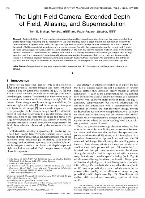
BISHOP AND FAVARO: THE LIGHT FIELD CAMERA: EXTENDED DEPTH OF FIELD, ALIASING, AND SUPERRESOLUTION 975l ¼ H s r;ð1Þwhere l and r are rearranged as column vectors. H s embedsboth the camera geometry (e.g., its internal structure, thenumber, size, and parameters of the optics) and the scenedisparity map s. In general, the only quantities directlyobservable are the LF image l and the camera geometry, andone has to recover both r and s. Due to the dimensionality ofthe problem, in this manuscript we consider a two-stepapproach where we first estimate the disparity map s andthen recover the radiance r given s. In both steps, weformulate inference as an energy minimization.For now, assume that the disparity map s is known.Then, one can employ (SR) by estimating r directly from theobservations. Due to the fact that the problem may beparticularly ill-posed depending on the extent of thecomplete system, proper regularization of the solutionthrough prior modeling of the image data is essential. Wecan then formulate the estimation of r in the Bayesianframework. Under the typical assumption of additiveGaussian observation noise w, the model becomesl ¼ H s r þ w, to which we can associate a conditionalprobability funtion (PDF), the likelihood pðlj r; H s :Þ.We then introduce priors on r. We use a recentlydeveloped prior [31], [32], which can locally recover texture,in addition to smooth and edge regions in the image. Bycombining the prior pðrÞ with the likelihood from the noisyimage formation model we can then solve the maximuma posteriori (MAP) problem:^r ¼ arg max pðlj r; H s ÞpðrÞ:ð2ÞrThe MAP problem requires evaluating H s , whichdepends on the unknown disparity map s. To obtain s weconsider extracting views (images from different viewpoints)from the LF so that our input data are suitable for amultiview geometry algorithm (see Section 6). The multiviewdepth estimation problem can then be formulated asinferring a disparity map s ¼ : fsðc k Þg by finding correspondencesbetween the views for each 2D location c k visible inthe scene. Let ^V q denote the sampled view from the 2Dviewing direction q and ^V q ðkÞ the color measured at a pixelk within ^V q . Then, as we will see, depth estimation can beposed as the minimization of the joint matching error (plusa suitable regularization term) between all combinations ofpairs of views:E data ðsÞ ¼Xð ^V q1 ðk þ sðc k Þq 1 Þ ^V q2 ðk þ sðc k Þq 2 ÞÞ;8q 1 ;q 2 ;kwhere is some robust norm and q 1 ;q 2 are the 2D offsetsbetween each view and the central view (the exactdefinition is given in Section 6.1). In practice, to savecomputational effort, only a subset of view pairs fq 1 ;q 2 gmay be used in (3). Notice that this definition of the 2Doffset implicitly fixes the central view as the reference framefor the disparity map s.As the views may be aliased, minimizing (3) is liable tocause incorrect depth estimates around areas of highspatialfrequency in the scene. Put simply, even whenscene objects are Lambertian and without the presence ofnoise, the views might not satisfy the photoconsistencyð3ÞFig. 4. (a) 2D Schematic of a LF camera. Rays from a point p are splitinto several beams by the microlens array. (b) Three example imagescorresponding to the colored planes in space (dashed) and theirconjugates (solid). Top: p 0 before microlenses; subimages flipped.Middle: p 0 on microlenses; no repetitions. Bottom: p 0 is virtual, beyondthe microlenses; no flipping.criterion sufficiently well so that E data may not have aminimum at the true depth map. Moreover, subpixelaccuracy is usually obtained through interpolation. Thismight be a reasonable approximation when the viewscollect samples of a band-limited (i.e., sufficiently smooth)texture. However, as shown in Fig. 3, this is not the casewith LF cameras. Therefore, we have to explicitly definehow samples are interpolated and study how this affectsthe matching of views.We shall also see that there are certain planes where thesample locations from different views coincide. At theseplanes, aliasing no longer affects depth estimation, but extrainformation for (SR) is diminished.4 IMAGE FORMATION OF A LIGHT-FIELD CAMERAIn this section, we derive the image formation model of aplenoptic camera, and define the relationship betweendifferent camera parameters. To yield a practical computationalmodel suitable for our algorithm (Section 7), weinvestigate the imaging process with tools from geometricoptics [33], ignoring diffraction effects, and using the thinlens model. We will also analyze sampling of the LF cameraby using the phase-space domain [7].4.1 Imaging ModelIn our investigation, we rebuilt a light field camera similarto that of Ng et al. [3]—essentially a regular camera with amicrolens array placed near the sensor (see Fig. 4)—but, asin [21], we consider the imaging system under a generalconfiguration of the optical elements. However, unlike inany previous work, we determine the image formationmodel of the camera so that it can be used for SR or moregeneral tasks.We use a general 3D scene representation (ignoringocclusions), consisting of the all-focused image, or radiance,rðuÞ (as captured by a pinhole camera, i.e., with aninfinitesimally small aperture), plus a depth map zðuÞassociated with each point u. Both r and z are defined at themicrolens array plane such that r is the all-focused imagethat would be captured by a regular camera. In this way, wecan analyze both the PSF of each point in space (correspondingto a column of H s ) and sampling and aliasingeffects in the captured LF with a less bulky notation. Wefirst consider the equivalence between using points in space

BISHOP AND FAVARO: THE LIGHT FIELD CAMERA: EXTENDED DEPTH OF FIELD, ALIASING, AND SUPERRESOLUTION 977Fig. 7. (a) Choice of aperture sizes for fully tiling subimages. (b) Imagingthe purple vector under different microlenses. A point u on the radiancehas a conjugate point indicated by the triangle at u 0 , which is imaged by amicrolens centered at an arbitrary center c, giving a projected point atangle . A second microlens positioned at u images the same point at thecentral view ¼ 0 on the line through O. The scaling of the purple vectorto the green vectors is .The coordinates ðq; kÞ will be used often in the next sectionsto parameterize the light field, which is originally capturedwith respect to the coordinates ½i m ;j m Š T ¼ q þ Qk. Theinverse mapping isiðq; kÞ ¼ mod mþ Q $ %!Qj m 2 ;Q 2 ; ½i m ;j m Š Tþ 1 : ð7ÞQ 24.1.5 Ray Space RepresentationIn Fig. 8, we show an alternate view of sampling, aliasing,and blurring effects in the plenoptic camera, via the (2D) rayspace representation of Levin et al. [7]. In our version, weuse the internal camera coordinates: u (spatial) and theprojection of onto the main lens (angular). A point in thisspace represents a ray through the corresponding positionson the main lens and microlens array, while a ray withconstant color corresponds to a particular conjugate point(e.g., the vertical red rays are points on the microlens array,conjugate to the main lens plane in focus in space; differentslopes represent other depths, with the same colors as theplanes in Fig. 4). Each gray parallelogram indicates the raysin the LF that a sensor pixel integrates; their shear anglecorresponds to the conjugate plane the microlenses arefocused on. A column of parallelograms is one subimage,and a row represents a view. Gaps between parallelogramsare due to pixel fill-factor vertically, and microlens apertureshorizontally. To achieve the highest sampling accuracyachievable, the gray parallelogram should be aligned alonga ray of constant intensity (so that pixel integration does notlead to a loss of information). rðuÞ is the slice of the raysalong the x-axis.5 SUPERRESOLUTION LIMITS AND ANALYSIS OFMODEL5.1 SuperresolutionSo far we have found relations between points in space andtheir projections on the sensor, assuming infinitesimalmicrolens apertures. However, in general the image of apoint p 0 on the sensor is a pattern called the system PSF,whose shape depends on the projection of the finite aperturesonto the sensor. We will see that these blur sizes, as well asthe number of times a point is imaged under differentmicrolenses, can affect the SR quality.Fig. 8. Ray space diagram [7], with internal camera coordinates.(a) Apertures on the microlenses correspond to parallelograms. Theyellow region corresponds to objects inside the camera, while the greenline marks the conjugate image at 1, i.e., the object at distance F fromthe camera. (b) Microlens blur with finite apertures (vertical scale here isvin rather than 0v ).We would like to superresolve at resolutions close tothat of the original sensor. While we may render theestimate of r at any resolution, the actual detail that will berecovered will depend on a combination of factors relatedto how ill posed the inversion is, and how good our systemcalibration and priors are. Previous SR studies [34], [35],[36] showed in general that the performance of SRalgorithms decreases as blur size increases; it alsodecreases when the ratio of upsampling factor to numberof observations remains constant, but the upsamplingfactor increases. While our imaging model is ratherdifferent from those mentioned for regular SR, the samegeneral principles apply. We also point out some importantdesign considerations based upon these limitations.5.1.1 Main Lens DefocusThe cone of rays passing through p 0 causes a blur on themicrolens array determined by the main lens aperture. Thisblur disc determines how many microlenses capture lightfrom p 0 . With the Lambertian assumption, p 0 casts the samelight on each microlens, and this results in multiple copiesof p 0 in the LF (see first and third image in Fig. 4).Approximating this blur by a Pillbox with radius B 0 (i.e.,the unit volume cylinder, hðuÞ ¼ 1Bfor kuk 2 2 2 B2 and 0otherwise), the main lens blur radius isB ¼ Dv01 12 z 0 v 0 :ð8ÞTo characterize the number of repetitions of the samepattern in the scene, we must count how many microlensesfall inside the main lens blur disc. Therefore, in eachdirection we have#repetitions ¼ 2B d ¼ Dv01 1d z 0 v 0 : ð9ÞThis ratio is also evident in the ray space (Fig. 8) byconsidering how many columns (subimages) the blue rayon the right covers. In our SR framework, this numberdetermines how many subimages can be used to superresolvethe LF.5.1.2 Microlens BlurA necessary condition to superresolve the LF is that theinput views are aliased so that they sample different

978 IEEE TRANSACTIONS ON PATTERN ANALYSIS AND MACHINE INTELLIGENCE, VOL. 34, NO. 5, MAY 2012 ¼ : z 0system and by generalizing the microlenses to virtual onesvv 0 v 0 z : ð12Þ centered in the continuous coordinates c, rather than0discrete positions c k .Notice the relation to Lumsdaine and Georgiev’s magnificationfactor [21]. Here, however, we refer everything to acommon reference frame in r in order to compare multipledepths. Note that the number of repetitions may also berewritten in terms of as#reps ¼ D v 0 z 0d z 0 ¼ v0v 0 z 0v 0 þ vz 0 v v 0 ¼ 1 QFig. 9. (a) and (b) Microlens blur radius b versus scene depth z (in logjj d ;scale), for several settings of the microlens-to-CCD spacing v. Theð13Þmicrolens focal length f is 0.35 mm (note that Ng et al. [3] sets v ¼ f). where we used (6). Thus, since Q dis constant, as theThe main lens plane in focus is at 700 mm. Our model can work with anynumber of repetitions increases, the size of subimagesuitable settings. (c) Magnification factor between the radiance at themicrolens plane and each subimage, under similar settings.features decreases.The above equation formalizes the constraint that, forinformation, i.e., they are not just shifted and interpolatedversions of the same image. We discuss aliasing further inSection 6, but here it suffices to note that increasingsubimage blur reduces complementary information in theLF available to perform SR. The blur of each microlens thateach depth, the amount of information from r remainsconstant, but is split across a different number of subimages.What does change, however, is the effective blur, orthe integration region in r of a sensor pixel, as it scales withthe magnification factor .is fully covered by the main lens PSF (some are not, seeSection 7.1.2) is also a pillbox due to the microlens aperture, 5.1.4 Coincidence of Samples and Undersamplingwith radius (see Fig. 5):In this section, we show that samples from differentb ¼ dvmicrolenses coincide in space on some fronto-parallel1 1 12 fv 0 z 0 v planes. On these planes the aliasing requirements are notsatisfied and the SR restoration performance will decrease.where f is the microlens focal length. In Fig. 8, theWe shall see this experimentally in Section 8.2.2. One suchmicrolens blur is the horizontal projection of a ray onto plane is when the conjugate image lies on the microlensthe subimage pixels it intersects. Restoration performance isoptimal at depths where b ! 0 (rays like the purple one inFig. 8, with the same slope as the pixel shear), obtained forplane. Another is shown in Fig. 6, where r 0 is positionedsuch that the blue, red and black rays intersect inside thecamera at this depth. In Fig. 8, this degeneracy correspondspoints p 0 at a distance z 0 ¼ v 0 vfv f, and it will degrade to a ray passing through exactly the same point in aaway from these depths. When a microlens is not fully parallelogram in different subimages.inside the main lens PSF, then its blur radius is smaller (seeSection 7). For simplicity, consider the blur radius b 0 whenboth microlens and main lens share the same optical axis(see the general case in Section 7):To have an exact replica of a sample of r 0 under twomicrolenses, it must simultaneously project on two discretepixel coordinates. Considering two microlenses separatedby Nd, with N 2 Z, then the coordinate 0 under the firstb 0 ¼ min2Bb microlens must correspond to a coordinate NdðuÞ ¼T,d ;b : ð11Þ where T 2 Z. Also, for the corresponding pixel to be fullyinside the subimage, T< QNotice that as z 0 ! v 0 2. By substituting the expression, although b !1, the radius b 0 for T, we see that such microlenses must satisfy N

BISHOP AND FAVARO: THE LIGHT FIELD CAMERA: EXTENDED DEPTH OF FIELD, ALIASING, AND SUPERRESOLUTION 979Let us use Fig. 7b to consider: 1) how a vector or a pointis mapped from the radiance onto the sensor under anarbitrary microlens at c, and 2) where the correspondencesof the point c lie in other views if this point is at angle inone view.To find 1, begin with the purple vector u c. By similartriangles and by projecting first through O to the red vectorand then through c to the green one, we see that the purplevector image under lens c is scaled by (see (12)). Notingthat the local origin is 0 , we can equivalently express themapping of the point u in r (the tip of the vector) through alens at c to a subimage correspondence at ¼v 0v z 0 ðuÞz 0 ðuÞ v 0 ðc uÞ ð15Þ¼ ðuÞðc uÞ: ð16ÞBy inverting this relation, the original point u in rcorresponding to any and c is uð; cÞ ¼cðuÞ, and theviews and subimages are related to the radiance as:V ðcÞ ¼S c ðÞ ¼rðcðuÞ Þ. V ðcÞ and S c ðÞ differ only bywhich of or c we hold fixed.Considering (2), we can reformulate the above ideas. Fora point c 1 in a particular view at angle 1 , we can find itscorrespondence uð 1 ;c 1 Þ in the radiance, and then solve forc 2 so that V 1 ðc 1 Þ¼rðuÞ ¼V 2 ðc 2 Þ, for arbitrary 2 . Thetrick is to refer everything to a common reference framewhere ðuÞ is defined (the points share the same depth/magnification). We choose this reference frame to be thecentral view 0 ¼ 0, where we have c ¼ u and V 0 ðcÞ ¼V 0 ðuÞ ¼rðuÞ, i.e., this view samples the radiance directly.This can be seen in Fig. 7b as the microlens placed at u.The result is that c 1 ¼ u þ 1ðuÞand c 2 ¼ u þ 2ðuÞ . Thediscrete version of these equations, which we describebelow, leads us to the view matching in (3). We may alsointerpret these matches as positions ðc 1 ; 1 Þ and ðc 2 ; 2 Þ onthe same ray in Fig. 8, where 1 is the slope of the ray and uis where the ray intersects the x-axis.6.2 Discretization of Views and SubimagesV ðcÞ and S c ðÞ are defined for all possible c and . Inpractice, if we approximate the microlens array with anarray of pinholes, 4 only a discrete set of samples in eachview is available, corresponding to the pinholes at positionsc ¼ c k . Furthermore, the pixels in each subimage sample thepossible views at q . Therefore, we define the discreteobserved view ^V q at angle q as the image^V q ðkÞ ¼ : V ðc q kÞ¼r c k qðc k Þ¼ rdk ð sðc k ÞdqÞ; ð17Þwhere we defined the view disparity, in pixels per view, assðuÞ ¼ : 1d ðuÞ :ð18ÞThe discrete disparity is sðc k Þ and depends on the depth z.The discretized subimages are just a rearrangement of the4. We will see that the addition of microlens blur due to finite apertureswill integrate around these sample locations.LF samples; in fact they are also defined by (17), i.e.,^S k ðqÞ ¼ ^V q ðkÞ.In a similar manner to the continuous case, two discreteviews at q 1 and q 2 can be related via the reference view as^V q1 ðk þ sðc k Þq 1 Þ¼ ^V 0 ðkÞ ¼ ^V q2 ðk þ sðc k Þq 2 Þ;ð19Þthus obtaining the matching terms in (3). By defining thesubimage disparity, tðc k Þ¼ : 1sðc kÞ, subimages may also berelated via^S k0 þk 1ðq þ tðc k0 Þk 1 Þ¼ ^S k0 ðqÞ ¼ ^S k0 þk 2ðq þ tðc k0 Þk 2 Þ:ð20ÞThe discrete views in (17) are just samples of r withspacing d, but different shifts sðuÞdq, depending on theview angle and depth. The multiview disparity estimationtask is to estimate sðuÞ by shifting the views so that they arebest aligned. However, this requires subpixel accuracy, i.e.,an implicit or explicit reconstruction of r in the continuum.According to the sampling theorem, r may be reconstructedexactly from the samples taken at spacing d so long as theoriginal radiance image contains no frequencies higher thanthe Nyquist rate f 0 ¼ 12d. In practice, this condition is oftennot satisfied due to the low resolution of the views, andaliasing occurs. Observe that a larger microlens pitch leadsto greater aliasing of the views.6.3 Ideal and Approximate Antialiasing FilteringIdeally the LF should be antialiased before views areextracted, i.e., we should combine information acrossviews. We make use of an extension of the samplingtheorem by Papoulis [37], showing that if r is bandlimitedwith a bandwidth f r ¼ Qf 0 =, then it can be accuratelyreconstructed on a grid with spacing if we have Q=sets of samples available, with any shifts or linear filteringof the original signal. This implies that we obtain thecorrectly antialiased views ~V q ðkÞ from the sampled lightfield as follows:1. Use a reconstruction method FðÞ jointly on allsamples to obtainrðuÞ ¼Fðf^V q 0ðk0 Þg;uÞ ¼ X k 0 ;q 0k 0 ;q 0ðuÞ ^V q 0ðk0 Þfor some set of interpolating kernels k 0 ;q (we could0use the theorem from [37] to define these kernels,but essentially this operation corresponds to applyingany (SR) method).2. Filter these samples with an antialiasing filter h f0 atthe correct Nyquist rate f 0 to obtain~rðuÞ ¼ðh f0 ?rÞðuÞ:3. Resample to obtain ~V q ðkÞ ¼~rðc k þ sðuÞ d qÞ.A drawback of this approach is that a computationallydemanding (SR), as well as filtering at a high resolutionbefore extracting low resolution views, is required. Moreover,a chicken-and-egg type problem is apparent: Thedepth-dependent filters depend on the unknown depthmap. Thus, we look at an approximate but efficient method.Rather than filtering the whole LF simultaneously, wefilter each subimage directly, bypassing the reconstruction

980 IEEE TRANSACTIONS ON PATTERN ANALYSIS AND MACHINE INTELLIGENCE, VOL. 34, NO. 5, MAY 2012Fig. 10. Antialiasing filtering, increasing from (a) to (d). Top row: Detail ofsubimages. Middle: Corresponding filtered full view. Bottom: Magnifieddetail of the view.step. Since each subimage is a windowed projection of r ontothe sensor (ignoring blur for now), we may equivalentlyproject the filters in the same way. This is approximate atsubimage boundaries, where we must use filters with asupport limited to the domain of . Hence, we upper boundthe filter size using a Lanczos windowed version of the idealSinc kernel. The antialiasing filter h f0 , defined in r, isprojected onto the sensor via the conjugate image at z 0 , i.e.,scaling by jj, as in (16). Hence, the scaled filter has physicalcutoff frequency f 0 jj. We propose an iterative method,beginning with a strong antialiasing filter, and refining theestimate based upon the current depth map. Too muchfiltering might remove detail for valid matches, while toolittle may leave aliasing behind (see Fig. 10). We summarizethe algorithm as follows:1. Initialize all filters with cutoff f 0 jj max , i.e., assumingthe depth which yields the most aliasing in theworking volume.2. Estimate the disparity map sðc k Þ (see Section 6.5).3. Rearrange the views as subimages ^S k ðqÞ.4. For each k, filter ^S k ðqÞ by h f0 jj, using ¼ dsðc k Þ .5. Repeat from 2 until the disparity map update isnegligible.6.4 Microlens BlurWith finite microlens apertures each pixel integrates over alarger area and aliasing is reduced due to additional blur(see Fig. 8). By taking this into account we can use milderantialiasing.As the antialiasing filter for an array of pinhole lenses isa Sinc filter, we define the antialiasing kernel size as this1filter’s first zero crossing, i.e.,2f 0 jj. The correct amount ofantialiasing is readily obtained by comparing this size withthe blur radius b. Then, the final antialiasing filter has a1radius approximated as j2f 0 jjbj, clipped from below at 0and from above by d 2. Fig. 11 shows the resulting filtersizes for the settings used in Section 8.1.2.6.5 Regularized Depth EstimationWe now have all the necessary ingredients to work on theenergy introduced in (3). The depth map s is discretized atc k as a vector s ¼fsðuÞg u2fck ;8kg. Due to the ill-posednessof the problem, we introduce regularization, favoringpiecewise constant solutions by using the total variationFig. 11. Microlens blur and antialiasing filter sizes versus depth.(a) Overlap of filter kernel size and microlens blur radius for differentdisparity (depth) values. (b) Resulting antialiasing kernel size fordifferent depth values.term krsðuÞk 1 , where r is the 2D gradient with respect tou. Hence, we wish to solve~s ¼ arg min E data ðsÞþkrsðuÞks1 ; ð21Þwhere >0 determines the tradeoff between regularizationand data fidelity (in our experiments we chose ¼ 10 3 ).We minimize this energy by using an iterative solution. Bynoticing that E data can be written as a sum of termsdepending on a single entry of s at once, we find aninitialization s 0 by performing a fast brute force search inE data for each c k independently. Then, we approximateE data via a second order Taylor expansion, i.e.,E data ðs tþ1 Þ’E data ðs t ÞþrE data ðs t Þðs tþ1s t Þþ 1 2 ðs tþ1 s t Þ T H Edata ðs t Þðs tþ1 s t Þ;ð22Þwhere rE data and H Edata are the gradient and Hessian ofE data , and subscripts t and t þ 1 denote iteration number.To ensure our local approximation is convex we take theabsolute value (component wise) of H Edata ðs t Þ. In the caseof the term krsðuÞk 1 , we use a first order Taylor expansionof its gradient. Computing the Euler-Lagrange equations ofthe approximate energy E with respect to s tþ1 thislinearization results inrE data ðs t ÞþjH Edata ðs t Þjðs tþ1 s t Þ r rðs tþ1 s t Þ¼ 0;jrs t jð23Þwhich is a linear system in the unknown s tþ1 , and can beefficiently solved using conjugate gradients (CG).7 LIGHT FIELD SUPERRESOLUTIONSo far we devised an algorithm to reduce aliasing in viewsand estimate the depth map. We now define a computationalPSF model, and formulate the MAP problempresented in Section 3.7.1 Light Field Camera Point Spread Function7.1.1 PSF DefinitionCombining the analysis from Sections 4 and 5, we candetermine the system PSF of the plenoptic camera h LIs —which is unique for each point in 3D space, and will be acombination of main lens and microlens array blurs. Wedefine this PSF such that the intensity at a pixel i caused bya unit radiance point at u with a disparity sðuÞ is

BISHOP AND FAVARO: THE LIGHT FIELD CAMERA: EXTENDED DEPTH OF FIELD, ALIASING, AND SUPERRESOLUTION 981h LIsði; uÞ ¼hMLkðiÞ ð qðiÞ;uÞh LkðiÞ ð qðiÞ;uÞ; ð24Þwhere kðiÞ and qðiÞ are given by (7). In a Lambertian scene,the image l captured by the light field camera is thenZlðiÞ ¼ h LIs ði; uÞrðuÞdu: ð25ÞWe define the microlens point spread function h LkðiÞconsidering the main lens diameter to be infinite. This gives8< 1h LkðiÞ ð qðiÞ;uÞ ¼ b 2 qðiÞ ðuÞðc kðiÞ uÞ ðuÞ2 z0 fz 0 fand negative otherwise.7.1.2 Main Lens VignettingAs seen in Fig. 4 a microlens may only be partially hit by themain lens blur disc, which results in clipped microlens PSF;this effect is modeled by the product of h LkðiÞand hMLkðiÞ . Alsonotice that depending on the camera settings and thedistance of the object from the camera, the PSF under eachmicrolens may be flipped.7.1.3 DiscretizationTo arrive at a computational model, we discretize thespatial coordinates as u n with n 2f1...Ng and use thepixel coordinates ½i m ;j m Š T with m 2f1...Mg. Then, (25)can be rewritten in matrix-vector form l ¼ H s r as in (1).rðnÞ ¼ : rðu n Þ and lðmÞ ¼ : lði m ;j m Þ are the discrete vectorizedversions of l and r. H s 2 IR MN is the sparse matrixH s ðm; nÞ ¼ : h LIsðu n Þ ði m ;u n Þ;ð28Þwhere each column is the PSF corresponding to theupsampled depth map at that point (i.e., it is a nonstationaryoperator). Also, we are free to choose the spacing ofthe samples u n as ; setting ¼ 1 recovers the sameresolution as the original sensor; however, depending onthe camera settings, too high a resolution will not revealadditional detail. Hence, we choose based on our analysisof the limits of the LF camera as described in the previoussections. Note that, in particular, if the microlens diameteris reduced, more image detail will be visible (although lesslight efficient). Typically, we use ¼ 2 to reduce computationalload. The upsampling factor compared to the originalviews is Q=.7.2 Bayesian SuperresolutionWe use the Bayesian framework to estimate r, where allunknowns are treated as stochastic quantities. Withadditive Gaussian observation noise w Nð0; 2 wIÞ, themodel becomes l ¼ H s r þ w, and the probability ofobserving a given light field l in (1) may be written aspðlr; H s ; 2 w ;sÞ¼Nðl H s ;r; 2 w I Þ.We then introduce priors on the unknowns (assuming sis already estimated). Many recent image restoration worksmake use of nonstationary edge preserving priors. Forexample, total variation or modeling heavy-tailed distributionsof image gradients or wavelet subbands are popular[38]. We apply a recently developed Markov random field(MRF) prior [31], [32] which extends such ideas tomodeling higher order neighborhoods. It uses a localautoregressive (AR) model, whose parameters are alsoinferred, and leads to a conditionally Gaussian priorpðrj a; v :Þ¼Nðrj 0; C 1 Q v C T :Þ, where matrix C applieslocally adaptive regularization using AR parameters a; Q vis a diagonal matrix of local variances v . We estimate theseparameters using conjugate priors, which lets us setconfidences on their likely values. The resulting Gaussian—inverse-gammacombination also represents inferencewith a heavy-tailed Student-t, considering the marginaldistribution, corresponding to sparsity in the texture model.The SR inference procedure therefore involves finding anestimate of the parameters r; a; v ; 2 wgiven the observations land an estimate of H s . Direct maximization of the posteriorpðr; a; v ; w j l; H s Þ/pðljH s Þpðrj a; v Þpða; v ; 2 wÞ is intractable;hence, we use variational Bayes estimation withthe mean field approximation to obtain an estimate of theparameters.7.3 Numerical ImplementationThe variational Bayesian procedure requires alternateupdating of approximate distributions of each of theunknown variables. The approximate distribution for r isa Gaussian withIE½rŠ ¼cov½rŠ 2w HT s l;ð29Þcov½rŠ 1 ¼ C T Q 1v C þ w 2 HT s H s : ð30ÞThis update of IE½rŠ can be found solving M T Mr ¼ M T y,with Q 1v¼ L T L, M ¼½w 1HTs jCT LŠ T , and y ¼½w 1lTj0Š T .However, due to the large size of this linear system, we solveefficiently using CG for each step. Each CG iteration requiresmultiplying by H s and its transpose once, which weimplement as a sparse matrix formed using a look-up tableof precomputed PSFs from each point in 3D space. Theimage restoration procedure is run in parallel tasks acrossrestored tiles of size up to around 400 400 pixels, whichare trimmed to the valid region and then seamlesslymosaiced (size is limited such that the nonstationary H scan be preloaded into memory). We run experiments inMATLAB on an 8-core Intel Xeon processor with 2 GB ofmemory per task. Precalculating the look-up table can takeup to 10 minutes per depth plane (depending on PSF size);however, restoration is faster: Each CG iteration takesaround 0.1-0.5 seconds (again depending on depth). Goodconvergence is achieved after typically 100 to 150 iterations.The AR model parameters are recomputed every few CGiterations, taking around 1-2 seconds. Notice that since themodel is linear in the unknown r, convergence is guaranteed

982 IEEE TRANSACTIONS ON PATTERN ANALYSIS AND MACHINE INTELLIGENCE, VOL. 34, NO. 5, MAY 2012TABLE 1Average L 2 Norm Disparity Error (Pixels per View 10 3 ),against Noise Levels, Filtering Method: No (A), Ideal (B),and Iterative Filtering (C), 4 textures and at 2 scales:Fine (1), Coarse (2)Fig. 12. Synthetic data: antialiasing filtering. Top: LF image of a sum-oftwo-sinusoidstexture (at five depth planes). Bottom: (a) One extractedview, containing aliasing. (b) The view filtered with the estimated depth(left) and the corresponding high-frequency image (right). (c) As in (b),but using the true depth; there is little difference between the two.(d)-(f) Enlarged portions of the last depth step in (a)-(c).by the convexity of the cost functional. The total runtime pertile is typically 30-60 seconds, depending on depth.8 EXPERIMENTSThe antialiased 3D depth estimation method is tested on bothsynthetic and real data in Section 8.1. Then, the proposed SRmethod is tested similarly in Section 8.2. We also evaluaterestoration performance in Section 8.2.2, comparing to othercomputational and regular camera systems.8.1 Antialiased Depth Estimation8.1.1 Synthetic DataThe scene in Fig. 12 consists of five steps at different depths,with a texture that is the sum of sinusoids at 0.2 and 1.2 timesthe views’ Nyquist rate f 0 , therefore the higher frequency isaliased in the views (but not in the subimages). The scene hasdisparities in the range s ¼ 0:24 to 0.44 pixels per view. Wesimulate a camera with Q ¼ 15, ¼ 9:05 10 6 m, d ¼0:135 mm, v ¼ 0:5 mm, f ¼ 0:5 mm, v 0 ¼ 91:5 mm, andF ¼ 80 mm. Note that for these settings, the microlens bluris small but nonnegligible, varying between 1.2 and 2.1 pixelsradius. We use the 9 9 pixel central region of each subimagefor depth estimation. Fig. 12 shows one of the 81 extractedviews, and the result of filtering with the estimated and truedisparity maps, with the aliased component separated out. InFig. 13, we compare the resulting disparity maps recoveredwith no antialiasing filtering, the iterative method, with thecorrect antialiasing filter (the errors at depth transitions occurdue to lack of occlusion modeling in the synthesized data),and the ground truth.We also test the algorithm’s performance, repeating theexperiment at 16 depths (for s ¼ 0:1 to 0.6). Results in Table 1show the average L 2 norm per pixel of the error between theRow header is in the format (Texture/Scale).ground truth and the disparity maps obtained with differentfiltering. We use the sinusoidal pattern and three texturestaken from the Brodatz data set (http://sipi.usc.edu/database/database.cgi?volume=textures). Each texture isresized to 380 380 pixels, and tested again with the central50 percent enlarged to this size to give a coarser scale. Wetest both the noise-free case and with additive Gaussianobservation noise at two different levels. The texturescontain different proportions of high and low frequencies;when more high frequencies are removed due to aliasing,matching performance decreases as less texture contentremains to match.8.1.2 Real DataThe use of small f=10 microlens apertures and a largemicrolens spacing (27 pixels per subimage) results insignificant aliasing in the data from Georgiev andLumsdaine [22] (kindly made available by Georgiev athttp://www.tgeorgiev.net), hence it is a good test for theantialiasing algorithm. Other camera settings are asdescribed in [6], [22]. Subimages and view details of thisdata are shown in Fig. 10, for different filters, toappreciate the effect of an incorrect size. In Fig. 14, weshow the disparity maps obtained at different steps of theiterative algorithm (the first iteration is essentially astandard multiview stereo result), along with the finalregularised result. Notice that there is a progressivereduction in the number of artifacts and that the disparitymap becomes more and more accurate. The estimatedFig. 13. Depth estimates. From top to bottom: Results obtained withoutfiltering, with the iterative method, with the correct filtering, and theground truth. Each row shows the disparity map (a) without and (b) withregularization. Notice how the results obtained with the estimated depthare extremely similar to those obtained with the correct filter.Fig. 14. Depth estimates on real data. (a) Disparity map estimateobtained without regularization (left) and for increasing filtering iterations(middle and right). (b) L 1 regularized disparity map, from the energy ofthe third iteration. (c) Regularized depth map for the puppets data set(Fig. 18).

BISHOP AND FAVARO: THE LIGHT FIELD CAMERA: EXTENDED DEPTH OF FIELD, ALIASING, AND SUPERRESOLUTION 983Fig. 15. Synthetic results. (a) Top: True radiance. (b) Top: True depthmap. (c) Top: Light field image simulated with our model. (a) Bottom: LFimage rearranged as views. (b) Bottom: Central view (as in a traditionalrendering [3]). (c) Bottom: (SR) radiance restored with our method.disparities lie in the range s ¼ 0:34 to 0.31, with themiddle book being around the main lens plane-in-focus(zero disparity). Regularized depth maps from other realdata sets are also shown in Figs. 14 and 1.8.2 Superresolution Results8.2.1 Synthetic DataIn Fig. 15, we simulate LF camera data using (1) and asynthetic depth map, then apply the SR algorithm (usingthe known depth) to recover a high resolution focussedimage. The simulated scene lies in the range 800-1,000 mm,each of the 49 views (i.e., we use only the 7 7 pixelcentral portion of each subimage in this experiment) is a19 29 pixel image. The magnification gain is about seventimes along each axis.8.2.2 LF Camera/SR Performance TestingFirst, we test how the proposed SR method compares tolow-resolution integral refocusing [3] and the method ofLumsdaine and Georgiev [6]. We generate synthetic LF datausing our model and the same settings as Section 8.1.1, withthe “Bark” texture from the Brodatz database positioned ona sequence of 110 planes with depths in the range 486-1,074mm. We omit planes near the main lens plane-in-focuswhere

984 IEEE TRANSACTIONS ON PATTERN ANALYSIS AND MACHINE INTELLIGENCE, VOL. 34, NO. 5, MAY 2012Fig. 16. L2 error results comparison. (a) Restoration performance versus depth of our method and the method of [6] on the simulated LF camerausing our camera settings and the Brodatz “Bark” texture, with input intensity range 0-1. The (ISNR) is compared for several different levels ofobservation noise (standard deviation w ). Solid lines show our restoration method, dashed using the method of Lumsdaine and Georgiev [6] on thesame data. We have not restored depths where

BISHOP AND FAVARO: THE LIGHT FIELD CAMERA: EXTENDED DEPTH OF FIELD, ALIASING, AND SUPERRESOLUTION 985Fig. 18. Superresolution on real data Top row: Data from Georgiev and Lumsdaine [22] ( ¼ 1:4); Bottom row: “puppets” data set ( ¼ 3). (a) Nearestneighbourinterpolation of one view. (b) High-resolution view using method of Lumsdaine and Georgiev [6]. (c) View superresolved with our method.enabling full 3D repositioning and rotation without removingthe back. After manual correction, any residual error inthe captured images is removed by automatic homographybasedrectification (consistent to 1 20pixel across the sensor),and photometric calibration.After calibration, we estimate the depth map (see Fig. 14),and use its upsampled version to construct H s . We comparewith the restoration produced by the method in [6],modified to scale the subimages locally depending on thedepth map. Clearly, we obtain sharper results with our data,due to deconvolution (although there are a few errorsparticularly around depth transitions, that may be due todepth map errors and lack of occlusion modeling). With thedata in [22], there is less improvement from deconvolutionsince the microlens apertures (which sacrifice light and,hence, SNR) reduce the blur size, but the use of anintegrated restoration model also suppresses artifacts, forexample, the lines at the bottom of the image and in thebackground. The results in Fig. 18 consist of 6 5 tiles of125 125 pixels in the left column and 16 19 tiles of 135 135 pixels in the right column.We reiterate that our methods are general enough towork with any camera settings, though certain settings maysuit better certain tasks. One important tradeoff is in thechoice of the microlens aperture as done in [22]. Smallmicrolens apertures require more light, but also allow therecoverery of an all-focused image at about the detectorsresolution. On the other hand, large microlens apertures aremore light efficient, but result in an effective recoveredimage with lower resolution.9 CONCLUSIONSWe have presented a formal methodology for the restorationof high-resolution images from light field datacaptured from a LF camera, which is normally limited toreturning images at the lower resolution of the number ofmicrolenses in the camera. In our methodology, the 3Ddepth of the scene is first recovered by matchingantialiased light field views, and then deconvolution isperformed. This procedure makes the LF camera moreuseful for traditional photography applications; we havealso shown the performance benefit of the LF camera forextended depth of field over other camera designs. In thefuture, we hope to use simultaneous depth estimation andsuperresolution, as well as extending the model to non-Lambertian and occluded scenes.ACKNOWLEDGEMENTSThe authors wish to thank Mohammad Taghizadeh and thediffractive optics group at Heriot-Watt University forproviding them with the microlens arrays and for stimulatingdiscussions, and Mark Stewart for designing andbuilding their microlens array interface. This work hasbeen supported by EPSRC grant EP/F023073/1(P).

986 IEEE TRANSACTIONS ON PATTERN ANALYSIS AND MACHINE INTELLIGENCE, VOL. 34, NO. 5, MAY 2012REFERENCES[1] E.H. Adelson and J.Y. Wang, “Single Lens Stereo with aPlenoptic Camera,” IEEE Trans. Pattern Analysis and MachineIntelligence, vol. 14, no. 2, pp. 99-106, Feb. 1992.[2] T. Georgeiv and C. Intwala, “Light Field Camera Design forIntegral View Photography,” technical report, Adobe Systems,2006.[3] R. Ng, M. Levoy, M. Brédif, G. Duval, M. Horowitz, and P.Hanrahan, “Light Field Photography with a Hand-Held PlenopticCamera,” Technical Report CSTR 2005-02, Stanford Univ., Apr.2005.[4] A. Veeraraghavan, R. Raskar, A.K. Agrawal, A. Mohan, and J.Tumblin, “Dappled Photography: Mask Enhanced Cameras forHeterodyned Light Fields and Coded Aperture Refocusing,” ACMTrans. Graphics, vol. 26, no. 3, p. 69, 2007.[5] M. Levoy, R. Ng, A. Adams, M. Footer, and M. Horowitz, “LightField Microscopy,” ACM Trans. Graphics, vol. 25, no. 3, pp. 924-934, 2006.[6] A. Lumsdaine and T. Georgiev, “The Focused Plenoptic Camera,”Proc. IEEE Int’l Conf. Computational Photography, Apr. 2009.[7] A. Levin, W.T. Freeman, and F. Durand, “Understanding CameraTrade-Offs through a Bayesian Analysis of Light Field Projections,”Proc. European Conf. Computer Vision, pp. 619-624, 2008.[8] G. Lippmann, “Epreuves Reversibles Donnant la Sensation duRelief,” J. Physics, vol. 7, no. 4, pp. 821-825, 1908.[9] K. Fife, A. El Gamal, and H.-S. Wong, “A 3D Multi-ApertureImage Sensor Architecture,” Proc. IEEE Custom Integrated CircuitsConf., pp. 281-284, 2006.[10] C.-K. Liang, G. Liu, and H.H. Chen, “Light Field AcquisitionUsing Programmable Aperture Camera,” Proc. IEEE Int’l Conf.Image Processing, pp. V233-236, 2007.[11] M. Ben-Ezra, A. Zomet, and S. Nayar, “Jitter Camera: HighResolution Video from a Low Resolution Detector,” Proc. IEEE CSConf. Computer Vision and Pattern Recognition, vol. 2, 2004.[12] W. Cathey and E. Dowski, “New Paradigm for Imaging Systems,”Applied Optics, vol. 41, no. 29, pp. 6080-6092, 2002.[13] H. Nagahara, S. Kuthirummal, C. Zhou, and S.K. Nayar, “FlexibleDepth of Field Photography,” Proc. 10th European Conf. ComputerVision, Oct. 2008.[14] S.C. Park, M.K. Park, and M.G. Kang, “Super-Resolution ImageReconstruction: A Technical Overview,” IEEE Signal ProcessingMagazine, vol. 20, no. 3, pp. 21-36, May 2003.[15] A. Katsaggelos, R. Molina, and J. Mateos, Super Resolution of Imagesand Video. Morgan & Claypool, 2007.[16] S. Borman and R. Stevenson, “Super-Resolution from ImageSequences—A Review,” Proc. Midwest Symp. Circuits and Systems,pp. 374-378, 1999.[17] M.K. Ng and A.C. Yau, “Super-Resolution Image Restoration fromBlurred Low-Resolution Images,” J. Math. Imaging and Vision,vol. 23, pp. 367-378, 2005.[18] S. Farsiu, D. Robinson, M. Elad, and P. Milanfar, “Advances andChallenges in Super-Resolution,” Int’l J. Imaging Systems andTechnology, vol. 14, pp. 47-57, 2004.[19] B.R. Hunt, “Super-Resolution of Images: Algorithms, Principles,Performance,” Int’l J. Imaging Systems and Technology, vol. 6, no. 4,pp. 297-304, 2005.[20] W.-S. Chan, E. Lam, M. Ng, and G. Mak, “Super-ResolutionReconstruction in a Computational Compound-Eye ImagingSystems,” Multidimensional Systems and Signal Processing, vol. 18,no. 2, pp. 83-101, Sept. 2007.[21] A. Lumsdaine and T. Georgiev, “Full Resolution LightfieldRendering,” technical report, Indiana Univ. and Adobe Systems,2008.[22] T. Georgiev and A. Lumsdaine, “Depth of Field in PlenopticCameras,” Proc. Eurographics 2009, 2009.[23] M. Levoy and P. Hanrahan, “Light Field Rendering,” Proc. ACMSiggraph, pp. 31-42, 1996.[24] J. Stewart, J. Yu, S.J. Gortler, and L. McMillan, “A NewReconstruction Filter for Undersampled Light Fields,” Proc. 14thEurographics Workshop Rendering, pp. 150-156, 2003.[25] J.-X. Chai, S.-C. Chan, H.-Y. Shum, and X. Tong, “PlenopticSampling,” Proc. ACM Siggraph, pp. 307-318, 2000.[26] A. Isaksen, L. McMillan, and S.J. Gortler, “Dynamically ReparameterizedLight Fields,” Proc. ACM Siggraph, pp. 297-306, 2000.[27] R. Ng, “Fourier Slice Photography,” Proc. ACM Siggraph, vol. 24,no. 3, pp. 735-744, 2005.[28] V. Vaish, M. Levoy, R. Szeliski, C. Zitnick, and S.B. Kang,“Reconstructing Occluded Surfaces Using Synthetic Apertures:Stereo, Focus and Robust Measures,” Proc. 26th IEEE CS Conf.Computer Vision and Pattern Recognition, vol. 2, pp. 2331-2338, 2006.[29] T.E. Bishop, S. Zanetti, and P. Favaro, “Light Field Superresolution,”Proc. IEEE Int’l Conf. Computational Photograph, Apr.2009.[30] T.E. Bishop and P. Favaro, “Plenoptic Depth Estimation fromMultiple Aliased Views,” Proc. 12th IEEE Int’l Conf. Conf. ComputerVision Workshops, 2009.[31] T.E. Bishop, R. Molina, and J.R. Hopgood, “Blind Restoration ofBlurred Photographs via AR Modelling and MCMC,” Proc. IEEE15th Int’l Conf. Image Processing, 2008.[32] T.E. Bishop, “Blind Image Deconvolution: Nonstationary BayesianApproaches to Restoring Blurred Photos,” PhD dissertation, Univ.of Edinburgh, 2008.[33] M. Born and E. Wolf, Principles of Optics. Pergamon, 1986.[34] Z. Wang and F. Qi, “Analysis of Multiframe Super-ResolutionReconstruction for Image Anti-Aliasing and Deblurring,” Imageand Vision Computing, vol. 23, no. 4, pp. 393-404, Apr. 2005.[35] D. Robinson and P. Milanfar, “Fundamental Performance Limitsin Image Registration,” IEEE Trans. Image Processing, vol. 13, no. 9,pp. 1185-1199, Sept. 2004.[36] S. Baker and T. Kanade, “Limits on Super-Resolution and How toBreak Them,” IEEE Trans. Pattern Analysis and Machine Intelligence,vol. 24, no. 9, pp. 1167-1183, Sept, 2002.[37] A. Papoulis, “Generalized Sampling Expansion,” IEEE Trans.Circuits and Systems, vol. 24, no. 11, pp. 652-654, Nov. 1977.[38] E.P. Simoncelli, “Statistical Modeling of Photographic Images,”Handbook of Image and Video Processing, A. Bovik, ed., second ed.,Academic Press, Jan. 2005.[39] C. Zhou and S. Nayar, “What Are Good Apertures for DefocusDeblurring?” Proc. IEEE Int’l Conf. Computational Photography,2009.Tom E. Bishop received the MEng degree inelectronic and information engineering from theUniversity of Cambridge (Pembroke College) in2004, and the PhD degree in engineering fromthe University of Edinburgh in 2009. From 2008until 2011, he was a postdoctoral researcher atHeriot Watt University. Since March 2011, hehas worked as a researcher at AnthropicsTechnology Ltd., London. His research interestsinclude computational photography, inverseproblems, image modeling, and blind deconvolution. He is amember of the IEEE.Paolo Favaro received the DIng degree fromthe Università di Padova, Italy in 1999, and theMSc and PhD degrees in electrical engineeringfrom Washington University, St. Louis, Missouri,in 2002 and 2003, respectively. He was apostdoctoral researcher in the ComputerScience Department of the University of California,Los Angeles and subsequently at theUniversity of Cambridge, United Kingdom. Heis now assistant professor in the Joint ResearchInstitute for Signal and Image Processing between the University ofEdinburgh and Heriot-Watt University, United Kingdom. His researchinterests are in computer vision, computational photography, inverseproblems, convex optimization methods, and variational techniques. Heis a member of the IEEE.. For more information on this or any other computing topic,please visit our Digital Library at www.computer.org/publications/dlib.