The Light Field Camera: Extended Depth of Field, Aliasing, and ...

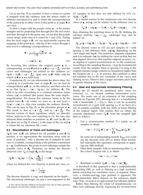
BISHOP AND FAVARO: THE LIGHT FIELD CAMERA: EXTENDED DEPTH OF FIELD, ALIASING, AND SUPERRESOLUTION 979Let us use Fig. 7b to consider: 1) how a vector or a pointis mapped from the radiance onto the sensor under anarbitrary microlens at c, and 2) where the correspondencesof the point c lie in other views if this point is at angle inone view.To find 1, begin with the purple vector u c. By similartriangles and by projecting first through O to the red vectorand then through c to the green one, we see that the purplevector image under lens c is scaled by (see (12)). Notingthat the local origin is 0 , we can equivalently express themapping of the point u in r (the tip of the vector) through alens at c to a subimage correspondence at ¼v 0v z 0 ðuÞz 0 ðuÞ v 0 ðc uÞ ð15Þ¼ ðuÞðc uÞ: ð16ÞBy inverting this relation, the original point u in rcorresponding to any and c is uð; cÞ ¼cðuÞ, and theviews and subimages are related to the radiance as:V ðcÞ ¼S c ðÞ ¼rðcðuÞ Þ. V ðcÞ and S c ðÞ differ only bywhich of or c we hold fixed.Considering (2), we can reformulate the above ideas. Fora point c 1 in a particular view at angle 1 , we can find itscorrespondence uð 1 ;c 1 Þ in the radiance, and then solve forc 2 so that V 1 ðc 1 Þ¼rðuÞ ¼V 2 ðc 2 Þ, for arbitrary 2 . Thetrick is to refer everything to a common reference framewhere ðuÞ is defined (the points share the same depth/magnification). We choose this reference frame to be thecentral view 0 ¼ 0, where we have c ¼ u and V 0 ðcÞ ¼V 0 ðuÞ ¼rðuÞ, i.e., this view samples the radiance directly.This can be seen in Fig. 7b as the microlens placed at u.The result is that c 1 ¼ u þ 1ðuÞand c 2 ¼ u þ 2ðuÞ . Thediscrete version of these equations, which we describebelow, leads us to the view matching in (3). We may alsointerpret these matches as positions ðc 1 ; 1 Þ and ðc 2 ; 2 Þ onthe same ray in Fig. 8, where 1 is the slope of the ray and uis where the ray intersects the x-axis.6.2 Discretization of Views and SubimagesV ðcÞ and S c ðÞ are defined for all possible c and . Inpractice, if we approximate the microlens array with anarray of pinholes, 4 only a discrete set of samples in eachview is available, corresponding to the pinholes at positionsc ¼ c k . Furthermore, the pixels in each subimage sample thepossible views at q . Therefore, we define the discreteobserved view ^V q at angle q as the image^V q ðkÞ ¼ : V ðc q kÞ¼r c k qðc k Þ¼ rdk ð sðc k ÞdqÞ; ð17Þwhere we defined the view disparity, in pixels per view, assðuÞ ¼ : 1d ðuÞ :ð18ÞThe discrete disparity is sðc k Þ and depends on the depth z.The discretized subimages are just a rearrangement of the4. We will see that the addition of microlens blur due to finite apertureswill integrate around these sample locations.LF samples; in fact they are also defined by (17), i.e.,^S k ðqÞ ¼ ^V q ðkÞ.In a similar manner to the continuous case, two discreteviews at q 1 and q 2 can be related via the reference view as^V q1 ðk þ sðc k Þq 1 Þ¼ ^V 0 ðkÞ ¼ ^V q2 ðk þ sðc k Þq 2 Þ;ð19Þthus obtaining the matching terms in (3). By defining thesubimage disparity, tðc k Þ¼ : 1sðc kÞ, subimages may also berelated via^S k0 þk 1ðq þ tðc k0 Þk 1 Þ¼ ^S k0 ðqÞ ¼ ^S k0 þk 2ðq þ tðc k0 Þk 2 Þ:ð20ÞThe discrete views in (17) are just samples of r withspacing d, but different shifts sðuÞdq, depending on theview angle and depth. The multiview disparity estimationtask is to estimate sðuÞ by shifting the views so that they arebest aligned. However, this requires subpixel accuracy, i.e.,an implicit or explicit reconstruction of r in the continuum.According to the sampling theorem, r may be reconstructedexactly from the samples taken at spacing d so long as theoriginal radiance image contains no frequencies higher thanthe Nyquist rate f 0 ¼ 12d. In practice, this condition is oftennot satisfied due to the low resolution of the views, andaliasing occurs. Observe that a larger microlens pitch leadsto greater aliasing of the views.6.3 Ideal and Approximate Antialiasing FilteringIdeally the LF should be antialiased before views areextracted, i.e., we should combine information acrossviews. We make use of an extension of the samplingtheorem by Papoulis [37], showing that if r is bandlimitedwith a bandwidth f r ¼ Qf 0 =, then it can be accuratelyreconstructed on a grid with spacing if we have Q=sets of samples available, with any shifts or linear filteringof the original signal. This implies that we obtain thecorrectly antialiased views ~V q ðkÞ from the sampled lightfield as follows:1. Use a reconstruction method FðÞ jointly on allsamples to obtainrðuÞ ¼Fðf^V q 0ðk0 Þg;uÞ ¼ X k 0 ;q 0k 0 ;q 0ðuÞ ^V q 0ðk0 Þfor some set of interpolating kernels k 0 ;q (we could0use the theorem from [37] to define these kernels,but essentially this operation corresponds to applyingany (SR) method).2. Filter these samples with an antialiasing filter h f0 atthe correct Nyquist rate f 0 to obtain~rðuÞ ¼ðh f0 ?rÞðuÞ:3. Resample to obtain ~V q ðkÞ ¼~rðc k þ sðuÞ d qÞ.A drawback of this approach is that a computationallydemanding (SR), as well as filtering at a high resolutionbefore extracting low resolution views, is required. Moreover,a chicken-and-egg type problem is apparent: Thedepth-dependent filters depend on the unknown depthmap. Thus, we look at an approximate but efficient method.Rather than filtering the whole LF simultaneously, wefilter each subimage directly, bypassing the reconstruction