Lecture Notes Course à MA 190 Numerical Mathematics, First ...
Lecture Notes Course à MA 190 Numerical Mathematics, First ...
Lecture Notes Course à MA 190 Numerical Mathematics, First ...

You also want an ePaper? Increase the reach of your titles
YUMPU automatically turns print PDFs into web optimized ePapers that Google loves.
4.2 Jacobi and Gauss-Seidel iterations4.2.1 Jacobi iterationWe consider again the linear system Ax = b which we write on the formx = Bx + f.The latter is solved by iterations. We discuss only two different methods, namelythe Jacobi and the Gauss-Seidel schemes. By Jacobi iterations we form thesequence:x l+1 = Bx l + f, l = 0, 1, . . . ,where the starting approximation may be arbitrary. Often one takes x 0 = 0.The elements of x l are updated according ton∑x l+1i = b i,j x l j + f i ,This process is easily parallelized.j=14.2.2 Gauss-Seidel iterationThe Gauss-Seidel iterations differs from the Jacobi ones, in that one uses thelatest available components of x to make the next update. Thus one updates thecomponents of x one at a time beginning with x 1 . When x 2 is updated, one usesthe just calculated value of x 1 together with the earlier values of the remainingcomponents. To update x 3 one uses the recent values of x 1 , x 2 together withearlier values for x 4 , . . . and so on. The two iteration schemes do not convergefor all matrices B but the following condition is sufficient for convergence ofboth methods:maxin∑|b i,j | < 1 .j=1Example 4.2.1 We solve the system Ax = b where⎛A = ⎝ 10 1 2⎞ ⎛3 11 1 ⎠ b = ⎝ 13152 3 12 17We write this system in the formx = Bx + f,by solving the first equation with respect to x 1 , the second with respect to x 2and the third with respect to x 3 . Then we find⎞⎠ .x 1 = 1 10 (13 − x 2 − 2x 3 ) (4.2)x 2 = 1 11 (15 − 3x 1 − x 3 ) (4.3)x 3 = 1 12 (17 − 2x 1 − 3x 2 ) (4.4)34