The spectrum of delay-differential equations: numerical methods - KTH

32 Chapter 2. Computing the spectrum
We have fixed the step-size h equal to the evaluation point of the solution
operator T (h). This makes the shift-part of the operator expressible as
ψj = ϕj+1, j = −N, . . . − 1.
This comes from the fact that only one discretization point θ0 lies in the ODEpart
of the solution operator.
It remains to express ψ0 in terms of the discretization ϕ. Here, this is carried
out with the LMS-scheme.
We let n = −k in the LMS-scheme (2.22) such that the rightmost point is θ0.
That is,
k�
k�
αjψj−k = h βjfj−k. (2.25)
j=0
This equation can be solved for ψ0 in the following way. We now use the definition
of fj (2.24) and again use the shift property. The shift property can be applied
j=0
to ψ−k, . . . , ψ−1, yielding,
⎛
k−1 �
k−1 �
αkψ0 + αjϕj−k+1 = hβkA0ψ0 + h ⎝ βjA0ϕj−k+1 +
j=0
j=0
Finally, we solve for ψ0 by rearranging the terms,
ψ0 = R −1
⎛
k−1 �
k�
⎝ (−αjI + hβjA0)ϕj−k+1 +
j=0
j=0
where we let R = I − hβkA0 for notational convenience.
k�
j=0
hβjA1ϕj−k−N+1
βjA1ϕj−k−N+1
⎞
⎞
⎠ .
(2.26)
⎠ , (2.27)
Note that the last sum contains terms which are outside of the interval of ϕ.
This method assumes that the shift property holds for these as well.
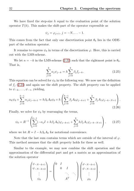
Similar to the example, we may now combine the shift operation and the
approximation of the differential part and get a matrix as an approximation of
the solution operator
⎛ ⎞ ⎛
⎞ ⎛ ⎞
0 I
⎜
⎝
ψ−N−k+1
ψ−N−k+2
.
ψ0
⎟
⎠ =
⎜
⎝
0 I
. ..
A T
⎟ ⎜
⎟ ⎜
⎟ ⎜
. .. ⎟ ⎜
⎠ ⎝
ϕ−N−k+1
ϕ−N−k+2
.
ϕ0
⎟
⎠ ,