The spectrum of delay-differential equations: numerical methods - KTH

40 Chapter 2. Computing the spectrum
Let x(t) be a solution to (2.35) and u(t, θ) := x(t + θ). We now have that
∂u
∂θ
= ∂u
∂t
since x(t + θ) is symmetric with respect to t and θ. It remains to show that
the boundary condition holds. Note that u ′ θ (t, 0) = ˙x(t), and hence u′ θ (t, 0) =
A0x(t) + A1x(t − τ) = A0u(t, 0) + A1u(t, −τ).
The converse is proven next. Suppose u(t, θ) is a solution to (2.36) and let
x(t) := u(t, 0) for t ≥ 0. From (2.36) it follows that ˙x(t) = u ′ t(t, 0) = u ′ θ (t, 0) =
A0u(t, 0) + A1u(t, −τ) = A0x(t) + A1x(t − τ). �
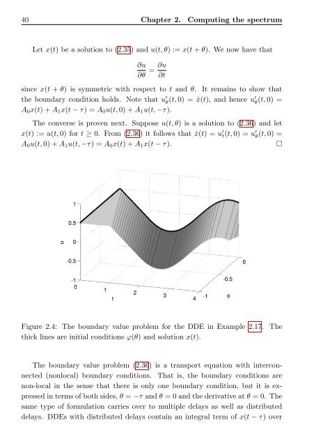
Figure 2.4: The boundary value problem for the DDE in Example 2.17. The
thick lines are initial conditions ϕ(θ) and solution x(t).
The boundary value problem (2.36) is a transport equation with interconnected
(nonlocal) boundary conditions. That is, the boundary conditions are
non-local in the sense that there is only one boundary condition, but it is expressed
in terms of both sides, θ = −τ and θ = 0 and the derivative at θ = 0. The
same type of formulation carries over to multiple delays as well as distributed
delays. DDEs with distributed delays contain an integral term of x(t − τ) over