The spectrum of delay-differential equations: numerical methods - KTH
The spectrum of delay-differential equations: numerical methods - KTH
The spectrum of delay-differential equations: numerical methods - KTH

You also want an ePaper? Increase the reach of your titles
YUMPU automatically turns print PDFs into web optimized ePapers that Google loves.
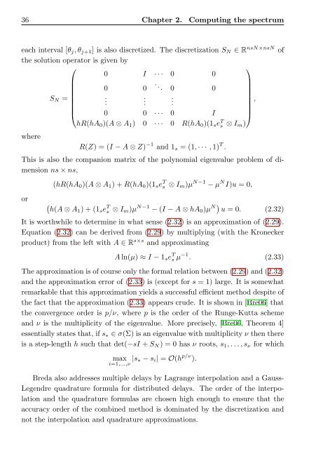
36 Chapter 2. Computing the <strong>spectrum</strong><br />
each interval [θj, θj+1] is also discretized. <strong>The</strong> discretization SN ∈ RnsN×nsN <strong>of</strong><br />
the solution operator is given by<br />
⎛<br />
⎞<br />
0 I · · · 0 0<br />
⎜<br />
. ⎟<br />
⎜ 0 0 .. 0 0 ⎟<br />
⎜<br />
SN = ⎜<br />
. . .<br />
⎟ ,<br />
. . .<br />
⎟<br />
⎜<br />
⎟<br />
⎝<br />
⎠<br />
where<br />
0 0 · · · 0 I<br />
hR(hA0)(A ⊗ A1) 0 · · · 0 R(hA0)(1se T s ⊗ Im)<br />
R(Z) = (I − A ⊗ Z) −1 and 1s = (1, · · · , 1) T .<br />
This is also the companion matrix <strong>of</strong> the polynomial eigenvalue problem <strong>of</strong> dimension<br />
ns × ns,<br />
or<br />
(hR(hA0)(A ⊗ A1) + R(hA0)(1se T s ⊗ Im)µ N−1 − µ N I)u = 0,<br />
� h(A ⊗ A1) + (1se T s ⊗ Im)µ N−1 − (I − A ⊗ hA0)µ N� u = 0. (2.32)<br />
It is worthwhile to determine in what sense (2.32) is an approximation <strong>of</strong> (2.29).<br />
Equation (2.32) can be derived from (2.29) by multiplying (with the Kronecker<br />
product) from the left with A ∈ R s×s and approximating<br />
A ln(µ) ≈ I − 1se T s µ −1 . (2.33)<br />
<strong>The</strong> approximation is <strong>of</strong> course only the formal relation between (2.29) and (2.32)<br />
and the approximation error <strong>of</strong> (2.33) is (except for s = 1) large. It is somewhat<br />
remarkable that this approximation yields a successful efficient method despite <strong>of</strong><br />
the fact that the approximation (2.33) appears crude. It is shown in [Bre06] that<br />
the convergence order is p/ν, where p is the order <strong>of</strong> the Runge-Kutta scheme<br />
and ν is the multiplicity <strong>of</strong> the eigenvalue. More precisely, [Bre06, <strong>The</strong>orem 4]<br />
essentially states that, if s∗ ∈ σ(Σ) is an eigenvalue with multiplicity ν then there<br />
is a step-length h such that det(−sI + SN) = 0 has ν roots, s1, . . . , sν for which<br />
max<br />
i=1,...,ν |s∗ − si| = O(h p/ν ).<br />
Breda also addresses multiple <strong>delay</strong>s by Lagrange interpolation and a Gauss-<br />
Legendre quadrature formula for distributed <strong>delay</strong>s. <strong>The</strong> order <strong>of</strong> the interpolation<br />
and the quadrature formulas are chosen high enough to ensure that the<br />
accuracy order <strong>of</strong> the combined method is dominated by the discretization and<br />
not the interpolation and quadrature approximations.