Chapter 6: Time Series Analysis

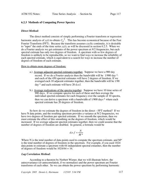
ATM 552 Notes: Time Series Analysis - Section 6a Page 1176.2.3 Methods of Computing Power SpectraDirect Method:The direct method consists of simply performing a Fourier transform or regressionharmonic analysis of y i (t) to obtain C k2 . This has become economical because of the FastFourier Transform (FFT). Because the transform assumes cyclic continuity, it is desirableto "taper" the ends of the time series y i (t), as will be discussed in section 6.2.5. When wedo a Fourier analysis we get estimates of the power spectrum at N/2 frequencies, but eachspectral estimate has only two degrees of freedom. A spectrum with so few degrees offreedom is unlikely to be reproducible, so we want to find ways to increase the reliability ofeach spectral estimate, which is equivalent to a search for ways to increase the number ofdegrees of freedom of each estimate.How to obtain more degrees of freedom:a.) Average adjacent spectral estimates together. Suppose we have a 900 dayrecord. If we do a Fourier analysis then the bandwidth will be 1/900 day -1 ,and each of the 450 spectral estimates will have 2 degrees of freedom. If weaveraged each 10 adjacent estimates together, then the bandwidth will be 1/90day -1 and each estimate will have 20 d.o.f.b.) Average realizations of the spectra together. Suppose we have 10 time series of900 days. If we compute spectra for each of these and then average theindividual spectral estimates for each frequency over the sample of 10 spectra,then we can derive a spectrum with a bandwidth of 1/900 days -1 where eachspectral estimate has 20 degrees of freedom.So how do we estimate the degrees of freedom in the direct – FFT method? If wehave N data points, and the resulting spectrum provides a variance at N/2 frequencies, wehave two degrees of freedom per spectral estimate. If we smooth the spectrum, then wemust estimate the effect of this smoothing on the degrees of freedom, which would beincreased. If we average adjacent spectral estimates together, then we could assume that thenumber of degrees of freedom are doubled. In general, a formula would bed.o.f = N M *Where N is the total number of data points used to compute the spectrum estimate, and M*is the total number of degrees of freedom in the spectrum. For example, if you used 1024data points to estimate a spectrum with 64 independent spectral estiamtes, then the numberof degrees of freedom would be 1024/64 = 16.Lag Correlation Method:According to a theorem by Norbert Wiener, that we will illustrate below, theautocovariance (or autocorrelation, if we normalize) and the power spectrum are Fouriertransforms of each other. So we can obtain the power spectrum by performing harmonicCopyright 2005 Dennis L. Hartmann 1/25/05 5:04 PM 117