Chapter 6: Time Series Analysis

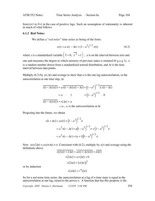
ATM 552 Notes: Time Series Analysis - Section 6a Page 104from k=1 to N-L in the case of positive lags. Such an assumption of stationarity is inherentin much of what follows.6.1.2 Red Noise:We define a “red noise” time series as being of the form:x(t) = ax(t t) +(1 a 2 ) 1/2 (t) (6.3)where x is a standardized variablex = 0, x' 2 =1, a is on the interval between zero andone and measures the degree to which memory of previous states is retained (0 < a < 1), is a random number drawn from a standardized normal distribution, and t is the timeinterval between data points.Multiply (6.3) by x(t-t) and average to show that a is the one-lag autocorrelation, or theautocorrelation at one time step, t.xtt ( )xt ()= ax( t t)xtt( )+ ( 1 a 2 ) 1/2 xtt ( )= a 1 + ( 1 a 2 ) 1/2 0xtt ( )xt ()= r( t) = a; i.e., a is the autocorrelation at tProjecting into the future, we obtainxt+ ( t)= ax()+ t ( 1 a 2 ) 1/2 = a 2 xtt ( )+ a 1 a 2( ) 1/2 + ( 1 a 2 ) 1/2 = a 2 xtt ( )+ ( a +1) ( 1 a 2 ) 1/2 Now x(t+2t) = ax(t+t) + . Consistent with (6.2), multiply by x(t) and average using thedefinitions above.xt ()xt+ ( 2t) = ax( t + t)xt()+ x()tr( 2t)= ar( t) + 0r( 2t)= ( r( t)) 2or by inductionrnt ( ) = r n ( t)So for a red noise time series, the autocorrelation at a lag of n time steps is equal to theautocorrelation at one lag, raised to the power n. A function that has this property is theCopyright 2005 Dennis L. Hartmann 1/25/05 5:04 PM 104