decision making with multiple imperfect decision makers - Institute of ...

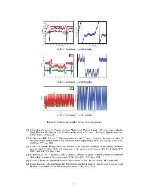
1.081.06108V 3Voltages1.041.0210.980.960.94V 1V 2Attacker’s move (m)6420−2−4−60.92−80.90 10 20 30 40 50 60 70 80 90 100Time step of game−100 10 20 30 40 50 60 70 80 90 100Time step of game(a) Level 0 defender vs. level 0 attacker1.11.08V1V2V343Voltages1.061.041.02Attacker’s move (m)21100.98−10.960 10 20 30 40 50 60 70 80 90 100Time step of game−20 10 20 30 40 50 60 70 80 90 100Time step of game(b) Level 1 defender vs. level 0 attacker1.15V1V2V3541.132Voltages1.0510.95VoltagesAttacker’s move (m) Attacker’s move (m)10−1−2−3−40.90 10 20 30 40 50 60 70 80 90 100Time step of game−50 10 20 30 40 50 60 70 80 90 100Time step of game(c) Level 0 defender vs. level 1 attackerFigure 4: Voltages and attacker moves of various games.[4] Ritchie Lee and David H. Wolpert. Decision Making with Multiple Imperfect Decision Makers, chapterGame Theoretic Modeling of Pilot Behavior during Mid-Air Encounters. Intelligent Systems ReferenceLibrary Series. Springer, 2011.[5] K. Tomsovic, D.E. Bakken, V. Venkatasubramanian, and A. Bose. Designing the next generation ofreal-time control, communication, and computations for large power systems. Proceedings of the IEEE,93(5):965 –979, may 2005.[6] Alvaro A. Cárdenas, Saurabh Amin, and Shankar Sastry. Research challenges for the security of controlsystems. In Proceedings of the 3rd conference on Hot topics in security, pages 6:1–6:6, Berkeley, CA,USA, 2008. USENIX Association.[7] K. Turitsyn, P. Sulc, S. Backhaus, and M. Chertkov. Options for control of reactive power by distributedphotovoltaic generators. Proceedings of the IEEE, 99(6):1063 –1073, june 2011.[8] Richard S. Sutton and Andrew G. Barto. Reinforcement Learning: An Introduction. MIT Press, 1998.[9] Lucian Busoniu, Robert Babuska, Bart De Schutter, and Ernst Damien. Reinforcement Learning andDynamic Programming Using Function Approximators. CRC Press, 2010.6