decision making with multiple imperfect decision makers - Institute of ...

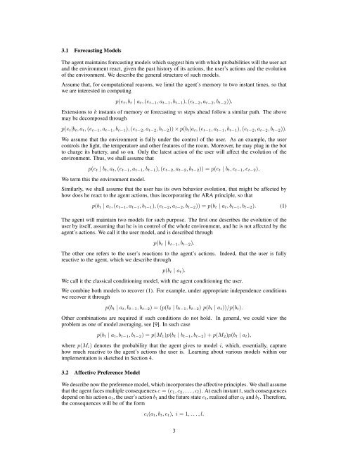
3.1 Forecasting ModelsThe agent maintains forecasting models which suggest him with which probabilities will the user actand the environment react, given the past history of its actions, the user’s actions and the evolutionof the environment. We describe the general structure of such models.Assume that, for computational reasons, we limit the agent’s memory to two instant times, so thatwe are interested in computingp(e t , b t | a t , (e t−1 , a t−1 , b t−1 ), (e t−2 , a t−2 , b t−2 )).Extensions to k instants of memory or forecasting m steps ahead follow a similar path. The abovemay be decomposed throughp(e t |b t , a t , (e t−1 , a t−1 , b t−1 ), (e t−2 , a t−2 , b t−2 )) × p(b t |a t , (e t−1 , a t−1 , b t−1 ), (e t−2 , a t−2 , b t−2 )).We assume that the environment is fully under the control of the user. As an example, the usercontrols the light, the temperature and other features of the room. Moreover, he may plug in the botto charge its battery, and so on. Only the latest action of the user will affect the evolution of theenvironment. Thus, we shall assume thatp(e t | b t , a t , (e t−1 , a t−1 , b t−1 ), (e t−2 , a t−2 , b t−2 )) = p(e t | b t , e t−1 , e t−2 ).We term this the environment model.Similarly, we shall assume that the user has its own behavior evolution, that might be affected byhow does he react to the agent actions, thus incorporating the ARA principle, so thatp(b t | a t , (e t−1 , a t−1 , b t−1 ), (e t−2 , a t−2 , b t−2 )) = p(b t | a t , b t−1 , b t−2 ). (1)The agent will maintain two models for such purpose. The first one describes the evolution of theuser by itself, assuming that he is in control of the whole environment, and he is not affected by theagent’s actions. We call it the user model, and is described throughp(b t | b t−1 , b t−2 ).The other one refers to the user’s reactions to the agent’s actions. Indeed, that the user is fullyreactive to the agent, which we describe throughp(b t | a t ).We call it the classical conditioning model, with the agent conditioning the user.We combine both models to recover (1). For example, under appropriate independence conditionswe recover it throughp(b t | a t , b t−1 , b t−2 ) = (p(b t | b t−1 , b t−2 ) p(b t | a t ))/p(b t ).Other combinations are required if such conditions do not hold. In general, we could view theproblem as one of model averaging, see [9]. In such casep(b t | a t , b t−1 , b t−2 ) = p(M 1 )p(b t | b t−1 , b t−2 ) + p(M 2 )p(b t | a t ),where p(M i ) denotes the probability that the agent gives to model i, which, essentially, capturehow much reactive to the agent’s actions the user is. Learning about various models within ourimplementation is sketched in Section 4.3.2 Affective Preference ModelWe describe now the preference model, which incorporates the affective principles. We shall assumethat the agent faces multiple consequences c = (c 1 , c 2 , . . . , c l ). At each instant t, such consequencesdepend on his action a t , the user’s action b t and the future state e t , realized after a t and b t . Therefore,the consequences will be of the formc i (a t , b t , e t ), i = 1, . . . , l.3