decision making with multiple imperfect decision makers - Institute of ...

The 2nd International Workshop onDECISION MAKING WITH MULTIPLE IMPERFECT DECISION MAKERSheld in conjunction with the 25 th Annual Conference on Neural Information Processing SystemsDecember 16, 2011, Sierra Nevada, Spain

© Institute of Information Theory and Automation 2011Printed in the Czech RepublicISBN 978-80-903834-6-3

The 2nd International Workshop onDECISION MAKING WITH MULTIPLEIMPERFECT DECISION MAKERSheld in conjunction with the 25th Annual Conference on Neural InformationProcessing Systems (NIPS 2011)December 16, 2011Sierra Nevada, Spainhttp://www.utia.cz/NIPSHomeOrganising and Programme CommitteeTatiana V Guy, Institute of Information Theory and Automation, Czech RepublicMiroslav Kárný, Institute of Information Theory and Automation, Czech RepublicDavid Rios Insua, Royal Academy of Sciences, SpainAlessandro E.P. Villa, University of Lausanne, SwitzerlandDavid Wolpert, Intelligent Systems Division, NASA Ames Research Center, USAThe partial support of Czech Science Foundation GA102/08/0567 is acknowledged.

Scope of the WorkshopPrescriptive Bayesian decision making supported by the efficient theoretically well-founded algorithms isknown to be a powerful tool. However, its application within multiple-participants’ settings needs anefficient support of imperfect participant (decision maker, agent), which is characterised by limited cognitive,acting and evaluative resources.The interacting and multiple-task-solving participants prevail in the natural (societal, biological) systems andbecome more and more important in the artificial (engineering) systems. Knowledge of conditions andmechanisms influencing the participant’s individual behaviour is a prerequisite to better understanding andrational improving of these systems. The diverse research communities permanently address these topicsfocusing either on theoretical aspects of the problem or (more often) on practical solution within a particularapplication. However, different terminology and methodologies used significantly impede furtherexploitation of any advances occurred. The workshop will bring the experts from different scientificcommunities to complement and generalise the knowledge gained relying on the multi-disciplinary wisdom.It extends the list of problems of the preceding NIPS workshop:How should we formalise rational decision making of a single imperfect decision maker? Does the answerchange for interacting imperfect decision makers? How can we create a feasible prescriptive theory forsystems of imperfect decision makers?The workshop especially welcomes contributions addressing the following questions:What can we learn from natural, engineered, and social systems? How emotions influence decision making?How to present complex prescriptive outcomes to the human? Do common algorithms really supportimperfect decision makers? What is the impact of imperfect designers of decision-making systems?The workshop aims to brainstorm on promising research directions, present relevant case studies andtheoretical results, and to encourage collaboration among researchers with complementary ideas andexpertise. The workshop will be based on invited talks, contributed talks and posters. Extensive moderatedand informal discussions ensure targeted exchange.List of Invited Talks• Automated Preferences ElicitationMiroslav Kárný, Tatiana V.Guy• Automated Explanations for MDP PoliciesOmar Zia Khan, Pascal Poupart, James P. Black• Modeling Humans as Reinforcement Learners: How to Predict Human Behavior in Multi˗ StageGamesRitchie Lee, David H. Wolpert, Scott Backhaus, Russell Bent, James Bono, Brendan Tracey• Random Belief LearningDavid Leslie• An Adversarial Risk Analysis Model for an Emotional Based Decision AgentJavier G. Rázuri, Pablo G. Esteban, David Rios Insua• Bayesian Combination of Multiple, Imperfect ClassifiersEdwin Simpson, Stephen Roberts, Ioannis Psorakis, Arfon Smith, Chris Lintott• Emergence of Reverse Hierarchies in Sensing and Planning by Optimizing Predictive InformationNaftali Tishby• Effect of Emotion on the Imperfectness of Decision MakingAlessandro E.P. Villa, Marina Fiori, Sarah Mesrobian, Alessandra Lintas,Vladyslav Shaposhnyk, Pascal Missonnier

Time Title Authors7:30—7:50 Opening session Organisers7:50—8:20 Emergence of Reverse Hierarchies in Sensing andPlanning by Optimizing Predictive InformationNaftali Tishby8:20—8:50 Modeling Humans as Reinforcement Learners:How to Predict Human Behavior in Multi-StageGames8:50—9:20 Coffee breakRitchie Lee, David H. Wolpert,Scott Backhaus, Russell Bent, James Bono,Brendan Tracey9:20—9:50 Automated Explanations for MDP Policies Omar Zia Khan, Pascal Poupart,James P. Black9:50—10:20 Automated Preference Elicitation Miroslav Kárný, Tatiana V.Guy10:20—10:40 Poster spotlights10:40—11:40 Posters and DemonstrationsArtificial Intelligence Design for Real-timeStrategy GamesDistributed Decision Making by Categorically-Thinking AgentsBayesian Combination of Multiple, ImperfectClassifiersDecision Making and Working Memory inAdolescents with ADHD after CognitiveRemediationTowards Distributed Bayesian Estimation:A Short Note on Selected AspectsVariational Bayes in Fully Probabilistic Controlfor Multi-Agent SystemsTowards a Supra-Bayesian Approach to Mergingof InformationIdeal and Non-Ideal Predictors in Estimation ofBellman FunctionDEMO: Interactive Two-Actors GameFiras Safadi, Raphael Fonteneau,Damien ErnstJoong Bum Rhim, Lav R. Varshney,Vivek K. GoyalEdwin Simpson, Stephen Roberts,Arfon Smith, Chris LintottMichel Bader, Sarah Leopizzi,Eleonora Fornari, Olivier Halfon,Nouchine HadjikhaniKamil Dedecius, Vladimíra SečkárováVáclav Šmídl, Ondřej TichýVladimíra SečkárováJan ZemanRitchie Lee11:45—4:00 BreakDEMO: AIsoy Robots4:00—4:30 Effect of Emotion on the Imperfectness ofDecision MakingDavid Rios InsuaAlessandro E. P. Villa, Marina Fiori,Sarah Mesrobian, Alessandra Lintas,Vladyslav Shaposhnyk, Pascal Missonnier4:30—5:00 Decision Support for a Social Emotional Robot Javier G. Rázuri, Pablo G. Esteban,David Rios Insua,5:00—6:00 Posters & Demonstrations and Coffee Break6:00—6:30 Random Belief Learning David Leslie6:30—7:00 Bayesian Combination of Multiple, ImperfectClassifiers7:00—8:00 Panel Discussion & Closing Remarks OrganisersEdwin Simpson, Stephen Roberts, IoannisPsorakis, Arfon Smith, Chris Lintott

Emergence of reverse hierarchies in sensing andplanning by optimizing predictive informationNaftali TishbyInterdisciplinary Center for Neural ComputationThe Ruth & Stan Flinkman family Chair in Brain ResearchThe Edmond and Lilly Safra Center for Brain Sciences, andSchool of Computer Science and EngineeringThe Hebrew University of Jerusalemtishby@cs.huji.ac.ilAbstractEfficient planning requires prediction of the future. Valuable predictions are basedon information about the future that can only come from observations of pastevents. Complexity of planning thus depends on the information the past of anenvironment contains about its future, or on the ”predictive information” of theenvironment. This quantity, introduced by Bilaek et. al., was shown to be subextensivein the past and future time windows, i.e.; to grow sub-linearly with thetime intervals, unlike the full complexity (entropy) of events which grow linearlywith time in stationary stochastic processes. This striking observation poses interestingbounds on the complexity of future plans, as well as on the required memoriesof past events. I will discuss some of the implications of this subextesivity ofpredictive information for decision making and perception in the context of pureinformation gathering (like gambling) and more general MDP and POMDP settings.Furthermore, I will argue that optimizing future value in stationary stochasticenvironments must lead to hierarchical structure of both perception and actionsand to a possibly new and tractable way of formulating the POMDP problem.1

Modeling Humans as Reinforcement Learners: Howto Predict Human Behavior in Multi-Stage GamesRitchie LeeCarnegie Mellon University Silicon ValleyNASA Ames Research Park MS23-11Moffett Field, CA 94035ritchie.lee@sv.cmu.eduScott BackhausLos Alamos National LaboratoryMS K764, Los Alamos, NM 87545backhaus@lanl.govDavid H. WolpertIntelligent Systems DivisionNASA Ames Research Center MS269-1Moffett Field, CA 94035david.h.wolpert@nasa.govRussell BentLos Alamos National LaboratoryMS C933, Los Alamos, NM 87545rbent@lanl.govJames BonoDepartment of EconomicsAmerican University4400 Massachusetts Ave. NWWashington DC 20016bono@american.eduBrendan TraceyDepartment of Aeronautics and AstronauticsStanford University496 Lomita Mall, Stanford, CA 94305btracey@stanford.eduAbstractThis paper introduces a novel framework for modeling interacting humans in amulti-stage game environment by combining concepts from game theory and reinforcementlearning. The proposed model has the following desirable characteristics:(1) Bounded rational players, (2) strategic (i.e., players account for oneanother’s reward functions), and (3) is computationally feasible even on moderatelylarge real-world systems. To do this we extend level-K reasoning to policyspace to, for the first time, be able to handle multiple time steps. This allows us todecompose the problem into a series of smaller ones where we can apply standardreinforcement learning algorithms. We investigate these ideas in a cyber-battlescenario over a smart power grid and discuss the relationship between the behaviorpredicted by our model and what one might expect of real human defendersand attackers.1 IntroductionWe present a model of interacting human beings that advances the literature by combining conceptsfrom game theory and computer science in a novel way. In particular, we introduce the firsttime-extended level-K game theory model [1, 2]. This allows us to use reinforcement learning (RL)algorithms to learn each player’s optimal policy against the level K − 1 policies of the other players.However, rather than formulating policies as mappings from belief states to actions, as in partiallyobservable Markov decision processes (POMDPs), we formulate policies more generally as mappingsfrom a player’s observations and memory to actions. Here, memory refers to all of a player’spast observations.This model is the first to combine all of the following characteristics. First, players are strategic inthe sense that their policy choices depend on the reward functions of the other players. This is in1

1S AS BS AU BU AS CS B2S AU AU AS BU BU B3S CS AS BS CU BU AS CFigure 1: An example semi Bayes net.Figure 2:Bayes net.An example iterated semicontrast to learning-in-games models whereby players do not use their opponents’ reward informationto predict their opponents’ decisions and to choose their own actions. Second, this approachis computationally feasible even on real-world problems. This is in contrast to equilibrium modelssuch as subgame perfect equilibrium and quantal response equilibrium [3]. This is also in contrast toPOMDP models (e.g. I-POMDP) in which players are required to maintain a belief state over spacesthat quickly explode. Third, with this general formulation of the policy mapping, it is straightforwardto introduce experimentally motivated behavioral features such as noisy, sampled or boundedmemory. Another source of realism is that, with the level-K model instead of an equilibrium model,we avoid the awkward assumption that players’ predictions about each other are always correct.We investigate all this for modeling a cyber-battle over a smart power grid. We discuss the relationshipbetween the behavior predicted by our model and what one might expect of real humandefenders and attackers.2 Game Representation and Solution ConceptIn this paper, the players will be interacting in an iterated semi net-form game. To explain an iteratedsemi net-form game, we will begin by describing a semi Bayes net. A semi Bayes net is a Bayesnet with the conditional distributions of some nodes left unspecified. A pictoral example of a semiBayes net is given in Figure 1. Like a standard Bayes net, a semi Bayes net consist of a set of nodesand directed edges. The ovular nodes labeled “S” have specified conditional distributions with thedirected edges showing the dependencies among the nodes. Unlike a standard Bayes net, there arealso rectangular nodes labeled “U” that have unspecified conditional dependencies. In this paper,the unspecified distributions will be set by the interacting human players. A semi net-form game,as described in [4], consists of a semi Bayes net plus a reward function mapping the outcome of thesemi Bayes net to rewards for the players.An iterated semi Bayes net is a Bayes net which has been time extended. It comprises of a semiBayes net (such as the one in Figure 1), which is replicated T times. Figure 2 shows the semi Bayesnet replicated three times. A set of directed edges L sets the dependencies between two successiveiterations of the semi Bayes net. Each edge in L connects a node in stage t − 1 with a node in staget as is shown by the dashed edges in Figure 2. This set of L nodes is the same between every twosuccessive stages. An iterated semi net-form game comprises of two parts: an iterated semi Bayesnet and a set of reward functions which map the results of each step of the semi Bayes net into anincremental reward for each player. In Figure 2, the unspecified nodes have been labeled “U A ” and“U B ” to specify which player sets which nodes.Having described above our model of the strategic scenario in the language of iterated semi net-formgames, we now describe our solution concept. Our solution concept is a combination of the level-Kmodel, described below, and reinforcement learning (RL). The level-K model is a game theoretic2

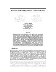
solution concept used to predict the outcome of human-human interactions. A number of studies[1, 2] have shown promising results predicting experimental data in games using this method. Thesolution to the level-K model is defined recursively as follows. A level K player plays as though allother players are playing at level K − 1, who, in turn, play as though all other players are playingat level K − 2, etc. The process continues until level 0 is reached, where the level 0 player playsaccording to a prespecified prior distribution. Notice that running this process for a player at K ≥ 2results in ricocheting between players. For example, if player A is a level 2 player, he plays asthough player B is a level 1 player, who in turn plays as though player A is a level 0 player playingaccording to the prior distribution. Note that player B in this example may not actually be a level 1player in reality – only that player A assumes him to be during his reasoning process.This work extends the standard level-K model to time-extended strategic scenarios, such as iteratedsemi net-form games. In particular, each Undetermined node associated with player i in the iteratedsemi net-form game represents an action choice by player i at some time t. We model player i’saction choices using the policy function, ρ i , which takes an element of the Cartesian product ofthe spaces given by the parent nodes of i’s Undetermined node to an action for player i. Note thatthis definition requires a special type of iterated semi-Bayes net in which the spaces of the parentsof each of i’s action nodes must be identical. This requirement ensures that the policy function isalways well-defined and acts on the same domain at every step in the iterated semi net-form game.We calculate policies using reinforcement learning (RL) algorithms. That is, we first define a level0 policy for each player, ρ 0 i . We then use RL to find player i’s level 1 policy, ρ1 i , given the level 0policies of the other players, ρ 0 −1, and the iterated semi net-form game. We do this for each player iand each level K. 13 Application: Cybersecurity of a Smart Power NetworkIn order to test our iterated semi net-form game modeling concept, we adopt a model for analyzingthe behavior of intruders into cyber-physical systems. In particular, we consider SupervisoryControl and Data Acquisition (SCADA) systems [5], which are used to monitor and control manytypes of critical infrastructure. A SCADA system consists of cyber-communication infrastructurethat transmits data from and sends control commands to physical devices, e.g. circuit breakers inthe electrical grid. SCADA systems are partly automated and partly human-operated. Increasingconnection to other cyber systems creating vulnerabilities to SCADA cyber attackers [6].Figure 3 shows a single, radial distribution circuit [7] from the transformer at a substation (node1) serving two load nodes. Node 2 is an aggregate of small consumer loads distributed along thecircuit, and node 3 is a relatively large distributed generator located near the end of the circuit. Inthis figure V i , p i , and q i are the voltage, real power, and reactive power at node i. P i , Q i , r i , andx i are the real power, reactive power, resistance and reactance of circuit segment i. Together, thesevalues represent the following physical system [7], where all terms are normalized by the nominalsystem voltage.P 2 = −p 3 , Q 2 = −q 3 , P 1 = P 2 + p 2 , Q 1 = Q 2 + q 2 (1)V 2 = V 1 − (r 1 P 1 + x 1 Q 1 ), V 3 = V 2 − (r 2 P 2 + x 2 Q 2 ) (2)In this model, r, x, and p 3 are static parameters, q 2 and p 2 are drawn from a random distributionat each step of the game, V 1 is the decision variable of the defender, q 3 is the decision variable ofthe attacker, and V 2 and V 3 are determined by the equations above. The injection of real powerp 3 and reactive power q 3 can modify the P i and Q i causing the voltage V 2 to deviate from 1.0.Excessive deviation of V 2 or V 3 can damage customer equipment or even initiate a cascading failurebeyond the circuit in question. In this example, the SCADA operator’s (defender’s) control over q 3is compromised by an attacker who seeks to create deviations of V 2 causing damage to the system.In this model, the defender has direct control over V 1 via a variable-tap transformer. The hardwareof the transformer limits the defenders actions at time t to the following domainD D (t) = 〈min(v max , V 1,t−1 + v), V 1,t−1 , max(v min , V 1,t−1 − v)〉1 Although this work uses level-K and RL exclusively, we are by no means wedded to this solution concept.Previous work on semi net-form games used a method known as Level-K Best-of-M/M’ instead of RL todetermine actions. This was not used in this paper because the possible action space is so large.3

VP 1, Q 1 1V P 2, Q 22V 3r 1, x 1r 2, x 2p 2, q 2p 3, q 3Figure 3: Schematic drawing of the three-node distribution circuit.where v is the voltage step size for the transformer, and v min and v max represent the absolute minand max voltage the transformer can produce. Similarly, the attacker has taken control of q 3 andits actions are limited by its capacity to produce real power, p 3,max as represented by the followingdomain.D A (t) = 〈−p 3,max , . . . , 0, . . . , p 3,max 〉Via the SCADA system and the attacker’s control of node 3, the observation spaces of the twoplayers includesΩ D = {V 1 , V 2 , V 3 , P 1 , Q 1 , M D }, Ω A = {V 2 , V 3 , p 3 , q 3 , M A }where M D and M A are used to denote each two real numbers that represent the respective player’smemory of the past events in the game. Both the defender and attacker manipulate their controls ina way to increase their own rewards. The defender desires to maintain a high quality of service bymaintaining the voltages V 2 and V 3 near the desired normalized voltage of one while the attacherwishes to damage equipment at node 2 by forcing V 2 beyond operating limits, i.e.( ) 2 ( ) 2 V2 − 1 V3 − 1R D = −−, R A = Θ[V 2 − (1 + ɛ)] + Θ[(1 − ɛ) − V 2 ]ɛɛHere, ɛ ∼ 0.05 for most distribution system under consideration, Θ is a Heaviside step function.Level 1 defender policy The level 0 defender is modeled myopically and seeks to maximize hisreward by following a policy that adjusts V 1 to move the average of V 2 and V 3 closer to one, i.e.(V 2 + V 3 )π D (V 2 , V 3 ) = arg min V1∈D D (t) − 12Level 1 attacker policy The level 0 attacker adopts a drift and strike policy based on intimateknowledge of the system. If V 2 < 1, we propose that the attacker would decrease q 3 by loweringit by one step. This would cause Q 1 to increase and V 2 to fall even farther. This policy achievessuccess if the defender raises V 1 in order to keep V 2 and V 3 in the acceptable range. The attackercontinues this strategy, pushing the defender towards v max until he can quickly raise q 3 to push V 2above 1 + ɛ . If the defender has neared v max , then a number of time steps will be required to forthe defender to bring V 2 back in range. More formally this policy can be expressed asLEVEL0ATTACKER()1 V ∗ = max q∈DA (t) |V 2 − 1|;2 if V ∗ > θ A3 then return arg max q∈DA (t) |V 2 − 1|;4 if V 2 < 15 then return q 3,t−1 − 1;6 return q 3,t−1 + 1;where θ A is a threshold parameter.3.1 Reinforcement Learning ImplementationUsing defined level 0 policies as the starting point, we now bootstrap up to higher levels by trainingeach level K policy against an opponent playing level K − 1 policy. To find policies that maximizereward, we can apply any algorithm from the reinforcement learning literature. In this paper, we use4

an ɛ-greedy policy parameterization (with ɛ = 0.1) and SARSA on-policy learning [8]. Trainingupdates are performed epoch-wise to improve stability. Since the players’ input spaces containcontinuous variables, we use a neural-network to approximate the Q-function [9]. We improveperformance by scheduling the exploration parameter ɛ in 3 segments during training: An ɛ of nearunity, followed by a linearly decreasing segment, then finally the desired ɛ.3.2 Results and DiscussionWe present results of the defender and attacker’s behavior at various level K. We note that ourscenario always had an attacker present, so the defender is trained to combat the attacker and has notraining concerning how to detect an attack or how to behave if no attacker is present. Notionally,this is also true for the attacker’s training. However in real-life the attacker will likely know thatthere is someone trying to thwart this attack.Level 0 defender vs. level 0 attacker The level 0 defender (see Figure 4(a)) tries to keep bothV 2 and V 3 close to 1.0 to maximize his immediate reward. Because the defender makes steps in V 1of 0.02, he does nothing for 30 < t < 60 because any such move would not increase his reward.For 30 < t < 60, the p 2 , q 2 noise causes V 2 to fluctuate, and the attacker seems to randomly driftback and forth in response. At t = 60, the noise plus the attacker and defender actions breaksthis “symmetry”, and the attacker increases his q 3 output causing V 2 and V 3 to rise. The defenderresponds by decreasing V 1 , indicated by the abrupt drops in V 2 and V 3 that break up the relativelysmooth upward ramp. Near t = 75, the accumulated drift of the level 0 attacker plus the responseof the level 0 defender pushes the system to the edge. The attacker sees that a strike would besuccessful (i.e., post-strike V 2 < 1 − θ A ), and the level 0 defender policy fails badly. The resultingV 2 and V 3 are quite low, and the defender ramps V 1 back up to compensate. Post strike (t >75), the attackers threshold criterion tells him that an immediate second strike would would not besuccessful, however, this shortcoming will be resolved via level 1 reinforcement learning. Overall,this is the behavior we have built into the level 0 players.Level 1 defender vs. level 0 attacker During the level 1 training, the defender likely experiencesthe type of attack shown in Figure 4(a) and learns that keeping V 1 a step or two above 1.0 is a goodway to keep the attacker from putting the system into a vulnerable state. As seen in Figure 4(b), thedefender is never tricked into performing a sustained drift because the defender is willing to takea reduction to his reward by letting V 3 stay up near 1.05. For the most part, the level 1 defender’sreinforcement learning effectively counters the level 0 attacker drift-and-strike policy.Level 0 defender vs. level 1 attacker The level 1 attacker learning sessions correct a shortcomingin the level 0 attacker. After a strike (V 2 < 0.95 in Figure 4(a)), the level 0 attacker drifts up fromhis largest negative q 3 output. In Figure 4(c), the level 1 attacker anticipates that the increase in V 2when he moves from m = −5 to m = 5 will cause the level 0 defender to drop V 1 on the next move.After this drop, the level 1 attacker also drops from m = +5 to −5. In essence, the level 1 attackeris leveraging the anticipated moves of the level 0 defender to create oscillatory strikes that push V 2below 1 − ɛ nearly every cycle.AcknowledgmentsThis research was supported by the NASA Aviation Safety Program SSAT project, and the LosAlamos National Laboratory LDRD project Optimization and Control Theory for Smart Grid.References[1] Miguel Costa-Gomes and Vincent Crawford. Cognition and behavior in two-person guessing games: Anexperimental study. American Economic Review, 96(5):1737–1768, December 2006.[2] Dale O. Stahl and Paul W. Wilson. On players’ models of other players: Theory and experimental evidence.Games and Economic Behavior, 10(1):218 – 254, 1995.[3] Richard Mckelvey and Thomas Palfrey. Quantal response equilibria for extensive form games. ExperimentalEconomics, 1:9–41, 1998. 10.1023/A:1009905800005.5

1.081.06108V 3Voltages1.041.0210.980.960.94V 1V 2Attacker’s move (m)6420−2−4−60.92−80.90 10 20 30 40 50 60 70 80 90 100Time step of game−100 10 20 30 40 50 60 70 80 90 100Time step of game(a) Level 0 defender vs. level 0 attacker1.11.08V1V2V343Voltages1.061.041.02Attacker’s move (m)21100.98−10.960 10 20 30 40 50 60 70 80 90 100Time step of game−20 10 20 30 40 50 60 70 80 90 100Time step of game(b) Level 1 defender vs. level 0 attacker1.15V1V2V3541.132Voltages1.0510.95VoltagesAttacker’s move (m) Attacker’s move (m)10−1−2−3−40.90 10 20 30 40 50 60 70 80 90 100Time step of game−50 10 20 30 40 50 60 70 80 90 100Time step of game(c) Level 0 defender vs. level 1 attackerFigure 4: Voltages and attacker moves of various games.[4] Ritchie Lee and David H. Wolpert. Decision Making with Multiple Imperfect Decision Makers, chapterGame Theoretic Modeling of Pilot Behavior during Mid-Air Encounters. Intelligent Systems ReferenceLibrary Series. Springer, 2011.[5] K. Tomsovic, D.E. Bakken, V. Venkatasubramanian, and A. Bose. Designing the next generation ofreal-time control, communication, and computations for large power systems. Proceedings of the IEEE,93(5):965 –979, may 2005.[6] Alvaro A. Cárdenas, Saurabh Amin, and Shankar Sastry. Research challenges for the security of controlsystems. In Proceedings of the 3rd conference on Hot topics in security, pages 6:1–6:6, Berkeley, CA,USA, 2008. USENIX Association.[7] K. Turitsyn, P. Sulc, S. Backhaus, and M. Chertkov. Options for control of reactive power by distributedphotovoltaic generators. Proceedings of the IEEE, 99(6):1063 –1073, june 2011.[8] Richard S. Sutton and Andrew G. Barto. Reinforcement Learning: An Introduction. MIT Press, 1998.[9] Lucian Busoniu, Robert Babuska, Bart De Schutter, and Ernst Damien. Reinforcement Learning andDynamic Programming Using Function Approximators. CRC Press, 2010.6

Automated Explanations for MDP PoliciesOmar Zia Khan, Pascal Poupart and James P. BlackDavid R. Cheriton School of Computer ScienceUniversity of Waterloo200 University Avenue West, Waterloo, ON, N2L 3G1, Canada{ozkhan, ppoupart, jpblack}@cs.uwaterloo.caAbstractExplaining policies of Markov Decision Processes (MDPs) is complicated dueto their probabilistic and sequential nature. We present a technique to explainpolicies for factored MDP by populating a set of domain-independent templates.We also present a mechanism to determine a minimal set of templates that, viewedtogether, completely justify the policy. We demonstrate our technique using theproblems of advising undergraduate students in their course selection and evaluateit through a user study.1 IntroductionSequential decision making is a notoriously difficult problem especially when there is uncertainty inthe effects of the actions and the objectives are complex. MDPs [10] provide a principled approachfor automated planning under uncertainty. State-of-the-art techniques provide scalable algorithmsfor MDPs [9], but the bottleneck is gaining user acceptance as it is harder to understand why certainactions are recommended. Explanations can enhance the user’s understanding of these plans (whenthe policy is to be used by humans like in recommender systems) and help MDP designers to debugthem (even when the policy is to be used by machines, like in robotics). Our explanations highlightkey factors through a set of explanation templates. The set of templates are sufficient, such that theyjustify the recommended action, yet also minimal, such that the size of the set cannot be smaller. Wedemonstrate our technique through a course-advising MDP and evaluate our explanations through auser study. A more detailed description of our work can be found in [6].2 BackgroundA Markov decision process (MDP) is defined by a set S of states s, a set A of actions a, a transitionmodel (the probability P r (s ′ |s, a) of an action a in state s leading to state s ′ ), a reward model (theutility/reward R (s, a) for executing action a in state s), and a discount factor γ ∈ [0, 1). FactoredMDPs [1] are typically used for MDPs with large state space where states are determined by valuesof some variables. A scenario sc is defined as the set of states obtained by assigning values to asubset of state variables. A policy π : S → A is a mapping from states to actions. The value V π (s)of a policy π when starting in state s is the sum of the expected discounted rewards earned byexecuting policy π. A policy can be evaluated by using Bellman’s equation V π (s) = R (s, π (s)) +γ ∑ s ′ ∈S P r (s′ |s, π (s)) · V π (s ′ ). We shall use an alternative method to evaluate a policy basedon occupancy frequencies. The discounted occupancy frequency (hereafter referred as occupancyfrequency) λ π s 0(s ′ ) is the expected (discounted) number of times we reach state s ′ from starting states 0 by executing policy π. Occupancy frequencies can be computed by solving Eq. 1.λ π s 0(s ′ ) = δ (s ′ , s 0 ) + γ ∑ s∈SP r (s ′ |s, π (s)) · λ π s 0(s) ∀s ′ (1)1

where δ (s ′ , s 0 ) is a Kroenecker delta which assigns 1 when s ′ = s 0 and 0 otherwise. The occupancyfrequencies for a scenario (or a set of scenarios), λ π s 0(sc), is the expected number of times we reacha scenario sc, from starting state s 0 , by executing policy π i.e., λ π s 0(sc) = ∑ s∈sc λπ s 0(s). Let sc rbe a set of scenarios with reward value r. The dot product of occupancy frequencies and rewardsgives the value of a policy, as shown in Eq. 2.V π (s 0 ) = ∑ rλ π s 0(sc r ) · r (2)An optimal policy π ∗ earns the highest value for all states (i.e., V π∗ (s) ≥ V π (s) ∀π, s).3 Explanations for MDPs3.1 Templates for ExplanationsOur explanation answers the question, “Why has this action been recommended?” by populatinggeneric templates, at run-time, with domain-specific information from the MDP i.e., occupancyfrequency of a scenario. The reward function implicitly partitions the state space in regions withequal reward value. These regions can be defined as partial variable assignments corresponding toscenarios or sets of scenarios. An explanation then could be the frequency of reaching a scenariois highest (or lowest). This is especially useful when this scenario also has a relatively high (orlow) reward. Below we describe templates in which the underlined phrases (scenarios and theirfrequencies) are populated at run-time.• Template 1: “ActionName is the only action that is likely to take you toV ar 1 = V al 1 , V ar 2 = V al 2 , ... about λ times, which is higher (or lower) than any otheraction”• Template 2: “ActionName is likely to take you to V ar 1 = V al 1 , V ar 2 = V al 2 , ... aboutλ times, which is as high (or low) as any other action”• Template 3: “ActionName is likely to take you to V ar 1 = V al 1 , V ar 2 = V al 2 , ... aboutλ times”While these templates provide a method to present explanations, multiple templates can be populatedeven for non-optimal actions; a non-optimal action can have the highest frequency of reaching ascenario without having the maximum expected utility. Thus, we need to identify a set of templatesthat justify the optimal action.3.2 Minimal Sufficient ExplanationsWe define an explanation as sufficient if it can prove that the recommendation is optimal, i.e., theselected templates show the action is optimal without needing additional templates. A sufficient explanationcannot be generated for a non-optimal action since an explanation for another action (e.g.,the optimal action) will have a higher utility. A sufficient explanation is also minimal if it includesthe minimum number of templates needed to ensure it is sufficient. The minimality constraint isuseful for users and sufficiency constraint is useful for designers.Let s 0 be the state where we need to explain why π ∗ (s 0 ) is an optimal action. We can compute thevalue of the optimal policy V π∗ (s 0 ) or the Q-function 1 Q π∗ (s 0 , a) using Eq. 2. Since a template ispopulated by a frequency and a scenario, the utility of this pair in a template is λ π∗s 0(sc r ) · r. Let Ebe the set of frequency-scenario pairs that appear in an explanation. If we exclude a pair from theexplanation, the utility is λ π∗s 0(sc i ) · ¯r, where r min is the minimum value for the reward variable.This definition indicates that the worst is assumed for the scenario in this pair. The utility of anexplanation V E is1 In reinforcement learning, the Q-function Q π (s, a) denotes the value of executing action a in state sfollowed by policy π.2

V E = ∑ i∈Eλ π∗s 0(sc i ) · r i + ∑ λ π∗s 0(sc j ) · r min (3)j /∈Ewhere the first part includes the utility from all the pairs in the explanation and the second partconsiders the worst case for all other pairs. For an explanation to be sufficient, its utility has tobe higher than the next best action, i.e., V π∗ ≥ V E > Q π∗ (s 0 , a) ∀a ≠ π ∗ (s 0 ). For it to beminimal, it should use the fewest possible pairs. Let us define the gain of including a pair in anexplanation as the difference between the utility of including versus excluding that pair (λ π∗s 0(sc i ) ·r i − λ π∗s 0(sc i ) · r min ). To find a minimal sufficient explanation, we can sort the gains of all pairsin descending order and select the first k pairs that ensure V E ≥ Q π∗ (s 0 , a). This provides ourminimal sufficient explanation.3.3 Workflow and AlgorithmThe designer identifies the states and actions, and specifies the transition and reward functions. Theoptimal policy is computed, using a technique such as value iteration, and is consulted to determinethe optimal action. Now an explanation can be requested. The pseudo code for the algorithm tocompute a minimal sufficient explanation is shown in Algorithm 1.Algorithm 1 Computing Minimal Sufficient ExplanationsThe function ComputeScenarios returns the set of scenarios with reward value r which is availablein the encoding of the reward function. The function ComputeOccupancyFrequency isthe most expensive step which corresponds to solging the system of linear system defined in Eq. 1,which has a worst case complexity that is cubic in the size of the state space. However, in practice,the running time can often be sublinear by using variable elimination to exploit conditionalindependence and algebraic decision diagrams [5] to automatically aggregate states with identicalvalues/frequencies. The function GenerateTemplates chooses an applicable template, fromthe list of templates, in the order of the list, with the last always applicable.4 Experiments and Evaluation4.1 Sample ExplanationsWe ran experiments on course-advising and hand-washing MDPs [6]. We only discuss the courseadvisingdomain here due to space considerations. The transition model was obtained by usinghistorical data collected over several years at the University of Waterloo. The reward function providesrewards for completing different degree requirements. The horizon of this problem is 3 steps,3

each step representing one term and the policy emits a pair of courses to take in that term. Theproblem has 117.4 million states. We precomputed the optimal policy since it does not need to berecomputed for every explanation. We were able to compute explanations in approximately 1 secondon a Pentium IV 1.66 GHz laptop with 1GB RAM using Java on Windows XP with the optimalpolicy and second best action precomputed. A sample explanation is shown below.• Action TakeCS343&CS448 is the best action because:-– It’s likely to take you to CoursesCompleted = 6, T ermNumber = F inal about0.86 times, which is as high as any other action4.2 User Study with StudentsWe conducted a user study to evaluate explanations for course advising. We recruited 37 studentsand showed 3 different recommendations with explanations for different states. For each explanation,they were asked to rate it on various factors such as comprehension, trust-worthiness andusefulness with partial results shown in Figure 1. 59% (65/111) of the respondents indicated thatthey were able to understand our explanation without any other information; the rest also wanted toknow the occupancy frequencies for some other actions. We can provide this information as it isalready computed. 76% (84/111) believed that the explanation provided by our system was accurate,with a few wanting to know our sample size to judge the accuracy. 69% (77/111) indicated that theywould require extra information beyond that presented in the explanation. When asked what othertype of information is needed, we discovered that they wanted the model to cater to preferences suchas student’s interest, future career plans, and level of difficulty rather than the explanation being inadequatefor our existing model. An important indicator of the usefulness of these explanations isthat 71% (79/111) of the students mentioned that the explanation provided them with extra informationthat helped them in making a decision. Also while some students, 23% (26/111), initiallydisagreed with the recommendation, in 35% (9/26) of these cases our explanation convinced themto change their mind and agree with the original recommendation. The rest disagreed primarilybecause they wanted a more elaborate model, so no explanation could have convinced them.We also asked students if they were provided with our system, in addition to the option of discussingtheir choices with an undergraduate advisor, would they use it. 86% of them mentioned they woulduse it from home and 89% mentioned they would use it before meeting with an advisor to examinedifferent options for themselves. These numbers indicate substantial interest in our explanations.The explanations generated by our system are generic, while those provided by the advisors aredomain-specific. The user study indicates that these two types of explanations are complementaryand students would like to access our explanations in addition to consulting advisors.5 Relationship to Other Explanations StrategiesExplanations have been considered an essential component of intelligent reasoning systems and variousstrategies have been devised to generate them. Explanations for expert systems are generallyin the form of execution traces, such as in MYCIN [2]. Execution traces indicate the rules used inarriving at a conclusion. There are no specific rules in an MDP and the optimal decision is madeby maximizing the expected utility which involves considering all of the transition and reward function.Thus, in our explanation we highlight the more important parts of the transition and rewardfunction. Xplain [12] is an example of an intelligent tutoring system that also provided justificationsof its decisions. In addition to the rules used by the expert system, it also needed additionaldomain knowledge to generate these explanations. Our current approach does not use any additionaldomain knowledge, however this also means we cannot justify the correctness of the transition orreward function. We can only argue about the optimal action using the specified transition and rewardfunctions. Explanations in single-shot recommender systems [13] and case-based reasoningsystems [11] are typically based on identifying similar clusters of users or cases and then demonstratingthe similarity of the current choice to a cluster or case. Since MDPs are not based on theprinciple of recommending actions based on similarity, such an approach to generate explanationswould be infeasible. Herlocker et al. [4] presented the idea of highlighting key data leading to arecommendation for explanations in recommender systems. Our approach is also motivated by thisidea with the key difference that choices in MDPs also impact future states and actions rather than4

Figure 1: User Perception of MDP-Based Explanationsexplaining an isolated decision. McGuinness et al. [8] identify several templates to present explanationsin task processing systems based on predefined workflows. Our approach also uses templates,but we cannot use predefined workflows due to the probabilistic nature of MDPs.Lacave et al. [7] presented several approaches to explain graphical models, including Bayesian networksand influence diagrams. Their explanations require a background in decision analysis andthey present utilities of different actions graphically and numerically. We focus on users withoutany knowledge of utility theory. Elizalde et al. [3] present an approach to generate explanations foran MDP policy that recommends actions for an operator in training. A set of explanations is definedmanually by an expert and their algorithm determines a relevant variable to be presented as explanation.Our approach does not restrict to a single relevant variable and considers the long-term effectsof the optimal action (beyond one time step). We also use generic, domain-independent templatesand provide a technique to determine a minimum set of templates that can completely justify anaction.6 Significance and ImplicationsWhile there has been a lot of work on explanations for intelligent systems, such as expert, rule-based,and case-based reasoning systems, there has not been much work for probabilistic and decisiontheoreticsystems. The main reason behind this discrepancy is the difference in processes throughwhich they arrive at their conclusions. For probabilistic and decision-theoretic systems, there arewell-known axioms of probability and theorems from utility theory that are applied to perform inferenceor compute a policy. Therefore, experts do not need to examine the reasoning trace todetermine if the inference or policy computation process is correct. The trace would essentially referto concepts such as Bayes’ theorem, or the principle of maximum expected utility etc, which donot need to be verified. Instead, the input, i.e., transition and reward function, need to be verified.With recent advances in scalability and the subsequent application of MDPs to real-world problems,now explanation capabilities are needed. The explanation should highlight portions of the input thatlead to a particular result.Real-world MDPs are difficult to design because they can involve millions of states. There areno existing tools for experts to examine and/or debug their models. The current design processinvolves successive iterations of tweaking various parameters to achieve a desirable output. At theend, the experts still cannot verify if the policy indeed accurately reflects their requirements. Ourexplanations provide hints to experts in debugging by indicating the components of the model thatare being utilized in the decision-making process at the current step. This allows experts to verifywhether the correct components are being used and focus the tweaking of the model.5

Current users have to trust an MDP policy blindly, with no explanations whatsoever regarding theprocess of computing the recommendation or the confidence of the system in this recommendation.They cannot observe which factors have been considered by the system while making the recommendation.Our explanations can provide users with the information that the MDP is using to baseits recommendation. This is especially important if user preferences are not accurately encoded.If experts or users disagree with the optimal policy, the next step would be to automatically updatethe model based on interaction, i.e., update the transition and reward functions if the user/expertdisagree with the optimal policy despite the explanation. Any such automatic update of the modelneeds to be preceded by a proper understanding of the existing model, which can only be achievedthrough explanations, such as those provided by our system.Just like the optimal policies for MDPs from different domains can be computed using the sameunderlying techniques, our technique to generate explanations is also generic and can be employedfor an MDP from any domain. We have used the same approach described here to generate minimalsufficient explanations for the handwashing MDP [6]. The mechanism to present the explanation tousers can then be tailored for various domains. Often a fancier graphical presentation may be moreuseful than a text-based template. Our focus is to produce generic explanations that can then betransformed for presentation in a user-friendly format.7 ConclusionWe presented a mechanism to generate explanations for factored MDP in any domain without requiringany additional effort from the MDP designer. We introduced the concept of a minimalsufficient explanation through which an action can be explained using the fewest possible templates.We showed that our explanations can be generated in near-real time and conducted a user study toevaluate their effectiveness. The students appreciated the extra information provided by our genericexplanations. Most of the students considered the combination of our explanation with the advisorexplanation more effective than either one alone.In the future, it would be interesting to extend this work to partially observable MDPs. Since thestates are not directly observable, it is not obvious how one could generate an explanation that refersto the frequency with which some states are visited. It would also be interesting to extend this workto reinforcement learning problems where the parameters of the model (i.e., transition probabilitiesand reward function) are unknown or at best partially known. Finally, when an explanation is providedand the user insists that the recommended action is suboptimal, then it would be interesting toclose the loop by updating the model to take into account the feedback provided by the user.References[1] Craig Boutilier, Richard Dearden, and Moisés Goldszmidt. Stochastic dynamic programmingwith factored representations. Artificial Intelligence, 121(1-2):49–107, 2000.[2] W. J. Clancey. The epistemology of a rule-based expert system – a framework for explanation.Artificial Intelligence, 20:215–251, 1983.[3] F. Elizalde, E. Sucar, A. Reyes, and P. deBuen. An MDP approach for explanation generation.In AAAI Workshop on Explanation-Aware Computing, 2007.[4] J. Herlocker. Explanations in recommender systems. In CHI’ 99 Workshop on Interacting withRecommender Systems, 1999.[5] Jesse Hoey, Robert St-aubin, Alan Hu, and Craig Boutilier. SPUDD: Stochastic planning usingdecision diagrams. In UAI, pages 279–288, Stockholm, Sweden, 1999.[6] Omar Zia Khan, Pascal Poupart, and James P. Black. Minimal sufficient explanations forfactored markov decision processes. In ICAPS, Thessaloniki, Greece, 2009.[7] C. Lacave, M. Luque, and F.J. Dez. Explanation of Bayesian networks and influence diagramsin Elvira. IEEE Transactions on Systems, Man, and Cybernetics, 37(4):952–965, 2007.[8] D. McGuinness, A. Glass, M. Wolverton, and P. da Silva. Explaining task processing in cognitiveassistants that learn. In Proceedings of AAAI Spring Symposium on Interaction Challengesfor Intelligent Assistants, 2007.6

[9] Warren B. Powell. Approximate Dynamic Programming: Solving the Curses of Dimensionality.Wiley, 2nd edition, 2011.[10] Martin Puterman. Markov Decision Processes. Wiley, 1994.[11] Frode Sørmo, Jörg Cassens, and Agnar Aamodt. Explanation in case-based reasoning—perspectives and goals. Artificial Intelligence Review, 24(2):109–143, 2005.[12] W. R. Swartout. Xplain: A system for creating and explaining expert consulting programs.Artificial Intelligence, 21:285–325, 1983.[13] N. Tintarev and J. Masthoff. A survey of explanations in recommender systems. In ICDEWorkshop on Recommender Systems & Intelligent User Interfaces, 2007.7

Automated Preferences ElicitationMiroslav KárnýDepartment of Adaptive SystemsInstitute of Information Theory and AutomationAcademy of Sciences of the Czech RepublicPod vodárenskou věží 4, 182 08 Prague 8, Czech Republicschool@utia.cas.czTatiana V. GuyDepartment of Adaptive SystemsInstitute of Information Theory and AutomationAcademy of Sciences of the Czech RepublicPod vodárenskou věží 4, 182 08 Prague 8, Czech Republicguy@utia.cas.czAbstractSystems supporting decision making became almost inevitable in the moderncomplex world. Their efficiency depends on the sophisticated interfaces enablinga user take advantage of the support while respecting the increasing on-line informationand incomplete, dynamically changing user’s preferences. The best decisionmaking support is useless without the proper preference elicitation. The paperproposes a methodology supporting automatic learning of quantitative descriptionof preferences. The proposed elicitation serves to fully probabilistic design, whichis an extension of Bayesian decision making.1 IntroductionA feasible and effective solution of preference elicitation problem decides on the efficiency of anyintelligent system supporting decision making. Indeed, to recommend a participant 1 an optimal sequenceof optimal decisions requires knowing some information about what the participant (affectedby the recommended decision, if accepted) considers as “optimal”. Extracting the information aboutthe participant’s preferences or utility is known as preference elicitation or utility elicitation 2 . Thisvital problem has been repeatedly addressed within artificial intelligence, game theory, operationresearch and many sophisticated approaches have been proposed [7], [8], [6], [5]. A number ofapproaches has arisen in connection with applied sciences like economy, social science, clinicaldecision making, transportation, see, for instance, [18], [9]. To ensure feasibility and practical applicability,many decision support systems have been designed under various assumptions on thestructure of preferences. In particular, a broadly accepted additive independence [16] of values ofindividual attributes is not generally valid. In many applications the preferences of attributes aremostly dependent and the assumption above significantly worsens the elicitation results 3 .To benefit from any decision support, the preferences should be known in the form allowing theirprocessing by an intended decision support system. Unless the participant’s preferences are completelyprovided by the participant, they should be learned from either past data or domain-specific1 Participant is also known as user, decision maker, agent.2 The term utility generally has a bit different coverage within decision-making context.3 The assumption can be weakened by a introducing a conditional preferential independence, [4].1

information (technological knowledge, physical laws, etc.). Eliciting the needed information itself isinherently hard task, which success depends on experience and skills of an elicitation expert. Preferencescan be elicited from past data directly collected on the underlying decision-making process orfrom indirect data learned from a number of similar situations. Despite acquiring the probabilisticinformation from data is well-elaborated, learning can be hard, especially when the space of possiblebehaviour is larger than that past data cover. Then the initial preferences for the remaining part ofthe behaviour should be properly assigned.The process of eliciting of the domain-specific information is difficult, time-consuming and errorpronetask 4 . Domain experts provide subjective opinions, typically expressed in different and incompatibleforms. The elicitation expert should elaborate these opinions into a distribution describingpreferences in a consistent way. Significant difficulties emerge when competitive/complementingopinions with respect to the same collection of attributes should be merged. A proper merging theirindividual opinions within a high-dimensional space of possible behaviour is unfeasible. Besidesdomain experts having domain-specific information are often unable to provide their opinion on apart of behaviour due to either limited knowledge of the phenomenon behind or the indifferencetowards the possible instances of behaviour. Then, similarly to the learning preferences from pastdata, the optimal strategy heavily depends on the initial preferences assigned to the part of behaviournot “covered” by the domain-specific information.Process of eliciting information itself requires significant cognitive and computational effort of theelicitation expert. Even if we neglect the cost of this effort 5 , the elicitation result is always verylimited by the expert’s imperfection, i.e. his inability to devote an infinite deliberation effort toeliciting. Unlike imperfection of experts providing domain-specific information, imperfection ofelicitation experts can be eliminated. This motivate the search for a feasible automated support ofpreference elicitation, that does not rely on any elicitation expert.The dynamic decision making strengthes the dependence on the preference elicitation. Indeed, theparticipant acting within a dynamically changing environment with evolving parameters may graduallychange preferences. The intended change may depend on the future behaviour. The overalltask is going harder when participant interacts with other dynamic imperfect participants within acommon environment.The paper concerns a construction of probabilistic description of preferences based on the informationavailable. Dynamic decision making under uncertainty from the perspective of an imperfectparticipant is considered. The participant solves DM task with respect to its environment and basedon a given finite set of opinions gained from providers of domain expertise or learned from the pastdata or both. The set indirectly represents the preferences in a non-unique way 6 . Additionally, theparticipant may be still uncertain about the preferences on a non-empty subset of behaviour. To designan optimal strategy, a participant employs Fully Probabilistic Design (FPD) of DM strategies,[10, 12] whose specification relies on the notion of an ideal closed-loop model which is essentiallya probabilistic description of the preferences. In other words, an ideal closed-loop model describesthe closed-loop behaviour, when the participant’s DM strategy is optimal. FPD searches for the optimalstrategy by minimising the divergence of the current closed-loop description on the ideal one.Adopted FPD implies availability of probabilistic description of the environment and probabilisticdescription of the past closed-loop data.Section 2 specifies assumptions under which the automated preference elicitation is proposed withinthe considered FPD. Section 3 describes construction of the ideal closed-loop distribution based onthe information provided. The proposed solution is discussed in Section 4 followed by the concludingremarks in Section 5.4 It should be mentioned that practical solutions mostly use a laborious and unreliable process of manualtuning a number of parameters of the pre-selected utility function. Sometimes the high number of parametersmakes this solution unfeasible. Then there are attempts to decrease the number of parameters to reach anacceptable feasibility level.5 This effort is usually very high and many sophisticated approaches aim at optimising a trade-off betweenelicitation cost and value of information it provides (often decision quality is considered), see for instance [3].6 Even, when we identify instances of behaviour that cannot be distinguished from the preferences’ viewpoint.2

2 AssumptionsThe considered participant deals with a DM problem, where the reached decision quality is expressedin terms of a l a -tuple of attributes a = (a 1 , . . . , a la ) ∈ a = ∏ lai=1 a i , l a < ∞. ∏ denotesCartesian product of sets a i the respective attribute entries belong to. The occurrence of attributesdepends on an optional l d -dimensional decision d = (d 1 , . . . , d ld ) ∈ d = ∏ ldj=1 d j , l d < ∞. In theconsidered preference elicitation problem, the following assumptions are adopted.A1 The participant is able to specify its preferences on the respective entries of attributes a i ∈ a isuch that the most preferred value of each attribute is uniquely defined. For convenience,let the best attribute value be zero.A2 The participant has at disposal a probabilistic model M(a|d), which is the probability density(pd 7 ) of the attributes a conditioned on decisions d. The support of M(a|d) is assumed toinclude (a, d).A3 The participant has 8 a joint pd P(a, d), describing behaviour (a, d) of the closed loop formedby the acting participant and by its environment 9 . The support of P(a, d) is assumed toinclude (a, d).A4 The participant uses fully probabilistic design (FPD), [12], of decision-making strategies. FPDconsiders a specification of the ideal pd I(a, d) assigning high values to desired pairs(a, d) ∈ (a, d) and small values to undesired ones. The optimal randomised strategyS opt (d) is selected among strategy-describing pds S ∈ S as a minimiser of the Kullback-Leibler divergence (KLD, [17])∫( )M(a|d)S(d)S opt ∈ Arg min M(a|d)S(d) lnd(a, d) = Arg minSI(a, d)D(MS||I).S(a,d)Note that the use of FPD represents no constraints as for a classical preference-quantifying utilityU(a, d) : (a, u) → [−∞, ∞) it suffices to consider the ideal pd of the formI(a, d) =∫(a,d)M(a|d) exp(U(a, d)/λ)λ > 0.M(a|d) exp(U(a, d)/λ) d(a, d),Then, the FPD with such an ideal pd and λ → 0 arbitrarily well approximates the standard Bayesianmaximisation of the expected utility [15].3 Preference ElicitationUnder the assumptions A1 – A4, the addressed elicitation problem reduces to a justified, algorithmic(elicitation-expert independent) construction of the ideal pd I(a, d).The following steps constitute the considered construction of the preference-expressing ideal.S1 Each ideal pd I(a, d) determines marginal pds I i (a i ) on the respective attribute entries a i ∈ a i ,i = 1, . . . , l a . The marginal ideal pd I i (a i ) respects the highest preference for a i = 0 ifI i (a i = 0) ≥ I i (a i ), ∀a i ∈ a i . (1)Thus, the ideal pds meeting (1) for i = 1, . . . , l a respect the participant’s preferences.S2 A realistic ideal pds (meeting (1)) should admit a complete fulfilment of preferences with respectto any individual attribute entry a i whenever the design focuses solely on it. It is reasonableto restrict ourselves to such ideal pds as the ideal pd, which cannot be reached at least withrespect to individual attributes is unrealistic.7 pd, Radon-Nikodým derivative [21] of the corresponding probabilistic measure with respect to a dominating,decision-strategy independent, measure denoted d.8 or can learn it9 The closed-loop model P(a, d) can alternatively describe a usual behaviour of other participants in similarDM tasks.a i3

The complete fulfilment of preferences requires an existence of decision strategy S i (d)such that the closed-loop model M(a|d)S i (d) has the marginal pd on a i equal to the correspondingmarginal I i (a i ) of the considered ideal pd I(a, d).FPD methodology is used to specify realistic marginal pds, Ii r(a i), i = 1, . . . , l a .S3 The set of ideal pds I(a, d) having given realistic marginal pds Ii r(a i), i = 1, . . . , l a is nonemptyas it contains the ideal pd independently combining the expressed marginal preferencesI(a, d) = ∏ l ai=1 Ir i (a i). Generally, the discussed set contains many pds. Withouta specific additional information, the chosen pd should at least partially reflect behaviouroccurred in the past. Then the adequate representant of this set is the minimiser of the KLD[22] of I(a, d) on the joint pd P(a, d). According to A3 P(a, d) describes the past closedloopbehaviour and serves as the most uncertain (the least ambitious) ideal: in the worstcase, the ideal pd qualifies the past behaviour as the best one. The minimiser over the set ofideal pds having marginal pds Ii r(a i), i = 1, . . . , l a , is described below and provides thefinal solution of the addressed elicitation problem.The pds Ii r(a i), discussed in Step S2 can be obtained as follows. Let us consider the ith entry a i .Then l a -tuple a can be split a = (a −i , a i ), where a −i contains all attributes except a i and the idealpd factorises [20]I(a, d) = I i (a −i , d|a i )I i (a i ). (2)When solely caring about the ith attribute, any distribution of (a −i , d) can be accepted as the idealone. This specifies the first factor of the ideal pd (2) as ([11])Ii(a l M(a|d)S(d)−i , d|a i ) = ∫(a M(a|d)S(d) d(a −i,d) −i, d) . (3)This choice, complemented by an arbitrary choice of I i (a i ) specifies an ideal pd on (a, d) and thestrategy i S(d) minimising KLD of the closed-loop model MS on it cares about the ith attributeonly. For the inspected ideal pd, the optimised KLD optimised with respect a strategy S reads∫(∫dD(MS||I) = M(a|d)S(d) lnM(a )i|d)S(d) ddd(a, d). (4)I i (a i )(a,d)Let us assume that there is i d ∈ d such that M(a i = 0| i d) ≥ M(a i | i d), ∀a i ∈ a i . Then, the idealpd I(a, d) = I i (a −i , d|a i )I r i (a i) withI r i (a i ) = M(a i | i d) (5)meets (1) and is the realistic marginal pd in the sense described in S2. Indeed, the deterministic strategyi S(d) = δ(d− i d) = pd concentrated on i d and ideal pd I l i Ir i make the KLD (4) D(M i S||I l i Ir i )equal to zero, which is the absolute minimum.The constraints (5) on the marginal ideal pds exhaust all information about the preferences available,see A1 – A3. It remains to select one among multitude of such ideal pds meeting (5). The minimumKLD (cross-entropy) principle [22] recommends to select the ideal pd, which minimises its KLD ona pd representing the most uncertain preference description. As discussed in S3, the pd describingthe past history serves to this purpose. The following proposition explicitly specifies the minimiserand provides the solution of the addressed preference elicitation problem.Proposition 1 (The recommended ideal pd) The ideal pd I(a, d) describing the supplied preferencesvia (5) and minimising KLD D(I||P), where P describes the past history, has the form=ProofI(a, d) = P(d|a)l a∏i=1I r i (a i ) (6)P(d, a) ∏l a∫d P(a, d) dd M(a i | i d), with i d ∈ d : M(a i = 0| i d) ≥ M(a i | i d), ∀i ∈ {1, . . . , l a }.i=1The convex functional D(I||P) on the convex set given by considered constraints (5) has the uniqueglobal minimum. Thus, it suffices consider weak variations of the corresponding Lagrangian functional.The pd (6) makes them equal to zero and thus it is the global minimiser searched for.□4

4 DiscussionMany important features of the proposed solution (6) is implied by the fact that the constructed idealpd reflects the relation M(a|d) between attributes and decisions. Specifically,• The marginal ideal pds (5) are not fully concentrated on the most desirable attribute value(0), which reflects the fact that a i = 0 cannot be reached with certainty.• A specific b d is a bad decision comparing to other o d if P(a = 0| b d) > P( o d). Thus, the constructed ideal distinguishes the good and baddecisions made in past if they both occur in a balanced way.The danger of an unbalanced occurrence of good and bad decisions can be counteracted bymodifying P(a, d) in order to stimulate exploration. It suffices to take it as a mixture of theclosed-loop model gained from observations and of an exploration-allowing “flat” pd.• The functional form of the ideal pd is determined by the model M(a|d): it is not createdin an ad hoc, model independent, manner unlike utilities [16].• It is always possible to project the constructed ideal pd into a class of feasible pds by usinginformation criterion justified in [2, 14], if the constructed ideal pd is too complex fornumerical treatment or analysis.• The model M(a|d) as well as the closed-loop model of the past history P(a, d) can belearnt in a standard Bayesian way [1, 20]. Consequently, the preference description (6),derived from them, is learned, too.• The involved pds can quantify the joint distributions of discrete-valued as well as continuousvalued attributes. This simplifies the elicitation of preferences given jointly bycategorical and numerical attributes.• The approach can be directly extended to a dynamic DM, in which attributes and decisionsevolve in time. It suffices to apply Proposition 1 to factors of involved pds.• The construction can be formally performed even when several best (mutually ordered) attributesare admitted in a variant of Assumption A1. The subsequent evaluations followingthe same construction line are, however, harder.• The considered preference specification is quite common but it does not cover all possibilities.For instance, an attribute a i ∈ a i may have preferences specified on a proper subset∅ ≠ α i ⊂ a i . If a i = 0 ∈ α i is considered as the most desirable value of the attribute, theproposed elicitation way applies with a reduced requirement M(a i = 0| i d) ≥ M(a i | i d),∀a i ∈ α i , cf. (1). Then, the proposed procedure can be used without essential changes. Thereal problem arises when there is no information whether the most preferred attribute is in∏ lai=1 α i or not. Then, the participant has to provide an additional feedback by specifying arank of the newly observed attribute with respect to the initially set values 0. The problemis tightly connected with a sequential choice of the best variant, e.g., [19].5 Concluding RemarksThe solution proposes a methodology of automated preference elicitation of the ideal pd for a commonpreference specification. Covering other preference specifications is the main problems to beaddressed. Also, the proposed solution is to be connected with an alternative view presented in[13], where the preference elicitation was directly treated as a learning problem and reduced to aspecification of a prior pd on parameters entering environment model (and thus learnable) and parametersentering only the ideal pd (and thus learnable only via a well-specified join prior pd). Thedesign of specific algorithmic solutions for commonly used environment models is another topicto be covered. In spite of the width of the problems hidden behind these statements, the selectedmethodological direction is conjectured to be adequate and practically promising.AcknowledgmentsThe support of the projects GAČR 102/08/0567 and MŠMT 1M0572 is acknowledged.5

References[1] J.O. Berger. Statistical Decision Theory and Bayesian Analysis. Springer, New York, 1985.[2] J. M. Bernardo. Expected information as expected utility. The Annals of Statistics, 7(3):686–690, 1979.[3] C. Boutilier. A POMDP formulation of preference elicitation problems. In S. Biundo, editor,AAAI-02 Proc. of the Fifth European Conference on Planning, pages 239–246. AAAIPress/MIT Press, Durham, UK, 2002.[4] C. Boutilier, R.I. Brafman, C. Geib, and D. Poole. A constraint-based approach to preferenceelicitation and decision making. pages 19–28. Stanford, CA, 1997.[5] U. Chajewska and D. Koller. Utilities as random variables: Density estimation and structurediscovery. In Proceedings of UAI–00, pages 63–71. 2000.[6] N. Cooke. Varieties of knowledge elicitation techniques. International Journal of Human-Computer Studies, 41:801–849, 1994.[7] K. Gajos and D.Weld. Preference elicitation for interface optimization. 2005.[8] S. Zilles H. P.Viappiani and C. Boutilier. Learning complex concepts using crowdsourcing: ABayesian approach. In Proceedings of the Second Conference on Algorithmic Decision Theory(ADT-11). Piscataway, NJ.[9] H.B. Jimison, L.M. Fagan, R.D. Shachter, and E.H. Shortliffe. Patient-specific explanation inmodels of chronic disease. AI in Medicine, 4:191 –205, 1992.[10] M. Kárný. Towards fully probabilistic control design. Automatica, 32(12):1719–1722, 1996.[11] M. Kárný, J. Böhm, T. V. Guy, L. Jirsa, I. Nagy, P. Nedoma, and L. Tesař. Optimized BayesianDynamic Advising: Theory and Algorithms. Springer, London, 2006.[12] M. Kárný and T. V. Guy. Fully probabilistic control design. Systems & Control Letters,55(4):259–265, 2006.[13] M. Kárný and T.V. Guy. Preference elicitation in fully probabilistic design of decision strategies.In Proc. of the 49th IEEE Conference on Decision and Control. IEEE, 2010.[14] M. Kárný and T.V. Guy. On support of imperfect bayesian participants. In T.V. Guy, M. Kárný,and D.H. Wolpert, editors, Decision Making with Imperfect Decision Makers, volume 28.Springer, Berlin, 2012. Intelligent Systems Reference Library.[15] M. Kárný and T. Kroupa. Axiomatisation of fully probabilistic design. Inf. Sciences, 2011.[16] R.L. Keeney and H. Raiffa. Decisions with Multiple Objectives: Preferences and Value Tradeoffs.JohnWiley and Sons Inc., 1976.[17] S. Kullback and R. Leibler. On information and sufficiency. Annals of Mathematical Statistics,22:79–87, 1951.[18] G. Linden, S. Hanks, and N. Lesh. Interactive assessment of user preference models: Theautomated travel assistant. 1997.[19] A.A.J. Marley and J.J. Louviere. Journal of Mathematical Psychology, 49(6):464–480, 2005.[20] V. Peterka. Bayesian system identification. In P. Eykhoff, editor, Trends and Progress in SystemIdentification, pages 239–304. Pergamon Press, Oxford, 1981.[21] M.M. Rao. Measure Theory and Integration. John Wiley, New York, 1987.[22] J. Shore and R. Johnson. Axiomatic derivation of the principle of maximum entropy and theprinciple of minimum cross-entropy. IEEE Transactions on Information Theory, 26(1):26–37,1980.6

Effect of emotion on the imperfectness of decisionmakingAlessandro A.E.P. Villa ∗NeuroHeuristic Research GroupHEC-ISI University of LausanneCH-1015 Lausanne, Switzerlandalessandro.villa@nhrg.orgSarah MesrobianNeuroHeuristic Research GroupHEC-ISI University of LausanneCH-1015 Lausanne, Switzerlandsarah.mesrobian@nhrg.orgVladyslav ShaposhnykNeuroHeuristic Research GroupHEC-ISI University of LausanneCH-1015 Lausanne, Switzerlandvladyslav.shaposhnyk@nhrg.orgMarina FioriInstitute of PsychologyUniversity de LausanneCH-1015 Lausanne, SwitzerlandMarina.Fiori@unil.chAlessandra LintasNeuroHeuristic Research GroupHEC-ISI University of LausanneCH-1015 Lausanne, Switzerlandalessandra.lintas@nhrg.orgPascal MissonnierNeuroHeuristic Research GroupHEC-ISI University of LausanneCH-1015 Lausanne, Switzerlandpascal.missonnier@nhrg.orgAbstractHuman decision making has demonstrated imperfectness and essential deviationfrom rationality. Emotions are a primary driver of human actions and the currentstudy investigates how perceived emotions may affect the behavior during the UltimatumGame (UG), while recording event-related potentials (ERPs) from scalpelectrodes. We observed a negative correlation (p < 0.001) between positive emotions,in particular happiness, and the amount offered by a participant acting as aProposer in the UG. Negative emotions, in particular fear, showed a positive correlation(p < 0.05) with the offer. The ERPs revealed invariant components at shortlatency in brain activity in posterior parietal areas irrespective of the Responderor Proposer role. Conversely, significant differences appeared in the activity ofcentral and frontal areas between the two conditions at latencies 300-500 ms.1 IntroductionAlthough research has demonstrated the substantial role emotions play in decision-making and behavior[1] traditional economic models emphasize the importance of rational choices rather thantheir emotional implications. The concept of expected value is the idea that when a rational agentmust choose between two options, it will compute the utility of outcome of both actions, estimatetheir probability of occurrence and finally select the one that offers the highest gain. In the field ofneuroeconomics a few studies have analyzed brain and physiological activation during economicalmonetary exchange [2, 3] revealing that activation of the insula and higher skin conductance [4]were associated to rejecting unfair offers. The aim of the present research is to further extend theunderstanding of emotions in economic decision-making by investigating the role of basic emotions∗ http://www.neuroheuristic.org1

(happiness, anger, fear, disgust, surprise, and sadness) in the decision-making process. To analyzeeconomic decision-making behavior we used the Ultimatum Game (UG) task [5] while recordingEEG activity. This task has been widely used to investigate human interaction, in particular the differencesbetween behavior expected according to the ‘rational’ model of game theory and observed‘irrational’ behavior. One hypothesis that has been suggested to explain this divergence is that participantstend to engage in the ‘tit-for-tat’ type of choice establishing a sort of reciprocity rule [6]. Inorder to examine potential interaction effects between reciprocity rules and emotions we employedrepetitive trials to analyze the evolution of participants’ strategy along the game. In addition, weanalyzed the role of individual differences, in particular the personality characteristic of honestyand the tendency to experience positive and negative emotions, as factors potentially affecting themonetary choice. [7].2 Materials and methods2.1 Behavioral paradigmWe administered participants some questionnaire to measure their personality traits (the Hexaco personalityquestionnaire, [8]) as well as their tendency to experience positive and negative affect (thePANAS scale [9]). The Ultimatum Game (UG) is an anonymous, single-shot two-player game, inwhich the “Proposer” (Player 1) has a certain sum of money at his disposal and must propose a shareto the “Responder” (Player 2) [5]. The Responder can either accept or reject this offer. If the Responderaccepts the proposal, the share is done accordingly. However, if the Responder refuses, bothplayers end up with nothing. In either case the game ends after the Responder’s decision. The Subjectswere comfortably seated in a sound- and light-attenuated room, watched a computer-controlledmonitor at a distance of 57 cm, and were instructed to maintain their gaze on a central fixation crossthroughout the experiment. Subjects volunteered to participate in the study and played with virtualmoney. They were tested along three series, each one composed of 2 Blocks. During the first Blockthe participants acted as Proposers (Fig. 1a), while during the second Block the computer made theoffer and the participants acted as Responders (Fig. 1b). Each Block was composed by 30 trials,which means that 90 trials were collected overall for each condition. The task was implemented ona personal computer using the E-Prime software (Psychology Software Tools, Inc., Sharpsburg, PA15215-2821 USA).abFigure 1: Illustration of Ultimatum Game task along series composed of 2 Blocks. During the firstBlock the participants acted as Proposers (a), while during the second Block the computer made theoffer and the humans acted as Responders (b).Participants were subtly primed with emotional figures while making the decision to share moneywith, or accept the offer of, an hypothetical partner. Becoming aware of an emotional state mayhinder its effect on subsequent behavior. Thus, we instructed participants to make their economicdecision while keeping in the background emotional images, which were meant to induce different2

Figure 2: Active Indipendent Component Analysis-components (ICA-1 to ICA-5) between 200 msand 350 ms accounting for ERP variance in each of the condition tasks. The topographic distributionsof ICA-components are presented on the left side of the grand average waveforms.emotional states. The images were selected among a broad set of pictures painted by the artistRose Coleman. In contrast to most of the pictures used in databases of the kind of the InternationalAffective Picture System (IAPS) [10, 11] our data set is based on non-figurative abstract pictures.Participants were asked to rate the emotional content of the image only at the end of the experiment.2.2 Electrophysiological recordingContinuous EEG was recorded using 64 surface electrodes (ActiveTwo MARK II Biosemi EEGSystem, BioSemi B.V., Amsterdam). Electrophysiological signals were sampled at 2048 Hz withlower cutoff at 0.05 Hz and upper cutoff at 200 Hz (DC ampliers and software by BioSemi B.V.). Theelectro-oculogram was recorded using two pairs of bipolar electrodes in both vertical and horizontaldirections. Time stamps of visual stimuli presentations and keyboard press gestures were recordedwith markers in the continuous EEG data le. The start of a trial was initiated by pressing the spacebarat the beginning. The EEG recordings were analyzed with NeuroScan software (NeuroScan Inc,Herndon, VA, USA) and open source softwares. ERPs were averaged with a 200 ms baseline epochprior to trigger onset and band-pass filtered from 0.3 Hz to 30 Hz.3 ResultsWe started by analyzing data in one of the 2 experimental conditions: when the participants offeredan amount of money to share to an hypothetical partner. Overall offers were balanced around average(average= 5.03, SD= 1.34 on a scale from 1 to 9 CHF). A first analysis conducted acrosssubjects (IBM-SPSS version 19, Chicago, IL, USA) revealed a negative correlation between theemotional content of the figure in the background, in particular related to happiness, and the amountthat was offered, r(630) = .14, p < 0.001. Positive correlations were found with emotions suchas fear, r(630) = .12, p < 0.05 and sadness, r(630) = .09, p < 0.05. To further explore thisrelationship we created two clusters of emotional contents of the figures employed in the background,one indicating high content of positive emotions, such as surprise and happiness, and theother with high content of negative emotions, such as disgust, fear and sadness. Then we conducted3

David H Wolpert, editors, Decision Making with Imperfect Decision Makers, volume 28 ofIntelligent Systems Reference Library, chapter 7, pages 159–194. Springer-Verlag, Berlin Heidelberg,Germany, 2011.[8] M C Ashton and K Lee. The HEXACO-60: a short measure of the major dimensions ofpersonality. J Pers Assess, 91(4):340–345, Jul 2009.[9] D Watson, L A Clark, and A Tellegen. Development and validation of brief measures ofpositive and negative affect: the PANAS scales. J Pers Soc Psychol, 54(6):1063–1070, Jun1988.[10] M. M. Bradley and P. J. Lang. The International Affective Picture System (IAPS) in the studyof emotion and attention. In J. A. Coan and J. J. B. Allen, editors, Handbook of EmotionElicitation and Assessment, pages 29–46. Cambridge University Press, New York, USA, 2007.[11] E S Dan-Glauser and K R Scherer. The Geneva affective picture database (GAPED): a new730-picture database focusing on valence and normative significance. Behav Res Methods,43(2):468–477, Jun 2011.[12] A Delorme and S Makeig. EEGLAB: an open source toolbox for analysis of single-trial EEGdynamics including independent component analysis. J Neurosci Methods, 134(1):9–21, Mar2004.5

An Adversarial Risk Analysis Model for anEmotional Based Decision AgentJavier G. RázuriDepartment of Statistics and Operations Research & AISoy RoboticsUniversidad Rey Juan CarlosMadridjavierfrancisco.guerrero.razuri@urjc.esPablo G. EstebanDepartment of Statistics and Operations Research & AISoy RoboticsUniversidad Rey Juan CarlosMadridpablo.gomez.esteban@urjc.comDavid Ríos InsuaRoyal Academy of Sciences, Spaindavid.rios@urjc.esAbstractWe introduce a model that describes the decision making process of an autonomoussynthetic agent which interacts with another agent and is influencedby affective mechanisms. This model would reproduce patterns similar to humansand regulate the behavior of agents providing them with some kind of emotionalintelligence and improving interaction experience. We sketch the implementationof our model with an edutainment robot.1 IntroductionWe have recently introduced in [19] the framework of Adversarial Risk Analysis (ARA) to cope withrisk analysis of situations in which risks stem from deliberate actions of intelligent adversaries. ARAhas a Bayesian game theoretic flavor, as in [11] and [17]. In supporting one of the participants, theproblem is viewed as a decision analytic one, but principled procedures which employ the adversarialstructure, and other information available, are used to assess the probabilities on the opponents’actions. There is a potentially infinite analysis of nested decision models arrived at when usingARA. This is in the realm of incomplete Bayesian games, see [8], which avoids the infinite regressby using the common (prior) knowledge assumption. We feel that this is a very strong hypothesiswhich is not tenable in our application domain. We prefer to be realistic and accommodate as muchinformation as we can from intelligence into our analysis, through a structure of nested decisionmodels. Depending on the level we climb up in such hierarchy of nested models, we talk about0-level analysis, 1-level analysis and so on, see [1] and the discussion [10]. [1], [18] and [19] haveintroduced different principles to end up the hierarchy. In this paper, we shall explore how the ARAframework may support the decision making of an autonomous emotional agent in its interactionwith a user.Over the last several years, researchers in the field of cognitive processes have shown that emotionshave a direct impact on judgment and decision-making tasks. This has vertebrated fields such asaffective computing [16], affective decision making ([13] and [4]) and neuroeconomics [6]. Based1

on some of their concepts, we develop a model that allows an agent to make decisions influenced byemotional factors within the ARA framework.The model is essentially multi-attribute decision analytic, see [3], but our agent entertains also modelsforecasting the evolution of its adversary and the environment surrounding them. We also includemodels simulating emotions, which have an impact over the agent’s utility function. In such a way,we aim at better simulating human decision making and, specially, improving interfacing and interactionwith users.2 Basic ElementsWe start by introducing the basic elements of our model. We aim at designing an agent A whoseactivities we want to regulate and plan. There is another participant B, the user, which interacts withA. The activities of both A and B take place within an environment E. As a motivating example,suppose that we aim at designing a bot A which will interact with a kid B within a given room E.A makes decisions within a finite set A = {a 1 , . . . , a m }, which possibly includes a do nothingaction. B makes decisions within a set B = {b 1 , . . . , b n }, which also includes a do nothing action.B will be as complete as possible, while simplifying all feasible results down to a finite number. Itmay be the case that not all user actions will be known a priori. This set could grow as the agentlearns, adding new user actions, as we discuss in our conclusions. The environment E changes withthe user actions. The agent faces this changing environment, which affects its own behavior. Weassume that the environment adopts a state within a finite set E = {e 1 , . . . , e r }.A has q sensors which provide readings and are the window through which it perceives the world.Sensory information originating in the external environment plays an important role in the intensityof the agent’s emotions, which, in turn, affect its decision-making process. Each sensor reading isattached to a time t, so that the sensor reading vector will be s t = (s 1 t , . . . , s q t ). The agent infers theexternal environmental state e, based on a transformation a function f, so thatê t = f(s t ).A also uses the sensor readings to infer what the user has done, based on a (possibly probabilistic)function gˆbt = g(s t ).We design our agent with an embedded management by exception principle, see [23]. Under normalcircumstances, its activities will be planned according to the basic loop shown in Figure 1. This isopen to interventions if an exception occurs.Readsensors s tInterpretstate e tInferaction b tUpdate theforecastingmodelChoosenext actiona t+1UpdateclockFigure 1: Basic Agent Loop3 ARA Affective Decision ModelEssentially, we shall plan our agent’s activities over time within the decision analytic framework,see [3]. We describe, in turn, the forecasting model (which incorporates the ARA elements), thepreference model (which incorporates the affective elements) and the optimization part.2

3.1 Forecasting ModelsThe agent maintains forecasting models which suggest him with which probabilities will the user actand the environment react, given the past history of its actions, the user’s actions and the evolutionof the environment. We describe the general structure of such models.Assume that, for computational reasons, we limit the agent’s memory to two instant times, so thatwe are interested in computingp(e t , b t | a t , (e t−1 , a t−1 , b t−1 ), (e t−2 , a t−2 , b t−2 )).Extensions to k instants of memory or forecasting m steps ahead follow a similar path. The abovemay be decomposed throughp(e t |b t , a t , (e t−1 , a t−1 , b t−1 ), (e t−2 , a t−2 , b t−2 )) × p(b t |a t , (e t−1 , a t−1 , b t−1 ), (e t−2 , a t−2 , b t−2 )).We assume that the environment is fully under the control of the user. As an example, the usercontrols the light, the temperature and other features of the room. Moreover, he may plug in the botto charge its battery, and so on. Only the latest action of the user will affect the evolution of theenvironment. Thus, we shall assume thatp(e t | b t , a t , (e t−1 , a t−1 , b t−1 ), (e t−2 , a t−2 , b t−2 )) = p(e t | b t , e t−1 , e t−2 ).We term this the environment model.Similarly, we shall assume that the user has its own behavior evolution, that might be affected byhow does he react to the agent actions, thus incorporating the ARA principle, so thatp(b t | a t , (e t−1 , a t−1 , b t−1 ), (e t−2 , a t−2 , b t−2 )) = p(b t | a t , b t−1 , b t−2 ). (1)The agent will maintain two models for such purpose. The first one describes the evolution of theuser by itself, assuming that he is in control of the whole environment, and he is not affected by theagent’s actions. We call it the user model, and is described throughp(b t | b t−1 , b t−2 ).The other one refers to the user’s reactions to the agent’s actions. Indeed, that the user is fullyreactive to the agent, which we describe throughp(b t | a t ).We call it the classical conditioning model, with the agent conditioning the user.We combine both models to recover (1). For example, under appropriate independence conditionswe recover it throughp(b t | a t , b t−1 , b t−2 ) = (p(b t | b t−1 , b t−2 ) p(b t | a t ))/p(b t ).Other combinations are required if such conditions do not hold. In general, we could view theproblem as one of model averaging, see [9]. In such casep(b t | a t , b t−1 , b t−2 ) = p(M 1 )p(b t | b t−1 , b t−2 ) + p(M 2 )p(b t | a t ),where p(M i ) denotes the probability that the agent gives to model i, which, essentially, capturehow much reactive to the agent’s actions the user is. Learning about various models within ourimplementation is sketched in Section 4.3.2 Affective Preference ModelWe describe now the preference model, which incorporates the affective principles. We shall assumethat the agent faces multiple consequences c = (c 1 , c 2 , . . . , c l ). At each instant t, such consequencesdepend on his action a t , the user’s action b t and the future state e t , realized after a t and b t . Therefore,the consequences will be of the formc i (a t , b t , e t ), i = 1, . . . , l.3

We assume that they are evaluated through a multi-attribute utility function, see [3]. Specifically,without much loss of generality, see [24], we shall adopt an additive formwith w i ≥ 0, ∑ li=1 w i = 1.u(c 1 , c 2 , . . . , c l ) =l∑w i u i (c i ),The consequences might be perceived differently depending on the current emotional state d t of theagent. We shall define it in terms of the level of k basic emotions, through a mixing functioni=1d t = h(em 1 t , em 2 t , . . . , em k t ).[5] and [22] provide many pointers to the literature on mixing emotions. The intensity of these basicemotions, in turn, will be defined in terms of how desirable a situation is, i.e. how much utilityu(c t ) is gained, and how surprising the situation was, see [7] for an assessment of such models. Theexpectations, or surprise, will be defined by comparing the predicted and the actual (inferred) useraction through some distance functionz t = d(¯b t , ˆb t ),where ¯b t is (the most likely) predicted user action. We assume some stability within emotions, in thatcurrent emotions influence future emotions. Thus, we assume a probabilistic evolution of emotionsthroughem i t = r i (em i t−1, u(c t ), z t ).Finally, following [13], we shall actually assume that the utility weights will depend on the emotionalstate, the stock of visceral factors in their notation, so that3.3 Expected Utilityu(c) =l∑w i (d)u i (c i ).i=1The goal of our agent will be to maximize the predictive expected utility. Planning m instants aheadrequires computing maximum expected utility plans defined through:[max ψ(a ∑m]∑t, . . . , a t+m ) =(u(a t+i , b t+i , e t+i )) ×(a t,...,a t+m)(b t,e t)...,(b t+m,e t+m)×p((b t, e t), . . . , (b t+m, e t+m) | (a t, a t+1, . . . , a t+m, (a t−1, b t−1, e t−1), (a t−2, b t−2, e t−2))).i=1assuming utilities to be additive over time. This could be done through dynamic programming. Ifplanning m instants ahead turns out to be very expensive computationally, we could plan just oneperiod ahead. In this case, we aim at solvingmax ψ(a t) = ∑ u(a t , b t , e t ) × p(b t , e t | a t , (a t−1 , b t−1 , e t−1 ), (a t−2 , b t−2 , e t−2 )).a t∈Ab t,e tWe may mitigate the myopia of this approach by adding a term penalizing deviations from someideal agent consequences, as in [21]. In this case, the utility would have the form u(c) − ρ(c, c ∗ )where ρ is a distance and c ∗ is an ideal consequence value.Agents operating in this way may end up being too predictable. We may mitigate such effect bychoosing the next action in a randomized way, with probabilities proportional to the predictive expectedutilities, that isP (a t ) ∝ ψ(a t ), (2)where P (a t ) is the probability of choosing a t .4

4 ImplementationThe above procedures have been implemented within the AISoy1 robot environment(http://www.aisoy.es). Some of the details of the model implemented are described next, with codedeveloped in C++ over Linux.The set A includes the robot’s actions which include cry, tell a joke, ask for being recharged, complain,talk, sing, argue, ask for playing, ask for help and do nothing. On the user’s side, set B, therobot is able to detect several agent’s actions, some of them in a probabilistic way. Among them,the robot detects hug, hit, shout, speak, being recharged, play, being touched, stroke or no action.Regarding the environment (set E), the bot may recognize contextual issues concerning the presenceof noise or music, the level of darkness, the temperature, or its inclination. To do so, the bot hasseveral sensors including a camera to detect objects or persons within a scene, as well as the lightintensity; a microphone used to recognize when the user talks and understand what he says, througha natural language processing component; some touch sensors, to interpret when it has been touchedor hugged or hit; an inclination sensor so as to know when it is lying down or not; and a temperaturesensor. The information provided by these sensors is used by the bot to infer the user’s actions andenvironmental states. Some are based on simple deterministic rules; for example, the hit action isinterpreted through a detection in a touch sensor and a variation in the inclination sensor. Others arebased on probabilistic rules, like those involving voice recognition and processing.The basic forecasting models (environment, user, classical conditioning) are Markov chains and welearn about their transition probabilities based on matrix beta models, see [20]. For expected utilitycomputations and point forecasts we summarize the corresponding row-wise Dirichlet distributionsthrough their means. Learning about probability models is done through Bayesian model averaging,as in [9].The bot aims at satisfying four objectives, which, as in [14], are ordered in hierarchical order ofimportance. They go from a primary security objective, in which the bot cares mainly for its survivaland security (in terms of not being hit, having a sufficient energy level, and being at the righttemperature), to higher objective levels in relation with a social empathy layer, once basic objectivesare sufficiently covered, in relation with social interests of the bot. Weights reflect the importanceof the objectives and component utility functions reflect the aim of fulfilling as quickly as possiblethe primary objectives, up to a certain level. Emotion implementations are based on [7], who comparedifferent appraisal models to obtain the intensity of an emotion. We use four basic emotions(joy, sadness, hope and fear), which are then combined to obtain more complex emotions. Emotionsevolve as Dynamic Linear Models, as in [23].The model is implemented in a synchronous mode. Sensors are read at fixed times (with differenttimings for various sensors). When relevant events are detected, the basic information processingand decision making loop is shot. However, as mentioned it is managed by exception in that ifexceptions to standard behavior occur, the loop is open to interventions through various threads.We plan only one step ahead and choose the action with probabilities proportional to the computedexpected utilities. Memory is limited to the two previous instants.5 DiscussionWe have described a model to control the behavior of an agent in front of an intelligent adversary. Itis multi-attribute decision analytic at its core, but it incorporates forecasting models of the adversary(Adversarial Risk Analysis) and emotion-based behavior (Affective Decision Making). This wasmotivated by our interest in improving the user’s experience interacting with a bot [2], [12] and[15]. We believe though that this model may find many other potential applications in fields likeinterface design, e-learning, entertainment or therapeutical devices.The model should be extended to a case in which the agent interacts with several users, througha process of identification. It could also be extended to a case in which there are several agents,possibly cooperating or competing, depending on their emotional state. Dealing with the possibilityof learning about new user actions, based on repeated readings, and, consequently, augmenting theset B is another challenging problem. Finally, we have shown what is termed a 0-level ARA analysis.We could try to undertake higher ARA levels in modeling the performance of adversaries.5

AcknowledgmentsResearch supported by grants from the MICINN projects eCOLABORA and RIESGOS, theRIESGOS-CM project and the INNPACTO project HAUS. We are grateful to discussion with DiegoGarcia, from AISoy Robotics, Jesus Rios and David Banks.References[1] Banks, D., Petralia, F., Wang, S. (2011), Adversarial risk analysis: Borel games. Applied Stochastic Modelsin Business and Industry, 27: 72-86.[2] Breazeal, C. (2002) Designing Sociable Robots. The MIT Press.[3] Clemen, R.T., Reilly, T. (2004) Making Hard Decisions with Decision Tools. Duxbury: Pacific Grove, CA.[4] Damasio, A. R. (1994) Descartes’ Error: Emotion, Reason, and the Human Brain. New York: G.P. Putnam.[5] El-Nasr, M.S., Yen, J., Ioerger, T.R. (2000) FLAME: Fuzzy Logic Adaptive Model of Emotions. AutonomousAgents and Multi-Agent Systems 3(3):219-257.[6] Glimcher, P. W., Camerer, C., Poldrack, R. A., Fehr, E. (2008). Neuroeconomics: Decision Making and theBrain, Academic Press.[7] Gratch, J., Marsella, S., Wang, N., Stankovic, B. (2009) Assessing the validity of appraisal-based models ofemotion. In Pantic, M., Nijholt, A., Cohn, J. (eds.), Proceedings of the International Conference on AffectiveComputing and Intelligent Interaction. Amsterdam, Netherlands, ACII’09: IEEE Computer Society Press.[8] Harsanyi, J. (1967) Games with incomplete information played by Bayesian players, I-III. Part I. The basicmodel. Management Science, 14, 3, 159-182.[9] Hoeting, J., Madigan, D., Raftery, A., Volinsky, C. (1999) Bayesian model averaging: A tutorial, StatisticalScience, 4, 382-417.[10] Kadane, J. B. (2011). Adversarial Risk Analysis: What’s new, what isn’t?: Discussion of Adversarial RiskAnalysis: Borel Games. Journal Applied Stochastic Models in Business and Industry, 27, 2 (March 2011),87-88.[11] Kadane, J. B., Larkey, P. D. (1982) Subjective probability and the theory of games. Management Sci28(2):113-120.[12] Kirby, R., Forlizzi, J., Simmons, R. (2010) Affective social robots. Robotics and Autonomous Systems 583:322-332.[13] Loewenstein, G. (2000). Preferences, Behavior, and Welfare - Emotions in Economic Theory and EconomicBehavior. AEA Papers and Proceedings, 90(2), 426-32.[14] Maslow, A. H. (1943) A theory of human motivation. Psychological Review, 50, 4, 370-96.[15] Parisi, D., Petrosino, G. (2010) Robots that have emotions. Adaptive Behavior 18(6):453-469.[16] Picard, R. W. (1997) Affective Computing. Cambridge, MA: MIT Press[17] Raiffa, H. (2007) Negotiation Analysis: The Science and Art of Collaborative Decision Making. Cambridge,Massachusetts:Belknap Press of Harvard University Press[18] Ríos, J., Rios Insua, D. (2012) Adversarial Risk Analysis: Applications to Counterterrorism Modeling.Risk Analysis, (to appear).[19] Ríos Insua, D., Ríos, J., Banks, D. (2009) Adversarial risk analysis. Journal of the American StatisticalAssociation 104(486):841-854.[20] Ríos Insua, D., Ruggeri, F., Wiper, M. (2012) Bayesian Analysis of Stochastic Process Models, Wiley.[21] Ríos Insua, D., Salewicz, K. (1995) The operation of Kariba Lake: a multiobjective decision analysis.Journal of Multicriteria Decision Analysis, 1995, 4, 203-222.[22] Velásquez, J. D. (1997) Modeling Emotion and Other Motivations in Synthetic Agents. Proceedings, 14thNational Conference on AI, AAAI Press.[23] West, M., Harrison, P. J. (1997) Bayesian Forecasting and Dynamic Models. New York: Springer.[24] von Winterfeldt, D., Edwards, W. (1986). Decision Analysis and Behavioral Research. New York: CambridgeUniversity Press.6

Random belief learningDavid LeslieDepartment of MathematicsUniversity of BristolUniversity Walk, Clifton, Bristol BS8 1TWUKdavid.leslie@bristol.ac.ukAbstractWhen individuals are learning about an environment and other decision-makersin that environment, a statistically sensible thing to do is form posterior distributionsover unknown quantities of interest (such as features of the environmentand ’opponent’ strategy) then select an action by integrating with respect to theseposterior distributions. However reasoning with such distributions is very troublesome,even in a machine learning context with extensive computational resources;Savage himself indicated that Bayesian decision theory is only sensibly used inreasonably ”small” situations.Random beliefs is a framework in which individuals instead respond to a singlesample from a posterior distribution. There is evidence from the psychologicaland animal behaviour disciplines to suggest that both humans and animals mayuse such a strategy. In our work we demonstrate such behaviour ’solves’ theexploration-exploitation dilemma ’better’ than other provably convergent strategies.We can also show that such behaviour results in convergence to a Nashequilibrium of an unknown game.1

Bayesian Combination of Multiple, ImperfectClassifiersEdwin Simpson, Stephen Roberts, Ioannis PsorakisDepartment of Engineering Science, University of Oxford, UK.Arfon Smith , Chris LintottDepartment of Physics, University of Oxford, UK.AbstractClassifier combination methods need to make best use of the outputs of multiple,imperfect classifiers to enable higher accuracy classifications. In many situations,such as when human decisions need to be combined, the base decisions can varyenormously in reliability. A Bayesian approach to such uncertain combinationallows us to infer the differences in performance between individuals and to incorporateany available prior knowledge about their abilities when training data issparse. In this paper we explore Bayesian classifier combination, using the computationallyefficient framework of variational Bayesian inference. We apply theapproach to real data from a large citizen science project, Galaxy Zoo Supernovae,and show that our method far outperforms other established approaches to imperfectdecision combination. We go on to analyse the putative community structureof the decision makers, based on their inferred decision making strategies, andshow that natural groupings are formed.1 IntroductionIn many real-world scenarios we are faced with the need to aggregate information from cohorts ofimperfect decision making agents (base classifiers), be they computational or human. Particularly inthe case of human agents, we rarely have available to us an indication of how decisions were arrivedat or a realistic measure of agent confidence in the various decisions. Fusing multiple sources ofinformation in the presence of uncertainty is optimally achieved using Bayesian inference, whichelegantly provides a principled mathematical framework for such knowledge aggregation. In thispaper we provide a Bayesian framework for such imperfect decision combination, where the baseclassifications we receive are greedy preferences (i.e. labels with no indication of confidence oruncertainty). The classifier combination method we develop aggregates the decisions of multipleagents, improving overall performance. We present a principled framework in which the use ofweak decision makers can be mitagated and in which multiple agents, with very different observations,knowledge or training sets, can be combined to provide complementary information. Thepreliminary application we focus on in this paper is a distributed citizen science project, in whichhuman agents carry out classification tasks, in this case identifying transient objects from imagesas corresponding to potential supernovae or not. This application, Galaxy Zoo Supernovae [1], ispart of the highly successful Zooniverse family of citizen science projects. In this application theability of our base classifiers can be very varied and there is no guarantee over any individual’s performance,as each user can have radically different levels of domain experience and have differentbackground knowledge. As individual users are not overloaded with decision requests by the system,we often have little performance data for individual users (base classifiers). The methodologywe advocate provides a scaleable, computationally efficient, Bayesian approach to learning baseclassifier performance thus enabling optimal decision combinations. The approach is robust in thepresence of uncertainties at all levels and naturally handles missing observations, i.e. in cases whereagents do not provide any base classifications.1

1.1 Independent Bayesian Classifier CombinationHere we present a variant of Independent Bayesian Classifier Combination (IBCC), originally definedin [2]. The model assumes conditional independence between base classifiers, but performedas well as more computationally intense dependency modelling methods [2]. For the ith datapoint, we assume that the true label t i is generated from a multinomial distribution with probabilityκ : p(t i = j|κ) = κ j . We assume that observed classifier outputs, c, are discrete and aregenerated from a multinomial distribution dependent on the class of the true label, with parametersπ: p(c (k)i |t i = j, π) = π (k) . Thus there are minimal requirements on the type of base classifieroutput, which need not be probabilistic and could be selected from an arbitrary number ofjc (k)idiscrete values, indicating, for example, greedy preference over a set of class labels. The parametersπ and κ have Dirichlet prior distributions with hyper-parameters α (k)j= [α (k)0j,1 , ..., α(k)0j,L ] andν = [ν 01 , ...ν 0J ] respectively, where L is the number of possible outputs from classifier k and J isthe number of classes. The joint distribution over all variables isN∏ ∏Kp(κ, π, t,c|α, ν) = {κ ti π ti,c}p(κ|v)p(π|α). (1)(k)ii=1The graphical model for IBCC is shown in figure 1.k=1Figure 1: Graphical Model for IBCC. Shaded nodes are observed values, circular nodes are variableswith a distribution and square nodes are variables instantiated with point values.A key feature of IBCC is that π represents a confusion matrix that quantifies the decision-makingabilities of each base classifier. This potentially allows us to ignore, or retrain, poorer classifiersand assign experts decision makers to data points that are highly uncertain. Such efficient selectionof base classifiers is vitally important when obtaining a classification that has a cost related to thenumber of decision makers, for example. The IBCC model also allows us to infer values for missingobservations of classifier outputs, c, so that we can naturally handle cases in which only partiallyobserved agents make decisions.The IBCC model assumes independence between the rows in π, i.e. the probability of each classifier’soutputs is dependent on the true label class. In some cases it may be reasonable to assume thatperformance over one label class may be correlated with performance in another; indeed methodssuch as weighted majority [3] make this tacit assumption. However, we would argue that this is notuniversally the case, and IBCC makes no such strong assumptions.The goal of the combination model is to perform inference for the unknown variables t, π, and κ.The inference technique proposed in [2] was Gibbs Sampling. While this provides some theoreticalguarantee of accuracy given the proposed model, it is often very slow to converge and convergenceis difficult to ascertain. In this paper we consider the use of a principled approximate Bayesian methods,namely variational Bayes (VB) [4] as this allows us to replace non-analytic marginal integralsin the original model with analytic updates in the sufficient statistics of the variational approximation.This produces a model that iterates rapidly to a solution in a computational framework whichcan be seen as a Bayesian generalisation of the Expectation-Maximization EM algorithm.In [2] an exponential prior distribution is placed over α 0 . However, exponentials are not conjugate tothe Dirichlet, and the conjugate prior to the Dirichlet is non-standard and its normalisation constant2

is not in closed form [5], requiring the use of an expensive adaptive rejection Gibbs sampling stepfor α and making even the variational Bayesian solution intractable. We therefore alter the model,so as to using point values for α 0 , as are used in other VB models [6, 7, 8]. The hyper-parametervalues of α 0 can hence be chosen to represent any prior level of uncertainty in the values of theagent-by-agent confusion matrices, π, and can be regarded as pseudo-counts of prior observations,offering a natural method to include any prior knowledge and a methodology to extend the methodto sequential, on-line environments.1.2 Variational BayesGiven a set of observed data X and a set of latent variables and parameters Z, the goal of variationalBayes (VB) is to find a tractable approximation q(Z) to the posterior distribution p(Z|X) byminimising the KL-divergence between the approximate distribution and the true distribution. Wecan write the log of the model evidence p(X) asln p(X) =ˆq(Z) lnp(X, Z)dZ −q(Z)ˆq(Z) ln p(Z|X) dZ (2)q(Z)= L(q) − KL(q||p). (3)As q(Z) approaches p(Z|X), the KL-divergence disappears and the lower bound L(q) is maximised.Variational Bayes selects a restricted form of q(Z) that is tractable to work with, then seeksthe distribution within this restricted form that minimises the KL-divergence. A common restrictionis to assume q(Z) factorises into single variable factors q(Z) = ∏ Mi=1 q i(Z i ). For each factorq i (Z i ) we then seek the optimal solution qi ∗(Z i) that minimises the KL-divergence. Mean fieldtheory [9] then shows that the log of each optimal factor ln qi ∗(Z i) is the expectation with respect toall other factors of the log of the joint distribution over all hidden and known variables:ln q ∗ i (Z i ) = E i≠j [ln p(X, Z)] + const. (4)We can evaluate these optimal factors iteratively by first initialising all factors, then updating eachin turn using the expectations with respect to the current values of the other factors. Unlike Gibbssampling, the each iteration is guaranteed to increase the lower bound on the log-likelihood, L(q),converging to a (local) maximum in a similar fashion to standard EM algorithms. If the factorsq ∗ i (Z i) are exponential family distributions, as is the case for the IBCC method we present in thenext section, the lower bound is convex with respect to each factor q ∗ i (Z i) and L(q) will convergeto a global maximum of our approximate, factorised distribution. In practice, once the optimalfactors q ∗ i (Z i) have converged to within a given tolerance, we can approximate the distribution ofthe unknown variables and calculate their expected values.2 Variational Bayesian IBCCTo provide a variational Bayesian treatment of IBCC, VB-IBCC, we first propose the form for ourvariational distribution (q(Z) in the previous section) that factorises between the parameters andlatent variables.q(κ, t, π) = q(t)q(κ, π) (5)This is the only assumption we must make to perform VB on this model; the forms of the factorsarise from our model of IBCC. We can use the joint distribution in equation 1 to find the optimalfactors q ∗ (t) and q ∗ (κ, π) it in the form given by equation 4. For the target labels we haveln q ∗ (t) = E κ,π [ln p(κ, t, π, c)] + const. (6)We rewrite this into factors corresponding to independent data points, with any terms not involvingt i being absorbed into the normalisation constant.ln q ∗ (t i ) = E κ [ln κ ti ] +K∑E π [ln π (k)k=13t i,c (k)i] + const (7)

To simplify the optimal factors in subsequent equations, we define expectations with respect to t oftwo statistics: the number of occurrences of each target class is given byN∑N∑N j = E t [t i = j] = q ∗ (t i = j) (8)i=1and the counts of each classifier decision, c (k)iN∑where [c (k)iN (k)jl=i=1= l] is unity if c (k)i[c (k)i = l]E t [t i = j] == l and zero otherwise.i=1= l, given the target label, t i = j, given byFor the parameters of the model we have the optimal factors given by:N∑[c (k)i = l]q ∗ (t i = j). (9)i=1ln q ∗ (κ, π) = E t [ln p(κ, t, π,c)] + const (10)N∑K∑= E t [ {ln p ti + ln π (k) }] + ln p(κ|v 0 ) (11)i=1k=1t i,c (k)i+ ln p(π|α) + const. (12)In equation 10 terms involving κ and terms involving each confusion matrix in π are separate, sowe can factorise q ∗ (κ, π) further intoq ∗ (κ,π) = q ∗ (κ)K∏J∏k=1 j=1q ∗ (π (k)j ). (13)Considering the prior for κ is a Dirichlet distribution, we obtain the optimal factorN∑ln q ∗ (κ) = E t [ ln κ ti ] + ln p(κ|v) + const (14)=i=1J∑N j ln κ j +j=1J∑(ν 0,j − 1) ln κ j + const. (15)Taking the exponential of both sides, we obtain a posterior Dirichlet distribution of the formj=1q ∗ (κ) ∝ Dir(κ|ν 1 , ..., ν J ) (16)where ν is updated in the standard manner by adding the data counts to the prior counts ν 0 :The expectation of ln κ required to update equation 7 is therefore:ν j = ν 0,j + N j . (17)E[ln κ j ] = Ψ(ν j ) − Ψ(where Ψ(z) is the standard digamma function.For the confusion matrices π (k)jln q ∗ (π (k)j , α (k)j ) =J∑ν j ′) (18)j ′ =1the priors are also Dirichlet distributions giving us the factor=N∑i=1L∑l=1E ti [t i = j] ln π (k) + ln p(π|α) + const (19)j,c (k)iN (k)jlln π (k)jl+L∑l=1(α (k)jlAgain, taking the exponential gives a posterior Dirichlet distribution of the form− 1) ln π (k)jl+ const. (20)q ∗ (π (k)j ) ∝ Dir(π (k)j |α (k)j1 , ..., α(k)jL ) (21)4

where α (k)j is updated by adding data counts to prior counts α (k)0,j :α (k)jlThe expectation required for equation 7 is given byE[ln π (k)jl] = Ψ(α (k)= α (k)0,jl + N (k)jl. (22)jl ) − Ψ( L∑l ′ =1α (k)jl ′ ). (23)To apply the VB algorithm to IBCC, we initialise all the expectations over E[ln π (k)jl] and E[ln κ j ], eitherrandomly or by choosing their prior expectations (if we have domain knowledge to inform this).We then iterate over a two-stage procedure similar to the Expectation-Maximization (EM) algorithm.In the variational equivalent of the E-step we use the current expected parameters, E[ln π (k)jl]and E[ln κ j ], to update the variational distribution in equation 5. First we evaluate equation 7, thenuse the result to update the counts N j and N (k)jlaccording to equations 8 and 9. In the variationalM-step, we update E[ln π (k)jl] and E[ln κ j ] using equations 18 and 23.3 Galaxy Zoo SupernovaeWe tested the model using a dataset obtained from the Galaxy Zoo Supernovae citizen scienceproject [1]. The dataset contains scores given by individual volunteer citizen scientists (base classifiers)to candidate supernova images after answering a series of questions, the aim being to classifyeach data sample (images) as either “supernova” or “not supernova”. A set of three linked questionsare answered by the users, which are hard-coded in the project repository to scores of -1, 1 or 3, correspondingrespectively to decisions that the data point is very unlikely to be a supernova, possiblya supernova and very likely a supernova.In order to verfiy the efficacy of our approach and competing methods, we use “true” target classificationsobtained from full spectroscopic analysis, undertaken as part of the Palomar TransientFactory collaboration [10]. We note that this information, is not available to the base classifiers (theusers), being obtained retrospectively. This labelling is not made use of in our algorithms, save forthe purpose of measuring performance. We compare IBCC using both variational Bayes (VB-IBCC)and Gibbs sampling (Gibbs-IBCC), using as output the expected values of t i . We also tested simplemajority voting, weighted majority voting & weighted sum [3] and mean user scores, which theGalaxy Zoo Supernovae currently uses to filter results. For majority voting methods we treat both 1and 3 as a vote for the supernova class.The complete dataset contains many volunteers that have provided very few classifications, particularlyfor positive examples, as there are 322 classifications of positive data points compared to43941 “not supernova” examples. We therefore subsampled the dataset, selecting all positive datapoints, then selecting only negative data points that have at least 10 classifications from volunteerswho have classified at least 50 examples, which produced a data set of some 1000 examples withdecisions produced from around 1700 users. We tested all imperfect decision combination methodsusing five-fold cross validation.Figure 2a shows the average Receiver-Operating Characteristic (ROC) curves taken across all crossvalidationdatasets for the mean score, weighted sum and VB-IBCC. The ROC curve for VB-IBCCclearly outperforms the mean of scores by a large margin. Weighted sum achieves a slight improvementon the mean by learning to discount base classifiers each time they make a mistake. Theperformance of the majority voting methods and IBCC using Gibbs sampling is summarised by thearea under the ROC curve (AUC) in table 2b. Majority voting methods only produce one point onthe ROC curve between 0 and 1 as they convert the scores to votes (-1 becomes a negative vote,1 and 3 become positive) and produce binary outputs. These methods have similar results to themean score approach, with the weighted version performing slightly worse, perhaps because toomuch information is lost when converting scores to votes to be able to learn base classifier weightscorrectly.With Gibbs-sampling IBCC we collected samples until the mean of the sample label values converged.Convergence was assumed when the total absolute difference between mean sample labels5

(a) Average Reciever operating characteristic (ROC) curves.MethodAUCMean of Scores 0.7543Weighted Sum 0.7722Simple Majority Voting 0.7809Weighted Majority Voting 0.7378Gibbs-IBCC 0.9127VB-IBCC 0.9840(b) Area under the ROC curves (AUCs).Figure 2: Galaxy Zoo Supernovae: ROC curves and AUCs with 5-fold cross validation.of successive iterations did not exceed 0.01 for 20 iterations. The mean time taken to run VB-IBCCto convergence was 13 seconds, while for Gibbs sampling IBCC it was 349 seconds. As well asexecuting significantly faster, VB produces a better AUC than Gibbs sampling with this dataset.4 Communities of decision makersIn this section we apply a recent community detection methodology to the problem of determiningmost likely groupings of base classifiers, the imperfect decision makers. Identifying overlappingcommunities in networks is a challenging task. In recent work [11] we have presented a novelapproach to community detection that utilises a Bayesian factorization model to extract overlappingcommunities from a “similarity” or “interaction” network. The scheme has the advantageof soft-partitioning solutions, assignment of node participation scores to communities, an intuitivefoundation and computational efficiency. We apply this approach to a similarity matrix calculatedover all the citizen scientists in our study, based upon each users’ confusion matrix. Denoting π i asthe (3 × 2) confusion matrix inferred for user i we may define a simple similarity measure betweenagents i and j asV i,j = exp (−HD(π i , π j )) , (24)where HD() is the Hellinger distance between two distributions, meaning that two agents who havevery similar confusion matrices will have high similarity.Application of Bayesian community detection to the matrix V robustly gave rise to five distinctgroupings of users. In figure 3 we show the centroid confusion matrices associated with each ofthese groups of citizen scientists. The labels indicate the “true” class (0 or 1) and the preference forthe three scores offered to each user by the Zooniverse questions (-1, 1 & 3). Group 1, for example,indicates users who are clear in their categorisation of “not supernova” (a score of -1) but who areless certain regarding the “possible supernova” and “likely supernova” categories (scores 1 & 3).Group 2 are “extremists” who use little of the middle score, but who confidently (and correctly) usescores of -1 and 3. By contrast group 3 are users who almost always use score -1 (“not supernova”)whatever objects they are presented with. Group 4 almost never declare an object as “not supernova”(incorrectly) and, finally, group 5 consists of “non-commital” users who rarely assign a score of 3 tosupernova objects, preferring to stick with the middle score (“possible supernova”). It is interestingto note that all five groups have similar numbers of members (several hundred) but clearly eachgroup indicates a very different approach to decision making.6

Figure 3: Prototypical confusion matrices for each of the five communities inferred using Bayesiansocial network analysis (see text for details).5 DiscussionWe present in this paper a very computationally efficient, variational Bayesian, approach to imperpectmultiple classifier combination. We evaluated the method using real data from the Galaxy ZooSupernovae citizen science project, with 963 data points and 1705 base classifiers. In our experiments,our method outperformed all other methods, including weighted sum and weighted majority,both of which are often advocated as they also learn weightings for the base classifiers. For ourvariational Bayes method the required computational overheads were far lower than those of Gibbssampling approaches, thus giving much shorter compute time, which is particularly important forapplications that need to make regular updates as new data is observed, such as our application here.Furthermore, on this data set at least, the performance was also better than the slower sample basedmethod. We have shown that a sensible structure emerges from the cohort of decision makers viasocial network analysis and this provides valuable information regarding the decision-making of thegroups’ members.Our current work considers how the rich information learned using this method can be exploitedto improve the base classifiers, namely the human volunteer users. For example, we can use theconfusion matrices, π, to identify users groups who would benefit from more training, potentiallyfrom interaction with user groups who perform more accurate decision making (via extensions ofapprenticeship learning, for example). We also consider, via selective object presentation, waysof producing user specialisation such that the overall performance of the human-agent collective ismaximised. We note that this latter concept bears the hallmark traces of computational mechanismdesign and the incorporation of incentives engineering and coordination mechanisms into the modelis one of our present challenges.References[1] A. M. Smith, S. Lynn, M. Sullivan, C. J. Lintott, P. E. Nugent, J. Botyanszki, M. Kasliwal,R. Quimby, S. P. Bamford, L. F. Fortson15, et al. Galaxy Zoo Supernovae. 2010.[2] Z. Ghahramani and H. C. Kim. Bayesian classifier combination. Gatsby Computational NeuroscienceUnit Technical Report No. GCNU-T., London, UK:, 2003.[3] N. Littlestone and M. K. Warmuth. The weighted majority algorithm. Information and computation,108(2):212–261, 1994.[4] Hagai Attias. Advances in Neural Information ... - Google Books, chapter A VariationalBayesian Framework for Graphical Models, pages 209–215. 2000.[5] S. Lefkimmiatis, P. Maragos, and G. Papandreou. Bayesian inference on multiscale modelsfor poisson intensity estimation: Applications to Photon-Limited image denoising. ImageProcessing, IEEE Transactions on, 18(8):1724–1741, 2009.[6] R. Choudrey and S. Roberts. Variational Mixture of Bayesian Independent Component Analysers.Neural Computation, 15(1), 2003.[7] C. M. Bishop. Pattern recognition and machine learning. Information Science and Statistics.Springer Science+Business Media, LLC, 4 edition, 2006.[8] W. D Penny and S. J Roberts. Dynamic logistic regression. In Neural Networks, 1999.IJCNN’99. International Joint Conference on, volume 3, pages 1562–1567, 1999.[9] G. Parisi and R. Shankar. Statistical field theory. Physics Today, 41:110, 1988.7

[10] N. M. Law, S. R. Kulkarni, R. G. Dekany, E. O. Ofek, R. M. Quimby, P. E. Nugent, J. Surace,C. C. Grillmair, J. S. Bloom, M. M. Kasliwal, et al. The palomar transient factory: Systemoverview, performance, and first results. Publications of the Astronomical Society of the Pacific,121(886):1395–1408, 2009.[11] I Psorakis, S. Roberts, M. Ebden, and B. Shelden. Overlapping Community Detection usingBayesian Nonnegative Matrix Factorization. Physical Review E, 83, 2011.8

Artificial Intelligence Designfor Real-time Strategy GamesFiras SafadiUniversity of Liègefsafadi@ulg.ac.beRaphael FonteneauUniversity of Liègeraphael.fonteneau@ulg.ac.beDamien ErnstUniversity of Liègedernst@ulg.ac.beAbstractFor now over a decade, real-time strategy (RTS) games have been challengingintelligence, human and artificial (AI) alike, as one of the top genre in terms ofoverall complexity. RTS is a prime example problem featuring multiple interactingimperfect decision makers. Elaborate dynamics, partial observability, as wellas a rapidly diverging action space render rational decision making somehow elusive.Humans deal with the complexity using several abstraction layers, takingdecisions on different abstract levels. Current agents, on the other hand, remainlargely scripted and exhibit static behavior, leaving them extremely vulnerable toflaw abuse and no match against human players. In this paper, we propose tomimic the abstraction mechanisms used by human players for designing AI forRTS games. A non-learning agent for StarCraft showing promising performanceis proposed, and several research directions towards the integration of learningmechanisms are discussed at the end of the paper.1 IntroductionThe real-time strategy (RTS) video game genre began to appear roughly two decades ago. Publishedin 1992, Dune II (Westwood Studios) 1 already featured the core concepts of RTS. However,the genre only started getting popular a few years later with the release of titles such as Warcraft(Blizzard Entertainment) 1 in 1994 or Command & Conquer (Westwood Studios) 1 in 1995. Othertitles followed, each bringing new additions to the variety and, in 1998, StarCraft (Blizzard Entertainment)1 , one of the best-selling video games and now an acknowledged reference, cemented RTSin the industry. Part of the appeal of RTS games comes from their complexity and the control difficultyresulting from the intensive multitasking they require. In StarCraft tournaments for example,professional players routinely exceed 200 actions per minute. While multitasking poses no issues tocomputers, they are confronted with the intractable problem of learning in such convoluted environments.The large number of units to control as well as the diverse tasks to complete, coupled withpartial observability, result in complex game dynamics.Besides partial observability, the main cause for imperfect decision making in RTS games has to dowith the way the complexity is managed, which is abstraction. Abstraction is an example mechanismused to summarize large quantities of information into a more compact and manageable, albeitabstract form. While it is an amazingly useful and powerful tool, there is at least one significantdownside to using it: loss of information. By successively synthesizing numerous basic elementsinto abstract form, knotty details are eventually overlooked. Thus, abstraction could be seen as anultimately lossy compression process. Because the quantity of information available at any momentand throughout the entire game is too large, part of it is inevitably discarded in the process ofanalyzing and rationalizing the game state.1 Westwood Studios and Blizzard Entertainment as well as Dune II: The Building of a Dynasty, Command& Conquer, Warcraft and StarCraft are registered trademarks.1

Within an ideal framework, agents should not lose any information when analyzing the game stateas this loss is only associated to the abstraction mechanisms used by human beings. In practice, thisis not the case: agents also discard information because we are not capable of programming themto consider every information. Although this may seem counter-intuitive, the same flaw we sufferfrom is reintroduced in agents for the simple fact that we do not possess the technology to handlethe game in raw form. Part of the objective of this work is thus to propose to the RTS communitya simple and generic agent model based on abstract concepts to help efficiently build agents fordifferent RTS games. In this document, we explore the RTS context and propose a modular andhierarchical agent design inspired by abstraction mechanisms used by human players with the aimof subsequently adding learning features. We then provide some promising experimental results inthe particular case of StarCraft, and discuss some research directions opened by this work.The following of the paper is structured as follows. Section 2 quickly covers some related work.Section 3 presents RTS games in detail. In Section 4, we provide an efficient modular and hierarchicalagent design. Finally, we conclude and briefly discuss some future works in section 5.2 Related WorkDuring the last decade, the scientific community has acknowledged that RTS games constitute richenvironments for AI researchers to evaluate different AI techniques. Development frameworks forRTS agents such as the ORTS (Open RTS) project (Buro and Furtak, 2004) appeared and researchwork started to tackle some of the challenges offered by the RTS genre. Due to the inherent difficultyof designing good RTS agents able to address the multitude of problems they are confronted to, mostwork has been concerned with specific aspects of the game.The strategy planning problem is probably the one that has received the most attention with thesuccess of case-based planning methods to identify strategic situations and manage build orders.An approach based on case generation using behavioral knowledge extracted from existing gametraces was tested on Wargus 2 (Ontañón et al., 2007). Other approaches for case retrieval and buildorder selection were tested on the same game (Aha et al., 2005; Weber and Mateas, 2009a). Acase retrieval method based on conceptual neighborhoods was also proposed (Weber and Mateas,2009b). The strategy planning problem has also been addressed with other techniques such as datamining (Weber and Mateas, 2009c). By analyzing a large collection of game logs, it is possibleto extract building trends and timings which are then used with matching algorithms to identifya strategy or even predict strategic decisions. Evolutionary methods have been employed as well,mostly in strategy generation (Ponsen et al., 2006). Meanwhile, some work has focused on lowerlevelproblems like micro-management. Monte Carlo planning was among other things applied tosimple CTF (“Capture The Flag”) scenarios on the ORTS platform (Chung et al., 2005).Although the above-mentioned works all showed interesting results, none actually takes on all theaspects of the RTS genre. Other works have instead considered the entire problem and present completeagents. A cognitive approach was tested using the ORTS infrastructure, though it suffered fromartificial human multitasking limitations (Wintermute et al., 2007). Another approach was based onan integrated agent composed of distinct managers each responsible for a domain of competence(McCoy and Mateas, 2008). Although the design was clear, it lacked hierarchical structure and unitmanagement was largely simplified.While interesting, these do not offer a clear and simple design to develop and improve agents for RTSgames. The model we suggest in this document is simple, efficient and generic and can potentiallybe used to add learning capabilities in new agents.3 Real-time StrategyIn RTS games, players typically confront each other in a map with a unique terrain configuration.They start with a set number of units and must build a force to destroy all opponents. Players donot have access to the entire game state. Only areas where they have deployed units are visible.This is commonly referred to as the fog of war. Different types of units can be built throughout2 Wargus is a clone of Warcraft II, a RTS title published by Blizzard Entertainment in 1995.2

the game. Each has its own attributes such as hit points, speed, range, whether it can fly, whetherit is biological, or any other attribute part of the game mechanics. Each unit type also costs acertain amount of resources and requires some technology. Resources can be gathered from specificlocations on the battlefield while technologies can be researched by players to unlock the desired unittypes. Besides attributes, units also have special abilities (i.e., activating a shield). These abilitiesare either innate or need be unlocked. Depending on the game, some units may evolve during theirlifespan, either acquiring new abilities or improving their base attributes. Some games also featurean upgrade system, which allows players to increase the performance of certain units (i.e., increaseall infantry weapon damage).Another characteristic of RTS games adding to their diversity and complexity is the concept of race.Players do not necessarily have access to the same units and technologies. Before the game starts,each player may choose a race. Depending on the choice, entirely different, yet balanced, sets ofunits and technologies can be available to different players. In StarCraft, players can choose amongthree races: the Terrans who excel at defense and adaptation, the Zerg with their overwhelmingswarms and the Protoss, a humanoid species with unmatched individual fighting prowess.One last, and important, aspect in RTS is diplomacy. Players can decide to form alliances or breakthem during a game to further their own interests. Extreme complexity may arise from such contextsand, as far as it pertains to this document, we instead focus on the simpler free-for-all setting whendiscussing agents.Obviously, players must constantly take a multitude of decisions on different time scales. They mustdecide what and when units should be built, whether the current income is sufficient or new resourcesites should be controlled, when to attack or to defend, when to retreat during an attack or whether adiversion is required, whether some unit should be on the front line, whether a special ability shouldbe used, etc. It is also clear that players need to know what their opponents are planning in order tomake good decisions and therefore have to constantly go on reconnaissance. By noting that an ordercan be sent to each unit at any time in the game and that the number of units a player owns is oftenlarger than one hundred, it comes with no surprise that these games are challenging.4 Agent DesignWe first describe in Subsection 4.1 the concept of abstraction upon which the modular and hierarchicaldesign detailed in Subsection 4.2 is based. We provide experimental results showing theperformance of our agent playing StarCraft and discuss some limitations in Subsection 4.3.4.1 Overcoming ComplexityAbstraction can be seen as the ability to reduce information into sets and structures for addressinga particular purpose. In the context of RTS games, the complexity and the large number of unitsto control cause human players to instinctively resort to abstraction. Instead of thinking about eachunit and its abilities individually, they think about groups of units and more abstract abilities suchas defense or harassment. Players thus use abstraction to efficiently control the environment. Alsosimplified by abstraction are objectives. Typically, the objective in an RTS game is to destroy allenemy units. Since there are many units, humans do not think about defeating each enemy unit.Rather, they move along abstract objectives like defeating an enemy outpost or primary base. Usingabstract elements of this kind, we can then understand how RTS can be structured into a moremanageable problem.The modular and hierarchical agent model we next present is structured around the primary taskswe were able to identify. It is composed of different abstract managers generic enough to be used ina wide array of RTS games.4.2 A Modular and Hierarchical DesignWhen looking at the tasks players must solve, we were inclined to identify to identify two categoriesbased on task decomposition: production-related tasks and combat-related ones. Production tasksinclude everything from economy management and expansion to build order management and technologyappraisal. On the other hand, combat tasks regroup all combat management elements such3

as attacking a base or defending an outpost. Furthermore, we divide tasks according to temporalfactors. The first group deals with long-term objectives and is referred to as strategy. Decisions atthis high level consist of abstract orders like performing a rush 3 . The second one, called tactics,consists of mid-term tasks such as winning a battle. Examples of decisions would be engaging ontwo fronts or retreating from combat to force the enemy to move to a designated location. The thirdand last group gathers the remaining short-term objectives. These involve more concrete orders likedestroying a specific unit or using a special ability.As a result, a hierarchical and modular model is proposed in Figure 1. It features a strategy managerat the top level taking all strategic decisions. Directly below come two other managers. A productionmanager handles construction as well as build orders and controls in turn a number of work squadmanagers. On the other side, a combat manager takes care of tactical decisions and controls severalmilitary squad managers. Information thus travels from the strategy manager and is successivelytranslated into lesser abstract decisions until it reaches the managers at the lowest level which relaydirect orders to units on the battlefield. This process is illustrated in Figure 2.Figure 1: A hierarchical and modular design.Figure 2: Order processing. In the production order example (left), the strategy manager decides totrain 8 marines. This order is relayed to the production manager where it is processed and translatedinto a series of orders suchs as building a barracks and acquiring the necessary resources. The latteris in turn passed to a mining squad manager which sends workers out to a mineral field. The combatorder example (right) can be analyzed is a similar fashion. When the strategy manager decides toattack, it raises an attack flag in the combat manager which responds by preparing some squadsusing the available units and locating a nearby target like an outpost. It then sends the squads therewhich run into a patrol unit on the way and receive the order to destroy it from their managers. Wecan thus see how orders spawn in the strategy manager as abstract decisions and are processed intomore and more concrete decisions until they are eventually translated into specific unit commands.3 Quick attack against a supposedly unprepared opponent4

4.3 Experimental Results and LimitationsIn this section, we illustrate the performances of our agent in the particular case of StarCraft. Theresulting agent is capable of playing full games as a Terran player facing a Zerg opponent. As canbe seen in Tables 1 and 2, the agent controls units very efficiently compared to the default Zerg AI.It managed to score an average of 3 units lost in 10 games versus the opponent’s 84.5 average. Iteven succeeded in winning without losing a single unit in a couple of games.While this design allows for efficient agent implementations, it does not address the primary issueagents face in RTS games. Indeed, without learning, even an efficient agent will eventually loseagainst an adaptive opponent as the latter detects its inevitable flaws and starts exploiting them.Flaws can originate from multiple sources. First, it may be that our understanding of the way humansprocess game information is erroneous and omits important functions, resulting in an incompletedesign. Furthermore, even a perfectly similar processing design would still fail to account for allpossible game scenarios, leaving some situations uncovered and potentially exploitable.Game A B C D EUnits produced 73 62 72 69 68Units killed 81 79 78 75 72Units lost 10 2 0 0 1Game F G H I JUnits produced 77 76 63 85 78Units killed 100 101 83 74 102Units lost 2 1 0 13 1Table 1: Unit statistics.AUP AUK AUL Games won Total games72.3 84.5 3 10 10Table 2: Average units produced (AUP), killed (AUK) and lost (AUL).5 Conclusions and Future WorksIn this document, we have discussed some thoughts about RTS and the difficulties around it. Weproposed a modular and hierarchical agent design inspired by human abstraction mechanisms forwhich promising experimental results were reported.While the model described above can be used to efficiently implement effective agents, we still needto embed learning capabilities in order to address the main weakness of current agents, that is thelack of adaptation. Hence, with this model, we can imagine adding learning for carefully selectedtasks in the different managers. For example, the strategy manager could learn new strategies byexamining the opponents build orders and mimicking them. New tactics, such as squad formations,could also be learned from the opponents own unit grouping. At yet lower levels, military squadmanagers could learn to prioritize select targets based on the units the opponent takes out first.Although this has not been tested yet, the possibility of adding such features opens avenues to anexciting future for AI in RTS games. Yet further, another interesting step would be the automaticlearning of control structures such as the one we proposed.AcknowledgementsRaphael Fonteneau is a postdoctoral researcher of the FRS-FNRS from which he acknowledgesthe financial support. This paper presents research results of the Belgian Network DYSCO fundedby the Interuniversity Attraction Poles Programme, initiated by the Belgian State, Science PolicyOffice.5

ReferencesMichael Buro and Timothy M. Furtak. RTS games and real-time AI research. In Proceedings of the 13thBehavior Representation in Modeling and Simulation Conference (BRIMS-04), pages 51–58, 2004.Santiago Ontañón, Kinshuk Mishra, Neha Sugandh, and Ashwin Ram. Case-based planning and executionfor real-time strategy games. In Proceedings of the 7th International Conference on Case-Based Reasoning(ICCBR-07), pages 164–178, 2007.David W. Aha, Matthew Molineaux, and Marc J. V. Ponsen. Learning to win: case-based plan selection ina real-time strategy game. In Proceedings of the 6th International Conference on Case-Based Reasoning(ICCBR-05), pages 5–20, 2005.Ben Weber and Michael Mateas. Case-based reasoning for build order in real-time strategy games. In Proceedingsof the 5th Artificial Intelligence for Interactive Digital Entertainment Conference (AIIDE-09), 2009a.Ben G. Weber and Michael Mateas. Conceptual neighborhoods for retrieval in case-based reasoning. In Proceedingsof the 8th International Conference on Case-Based Reasoning (ICCBR-09), pages 343–357, 2009b.Ben G. Weber and Michael Mateas. A data mining approach to strategy prediction. In Proceedings of the 5thIEEE Symposium on Computational Intelligence and Games (CIG-09), pages 140–147. IEEE Press, 2009c.Marc Ponsen, Héctor Muñoz-Avila, Pieter Spronck, and David Aha. Automatically generating game tactics viaevolutionary learning. AI Magazine, 27(3):75–84, 2006.Michael Chung, Michael Buro, and Jonathan Schaeffer. Monte-Carlo planning in RTS games. In Proceedingsof the 1st IEEE Symposium on Computational Intelligence and Games (CIG-05), 2005.Samuel Wintermute, Joseph Xu, and John E. Laird. SORTS: A human-level approach to real-time strategy AI.In Proceedings of the 3rd Artificial Intelligence for Interactive Digital Entertainment Conference (AIIDE-07), pages 55–60, 2007.Josh McCoy and Michael Mateas. An integrated agent for playing real-time Strategy games. In Proceedings ofthe 23rd AAAI Conference on Artificial Intelligence (AAAI-08), pages 1313–1318, 2008.Joseph Bates, A. Bryan Loyall, and W. Scott Reilly. Integrating reactivity, goals, and emotion in a broad agent.In Proceedings of the 14th Annual Conference of the Cognitive Science Society, 1992.Michael Buro. Real-time strategy games: a new AI research challenge. In Proceedings of the 18th InternationalJoint Conference on Artificial Intelligence (IJCAI-03), pages 1534–1535, 2003.Danny C. Cheng and Ruck Thawonmas. Case-based plan recognition for real-time strategy games. In Proceedingsof the 5th International Conference on Computer Games: Artificial Intelligence, Design and Education(CGAIDE-04), pages 36–40, 2004.Paul R. Cohen. Empirical methods for artificial intelligence. IEEE Expert, 11(6):88, 1996.Alex Kovarsky and Michael Buro. A first look at build-order optimization in real-time strategy games. InProceedings of the 2006 GameOn Conference, pages 18–22, 2006.6

Distributed Decision Making byCategorically-Thinking AgentsJoong Bum RhimDepartment of Electrical Engineering and Computer ScienceMassachusetts Institute of TechnologyCambridge, MA 02139jbrhim@mit.eduLav R. VarshneyIBM Thomas J. Watson Research CenterHawthorne, NY 10532lrvarshn@us.ibm.comVivek K GoyalDepartment of Electrical Engineering and Computer ScienceMassachusetts Institute of TechnologyCambridge, MA 02139vgoyal@mit.eduAbstractThis paper considers group decision making by imperfect agents that only knowquantized prior probabilities for use in Bayesian likelihood ratio tests. Global decisionsare made by information fusion of local decisions, but information sharingamong agents before local decision making is forbidden. The quantization schemeof the agents is investigated so as to achieve the minimum mean Bayes risk; optimalquantizers are designed by a novel extension to the Lloyd-Max algorithm.Diversity in the individual agents’ quantizers leads to optimal performance.1 IntroductionConsider a binary decision problem. The Bayes rational decision making strategy is to perform thelikelihood ratio test (LRT). Decision makers first compute the likelihood ratio of states of an objectbased on an observation. Then they make a decision by comparing the ratio to a decision thresholddetermined by the prior probability of the state and their costs. Not only do LRTs minimize Bayesrisk, but also psychology experiments suggest that human decision makers employ them [1, 2].Optimal LRTs require precise knowledge of the prior probabilities of object states. Much previousresearch considers the prior probability to be a constant known to decision makers. However, decisionmakers may face a great variety of objects. For example, soccer referees handle more thantwenty-two players in one game and salespeople at stores observe hundreds of customers in oneday. This is problematic because players have different prior probabilities of committing fouls andcustomers have different prior probabilities of making purchases.Decision makers should use different thresholds uniquely optimized to different objects of decisionmaking, such as players or customers. Computing thresholds and then remembering them is aninformation processing burden, especially for human decision makers that often resort to categoricaland coarse thinking [3, 4]. Human decision makers can afford around seven categories without1

getting confused [5]. Thus, we model decision makers as grouping similar objects together andtreating them identically by applying a single decision threshold. By classifying all objects into asmall number of categories, decision makers can handle infinitely many objects; however decisionmakers consequently have limited threshold precision, a type of bounded rationality.In the context of LRTs, categorization of objects is equivalent to quantization of their prior probabilities.With this idea, we move from considering a single object with a constant prior probability toconsidering an ensemble of objects with performance averaged over the distribution of prior probabilities.Consider a decision-making group of N agents that chooses between two hypotheses h 0 and h 1 .Agents make local hard decisions without knowing other agents’ decisions. Local decisions arecombined by a fusion center to produce a global decision. The fusion center has a fixed symmetricfusion rule of the L-out-of-N form whereby the global decision is h 1 when L or more agents chooseh 1 . The symmetric fusion rule implies that all agents have an equal voice. Due to informationprocessingconstraints, agents must quantize prior probabilities to one of K values. Our interesthere is to design quantizers that lead to the smallest Bayes risk on average.The study of quantization of prior probabilities originates from [6], which focuses on the minimummean Bayes risk error (MBRE) quantizer of a single agent. Maximum Bayes risk error is consideredin [7, 8]. Recent results and economic implications are reviewed in [9].We have previously considered a distributed hypothesis testing problem with similar imperfectagents, but where each agent is assumed to know other agents’ quantized prior probabilities, whetherthey have a common interest [8, 10] or whether they have conflicts of interest [11]. The assumptionin these prior papers enables agents to optimize decision rules so as to minimize Bayes risk withineither the collaboration or the conflict system.Information about other agents’ quantizers should not be taken for granted; it requires a coordinationmechanism built on communication channels. Such communication may not be possible in humangroup decision-making scenarios due to geographic separation, desire to remain clandestine, or if Nis too large. In engineering applications, memory or power constraints may prevent detectors fromexchanging any information with neighboring detectors. In these scenarios, each agent has to makedecisions based on its information—its quantized prior probability and observed signal—only. Inthis paper, agents do not know how other agents quantize prior probabilities.Lack of knowledge about others makes it impossible for agents to collaborate by sharing a commongoal. Hence, their quantizers need to be cleverly designed so that local decision making becomesharmonious with respect to the global mean Bayes risk (MBR), the distortion measure for quantization.A modified Lloyd-Max algorithm can design MBR-optimal quantizers. It is demonstrated thatdiversity among agents in quantization of prior probabilities can be helpful to improve the quality ofgroup decision making.The group decision-making model we consider is described in Section 2. In Section 3, we analyzethe mean Bayes risk in terms of endpoints and representation points of quantizers. Then we proposean algorithm to design optimal quantizers. An example of optimal quantizers obtained from ouralgorithm is presented in Section 4. Section 5 concludes the paper.2 Distributed Decision-Making Model with Imperfect AgentsWe consider a team of N agents and an object in one of two binary states H ∈ {h 0 , h 1 }. The priorprobability of the object being in state h 0 , p 0 = P{H = h 0 }, is a realization of a random variableP 0 drawn from its distribution f P0 . Since the prior probability of being in state h 1 is determined byp 0 through p 1 = 1 − p 0 , by the term prior probability we simply mean p 0 . The prior probabilityis important for good decision making but Agent i only knows its quantized value of the priorprobability, q i (p 0 ).Agent i makes a noisy state measurement Y i with likelihood functions f Yi | H(y i | h 0 ) andf Yi | H(y i | h 1 ). Agent i then makes a hard decision Ĥi whether the object is in state h 0 or in h 1based on the quantized prior probability q i (p 0 ) and the observation Y i . Its decision is transferredto a fusion center, which makes a global decision Ĥ as h 1 if it receives h 1 from L or more agents2

q 1a 1 (1) b 1(1)a 2(1)b 2(1)a K(1)a 1(2)b 1(2)a 2(2)b K‐1(1)a K(1)q Na 1(N)b 1(N)a 2(N)b K‐1(N)a K(N)b 0q 21 2 Ncell−1b 1 b 2 b 3b 4b Ncell−2 b Ncell−1 b Ncell34 Ncell0 1a 2 = (a (1) 2 , a (2) 1 , ..., a (N) 1 )a 1 = (a 1 (1) , a 1 (2) , ..., a 1 (N) )Figure 1: A set of quantizers q 1 , . . . , q N categorizes cells C 1 , . . . , C NCell .and as h 0 otherwise. The agents incur cost c 10 for a false alarm (Ĥ = h 1 when H = h 0 ) and c 01for a missed detection (Ĥ = h 0 when H = h 1 ); costs c 10 and c 01 are common for all agents. Forsimplicity, correct global decisions incur zero cost.Agent i optimizes its decision rule as if it is the only decision maker because it does not have anyinformation about other agents:Ĥf Yi | H(y i | h 1 ) i(y)=h 1c 10 q i (p 0 )f Yi | H(y i | h 0 ) c 01 (1 − q i (p 0 )) . (1)Ĥ i(y)=h 0This decision rule yields an error with probability P I e,i = P{Ĥi = h 1 | H = h 0 } when H = h 0 andwith probability P IIe,i = P{Ĥi = h 0 | H = h 1 } when H = h 1 .The agents cannot collaborate to design a decision rule, but they still fuse their decisions to makea global decision. By using L-out-of-N fusion rules, the global decision is wrong if L or moreagents send h 1 when H = h 0 or if N − L + 1 or more agents send h 0 when H = h 1 . These errorprobabilities, PE I IIand PE , are used in computing the Bayes riskR = c 10 p 0 P I E + c 01 (1 − p 0 )P IIE .3 Optimal Quantization of Prior ProbabilitiesAgent i has quantizer q i for prior probability p 0 , which has K cells [0, b (i)1 ), [b(i) 1 , b(i) 2 ), . . . , [b(i)K−1 , 1]with corresponding representation points a (i)1 , a(i) 2 , . . . , a(i) K, where a(i)k= q i (p 0 ) for all p 0 ∈[b (i)k−1 , b(i) k ). We define a set of endpoints {0, b 1, b 2 , . . . , b NCell −1, 1}, 0 < b 1 < b 2 < · · ·

Let us fix all representation points except that of q z , a kz , in C k . The mean Bayes risk in C k can bewritten as E[R] k = α 1 Pe,z I +α 2 Pe,z II +α 3 , where α 1 , α 2 , and α 3 are positive constants. Since Pe,z II isstrictly convex in the Pe,z I and vice versa [12], E[R] k is strictly convex in Pe,z(a I kz ) and P IIe,z(a kz ).The convexity is preserved in the entire MBR E[R] = E[R] 1 + . . . + E[R] NCell because the MBRin each cell is strictly convex in Pe,z(a I kz ) and Pe,z(a II kz ) or constant. Therefore, the value of a kzthat minimizes the MBR exists uniquely for any 1 ≤ k ≤ N Cell and 1 ≤ z ≤ N. The value of a kzshould be the minimum point.3.2 EndpointsLet us fix all representation points and endpoints except an endpoint b j . The endpoint b j only affectstwo adjacent cells C j and C j+1 , whose boundary is b j .E[R] j + E[R] j+1 =∫ bj+b j−1(c10 p 0 P I E(a j ) + c 01 (1 − p 0 )P IIE (a j ) ) f P0 (p 0 ) dp 0∫ bj+1Taking the derivative of the MBR, we haved(E[R]) =d (E[R] j + E[R] j+1 )db j db jb j(c10 p 0 P I E(a j+1 ) + c 01 (1 − p 0 )P IIE (a j+1 ) ) f P0 (p 0 ) dp 0= ( c 10 b j (P I E(a j ) − P I E(a j+1 )) − c 01 (1 − b j )(P IIE (a j+1 ) − P IIE (a j )) ) f P0 (b j ) (2)If we compare each entry of two vectors a j and a j+1 , at least one entry has different values. For anyentry that has a different value, a j+1 has a greater value than a j does because the former representslarger P 0 . A bigger representation point leads to a smaller local false alarm probability. Thus,P I E (a j+1) < P I E (a j). On the contrary, P IIE (a j+1) > P IIand β 2 = P IIE (a j+1) − P IIE (a j) > 0.E (a j). Let β 1 = P I E (a j) − P I E (a j+1) > 0ddb j(E[R]) = ((c 10 β 1 + c 01 β 2 )b j − c 01 β 2 )f P0 (b j ). (3)This first derivative is zero at only one or no point if f P0 (p 0 ) > 0, ∀p 0 ∈ [0, 1]. This means thatE[R] has only one or zero extreme point for b j ∈ (b j−1 , b j+1 ): if it has one extreme point, then it isthe minimum point. Otherwise, either b j−1 or b j+1 is the minimum point. The value of b j shouldbe the minimum point.3.3 AlgorithmThe iterative Lloyd-Max algorithm is applied to find an optimal quantizer in a single-agent decisionmakingmodel [6]. In this problem, however, the algorithm needs to be modified so as to optimize Ndifferent quantizers together. The key to the Lloyd-Max algorithm is alternating iterations of findingoptimal endpoints while fixing representation points and finding optimal representation points whilefixing endpoints.In our group decision-making model, optimization steps are complicated because of dependencyamong variables; a change of one representation point also changes optimal values of other representationpoints. Hence, representation points are repeatedly adjusted until every representationpoint is optimal for the other representation points and given endpoints. Likewise for optimizationof endpoints.We use the following alternating nested-iteration optimization algorithm:1. Assign initial values to endpoints and representation points.2. (E-Step) Optimize endpoints with representation points fixed.(a) From the first endpoint variable b (1)1 to the last one b (N)K−1, successively optimize eachvariable.4

Bayes risk0.250.20.150.10.05Collaboration and no quantizationNo collaboration and quantization00 0.2 0.4 0.6 0.8 1Prior probability (P 0)Excess Bayes risk0.080.070.060.050.040.030.020.01Diverse quantizationIdentical quantizationDiverse quantization and collaboration(a)00 0.2 0.4 0.6 0.8 1Prior probability (P 0)(b)Figure 2: Bayes risk for uniformly distributed P 0 and K = 2. (a) An optimal set of quantizers (cellendpoints as +’s and representation points as ◦’s) and the resulting Bayes risk. (b) The performanceloss in terms of Bayes risk due to the quantization of prior probabilities.(b) Repeat step (a) until all endpoints become stable, i.e., a new iteration does not changeany endpoints.3. (R-Step) Optimize representation points with endpoints fixed.(a) From the first representation point variable a (1)1 to the last one a (N)K−1 , successivelyoptimize each variable.(b) Repeat step (a) until all representation points become stable.4. Iterate E-Step and R-Step until all endpoints and representation points become stable.4 ExampleAs an example, let us consider the following measurement model for N = 3 agents:Y i = s m + W i , i = 1, . . . , N, m ∈ {0, 1}, (4)where s 0 = 0, s 1 = 1, and W i is a zero-mean Gaussian random variable with variance σ 2 = 1. TheBayes costs are c 10 = c 01 = 1. The local decisions are fused by MAJORITY rule (2-out-of-3 rule).Fig. 2a shows Bayes risk when the agents can distinguish 2 categories, i.e., they use 2-level quantizers.The Bayes risk (solid piecewise line) is compared to the Bayes risk when the agents candistinguish any prior probability exactly and collaborate with others (dashed curve) like in [10],which is the best performance that the agents can achieve. The excess Bayes risk, the differencebetween the Bayes risks with and without quantization, is depicted in Fig. 2b. It shows the performanceloss due to quantized prior probabilities compared to the best performance. For comparison,Fig. 2b also shows the performance loss when the agents are forced to use identical quantizers (graydashed curve) and the performance loss when the agents use diverse quantizers and can collaborateby sharing their quantized values (dash-dot curve). The latter is the best performance that the agentscan achieve with quantized prior probabilities [8, 10].The Bayes risks when the agents use 4-level quantizers are depicted in Fig. 3.5 ConclusionWe have discussed decision making by multiple agents that have imperfect perception ability. Thereare two factors that worsen the quality of global decisions. First, they perform local testing based onquantized prior probabilities. Second, they do not know how other agents quantize prior probabilities.We have determined the effect of these factors on Bayes risk in decision making.To minimize the negative influence from these factors, we have defined mean Bayes risk as theoptimization criterion for prior-probability quantizers. The Lloyd-Max algorithm is modified to analgorithm with double-iteration structure to design optimal quantizers. Using the algorithm, we5

Bayes risk0.250.20.150.10.05Collaboration and no quantizationNo collaboration and quantization00 0.2 0.4 0.6 0.8 1Prior probability (P 0)Excess Bayes risk0.030.0250.020.0150.010.005Diverse quantizationIdentical quantizationDiverse quantization and collaboration(a)00 0.2 0.4 0.6 0.8 1Prior probability (P 0)(b)Figure 3: Bayes risk for uniformly distributed P 0 and K = 4. (a) An optimal set of quantizers (cellendpoints as +’s and representation points as ◦’s) and the resulting Bayes risk. (b) The performanceloss in terms of Bayes risk due to the quantization of prior probabilities.have provided an example of additive white Gaussian noise model. The result shows that the MBRwhen the agents use diverse quantizers is lower than the MBR when they use identical quantizers.It is reasonable because N Cell (= N(K − 1) + 1) when they use diverse quantizers is greater thanN Cell (= K) when they use identical quantizers. Therefore, we can conclude that the diversityamong agents is still helpful even though they cannot fully utilize the diversity because of lack ofknowledge about other agents.AcknowledgmentsThis material is based upon work supported by the National Science Foundation under Grants0729069 and 1101147 and the Korea Foundation for Advanced Studies (KFAS) Fellowship.References[1] J. A. Swets, T. Wilson P, Jr., and T. G. Birdsall, “Decision process in perception,” Psychological Review,vol. 68, no. 5, pp. 301–340, Sep. 1961.[2] M. Glanzer, A. Hilford, and L. T. Maloney, “Likelihood ratio decisions in memory: Three implied regularities,”Psychonomic Bulletin & Review, vol. 16, no. 3, pp. 431–455, Jun. 2009.[3] G. A. Miller, “Human memory and the storage of information,” IRE Trans. Inf. Theory, vol. 2, no. 3, pp.129–137, Sep. 1956.[4] R. Fryer and M. O. Jackson, “A categorical model of cognition and biased decision making,” The B.E.Journal of Theoretical Economics, vol. 8, no. 1, Feb. 2008.[5] G. A. Miller, “The magical number seven, plus or minus two: Some limits on our capacity for processinginformation,” Psychological Review, vol. 63, no. 2, pp. 81–97, Mar. 1956.[6] K. R. Varshney and L. R. Varshney, “Quantization of prior probabilities for hypothesis testing,” IEEETrans. Signal Process., vol. 56, no. 10, pp. 4553–4562, Oct. 2008.[7] ——, “Multilevel minimax hypothesis testing,” in Proc. IEEE/SP Workshop Stat. Signal Process., Nice,France, Jun. 2011, pp. 109–112.[8] J. B. Rhim, L. R. Varshney, and V. K. Goyal, “Quantization of prior probabilities for collaborative distributedhypothesis testing,” arXiv:1109.2567, 2011.[9] L. R. Varshney, J. B. Rhim, K. R. Varshney, and V. K. Goyal, “Categorical decision making by people,committees, and crowds,” in Proc. Information Theory and Applications Workshop, La Jolla, CA, Feb.2011.[10] J. B. Rhim, L. R. Varshney, and V. K. Goyal, “Collaboration in distributed hypothesis testing with quantizedprior probabilities,” in Proc. IEEE Data Compression Conf., Snowbird, UT, Mar. 2011, pp. 303–312.[11] ——, “Conflict in distributed hypothesis testing with quantized prior probabilities,” in Proc. IEEE DataCompression Conf., Snowbird, UT, Mar. 2011, pp. 313–322.[12] H. L. van Trees, Detection, Estimation, and Modulation Theory, Part I. New York: John Wiley & Sons,1968.6

Decision making and working memory in adolescentswith ADHD after cognitive remediationMichel BaderService Universitaire de Psychiatriede l’Enfant et de l’Adolescent (SUPEA)CH-1011 Lausanne, SwitzerlandMichel.Bader@chuv.chSarah LeopizziService Universitaire de Psychiatriede l’Enfant et de l’Adolescent (SUPEA)CH-1011 Lausanne, SwitzerlandEleonora FornariDepartment of RadiologyCentre Hospitalier Universitaire Vaudois (CHUV) CH-1011 Lausanne, SwitzerlandandCIBM (Centre d’Imagrie Biomédicale), CHUV unitLausanne, SwitzerlandOlivier HalfonService Universitaire de Psychiatriede l’Enfant et de l’Adolescent (SUPEA)Lausanne, SwitzerlandNouchine HadjikhaniMartinos Center for Biomedical ImagingHarvard Medical SchoolBoston, USAandBrain and Mind InstituteEPFL-SV-BMICH-1015 Lausanne, SwitzerlandAbstractAn increasing number of theoretical frameworks have incorporated an abnormalsensitivity response inhibition as to decision-making and working memory (WM)impairment as key issues in Attention deficit hyperactivity disorder (ADHD). Thisstudy reports the effects of 5 weeks cognitive training (RoboMemo R○, Cogmed)with fMRI paradigm by young adolescents with ADHD at the level of behavioral,neuropsychological and brain activations. After the cognitive remediation, at thelevel of WM we observed an increase of digit span without significant higherrisky choices reflecting decision-making processes. These preliminary results arepromising and could provide benefits to the clinical practice. However, models areneeded to investigate how executive functions and cognitive training shape highlevelcognitive processes as decision-making and WM, contributing to understandthe association, or the separability, between distinct cognitive abilities.1 IntroductionAttention deficit hyperactivity disorder (ADHD) is one of the most common neurobehavioral disorderof childhood and impacts many aspects of development at home and at school, including social,emotional and cognitive functioning. ADHD is a highly prevalent disorder worldwide, thought toaffect 5%-9% of children [1] and 3-4% of adults [2, 3]. Longitudinal follow-up studies show that themajority of ADHD children and teenagers experience persistent symptoms and functional impairmentsinto early adultdhood [4, 5, 6]. Throughout the life cycle, patients with ADHD have high rates1

of comorbidity with oppositional defiant disorder, conduct disorder, mood disorder (both unipolarand bipolar), anxiety disorders, and learning disorders [7]. Several studies have consistently documentedthat ADHD is associated with high levels of grade retention, need for tutoring, lower levelsof overall achievement when compared with control subjects [8]. The annual costs of ADHD in theUS is substantial, amounting to a total excess cost of USD 31.6 billion in 2000 [9].The most effective and widely used treatments for ADHD are medication and behavior modification.These empirically-supported interventions are generally successful in reducing ADHD symptoms,but treatment effects are rarely maintained beyond the active intervention. Because ADHD is nowgenerally thought of as a chronic disorder that is often present well into adolescence and earlyadulthood, the need for continued treatment throughout the lifetime is both costly and problematicfor a number of logistical reasons.The evolving field of research on ADHD has now moved beyond the search of a common coredysfunction towards a recognition of ADHD as a heterogeneous disorder of multiple neuropsychologicaldeficits and hypothesized causal substrates [10, 11, 12, 13, 14, 15]. For many years the focusof cognitive research has been on deficits in executive function [16, 17], especially inhibition [18].Recently, however, an increasing number of theoretical frameworks have incorporated an abnormalsensitivity response inhibition as to reinforcement and WM impairment as three of the key issues inADHD [19, 20, 13, 11]. An abnormal sensitivity to reinforcement may influence cognitive processessuch as decision making through unconscious “somatic marker signals” that arise from bioregulatoryprocesses [21]. WM capacity is an important factor to determining problem solving and reasoningability. WM impairment is of central importance in ADHD, probably caused by impaired functionof the prefrontal and parietal cortex [19, 22, 13, 23].Recent studies observe the impact of decision-making and reinforcement contingencies on ADHDsubjects on performance and on levels of motivation [20], i.e. strategies of reward and responsecost [10], or of WM training [24, 25]. Children with ADHD have been found to show an increasedsensitivity to instances of (immediate) gratification (see [20] for review). Otherwise, children withADHD have been found to require more response cost than controls in order to perform accurately[26], suggesting that children with ADHD suffer from a diminished sensitivity to negative outcomes.At the behavioral level a comparison between ADHD children and normal controls aged 7 to 10years performing a simple probabilistic discounting task has observed children with ADHD optedmore frequently for less likely but larger rewards than normal controls [27]. Shifts of the responsecategory after positive or negative feedback, however, occurred as often in children with ADHDas in control children. In children with ADHD, the frequency of risky choices was correlated withneuropsychological measures of response time variability but unrelated to measures of inhibitorycontrol. The authors have suggested that the tendency to select less likely but larger rewards possiblyrepresents a separate facet of dysfunctional reward processing, independent of delay aversion oraltered responsiveness to feedback.WM is the ability to retain different pieces of information and to then access them to make a decision.Both, WM and inhibition are correlated with IQ. In turn, IQ is correlated with impatience andpresent-biased preferences [28, 29, 30, 31]. Risk preferences also correlate with IQ, with smarterindividuals tending to make more risk-neutral choices and being less sensitive to losses [29]. Whenboth measures are available, WM is often more strongly correlated with these measures than IQ,indicating that this aspect of executive function is particularly important [31]. Thus, these correlationalstudies suggest that executive function affects choices in the direction of making them morecompatible with the economic model.Recent studies have shown that WM can be substantially improved with an intensive training regimen.Such training has been shown to have an impact on non-trained tasks directly related to WM[25, 32] and IQ tests [32, 31]. More intriguingly, WM training also appears to have transfer effectsless directly related to measures that correlate with executive function. WM and inhibition taskactivate common brain regions [33], including right inferior frontal gyrus and right middle frontalgyrus, as well as right parietal regions. Increased brain activity is found in several of these regionsafter intensive WM training [24, 34], thus leading to the hypothesis that WM training may also havespillover effects onto inhibition.Consistent with this hypothesis, children with ADHD, after a sequence of intensive WM training, arereported to be less inattentive and less impulsive by their parents, and have improved performance2

in WM as well as inhibitory tasks [25]. Similarly, no transfer effects of more generalized cognitivetraining in an elderly subject population were found [35]. Thus, evidence on transfer effects ofcognitive trainings is mixed on the score. Results seem to indicate that cognitive training has strongertransfer effects in ADHD populations.2 Methods2.1 ParticipantsADHD participants were 11-15 years old adolescents with ADHD (DSM-IV criteria) and withmethylphenidate treatment. They were subdivided in two groups.• Adolescents ADHD with methylphenidate and with cognitive training (N=18 : 4 girls and14 boys ; 13±0.9 years old)• Adolescents ADHD with methylphenidate without cognitive training (N=10 : 1 girl and 9boys ; 12±1.1 years old)The controls were healthy subjects (N=21 : 5 girls and 14 boys ; 12±1.8 years old) who did thecognitive training. The following preliminary results investigate only the adolescents ADHD withmethylphenidate and with cognitive training, and the control subjects with the cognitive training.Regarding previous studies [25, 34] and research fundings no control group without training wasincluded at this study.Mini International Neuropsychiatric Interview (M.I.N.I.) [36] is a structured instrument completedby the parents (or primary caregiver) probing the most common child psychiatric diagnoses. Thisinstrument allows the diagnosis of ADHD and co-morbid symptoms, including oppositional defiantdisorder, conduct disorders, internalising disorders. The MINI is relatively easy to use for researchersand does not require comprehensive clinical training. This instrument allows the diagnosisof ADHD with DSM-IV criteria (DSM-IV, 1994) [37] and co-morbid symptoms, including oppositionaldefiant disorder, conduct disorders, internalizing disorders. The MINI is relatively easy to usefor researchers and does not require comprehensive clinical training. ADHD characteristic were alsoassessed using the Revised Conners’ Parent Rating Scale (CPRS-R; [38]) and the Conners-Wells’Adolescent Self-Report Scale CASS; [39],and the BRIEF [40, 41] specifically designed to assesschild and adolescent everyday executive skills in natural, everyday environments, including homeand school.The Conners’ Parents Rating Scale (CPRS-R) [38] is a validated 82-items parental assessment containingthe following 9 subscales: family problems, emotional problems, conduct problems, angercontrol problems, hyperactivity, ADHD index. DSM-IV total score, DSM-IV ADHD inattention,and DSM-IV ADHD hyperactivity-impulsivity. Items will be scored on a 4-point scale (from 0, nottrue, to 3, very much true). The psychometric properties of this revised scale appear adequate asdemonstrated by good internal reliability coefficient, high test-retest reliability, and effective discriminatorypower.The Conners-Wells Adolescent Self Report of Symptom Scale (CAARS-L) [39] is a validated 87-items self report assessment containing the following 9 subscales: family problems, emotional problems,conduct problems, anger control problems, hyperactivity, ADHD index, DSM-IV ADHD totalscore, DSM-IV ADHD inattention, and DSM-IV ADHD hyperactivity-impulsivity. Items will bescored on a 4-point scale (from 0, not true, to 3, very much true).The neuropsychological measures were investigated by following tasks. The span-board task fromthe WAIS-RNI testing battery [42] will be used to measure visuospatial WM. The mean performancefrom trials with forward and backward repeating of the memoranda will be used in the analysis toprovide a more reliable measure. The WISC-III digit span subtest [43] is derived from scores of thetwo subtests: digits forwards and digit backward. The first subtest clearly indexes verbal storageprocesses, whereas the reverse version requires the subject to recall the series of digits in reverseorder, wich entails manipulation of information [22].The Stroop Color and Word Test [44, 45] measures a participant’s ability to respond selectively toone dimension of a multidimentional stimulus. Each of the three trials of the Stroop Test uses a cardcontaining five columns of 20 stimuli. The participant will be asked to complete as many of the3

stimuli as possible within 45 s. The Word trial requires the participant to read as rapidly as possiblethe names of colours (red, blue, and green) printed on the card in black ink. The subsequent Colortrial requires the participant to name consecutively the color of each stimuli on a card containingcolored patches of red, blue, or green ink. Finally, the card for the Interference trial contains thewords red, blue, and green printed in a different colour, and the participant is asked to name thecolour of the ink of each stimulus. The three trials of the Stroop are hypothesized to assess readingspeed, naming speed, and interference control [46]The visuo-spatial Corsi [47] is used to determine the visual-spatial memory span and the implicitvisual-spatial learning abilities. Participants sit with nine wooden 3x3 cm blocks fastened beforethem on a 25 x 30 cm baseboard in a standard random order. The subject taps a sequence patternonto the blocks with participants must the replicate. The sequence length increases each trial untilthe participant is no longer able to correctly replicate the pattern.The Test Battery of Attentional Perforrmance (TAP 2.2) [48] is used to investigate the divided attentionwhich is the ability to successfully execute more than one action at a time, while payingattention to two or more channels of information. The TAP 2.2 in a ”dual-task” paradigm, in whichtwo stimuli have to be attenuated simultaneously.The Go/Nogo paradigm (Go/Nogo - TAP 2.2) [48] is used to test this form of behavioral control,in which it is important to suppress a reaction triggered by an external stimulus to the benefit of aninternally controlled behavioral response. Go/Nogo test is used to measure a subject capacity forsustained attention and response control. The test requires a participant to perform an action givencertain stimuli (press a button - Go) and inhibit that action under a different set of stimuli (not pressthe same button - NoGo).The Trailmaking Test (TMT B) from the Halstead-Reitan Neuropsychological Battery [49]. TheTrailmaking Test requires subjects to trace a path between consecutive letters scattered randomlyon the page (Form A) and alternative letters and numbers (Form B) as rapidly as they can withoutmaking errors. The difference between B and A time is viewed as an index of set shifting ability[13].The Raven’s Colored Progressive Matrices (RCPM) [50] measures clear-thinking ability and consistsof 36 items in 3 sets, with 12 items per set (A and B from the standard matrices, with a furtherset of 12 items between the two, as set Ab). The RCPM items are arranged to assess cognitivedevelopment up to the stage when a person is sufficiently able to reason by analogy and adopt thisway of thinking as a consistent method of inference. Most items are presented on a colored backgroundto make the test visually stimulating for participants. However, the very last items in set Bare presented as black-on-white; in this way, if a subject exceeds the tester’s expectations, transitionto sets C, D, and E of the standard matrices is eased. The stability of the measure over time andacross cultures has been demonstrated [51].After the first visit (time=T1), a brain magnetic resonance imaging data collection including WMstimuli was conducted for all subjects at the University Radiology Department of the CHUV inLausanne (Professor Reto Meuli) within the Unit of the Centre d’imagerie biomédicale (CIBM)in Lausanne (Professor Matthias Stuber). After the 5 weeks cognitive training, the second visit(time=T2) was performed including post-test assessments (ADHD scales, neuropsychological posttestand post-test fMRI). After 2 months, the parents have filled an assement evaluation executivefunctioning at home.2.2 Cognitive TrainingParticipants do a systematic training of performing executive functions tasks during a 5-week period,implemented in a computer program (RoboMemo R○, Cogmed). The cognitive training includesvisuospatial WM tasks as well as verbal tasks (remembering phonemes, letters, or digits). Each ofthe games is designed to have an element of pressure and excitement, to maximize the subject’smotivation to participate and the “rush” that has been shown to assist performance and decisionmaking processes in subjects with ADHD. The games are designed so that each participant c an dohis/her remediation each day at home, thereby accruing including time and date stamps.The subjects perform 115 WM trials during each session. Total time will depend on the level and thetime taken between trials. Each session will last approximately 30-45 minutes (excluding breaks).4

Difficulty level will be automatically adjusted, on a trail-by-trial basis, to match the WM span of thesubject on each task. Response to each trial is logged to a file computer.Once every week during the training period, a research psychologist calls participating the subjects,and the teenager’s parents, to ask about technical difficulties and to check the number of sessions tobe uploaded. This procedure helps target compliance, serves to prevent lagtime due to technical difficulties,and reinforces progress linked to working memory and decision making during the trainingperiod.3 ResultsThe following preliminary results investigate only the adolescents ADHD with methylphenidate andwith cognitive training vs. the control subjects with the cognitive training.The results shown in Figure 1 indicate that the adolescents with ADHD have a lower digit spancompared to control subjects. The digit span uses numbers. The subjects has to repeat back incorrect order immediately after presentation. Backward digit span is a more challenging variationwhich involves recalling items in reverse order. In this test the examinee required to repeat 3 - 9digits forward and 2 - 9 digits backwards. This difference is particularly evident in the backwardform, suggesting difficuties in verbal WM in accordance with Klingberg studies. These observationsare in concordance with observations of the literature on ADHD [19, 22, 14, 23] and seems to reflectimpaired function of the prefrontal and parietal cortex.8ADHD (N=20)CONTROL (N=12)6420forwardbackwardFigure 1: Digit Span of ADHD (N=20) vs. CONTROL (N=12) participants before cognitive remediation.After the cognitive remediation, we observed an increase of digit span (Fig. 2). Both groups madeequivalent progress and the index improvement of Cogmed training did not show significant differencebetween groups of ADHD participants (0.08, Mann-Whitney test). The effects of the trainingwere more effective for the adolescents with ADHD than in the control participants. In particular,the clinical subjects describe a subjective positive decision making improvement at the end of thecognitive training. The current data analysis do not show higher significant risky choices during the2’800 WM trials of the cognitive training and the high flood of working memory. The cognitivetraining seems to improve the ability to decision-making through the frequency of stimuli without astress of magnitude of penalty.The follow up inquiry showed that most of the parents of the ADHD subjects perceived a positiveeffect in the daily life (Fig. 3). The improvements are observed at school and at home relating schoolperformances, improvements in attention and concentration. The training’s effects are describedpartially as effective, but the evaluation is globally positive. The parents describe a tendency tobe more engaged in intellectual work, to have more endurance and to evaluate better the ability toengage into cognitive processes and to take breaks.5

6before trainingafter training420forwardbackwardFigure 2: Digit Span of ADHD vs. CONTROL before and after cognitive remediation.60yesnodon’t know40200improvements inschool performancesWM training’seffectimprovements inattention andconcentrationFigure 3: ADHD WM training perception: follow-up (2 months).4 DiscussionThe evolving field of research on ADHD has now moved beyond the search of a common coredysfunction towards a recognition of ADHD as a heterogeneous disorder of multiple neuropsychologicaldeficits and hypothesized causal substrates. An increasing number of theoretical frameworkshave incorporated an abnormal sensitivity response inhibition as to decision-making and workingmemory (WM) impairment as key issues in Attention deficit hyperactivity disorder (ADHD). Themost effective and widely used treatments for ADHD are medication and behavior modification.New interventions without drug therapy, as cognitive remediation and neurofeedback, are now necessaryto be explored as suggested by recents studies on WM in children and adolescents withADHD [24, 25].This study reports the effects of 5 weeks cognitive training (RoboMemo R○, Cogmed) with fMRIparadigm by young adolescents with ADHD at the level of behavioral, neuropsychological andbrain activations. These preliminary results are limited on neuropsychological data and on feedbacksfrom parents and adolescents subjects. These preliminary results tend to confirm a lower digit spanin the ADHD group. This is particularly evident in the backward form, suggesting difficuties inverbal WM in accordance with Klingberg studies. The current data analysis do not show significanthigher risky choices during the cognitive training and the high flood of WM. The cognitive trainingseems to improve the ability to decision-making through the frequency of stimuli without a stressof magnitude of penalty. The follow up inquiry showed that most of the parents of the ADHDsubjects perceived a positive effect in the daily life. These preliminary results are promising andcould provide benefits to the clinical practice, using for instance cognitive remediation training orgroups focuses on executive functions and decision-making with ADHD children and adolescents.6

Overall, the current literature leaves several questions unanswered: it is not clear to what extent WMtraining can affect behavior in ADHD patients or in normal subjects. While the evidence suggeststhat time preferences and risk preferences cannot be affected by WM training in normal subjectsthe current literature has not tested whether WM training in normal subjects affects attention andresponse inhibition in a more basic task such as the ANT or the go/no go task. Furthermore, whilesome evidence exists on how WM training changes brain activity in a WM task, nothing is knownhow it affects brain activity in other tasks. The previous paradigms don’t allow a clear assessment ofhow WM training affects decision making in other areas such as risky choices or choices involvingdelayed rewards–all areas in which ADHD patients are known to differ from the rest of the population.Our future work will explore fMRI data which could provide an objective measure of theimpact of WM and decision-making to others tasks by ADHD patients and controls. New researchesare needed to investigate in novel ways how executive functions and cognitive training shape highlevelcognitive processes as decision-making and WM, contributing to understand the association, orthe separability, between distinct cognitive abilities. Cognitive training could be of direct relevanceto improve abilities in cognitive process and choice evaluations in economic decision. Cognitivetraining inducing brain plasticity that could be a reciprocal interplay between behavior, cognitionand brain biochemistry and should be relevant for psychiatry disorders as well applications in psychologyand others domains, as for instance computer sciences.AcknowledgmentsThe Authors acknowledge the support of the Swiss National Science Foundation grants 3200BO-118373, CR13I1-138032, and the Novartis Foundation of the scientific research. They wish tothank Professor Reto Meuli of the University Radiology Department of the CHUV and ProfessorMatthias Stuber of the Unit of the Centre d’ imagerie biomédicale (CIBM) in Lausanne. The Authorsthank also Dr. Alessandra Lintas of the Neuroheuristic Research Group at the Dept. of InformationSystems of UNIL for helping with editing and layout of the manuscript.References[1] S V Faraone, J Sergeant, C Gillberg, and J Biederman. The worldwide prevalence of ADHD:is it an american condition? World Psychiatry, 2(2):104–113, Jun 2003.[2] R C Kessler, L Adler, R Barkley, J Biederman, C K Conners, O Demler, S V Faraone, L LGreenhill, M J Howes, K Secnik, T Spencer, T B Ustun, E E Walters, and A M Zaslavsky.The prevalence and correlates of adult ADHD in the United States: results from the NationalComorbidity Survey Replication. Am J Psychiatry, 163(4):716–723, Apr 2006.[3] J Fayad and R de Graaf. Cross-national prevalence and correlates of adult attention-deficithyperactivity disorder. Brit J of Psychiatry, 19:402–409, 2007.[4] R A Barkley, M Fischer, L Smallish, and K Fletcher. Young adult outcome of hyperactivechildren: adaptive functioning in major life activities. J Am Acad Child Adolesc Psychiatry,45(2):192–202, Feb 2006.[5] R A Barkley. Global issues related to the impact of untreated attention-deficit/hyperactivitydisorder from childhood to young adulthood. Postgrad Med, 120(3):48–59, Sep 2008.[6] J Biederman, C R Petty, M Evans, J Small, and S V Faraone. How persistent is ADHD? Acontrolled 10-year follow-up study of boys with ADHD. Psychiatry Res, 177(3):299–304,May 2010.[7] J Biederman and S V Faraone. Attention-deficit hyperactivity disorder. Lancet,366(9481):237–248, Jul 2005.[8] T W Frazier, E A Youngstrom, J J Glutting, and M W Watkins. ADHD and achievement: metaanalysisof the child, adolescent, and adult literatures and a concomitant study with collegestudents. J Learn Disabil, 40(1):49–65, Jan-Feb 2007.[9] H G Birnbaum, R C Kessler, S W Lowe, K Secnik, P E Greenberg, S A Leong, and A RSwensen. Costs of attention deficit-hyperactivity disorder (ADHD) in the US: excess costs ofpersons with ADHD and their family members in 2000. Curr Med Res Opin, 21(2):195–206,Feb 2005.7

[10] F X Castellanos and R Tannock. Neuroscience of attention-deficit/hyperactivity disorder: thesearch for endophenotypes. Nat Rev Neurosci, 3(8):617–628, Aug 2002.[11] E J Sonuga-Barke. Psychological heterogeneity in AD/HD–a dual pathway model of behaviourand cognition. Behav Brain Res, 130(1-2):29–36, Mar 2002.[12] E J Sonuga-Barke. The dual pathway model of ad/hd: an elaboration of neuro-developmentalcharacteristics. Neurosci Biobehav Rev, 27(7):593–604, Nov 2003.[13] J T Nigg. Neuropsychologic theory and findings in attention-deficit/hyperactivity disorder: thestate of the field and salient challenges for the coming decade. Biol Psychiatry, 57(11):1424–1435, Jun 2005.[14] J T Nigg, E G Willcutt, A E Doyle, and E J Sonuga-Barke. Causal heterogeneity in attentiondeficit/hyperactivitydisorder: do we need neuropsychologically impaired subtypes? BiolPsychiatry, 57(11):1224–1230, Jun 2005.[15] E J Sonuga-Barke and J Sergeant. The neuroscience of adhd: multidisciplinary perspectiveson a complex developmental disorder. Dev Sci, 8(2):103–104, Mar 2005.[16] R A Barkley. Behavioral inhibition, sustained attention, and executive functions: constructinga unifying theory of ADHD. Psychol Bull, 121(1):65–94, Jan 1997.[17] B F Pennington and S Ozonoff. Executive functions and developmental psychopathology. JChild Psychol Psychiatry, 37(1):51–87, Jan 1996.[18] M Sakagami, X Pan, and B Uttl. Behavioral inhibition and prefrontal cortex in decisionmaking.Neural Netw, 19(8):1255–1265, Oct 2006.[19] A Diamond. Attention-deficit disorder (attention-deficit/ hyperactivity disorder withouthyperactivity): a neurobiologically and behaviorally distinct disorder from attentiondeficit/hyperactivitydisorder (with hyperactivity). Dev Psychopathol, 17(3):807–825, 2005.[20] M Luman, J Oosterlaan, and J A Sergeant. The impact of reinforcement contingencies onAD/HD: a review and theoretical appraisal. Clin Psychol Rev, 25(2):183–213, Feb 2005.[21] A R Damasio. The somatic marker hypothesis and the possible functions of the prefrontalcortex. Philos Trans R Soc Lond B Biol Sci, 351(1346):1413–1420, Oct 1996.[22] R Martinussen, J Hayden, S Hogg-Johnson, and R Tannock. A meta-analysis of workingmemory impairments in children with attention-deficit/hyperactivity disorder. J Am Acad ChildAdolesc Psychiatry, 44(4):377–384, Apr 2005.[23] E G Willcutt, A E Doyle, J T Nigg, S V Faraone, and B F Pennington. Validity of the executivefunction theory of attention-deficit/hyperactivity disorder: a meta-analytic review. BiolPsychiatry, 57(11):1336–1346, Jun 2005.[24] P J Olesen, H Westerberg, and T Klingberg. Increased prefrontal and parietal activity aftertraining of working memory. Nat Neurosci, 7(1):75–79, Jan 2004.[25] T Klingberg, E Fernell, P J Olesen, M Johnson, P Gustafsson, K Dahlström, C G Gillberg,H Forssberg, and H Westerberg. Computerized training of working memory in children withADHD–a randomized, controlled trial. J Am Acad Child Adolesc Psychiatry, 44(2):177–186,Feb 2005.[26] M Slusarek, S Velling, D Bunk, and C Eggers. Motivational effects on inhibitory control inchildren with ADHD. J Am Acad Child Adolesc Psychiatry, 40(3):355–363, Mar 2001.[27] R Drechsler, P Rizzo, and H C Steinhausen. Decision making with uncertain reinforcementin children with attention deficit/hyperactivity disorder (ADHD). Child Neuropsychol,16(2):145–161, Mar 2010.[28] Shane Frederick. Cognitive reflection and decision making. J. Econ. Perspect., 19(4):25–42,2005.[29] S V Burks, J P Carpenter, L Goette, and A Rustichini. Cognitive skills affect economic preferences,strategic behavior, and job attachment. Proc Natl Acad Sci U S A, 106(19):7745–7750,May 2009.[30] T Dohmen, A Falk, D Huffman, and U Sunde. Are risk aversion and impatience related tocognitive ability? The American Economic Review, 120(54):256–271, 2010.8

[31] W K Bickel, R Yi, R D Landes, P F Hill, and C Baxter. Remember the future: working memorytraining decreases delay discounting among stimulant addicts. Biol Psychiatry, 69(3):260–265,2011.[32] S M Jaeggi, M Buschkuehl, J Jonides, and W J Perrig. Improving fluid intelligence withtraining on working memory. Proc Natl Acad Sci U S A, 105(19):6829–6833, May 2008.[33] F McNab, A Varrone, L Farde, A Jucaite, P Bystritsky, H Forssberg, and T Klingberg.Changes in cortical dopamine D1 receptor binding associated with cognitive training. Science,323(5915):800–802, Feb 2009.[34] P J Olesen, J Macoveanu, J Tegnér, and T Klingberg. Brain activity related to working memoryand distraction in children and adults. Cereb Cortex, 17(5):1047–1054, May 2007.[35] A M Owen, A Hampshire, J A Grahn, R Stenton, S Dajani, A S Burns, R J Howard, and C GBallard. Putting brain training to the test. Nature, 465(7299):775–778, Jun 2010.[36] Y. Lecrubier, E. Weiler, T. Hergueta, P. Amorin, and J. P. Lépine. Mini International NeuropsychiatricInterview (M.I.N.I.). French Version 5.0.0. Hôpital de la Salpétrière, Paris, 1998.[37] American Psychiatric Association, Washington, DC, USA. American Psychiatric Association.Diagnostic and Statstical Manual of Mental Disorders, fourth edition edition, 1994.[38] C K Conners, G Sitarenios, J D Parker, and J N Epstein. The revised conners’ parent ratingscale (cprs-r): factor structure, reliability, and criterion validity. J Abnorm Child Psychol,26(4):257–268, Aug 1998.[39] C K Conners, K C Wells, J D Parker, G Sitarenios, J M Diamond, and J W Powell. A newself-report scale for assessment of adolescent psychopathology: factor structure, reliability,validity, and diagnostic sensitivity. J Abnorm Child Psychol, 25(6):487–497, Dec 1997.[40] G A Gioia, P K Isquith, P D Retzlaff, and K A Espy. Confirmatory factor analysis of the behaviorrating inventory of executive function (brief) in a clinical sample. Child Neuropsychol,8(4):249–257, Dec 2002.[41] P K Isquith, G A Gioia, and K A Espy. Executive function in preschool children: examinationthrough everyday behavior. Dev Neuropsychol, 26(1):403–422, 2004.[42] D. Wechsler. WAI-R Manual. The Psychological Corporation, New York, NY, USA, 1981.[43] D. Wechsler. Wechsler Intelligence Scale for children UK. The Psychological Corporation LtdFoots Cray, Sidcup, Kent, England, 1992.[44] J. R. Stroop. Studies of interference in serial verbal reactions. Journal of Experimental Psychology,18(6):643–662, 1935.[45] C. J. Golden. Stroop Color and Word Test: A Manual for Clinical and Experimental Uses.Skoelting, Chicago, Illinois, USA, 1978.[46] C M MacLeod. Half a century of research on the stroop effect: an integrative review. PsycholBull, 109(2):163–203, Mar 1991.[47] R P Kessels, E van den Berg, C Ruis, and A M Brands. The backward span of the Corsi Block-Tapping Task and its association with the WAIS-III Digit Span. Assessment, 15(4):426–434,Dec 2008.[48] P. Zimmermann and B. Fimm. The Test of Attentional Performance (TAP 2.2.). PsychologischeTestsysteme, Herzogenrath, Germany, 2009.[49] R. M. Reitan and D. Wolfson. The Halstead–Reitan Neuropsycholgical Test Battery: Therapyand clinical interpretation. Neuropsychological Press, Tucson, AZ, USA, 1985.[50] J. Raven. Coloured Progressive Matrices. Oxford Psychological Press, Oxford, 1995.[51] J Raven. The raven’s progressive matrices: change and stability over culture and time. CognPsychol, 41(1):1–48, Aug 2000.9

Towards Distributed Bayesian EstimationA Short Note on Selected AspectsK. DedeciusDepartment of Adaptive SystemsInstitute of Information Theory and AutomationAcademy of Sciences of the Czech RepublicPod Vodárenskou věží 4, Prague, 182 08, Czech Republicdedecius@utia.cas.czV. SečkárováDepartment of Adaptive SystemsInstitute of Information Theory and AutomationAcademy of Sciences of the Czech RepublicPod Vodárenskou věží 4, Prague, 182 08, Czech Republicseckarov@utia.cas.czAbstractThe rapid development of ad-hoc wireless networks, sensor networks and similarcalls for efficient estimation of common parameters of a linear or nonlinearmodel used to describe the operating environment. Therefore, the theory of collaborativedistributed estimation has attained a very considerable focus in the pastdecade, however, mostly in the classical deterministic realm. We conjecture, thatthe consistent and versatile Bayesian decision making framework, whose applicationsrange from the basic probability counting up to the nonlinear estimationtheory, can significantly contribute to the distributed estimation theory.The limited extent of the paper allows to address the considered problem only verysuperficially and shortly. Therefore, we are forced to leave the rigorous approachin favor of a short survey indicating the arising possibilities appealing to the non-Bayesian literature. First, we introduce the problem in a general Bayesian decisionmaking domain and then narrow the scope to the estimation problem. In the ensuingparts, two mainstream approaches to common-objective distributed estimationare presented and the constraints imposed by the environment are studied.1 IntroductionFrom the immense distributed decision making framework, we consider only the fully distributeddecision problem (specifically parameter estimation) in which different agents (network nodes) obtainrather slightly different measurements from the environment. These measurements ideally obeythe same distribution and differ only with respect to a realization of a noise variable. In this regard,the prescriptive methodology for designing agents proof of systematic error or bias is necessary.Furthermore, we assume that the agents have the same objective function. Our (practically unreachable)goal is to achieve the general consensus on the decision. In other words, if the decision is theevaluation of the posterior probability of some event, the goal is to achieve the state when all agentsagree on it [22]. The solution has been proposed in [3]. Its time-dependent reformulation follows[22]:1

Each time instant, the agents first communicate their own distributions among themselvesand then update own distribution by reflecting the obtained distributions from the others.Following this procedure, the consensus is achieved as its limit case.Since we deal with distributed estimation problem, it should be emphasized that our distributeddecision problem differs from the team decision making [18],[19] and others. In our case, thecommon consensus on the estimate is the primary goal.The theory of distributed estimation of an unknown common variable of interest has attained the prevailingfocus in the last decade. The main cause was the increasing spatial complexity of large-scalead-hoc wireless and sensor networks consisting of heterogeneous devices. Such an environment,more or less limited with respect to the energy, communication and processing resources, calls forefficient computational paradigms. The main tasks of interest in these networks, closely relatedto estimation, comprise in-network routing, signal processing, management, load balancing, sensormanagement, change point estimation etc.From the Bayesian viewpoint, the theory of parameter estimation belongs to the decision theory.Suppose, that the considered network consists of n ∈ N nodes whose respective scalar or multidimensionalmeasurements y 1 , . . . , y n are related to some unobservable quantity Θ, called parameter,some scalar or multidimensional input variables u 1 , . . . , u n and the task consists in estimation of Θ.This basically means, that the nodes seek the probability distribution of Θ given measurements andinputs, mostly in the form of a probability density functionf Θ (Θ|y 0 , y 1 , . . . , y n , u 0 , u 1 , . . . , u n ) , n ∈ N,where y 0 and u 0 form the prior information, e.g. obtained from an expert, from past measurementsor a noninformative prior is used.The distributed systems can actively benefit from the higher number of participating sensors in thenetwork and, potentially, from their technical heterogeneity, allowing to measure and compute withdifferent performance according to the actual state of the observed reality. 1Some examples of distributed estimation problems comprise:• collective estimation of a physical variable. This case is very important in sensor networks.Furthermore, it becomes popular in large physical experiments as well.• fault tolerant systems with the voting circuit, in which several units collectively decideabout a failure of a redundant device. Currently, the fuzzy approach dominates these solutions;• classification networks, in which several nodes estimate the parameters of classifiers (represented,e.g., by beta-binomial or Dirichlet-multinomial models). This case is very importantin bandwidth-limited networks;• and many others.From the communication and evaluation strategy, the estimation task in the distributed systems canbe run in two different basic concepts, obviously influencing the network topology:• The centralized approach in which the network nodes send their data to a dedicated unitresponsible for computations;• The decentralized approach in which all the network nodes posses and actively exploit owncomputing ability.We will further describe them below.1 A particularly interesting case is the existence of the need of very precise measurements under severaldifferent conditions, preventing the user from using single measuring device.2

Figure 1: Principles of centralized and decentralized schemes. The centralized one (left) embodiesa fusion center (FC) responsible for computation of estimates; in the decentralized concept (right)the computation task lies on the network nodes disseminating the available information, possiblypartial. Remind, that the network topology of the decentralized scheme may differ from case tocase.2 Centralized and decentralized approachesIn this section, we describe the centralized and decentralized approaches to distributed parameterestimation, highlight the principal differences and mention several existing concepts. The purposeof this section is twofold: to induce contemplation on the pros and cons of the respective approachesand (maybe more importantly) to let the Bayesians take inspiration from the “disregarded deterministicworld”. Anyway, the good aspect is that in the Bayesian framework, the estimation mostlyabstracts from the centralization or decentralization of information processing. In both cases, thebasic methods can be the same. Some differences will arise with respect to the convergence propertiesof the estimators. Again, we stress that we focus only on the case of distributed estimation ofcommon parameter.3 Centralized approachThe centralized approach with a fusion center processing the measurements from the nodes in thenetwork and potentially propagating the results back to them has appeared with the first occurrenceof the distributed networks. This popular approach is widely used, e.g., in industrial applications,Internet services etc. However, it significantly suffers from high communication resources and highavailability(HA) demands to be able to transmit the data between the fusion center and the networknodes. The plethora of data is likely to saturate the (short term) memory and can lead to high systemload. To some degree, these problems can be solved by data aggregation and quantization, e.g. [22]and references below.On top of this, the fusion center represents a potential single point of failure (SPoF) requiring aspecial treatment, e.g., redundant hot and cold spare devices, data replications, graceful degradationsystems etc., [28], which in turn increases the complexity of the whole system.4 Decentralized approachIn the decentralized approach, the estimation is run directly in the nodes which share their informationwith other nodes. The decentralized approach can be further divided to incremental anddiffusion approaches [4]. The former one is similar to the token-ring network topology, in which aclosed cyclic path is performed, i.e., each node communicates with its neighbours within this path.In this setting, a failure of a link between two adjacent nodes can prevent the network from operation,hence the problem of SPoFs can be even worse. On the other hand, the diffusion approachessolve this issue by letting the nodes communicate within their closed neighbourhood, i.e., with theiradjacent neighbours. In this case, the failure of a single link or node does not cause failure of thewhole network, hence the estimation is preserved. It was shown, that the information propagatingthrough the network leads in the limit case to the consensus [5], [4]. The diffusion approach possessesthe adaptivity property that is very important for ad-hoc network, in which the topology ofthe network can dynamically change with time.3

Figure 2: Two basic decentralized approaches. Left: diffusion approach, in which, e.g. node 3 communicateswith nodes 1,2,4 and 5, while node 6 communicates only with node 4. Right: incrementalapproach (token-ring topology), the information sequentially circulates via all the network nodeswhich incorporate their contributions to it.5 Communication constraintsThe communication constraints still represent the most frequent restriction in distributed systems.In the centralized approach, the fusion center is often connected to other nodes via a backbonenetwork, which enforces high bandwidth requirement. However, if the nodes are connected directlyto the center via dedicated lines, the center must be able to effectively handle the incoming datatraffic using a sort of an efficient switching protocol. This issue is far beyond the scope of the paper,we only reveal the need for as little traffic as possible.In the decentralized estimation, the situation is much easier, since although the load of individualpoint-to-point communication lines remains the same, the high communication load typical for thefusion center is avoided. By using efficient network topology, the load can be decreased to a verylow level, respecting the constraints of individual nodes.Several possible communication strategies comprise:• communication of all data, i.e., y i , u i and estimates ˆΘ, possibly the parameters of distributionof the latter;;• communication of sufficient statistics of respective distributions or, if applicable, nonsufficientstatistics whose ancillary complements are naturally known to the network nodes;• down to 1 bit communication strategy.The communication of all data is a trivial case. The data quantization, i.e., the compression of datato be transmitted among the nodes in the network is an interesting option. Such a problem hasbeen treated, for instance, in [8] and [1] for single node. For a decentralized distributed network,[13] restrict the local nodes to be data quantizers and develop the optimal design minimizing theestimation error. These results were further used by [2], [6], [9], [14], [16], [20], [27] and manyothers, dealing mostly with few or even one-bit messages. In this light, the assumption of possibilityto communicate, for instance, sufficient statistics, so fundamental in the Bayesian framework, cansimply fail. Therefore, it would be necessary to find out a way to fulfill the potential communicationconstraints.6 Information fusion strategiesThere exist several possible strategies for fusion of information obtained from nodes, irrespectivelyof the network scheme, topology or constraints. The Bayesian paradigm imposes constraints onentropy transform between the prior and posterior distribution, measured mostly by the informationentropy (in terms of its maximization) or the Kullback-Leibler divergence and the cross-entropy(minimization). There are two main representation of the information from several informationsources (i.e., network nodes), namely mixture, i.e. a convex combination of probability densityfunctions [7], [10], [17], or a weighted likelihood [23], [24] and [25]. The latter has been provedsuitable for distributed dynamic estimation in [21]. The mixture-based information treatment is atraditional and well-established way. The fusion of incompletely compatible probabilistic represen-4

tations of information still represents a challenge. First steps towards this, exploiting the minimumcross-entropy principle, can be found, e.g. in [11].7 Concluding remarksWe have outlined the possible future research trends towards the Bayesian distributed estimationof common parameter of interest using similar decision makers (estimators) with the same model.Unlike the traditional single problem oriented solutions employing mostly the non-stochastic methods,the Bayesian reasoning leads rather to a methodology, abstracting from a particular problemview. Being applicable to a large class of problems comprising, among others, dynamic estimationof least-squares problems, classification problems and many others, the distributed Bayesian frameworkonly expects a suitable formulation of the problem. The application of the basic prescribedmethods arising from the methodology can be done usually in a straightforward way.The future research directions in the field of Bayesian distributed estimation will almost certainlydeal with networks considerably constrained from specific aspects. This issue has been only recentlydealt with from the non-Bayesian viewpoint, e.g., the energy-constrained networks in [12],[15],[26],the bandwidth constrained networks mentioned above etc.Another very special issue is the design of intelligent nodes, able to agree on the form of informationto be disseminated. However, this case is rather a part of the multi-agent systems (MAS) theory anddefinitely does not belong to the estimation theory.AcknowledgementThis research has been supported by the Grant Agency of the Czech Republic, project number102/08/0567.References[1] E. Ayanoglu. On optimal quantization of noisy sources. Information Theory, IEEE Transactionson, 36(6):1450–1452, November 1990.[2] T. C. Aysal and K. E. Barner. Constrained decentralized estimation over noisy channels forsensor networks. Signal Processing, IEEE Transactions on, 56(4):1398–1410, April 2008.[3] V. Borkar and P. Varaiya. Asymptotic agreement in distributed estimation. Automatic Control,IEEE Transactions on, 27(3):650–655, June 1982.[4] F. S. Cattivelli, C. G. Lopes, and A. H. Sayed. Diffusion recursive Least-Squares for distributedestimation over adaptive networks. IEEE Transactions on Signal Processing, 56(5):1865–1877, May 2008.[5] F. S. Cattivelli and A. H. Sayed. Diffusion LMS strategies for distributed estimation. IEEETransactions on Signal Processing, 58(3):1035–1048, March 2010.[6] Hao Chen and P. K. Varshney. Nonparametric One-Bit quantizers for distributed estimation.Signal Processing, IEEE Transactions on, 58(7):3777–3787, July 2010.[7] Morris H. Degroot. Optimal Statistical Decisions (Wiley Classics Library). Wiley-Interscience,April 2004.[8] Y. Ephraim and R. M. Gray. A unified approach for encoding clean and noisy sources bymeans of waveform and autoregressive model vector quantization. Information Theory, IEEETransactions on, 34(4):826–834, July 1988.[9] Jun Fang and Hongbin Li. Distributed adaptive quantization for wireless sensor networks:From delta modulation to maximum likelihood. Signal Processing, IEEE Transactions on,56(10):5246–5257, October 2008.[10] M. Kárný, J. Böhm, T. V. Guy, L. Jirsa, I. Nagy, P. Nedoma, and L. Tesař. Optimized BayesianDynamic Advising: Theory and Algorithms. Springer, London, 2006.5

[11] M. Kárný and T.V. Guy. Sharing of knowledge and preferences among imperfect Bayesian participants.In Proc. of the NIPS Workshop ‘Decision Making with Multiple Imperfect DecisionMakers’, 2010.[12] Alexey Krasnopeev, Jin J. Xiao, and Zhi Q. Luo. Minimum energy decentralized estimation ina wireless sensor network with correlated sensor noises. EURASIP J. Wirel. Commun. Netw.,2005:473–482, September 2005.[13] Wai-Man Lam and A. R. Reibman. Design of quantizers for decentralized estimation systems.Communications, IEEE Transactions on, 41(11):1602–1605, November 1993.[14] Junlin Li and G. AlRegib. Rate-Constrained distributed estimation in wireless sensor networks.Signal Processing, IEEE Transactions on, 55(5):1634–1643, May 2007.[15] Junlin Li and G. AlRegib. Distributed estimation in Energy-Constrained wireless sensor networks.Signal Processing, IEEE Transactions on, 57(10):3746–3758, October 2009.[16] Zhi-Quan Luo. Universal decentralized estimation in a bandwidth constrained sensor network.Information Theory, IEEE Transactions on, 51(6):2210–2219, June 2005.[17] G. J. McLachlan and D. Peel. Finite mixture models. Wiley series in probability and statistics:Applied probability and statistics. Wiley, 2000.[18] Michael and Bacharach. Interactive team reasoning: A contribution to the theory of cooperation.Research in Economics, 53(2):117 – 147, 1999.[19] R. Radner. Costly and bounded rationality in individual and team decision-making. Industrialand Corporate Change, 9(4):623, 2000.[20] A. Ribeiro and G. B. Giannakis. Bandwidth-constrained distributed estimation for wirelesssensor networks-part II: unknown probability density function. Signal Processing, IEEE Transactionson, 54(7):2784–2796, July 2006.[21] V. Sečkárová and K. Dedecius. Distributed Bayesian Diffused Estimation. In IFAC SYSID2012, submitted. IFAC, 2012.[22] J. N. Tsitsiklis and M. Athans. Convergence and asymptotic agreement in distributed decisionproblems. 21:692–701, December 1982.[23] X. Wang. Asymptotic properties of maximum weighted likelihood estimators. Journal ofStatistical Planning and Inference, 119(1):37–54, January 2004.[24] X. Wang. Approximating Bayesian inference by weighted likelihood. Can J Statistics,34(2):279–298, 2006.[25] Xiaogang Wang and James Zidek. Derivation of mixture distributions and weighted likelihoodfunction as minimizers of KL-divergence subject to constraints. Annals of the Institute ofStatistical Mathematics, 57:687–701, 2005.[26] Jwo-Yuh Wu, Qian-Zhi Huang, and Ta-Sung Lee. Minimal energy decentralized estimationvia exploiting the statistical knowledge of sensor noise variance. Signal Processing, IEEETransactions on, 56(5):2171–2176, May 2008.[27] J. J. Xiao and Z. Q. Luo. Decentralized estimation in an inhomogeneous sensing environment.Information Theory, IEEE Transactions on, 51(10):3564–3575, October 2005.[28] B.Y. Zhao, J. Kubiatowicz, and A.D. Joseph. Tapestry: An infrastructure for fault-tolerantwide-area location and routing. Computer, 74(11-20):46, 2001.6

Variational Bayes in Distributed FullyProbabilistic Decision MakingVáclav ’mídl and Ond°ej Tichý,Institute of Information Theory and Automation,Pod vodárenskou v¥ºí 4, Prague 8, Czech republic,{smidl,otichy}@utia.cas.czAbstractWe are concerned with design of decentralized control strategy for stochasticsystems with global performance measure. It is possible to design optimalcentralized control strategy, which often cannot be used in distributed way.The distributed strategy then has to be suboptimal (imperfect) in somesense. In this paper, we propose to optimize the centralized control strategyunder the restriction of conditional independence of control inputs ofdistinct decision makers. Under this optimization, the main theorem forthe Fully Probabilistic Design is closely related to that of the well knownVariational Bayes estimation method. The resulting algorithm then requirescommunication between individual decision makers in the form offunctions expressing moments of conditional probability densities. Thiscontrasts to the classical Variational Bayes method where the moments aretypically numerical. We apply the resulting methodology to distributedcontrol of a linear Gaussian system with quadratic loss function. We showthat performance of the proposed solution converges to that obtained usingthe centralized control.1 IntroductionComplexity of large-scale uncertain systems, such as trac light signalization in urban areas,prevents eective use of centralized design of control strategy. The technology of multiagentsystems [1] oers technical background how to build a distributed control system.The mainstream multi-agent theory is concerned with deterministic systems for which themajority of results on communication protocols and negotiation strategies are established.As a result, many stochastic problems are converted into deterministic formulation andsolved as such. This is typical e.g. in design of distributed trac light control, where thecertainty equivalence assumption is used in all agents [2].Design methodologies for optimal control strategies of large-scale decentralized stochasticsystems are available, e.g. [3], however, the complexity of the decision maker is rather high.In this paper, we propose to design suboptimal (imperfect) decision makers by impositionof additional restrictions within an established centralized design methodology. Specically,we focus on the theory of Fully Probabilistic Control Design (FPD) [4, 5] for centralizedcontrol strategies. This theory is based on minimization of Kullback-Leibler divergence(KLD) [6] and it has been extended to multiple participants using heuristic arguments[7, 8]. An independently developed variant of this approach was used in multi-agent setupin [9]. In this paper, we enforce distribution of control between decision makers via theconstraint of conditional independence. Minimization of Kullback-Leibler divergence underthis constraint is well known as the Variational Bayes approach [10, 11]. Generalization of1

these results yields a design methodology of approximate decision makers that are capable todesign their own control strategy using probabilistic moments obtained from their neighbors.We study two computation schemes in this contribution. The rst scheme allows unlimitedcommunication with small messages. The second scheme allows much lower number ofmessages, however, the messages contain much more information than in the rst case. Inboth cases, the Variational Bayes approach is capable to compute approximate results inlimited time depending on the number of iterations.2 Review of Centralized Fully Probabilistic DesignConsider a probabilistic model of a stochastic systemy t ∽ f(y t |u t , d t−m:t−1 ), (1)where symbol y ∽ f denotes that y is a realization from probability density f; vector y tdenotes system output at discrete time t; vector u t is system input; d t = [y t, ′ u ′ t] ′ is anaggregation of output and input, where (.) ′ denotes a transposition of vector or matrix; andd t−m:t−1 = [d t−m , . . . , d t−1 ] is a matrix of the last m observation vectors. Our aim is todesign a probabilistic control strategy f (u t |d 1:t−1 ) such that the closed loop behavior is asclose to the desired behavior as possible.The Fully Probabilistic Design is based on probabilistic description of the desired behaviorrepresented by the target (ideal) probability density, I f(d 1:t+h ), which expresses its aimand constraints. Closeness of the real and the target behavior is measured by the Kullback-Leibler divergence. The optimal control strategy on a horizon of length h is then foundrecursively for τ = t + h, . . . , t + 1,[]o f(u τ |d 1:τ−1 ) = arg min KLD f(d t+1:t+h )|| I f(d t+1:t+h ) , (2)f(u τ |d 1:τ−1)[= arg min E f(d τ |d 1:τ−1) ln f(d ]t+1:t+h)f(u τ |d I, (3)1:τ−1) f(d t+1:t+h )where E f(x) (.) is the expected value of the argument with respect to probability densityf(x); it is abbreviated as E f(x) (x) ≡ E(x) when no confusion can arise. KLD(.||.) isthe Kullback-Leibler divergence between the rst and the second argument. The optimalsolution can be found in the following form, [12]:o f (u τ |d 1:τ−1 ) = I f(u τ |d 1:τ−1 ) exp[−ω(u τ , d 1:τ−1 )].γ(d 1:τ−1 )(4)Here, functions ω(.) and γ(.) are recursively evaluated as()f(y τ |u τ , d 1:τ−1 )ω(u τ , d 1:τ−1 ) = E f(yτ |u τ ,d 1:τ−1) lnγ(d 1:τ ) I ,f(y τ |u τ , d 1:τ−1 )ˆ(5)γ(d 1:τ−1 ) =I f(u τ |d 1:τ−1 ) exp[−ω(u τ , d 1:τ−1 )] du τ , (6)initialized at time τ = t + h as γ(d 1:t+h ) = 1.2.1 Special case of Linear Quadratic designLinear Quadratic Gaussian (LQG) control arise as a special case of FPD (4)(6), when boththe model and the target probability densities are Gaussian with linear function of theirmean value:f(y t |u t , d 1:t−1 ) = N (Θψ t , R), (7)I f(y t , u t |d 1:t−1 ) = N([ytu t],[ ])Qy 0. (8)0 Q uHere, N (µ, Σ) denotes Gaussian probability density with mean value µ and covariance Σ;Θ is a matrix of known parameters; ψ t is a vector composed from an arbitrary combinationof elements of y t−m:t−1 and u t−m:t , and any deterministic transformation of these elements.2

Substitution of (8) into (5) at τ = t + h, i.e. γ(d 1:t+h ) = 1, yields:ω(u τ , d 1:τ−1 ) = 1 [ln(Qy R −1 ) − n y + tr(RQ −1y ) + (Θψ τ − y2τ ) ′ Q −1y (Θψ τ − y τ ) ] , (9)= [ψ τ ′ , 1]Ψ τ [ψ τ ′ , 1] ′ (10)where n y denotes dimension of vector y τ . Note that the rst three terms in ω(.) are independentof u τ and y τ making them irrelevant to this time step. Evaluation of probabilityo f(u τ |φ τ ) from (4) is achieved by reordering the quadratic form in (10) into[ψ τ ′ , 1]Ψ τ [ψ τ ′ , 1] ′ = [u τ , φ ′ τ , 1]Ψ ω,τ [u τ , φ ′ τ , 1] ′ , (11)where u τ was extracted from ψ τ (the rest of the elements from ψ τ are in vector with timedelayedvalues, φ τ , related to the time τ), and Ψ ω,τ is composed of the same elements asΨ τ in adapted order with respect to vector [u τ , φ ′ τ , 1]. Since (8) is independent in y τ andu τ , the marginal on u τ can be written as⎡⎤f(u τ |d 1:τ−1 ) ∝ exp(− 1 )2 [u τ , φ ′ τ , 1]Ψ u,τ [u τ , φ ′ τ , 1] ′ , Ψ u,τ = ⎣Q−1 u 0 Q u u τ0 0 0 ⎦ .u ′ τ Q −1u 0 u τ Q −1u u τThe joint probability density (4) is then a quadratic form (11) with kernel Ψ f,τ = Ψ ω,τ +Ψ u,τ . The kernel can be decomposed using Cholesky( factorization ) into Ψ f,τ = L τ L ′ τ wherelower triangular matrix L τ is decomposed intoΥτ 0L τ =, with ΥΩ τ Λ τ being triangularτmatrix of the same dimension as u τ . Probability density (4) has formand the remaindero f(u τ |φ τ ) = N (−(Υ ′ τ ) −1 Ω τ [φ ′ τ , 1] ′ , (Υ τ Υ ′ τ ) −1 ). (12)γ(d 1:τ−1 ) = exp(− 1 )2 [φ′ τ , 1]Λ τ Λ ′ τ [φ ′ τ , 1] ′ . (13)The recursion from τ = t + h to t reveals the same quadratic forms with the exception thatthere are additional element in Ψ f,τ from function γ(d 1:τ−1 ).The mean value of (12), i.e. û τ = −(Υ ′ τ ) −1 Ω τ [φ ′ τ , 1] ′ , is equivalent to LQG designed strategywith loss function given by the quadratic form from (9) in exp(.) [4].3 Distributed FPD via Variational BayesConsider a case where (1) describes a complex system, with vector inputs u t =[u 1,t , . . . , u n,t ], where vectors u i,t , i = 1, . . . , n are logically separated so that they representindependent decision makers. Without any additional assumptions on the model (1),solution (2) would be a complex probability density with no guide how to implement it ina distributed way.As a rst step to decentralization of the control strategy, we impose the restriction ofconditional independence of control inputsn∏f(u t |.) = f(u i,t |.), ∀t. (14)i=1If the solution is in this form, each decision maker can handle its own inputs via f(u i,t |·).The task is to nd a way how to design it.We repeat minimization (3), under constraint (14)n∏o f(u i,τ |d 1:τ−1 ) = arg mini=1Qi f(ui,τ |·) E f(d τ |d 1:τ−1)[ln f(d ]t+1:t+h)I. (15)f(d t+1:t+h )Using the chain rule of probability calculus and denitions (5)(6) we obtainn∏]o f(u i,τ |d 1:τ−1 ) = arg min f(u τ |d 1:τ−1 )|| o f(u τ |d 1:τ−1 ) . (16)i=1Qi f(ui,τ |·) KLD [3

Minimum of (16) is well known from the Variational Bayes method [11] to satisfy the followingset of conditions:()o f(u i,τ |d 1:τ−1 ) ∝ exp E f(u/i,τ |d 1:τ−1) [ln o f(u τ |d 1:τ−1 )] , i = 1, . . . , n. (17)Here, u /i,τ denotes a subset of elements of vector u τ without the element u i,τ , i.e. u /i,τ =[u 1,τ , . . . , u i−1,τ , u i+1,τ , . . . , u n,τ ], and ∝ is equality up to normalizing constant.Substitution of (4) into (17) at each step on the horizon, τ = t + h, . . . , t + 1, yields thefollowing set of implicit equations for i = 1, . . . , n,(o (f(u i,τ |d 1:τ−1 ) ∝ exp E f(u/i,τ |d 1:τ−1) ln I f(u τ |d 1:τ−1 ) − ω(u τ , d 1:τ−1 ) )) , (18)The normalizing constant of (18) isˆ (γ i (d 1:τ−1 ) = exp E f(u/i,τ |d 1:τ−1)[ln I f(u τ |d 1:τ−1 ) − ω(u τ , d 1:τ−1 ) ]) du i,τ , (19)hence γ(d 1:τ−1 ) required in (5) of the previous step factorizes into γ(d 1:τ−1 ) =∏ ni=1 γ i(d 1:τ−1 ).Typically, set (18) does not have a closed form solution and must be solved iteratively usingthe iterative VB (IVB) algorithm. It has been shown that the IVB algorithm monotonicallydecrease the KLD in each iteration and thus converging to a local minimum [13].Note that d 1:τ−1 in f(u i,τ |d 1:τ−1 ) are symbolic random variables. This contrasts to thetypical application of the Variational Bayes where d 1:τ−1 are measured data.3.1 Special case of LQGFor the special case of linear Gaussian system discussed in Section 2.1, the Variational Bayesmethod [11] is to be applied to Gaussian probability density (12) with logarithmlnf(u τ |d 1:τ−1 ) = c − 1 2 (u τ − (Υ ′ τ ) −1 Ω τ [φ ′ τ , 1] ′ ) ′ (Υ τ Υ ′ τ ) −1 (u τ − (Υ ′ τ ) −1 Ω τ [φ ′ τ , 1] ′ ) (20)= c − 1 2 [u′ τ , φ ′ τ , 1]Φ τ [u ′ τ , φ ′ τ , 1] ′ , (21)Here, we use the same notation as in the previous section for φ τ , Υ τ , and Ω τ , c = ln |Υ τ |which is independent of control action u τ , and Φ τ is the kernel of quadratic form (21).For simplicity, we consider partitioning u τ = [u 1,τ , u 2,τ ] ′ , generalization to n partitionsis straightforward. The expected value of (20) with respect to f(u 2,τ |d 1:τ−1 ) is again aquadratic form(E f(u2,τ |d 1:τ−1)(ln f(u τ |d 1:τ−1 )) = E f(u2,τ |d 1:τ−1) c − 1 [ ] )2 [u Φuu,τ Φ2,τ , ζ τ ]uζ,τ[uΦ ζu,τ Φ ′ 2,τ , ζ τ ] ′ζζ,τ= c − 1 2 [E f(u 2,τ |d 1:τ−1)(u 2,τ Φ uu,τ u 2,τ ) + ζ τ Φ ζu,τ E(u 2,τ ) + E(u 2,τ )Φ uζ,τ ζ τ + ζ τ Φ ζζ,τ ζ τ ](23)= c − 1 2 ζ τ Φ u1,τ ζ τ , (24)where Φ uu,τ , Φ uζ,τ , Φ ζζ,τ are composed of elements of Φ τ restructured to match the newdecomposition of the [u τ , φ ′ τ , 1] to u 2,τ , ζ τ = [u 1,τ , φ ′ τ , 1] and Φ u1,τ is given by reordering tomatch the quadratic form in ζ τ .Note that (24) is equivalent to (10) and the control law can be obtained using the samederivation that lead to (12). In this case(22)f(u 1,τ |d 1:τ−1 ) = N (Q 1,τ [φ ′ τ , 1] ′ , σ 1,τ ), (25)f(u 2,τ |d 1:τ−1 ) = N (Q 2,τ [φ ′ τ , 1] ′ , σ 2,τ ), (26)4

Algorithm 1 DP-VB variant of the distributed control design.O-line:Choose control horizon h, target probability density I f (d 1:t+h ), and initial value off (0) (u i,τ |·) for each decision maker i = 1 . . . n.On-line:At each time t, for each decision-maker i, do:1. For each τ = t + h, t + h − 1, . . . , t do(a) Start negotiation with counter j = 1, and initial guess f (0) (u i,τ |·),(b) Compute moments required by the neighbors and communicate them,(c) Compute jth value of control strategy f (j) (u i,τ |·) using moments obtained fromthe neighbors,(d) If the strategy convergence is not reached and j < j IV B , increase j and goto(a), stop otherwise.2. Apply designed control action u i,t from the converged strategy.where σ i,τ is given using Cholesky decomposition of Φ ui,τ in the same form as in (12) and thesecond line follows from equivalent derivation for u 2,τ . Now, we can formulate the necessarymoments for substitution into (22):E f(ui,τ |d 1:τ−1)(u i,τ ) = Q i,τ [φ ′ τ , 1] ′ , (27)E f(ui,τ |d 1:τ−1)(u i,τ Φ uu,τ u ′ i,τ ) = Q i,τ [φ ′ τ , 1]Φ uu,τ [φ ′ τ , 1] ′ Q ′ i,τ + Φ uu,τ σ i,τ . (28)This nalizes the list of results that are necessary to run the IVB algorithm in each timestep of the horizon τ = t + h, . . . , t + 1. This variant will be denoted as DP-VB algorithm,Algorithm 1.3.2 Alternative evaluationsNote that the set of conditions (18) has to be met for each time of the horizon, τ. Puttogether, we may interpret it as a set of n × (h + 1) conditions of optimality. If the controlstrategies f(u i,τ |·) were conditionally independent from f(u i,τ−1 |·), then the iterations couldbe performed in any order and still guaranteed to converge to a local minimum. This wouldbe a great property since it would allow asynchronous communication between the decisionmakers, and guarantee robustness against lost messages. However, this is not automaticallyguaranteed due to dependence f(u i,τ |u i,τ−1 ). Therefore, a change of order of the timeindex can lead to an increase of the KL divergence within one iteration due to inaccurateγ(d 1:τ−1 ) from (19). However, similar diculty arise in the case of on-line variational Bayesand the convergence is still guaranteed by means of stochastic approximations [14]. Theonly drawback is slower convergence in comparison to the standard IVB algorithm. Weconjecture that it is also the case in our approach.If our conjecture holds, then we may change the order of dynamic programming and IVBiterations. Specically, each decision maker rst exchange messages about expected values[Q i,t , . . . , Q i,t+h , σ i,t , . . . , σ i,t+h ] with its neighbors and then designs its strategy usingbackward evaluation (5), see Algorithm 2 for details. The new moments are send to theneighbors for the next iterations. This algorithm will be denoted as VB-DP.4 ExampleConsider the following 3-output 2-input system:wheref(y t |ψ t , Σ) = N (Θψ t , Σ y ), (29)y t = [y 1,t , y 2,t , y 3,t ] ′ , ψ t = [y 1,t−1 , y 2,t−1 , y 3,t−1 , u 1,t , u 2,t , u 1,t−1 , u 2,t−1 ] ′ ,5

Algorithm 2 VB-DP variant of the distributed control design.O-line:Choose control horizon h, target probability density I f (d 1:t+h ), and initial value off (0) (u i,τ |·) for each decision maker i = 1 . . . n.On-line:At each time t, for each decision-maker i, do:1. Start negotiation with counter j = 1, and f (0) (u i,τ |·).2. Compute jth value of control strategy f (j) (u i,τ |·) on the whole horizon τ = t+h, . . . tusing moments obtained from the neighbors, evaluate moments required by theneighbors and communicate them,3. If the strategy convergence is not reached and j < j IV B , increase j and goto 2, stopotherwise.4. Apply designed control action u i,t from the converged strategy.4y 16u 12020 40 60 80 1000 20 40 60 80 100−40y 3y 2u 2321−20−10 20 40 60 80 100−60 20 40 60 80 100210−10 20 40 60 80 100Figure 1: Example run of the controlled system. The target values for the inputs and theoutputs are displayed in thin full line. The typical realization of outputs and inputs for alltested algorithms are also displayed for illustration.Θ =The target probability densities are⎛⎡I f(y t ) = N ⎝⎣ y ⎤ [1,t 0.01⎦ , 0.01y 2,ty 3,t0idealFPDDP−VBVB−DP[ 0.8 0.2 0 −0.3 0.4 0 0 0−0.2 0.5 −0.8 0.2 0.5 −0.2 −0.5 00 1.1 −0.5 0 0 −0.2 0.3 00.01] ⎞ ⎠ ,([ I 0f(u t ) = N0]. (30)] [100,100with values of y 1,t , y 2,t , y 3,t displayed in Fig 1 (solid lines). The choice of diagonal covariancematrices in (31) allows the convergence of algorithms from Section 3 to the centralizedsolution, Section 2.Three control strategies were tested:FPD: as the centralized strategy (Section 2.1),6]),(31)

5500terminal loss5000450040003500FPDDP−VBVB−DPterminal loss1.61.41.210.81.8 x 104 number of iteration of the IVB algorithmFPDDP−VBVB−DP0.630000.425001 2 3 4 5 6 7 8number of iteration of the IVB algorithm0.20 2 4 6 8 10 12 14 16 18 20Figure 2: Convergence of the terminal loss (the sum of dierences from target values) of thedecentralized DP-VB and VB-DP algorithms to the terminal loss of the centralized FPDsolution as a function of the number of IVB iterations for two variants of system parameters.DP-VB: decentralized evaluation of the FPD control via multiple VB algorithms, one ateach time τ on the horizon (Section 3.1),VB-DP: decentralized evaluation of the FPD control via a single the VB algorithm on thewhole horizon (Section 3.2).A comparative Monte Carlo study with 15 runs of the system with parameter (30) wasperformed to establish convergence of the decentralized strategy design to the centralizedone. An example run of the controlled system is shown in Fig. 1. Results of the study aredisplayed in Fig. 2 via dependence of the terminal loss on the number of iterations of theIVB algorithm, j IV B . Note that the results converged to the centralized solution after afew iterations; the full convergence is allowed using diagonal covariance matrices in (31). Asexpected, the DP-VB variant converges faster than the VB-DP. Suitability of each strategythan depends on the quality of communication between agents. The VB-DP algorithm maybe attractive especially for systems with higher latency in communication.The dierence is even more visible on a more demanding system with parameters[ ]0.8 0.2 0.5 −0.3 0 0.4 0 0Θ = −0.2 0.5 −0.2 0.2 −0.2 0.5 −0.5 0 . (32)0.5 1.1 −0.5 0 −0.2 0 0.3 0The results of the same Monte Carlo experiment for the new value of parameter Θ are displayedin Fig. 2, right. While the DP-VB algorithm reaches performance of the centralizedFPD after 14 iterations, the VB-DP algorithms requires more than 20 iterations to converge.The number of iterations required to reach the centralized solution is rather high, since theIVB algorithm was initialized with f (0) (u i,t |·) = I f(u i,t ) for both variants. The purpose ofthis choice was to verify if the algorithm converges to the correct solution even from poorinitial conditions.5 ConclusionThe presented methodology for design of approximate decision makers is based on fullyprobabilistic control and decentralization is achieved by imposing conditional independencebetween control inputs. The general method yields two principle outputs: (i) an iterativealgorithm that is known to systematically decrease the loss function, and (ii) the momentsthat needs to be exchanged to achieve optimum performance. Under the condition of diagonalcovariance matrices of target probability densities, the simulation results suggestthat the decentralized control is able to reach the same performance as the centralized one.This was achieved at the price of all decision makers having full model of the system andintensive negotiation with high volume of communication. We have shown in simulationthat the intensity of communication can be lowered by an alternative order of evaluationand communication. The Variational Bayes approach can cope with limited computationaltime, the quality of the solution depends on the number of iterations in the IVB algorithm.7

Further simplications can be achieved by imposing additional restrictions (e.g. in the formof conditional independence) on the solution.AcknowledgmentSupport of grants M’MT 1M0572 and TAƒR TA01030603 is gratefully acknowledged.References[1] G. Weiss, ed., Multiagent Systems: A Modern Approach to Distributed Articial Intelligence.The MIT Press, 2000.[2] R. Negenborn, B. De Schutter, and J. Hellendoorn, Multi-agent model predictive controlfor transportation networks: Serial versus parallel schemes, Engineering Applicationsof Articial Intelligence, vol. 21, no. 3, pp. 353366, 2008.[3] M. Hutter, Universal Articial Intelligence: Sequential Decisions based on AlgorithmicProbability. Berlin: Springer, 2005.[4] M. Kárný, Towards fully probabilistic control design, Automatica, vol. 32, no. 12,pp. 17191722, 1996.[5] M. Kárný and T. Kroupa, Axiomatisation of fully probabilistic design, InformationSciences, 2011. DOI=10.1016/j.ins.2011.09.018.[6] S. Kullback and R. Leibler, On information and suciency, Annals of MathematicalStatistics, vol. 22, pp. 7987, 1951.[7] V. ’mídl and J. Andrýsek, Merging of multistep predictors for decentralized adaptivecontrol, in Proc. of the American Control Conference, (Seattle, USA), 2008.[8] V. ’mídl, On adaptation of loss functions in decentralized adaptive control, in Proc. ofthe 12th IFAC symposium on Large Scale Systems, (Villeneuve d'Ascq, France), 2010.[9] B. van den Broek, W. Wiegerinck, and B. Kappen, Graphical model inference inoptimal control of stochastic multi-agent systems, J. of Articial Intelligence Research,vol. 32, no. 1, pp. 95122, 2008.[10] Z. Ghahramani and M. Beal, Propagation algorithms for variational Bayesian learning,Advances in Neural Information Processing Systems, vol. 13, pp. 507513, 2001.[11] V. ’mídl and A. Quinn, The Variational Bayes Method in Signal Processing. Springer,2005.[12] M. Kárný, J. Böhm, T. V. Guy, L. Jirsa, I. Nagy, P. Nedoma, and L. Tesa°, OptimizedBayesian Dynamic Advising: Theory and Algorithms. London: Springer, 2006.[13] S. Amari, S. Ikeda, and H. Shimokawa, Information geometry of α-projection in meaneld approximation, in Advanced Mean Field Methods (M. Opper and D. Saad, eds.),(Cambridge, Massachusetts), The MIT Press, 2001.[14] M. Sato, Online model selection based on the variational Bayes, Neural Computation,vol. 13, pp. 16491681, 2001.8

Towards a Supra-Bayesian Approach to Merging ofInformationVladimíra Sečkárová ∗Department of Adaptive SystemsInstitute of Information Theory and AutomationPrague, CZ 182 08seckarov@utia.cas.czAbstractMerging of information given by different decision makers (DMs) has become amuch discussed topic in recent years and many procedures were developed towardsit. The main and the most discussed problem is the incompleteness of giveninformation. Little attention is paid to the possible forms in which the DMs providethem; in most of cases arising procedures are working only for a particulartype of information. Recently introduced Supra-Bayesian approach to merging ofinformation brings a solution to two previously mentioned problems. All is basedon a simple idea of unifying all given information into one form and treating thepossible incompleteness. In this article, beside a brief repetition of the method, weshow, that the constructed merger of information reduces to the Bayesian solutionif information calls for this.1 IntroductionIn this article we bring the answer to a consistency question regarding the final result of informationmerging method based on Supra-Bayesian approach (introduced in [7]).Method itself deals with problem of incomplete and incompatible (having different forms) datafrom sources – decision makers. People are trying to solve the incompleteness by developing variousmethods, bases of which are, e.g. semantics, entities and trust [1], reduction of the combinationspace by representing the notion of source redundancy or source complementarity [2] or Bayesiannetworks and factor graphs [3]. Altogether they often lack one thing – they are usable only if theinformation has unified form. The Supra-Bayesian merging solves previously mentioned problemsin three steps. First, we focus on the incompatibility of forms of input data and transform theminto a probabilistic form. Second, we fill in the missing information (in the paper it is called extension)to resolve the problem of incompleteness. After that we will construct the merger of alreadytransformed and extended data. Articles related to the proposed topic can be found in [4] and [5].Section 2 briefly describes the construction of the merger. Section 3 presents an important check ofthe solution’s logical consistency: the final merger reduces to the standard Bayesian learning whenthe processed data meets standard conditions leading to it. Throughout the text a discrete case isconsidered.2 Basic terms and notationIn the beginning of this section we introduce the basic terms and notation used through the text, thenwe give the main steps of the method.∗ Department of Probability and Mathematical Statistics, Faculty of Mathematics and Physics, Charles Universityin Prague1

The basic terms we use are as follows:• a source – a decision maker (e.g. human being), which gave us the information,– we now pick one source, denoted by S; the explained setup can be, of course, applied toother sources as well,• a domain (of the source) – a state space, about which the source provides the information,– since a domain can be difficult to describe, we use (discrete) random variable to map itonto preferable space; the range of this mapping consists of finite number of elements– every source can describe more than one domain; the relation between them and theirranges maps random vector• a neighbour of the source S – another source, which has at least one domain (of its consideredrandom variables) same as S(note that the range of these variables can differ, so the arising probability measure can bedifferent for each source)– we assume that the number of neighbours is finite (for each considered source S); theyare labeled by j = 1, . . . , s − 1 < ∞,– altogether, we have a set consisting of s sources (source S and its s − 1 neighbours),– we denote random vector of j th source by Y j , set of its realizations by {y j }.2.1 Transformation of information into probabilistic typeI. Consider that the j th source expressed the information about its domain asa realization of its random vector Y j denoted by x j .The transformation to probability mass function (pmf) g Yj will be done via Kronecker delta asfollows:{1 if xj = a particular realization yg Yj(y j ) = δ(x j − y j ) =j of Y j(1)0 otherwise.II. Let j th source give us the conditional expectation of the function of Y j . We would like to determinethe pmf g Yj (y j ) = g Fj (f j |p j ), where P j denotes a part of Y j , which is specified by source’spast experience with realizations {p j } and F j denotes a part of Y j expressing source’s uncertainty(ignorance) with realizations {f j }. We will use the maximum entropy principle (see [8], [9]): weconstruct a set of all possible pmfs describing Y j and satisfying the expectations, then we choosethe pmf with the highest entropy.III. Let j th source give us the expectation of the function of Y j . Similarly as in the previous casewe will use the maximum entropy principle to determine g Yj (y j ) = g Pj (p j ).IV. and V. Let the source give a pmf of Y j denoted by g Pj (p j ) or conditional pmf of a part of Y jconditioned by the remaining part denoted by g Fj (f j |p j ). These types of information already are inthe targeted probabilistic form.2.2 ExtensionOur first step in constructing the extensions is a unification of the ranges of considered sourcesj = 1, . . . , s < ∞, which means construction of random vector Y involving all different randomvariables considered by sources. A set of realizations of Y will be denoted by Y = {y} and theirnumber will be finite (since we assumed range of each source has finite number of realizations).The decomposition of Y according to j th source then arises naturally:• if j th source has its random vector decomposed into two parts Y j = (F j , P j ) (as introducedin previous section), the decomposition of Y will be: Y = (U j , F j , P j ), where U j(with realizations {u j }) stands for the remaining realizations in Y unconsidered by j thsource;• if for j th source holds that Y j = P j , then the decomposition of Y will be: Y = (U j , P j ),where again the part U j denotes the remaining random variables in Y unconsidered by thesource.2

The yet unconstructed merger ˜h serves us for the extension of pmfs g Pjand g Fj|P jto g (j)Ydescribingthe union of neighbours’ ranges. If the conditional pmf g Fj|P jis available, then the extension is:g (j)Y (y) = ˜h(u j |f j , p j )g Fj(f j |p j )˜h(p j ), where ˜h(p j ), ˜h(u j |f j , p j ) and ˜h(u j |p j ) are marginal andconditional versions of ˜h. We proceed similarly if the marginal pmf g Pjis available.2.3 Final mergerAfter successfully dealing with the transformation and extension of given information we can derivethe merger. According to the Bayesian framework [10] our merger will be following pmf:˜h = arg min E π(h|D) [L(h, ĥ)|D],ĥ∈Ĥwhere: Ĥ denotes a set of all possible estimates ĥ of h, D stands for a matrix consisting of extendedprobability vectors g (j)Y, π(h|D) is the posterior pdf of h based on D, L(. , .) is a loss function.Since h and ĥ are pmfs, the loss function should measure the distance between them. In particular,we choose the Kerridge inaccuracy K(. , .) (see [11]). We then get the following identity (after usingFubini’s theorem and a little bit of computation; H is a probabilistic simplex containing h-values):[ ] ()arg min E π(h|D) K(h, ĥ)|D = . . . = arg min K E π(h|D) (h|D), ĥ .ĥ∈Ĥĥ∈ĤKerridge inaccuracy reaches the minimal value if its arguments are equal almost everywhere (a.e.)(see [11]). Then the following equation holds:[ ]˜h = arg min E π(h|D) K(h, ĥ)|D = E π(h|D) (h|D).ĥ∈ĤThe only problem is we do not have the posterior pdf π(h|D) of h, so before we actually get tothe formula expressing the final merger ˜h (final estimate of h) we have to choose π(h|D). Againwe will use maximum entropy principle. This time we are looking for the element with highestentropy subject to additional constraints. The constraints will be connected with the opinion ofsource S about the distance of j th source from the unknown pmf h using Kerridge inaccuracy (forall j = 1, . . . , s). They are expressed byE π(h|D)(K(g (j)Y , h)|D )≤ β j (D). (2)Thus, to obtain the optimal ˜π(h|D) we have to solve following optimization task:[∫]˜π(h|D) = arg min π(h|D) log π(h|D)dh , (3)π(h|D)∈M H{where M = π(h|D) : E π(h|D) (K(g (j)Y , h)|D) − β j(D) ≤ 0, j = 1, . . . , s, ∫ }H π(h|D)dh − 1 = 0 .By constructing and rearranging the Lagrangian L(. , .) of the task (3) we get that its minimum isreached for pdf of Dirichlet distribution Dir({ν y } y∈Y ):1 ∏s∑˜π(h|D) =h(y) νy−1 with parameters ν y = 1 + λ j (D)g (j)Y(y), ∀ y ∈ Y.Z(λ(D))y∈YOnce we have computed the posterior pdf, we can go back to the expressing the final merger (theoptimal estimate ˜h of h). Denote the number of realizations of Y by n (< ∞) and use the propertiesof Dirichlet distribution, particularlyE˜π(h|D) [h(y)|D] = ν yν 0,We get following result:where ν 0 = ∑ y∈Yν y = ∑ y∈Y1 +j=1s∑ { ∑ }} {λ j (D) g (j)Y (y) .j=1y∈Y1 + ∑ sj=1 ˜h(y) λ j(D)g (j)Y (y)=n + ∑ sj=1 λ . (4)j(D)=13

3 Connection to the Bayesian solutionAs promised earlier (see Section 1) we will now check if the final merger (4) reduces to a standardBayesian learning if merging scenario meets conditions leading to it. First we will derive the empiricalpmf via Bayesian approach, second we will reformulate the problem so that our merger can beapplied, compute the empirical pmf and compare the results.3.1 A Bayesian viewLet- Y be a discrete random variable with finite number of realizations {y} = Y,- θ be a following random vector: θ = (P(Y = y)) y∈Y = (θ y ) y∈Y . Then let X 1 , . . . , X s ,(s < ∞), denote the sequence of observations about Y , which will be considered as independentrandom variables with the same distribution as Y (depending on θ).If we assume that- the prior distribution of θ = (θ y ) y∈Y is Dirichlet distribution Dir({α y } y∈Y), meaningq(θ) ∝ ∏ y∈Y θαy−1 y ,- the conditional probability of X j , j = 1, . . . , s, conditioned by θ isf Xj (x j |θ) = ∏ y∈Y θδ(xj−y) y , where δ(.) stands for Kronecker delta (see (1)),the posterior pmf of θ based on X 1 , . . . , X s is thens∏π(θ|X 1 = x 1 , . . . , X s = x s ) ∝ q(θ) f Xj (x j |θ)= ∏ y∈Yj=1θ αy−1ys∏ ∏j=1 y∈Yθ δ(xj−y)y= ∏ y∈Yθ αy+∑ sj=1 δ(xj−y)−1y (5)( {Since the formula (5) is the pdf of Dirichlet distribution Dir α y + ∑ } )sj=1 δ(x j − y) , wey∈Ycan easily compute the conditional expectation of θ y conditioned by X 1 , . . . , X s as follows:E π(θ|X1,...,X s)(θ y |X 1 = x 1 , . . . , X s = x s ) = ˜P (Y = y) =Under the following choice:formula (6) will look as followsIf n denotes the number of realizations of Y , then:α y + ∑ sj=1 δ(x j − y)[α y + ∑ ]sj=1 δ(x j − y)∑y∈Y= α y + ∑ sj=1 δ(x j − y)∑y∈Y α y + sα y = 1 ∀ y ∈ Y (7)˜P (Y = y) = 1 + ∑ sj=1 δ(x j − y)∑y∈Y 1 + s . (8)˜P (Y = y) =1+ ∑ sj=1 δ(xj−y)n+s.1Note: The first part of (8) – ∑y∈Y 1+s– can be considered as the prior pmf of Y , because if there isno available information, we will get: ˜P 10 (Y = y) = ∑y∈Y 1+s.Then, the choice (7) coincides withthe statement, that the prior pmf for Y is a pmf of Uniform distribution.(6)4

Illustrative example:Assume we are interested in the changes of the stock price. Y will now be an identity mapping fromthe set consisting of 3 elements: 1 (increase), 0 (stagnation), -1 (decrease). We now get a sequenceof data - opinions from independent experts: {1, −1, 1, 1, 0, 1, 1, −1, 1, 1}. Then the estimate of theprobabilities will be (regarding the (7)):̂P (Y = 1) = 1+73+10 = 8 13 , ̂P (Y = 0) =1+13+10 = 2 12 , ̂P (Y = −1) =1+23+10 = 3 13 .3.2 Merging approachNow we reformulate and handle the same information scenario as in Subsection 3.1 by using theproposed information merging.Let us have a group of s (independent) sources, all of them describing the same domain and range.Therefore sources are neighbours and so the merging can be applied on them. The relation betweendomain and range maps discrete random variable Y , realizations of which are denoted by {y} = Y.Assume also that the information they gave are the values of Y , denoted by x 1 , . . . , x s . Now we canfollow the steps introduced in the previous sections:1. transformation: (non-probability form into probability form)– x j will be expressed (in the probability form) as follows: g Yj=Y (y j = y) = δ(x j − y),2. extension: (from particular domains to the union of all considered domains)– since the sources have the same domain, Y , the union is also Y ,– because of that, the extended version of probabilistic form of given information will be:g (j)Y(y) = δ(x j − y),3. merging: now that we have probabilistic information extended on Y , we can use the merger (4):1 + ∑ sj=1 ˜h(y) λ j(D)g (j)Y(y)= ∑y∈Y 1 + ∑ sj=1 λ j(D) = 1 + ∑ sj=1 λ j(D)δ(x j − y)∑y∈Y 1 + ∑ sj=1 λ j(D) ,which for particular choice λ 1 (D) = . . . = λ j (D) = . . . = λ s (D) = 1 has following form:˜h(y) =1 + ∑ sj=1 δ(x j − y)∑y∈Y 1 + s , (9)which coincides with (8). That is if we assume that the sources have the same reliability factor (seesubsection 2.3) and it is equal to 1, the final merger (4) will reduce to the standard Bayesian learningconsidered in Subsection 3.1.Illustrative example:Our results can be easily applied on the example in the previous section: we have 9 independentsources, which have the same domain. Therefore they are neighbors. All given information are justvalues, we have to transform them into probabilities (see Section 2.1). Since they also have the samerange no extension is needed, so we can directly proceed to the merging. According to (9) resultsare the same as in the example in Subsection 3.1.RemarkIn the note after the final merger (8) we brought the explanation of what should its first part represent– generally, it stands for the prior pmf for considered random vector Y (see (4)). In this paper,the prior pmf of Y is a pmf of uniform distribution. But we will be allowed to use another priordistribution if we choose constrained minimum cross entropy principle (see [9]) for determinationof the posterior pdf (see subsection 2.3) instead of constrained maximum entropy principle. It isbecause the maximum entropy principle coincides with minimum cross entropy principle when priordistribution is uniform.5

4 ConclusionThis paper brings an important conclusion regarding a new method for merging of information,which successfully deals with the different types of given partially overlapping information and alsowith problem of missing data. Since the method is based on Bayesian framework, we showed thatit reduces to a standard Bayesian learning if independent identically distributed data are at disposalfor parameter estimation. Still there are some open problems and topics of the future work, e.g.the choice of constraints β j (D) in (2), choice of prior distribution (see previous remark) and theextension to the continuous space.AcknowledgementThis research has been partially supported by GAČR 102/08/0567 and DAR 1M0572.References[1] L. Šubelj, D. Jelenc, E. Zupančič, D. Lavbič, D. Trček, M. Krisper, and M. Bajec. Mergingdata sources based on semantics, contexts and trust. The IPSI BgD Transactions on InternetResearch, 7(1):18–30, 2011.[2] B. Fassinut-Mombot and J.B. Choquel. A new probabilistic and entropy fusion approach formanagement of information sources. Information Fusion, 5(1):35–47, 2004.[3] G. Pavlin, P. de Oude, M. Maris, J. Nunnik, and T. Hood. A multi-agent systems approach todistributed bayesian information fusion. Information Fusion, 11(3):267–282, 2010.[4] M. Kárný, T. Guy, A. Bodini, and F. Ruggeri. Cooperation via sharing of probabilistic information.International Journal of Computational Intelligence Studies, pages 139–162, 2009.[5] M. Kárný and T.V. Guy. Sharing of Knowledge and Preferences among Imperfect BayesianParticipants. In Proceedings of the NIPS Workshop ‘Decision Making with Multiple ImperfectDecision Makers’. UTIA, 2010.[6] C. Genest and J. V. Zidek. Combining probability distributions: a critique and an annotatedbibliography. With comments, and a rejoinder by the authors. Stat. Sci., 1(1):114–148, 1986.[7] V. Sečkárová. Supra-Bayesian Approach to Merging of Incomplete and Incompatible Data. InDecision Making with Multiple Imperfect Decision Makers Workshop at 24th Annual Conferenceon Neural Information Processing Systems, 2010.[8] E.T. Jaynes. Information theory and statistical mechanics. I, II. 1957.[9] J. E. Shore and R. W. Johnson. Axiomatic derivation of the principle of maximum entropy andthe principle of minimum cross-entropy. IEEE Trans. Inf. Theory, 26:26–37, 1980.[10] M. H. DeGroot. Optimal statistical decisions. Wiley-Interscience; Wiley Classics Library.Hoboken, NJ: John Wiley and Sons. xx, 489 p., 1970.[11] D.F. Kerridge. Inaccuracy and inference. J. R. Stat. Soc., Ser. B, 23:184–194, 1961.6

Ideal and non-ideal predictors in estimation ofBellman functionJan ZemanInstitute of Information Theory and AutomationPod Vodarenskou vezi 4CZ-182 08 Prague 8Czech Republiczeman@utia.cas.czAbstractThe paper considers estimation of Bellman function using revision of the pastdecisions. The original approach is further extended by employing predictionscoming from an imperfect predictor. The resulting algorithm speeds up the convergenceof Bellman function estimation and improves the results quality. Thepotential of the approach is demonstrated on a futures market data.1 IntroductionThe dynamic programming (DP) is clever and effective framework in many problems [1, 2]. Unfortunately,it also suffers by many issues such as curse of dimensionality [6]. Moreover, the incompleteknowledge and uncertainty makes the dynamic programming task hardly solvable, although the analyticalsolution of DP task is known [5]. The approximate dynamic programming (ADP) tries tosolve the DP tasks and fight with all the technical issues. There are many ways to approximate thedynamic programming, but all of them assume that the approximation is precise enough to solve theproblem. There is only a few approaches implicitly assuming the non-ideal or imperfect approximation.This paper presents such a approach related to solution of Bellman equation[1], i.e. estimationof Bellman function. 1The value iteration algorithm [1, 2, 4] makes the theoretical ground for estimation of Bellman function.It also suffers by dimensionality [4], which is often solved by approximate methods (see [3]for a review). There is an duality relation between optimal decision rule and Bellman function [1]and value iteration uses the idea of the convergent improving of Bellman function and decision rule- both together. Unfortunately, the value iteration is difficult to solve for tasks with continuous variables.We try to approximate Bellman function in value iteration and to speed up the convergenceby searching the samples of the optimal decision rule [7]. The present approach can be extendedusing the prediction. This extension can bring only restricted impact, therefore must be considereda non-ideal predictor and its properties. Hence, the paper presents the imagination of the ideal andnon-ideal predictor and their influence to estimation of Bellman function. These imaginations arecompared and we point out the break, where the non-ideal one stops working. Respecting such aproperty, we can improve the estimation of Bellman function.The paper briefly introduces the dynamic programming and estimation of Bellman function in Sec.2. Then introduces the revisions and the related optimality criterion (Sec. 3) and considers theextension of the approach by additional usage of ideal and non-ideal prediction (Sec. 4). Finally,tests the presented idea on the task of trading commodity futures (Sec. 5).1 also called value function or cost-to-go function1

2 Dynamic programming and revisionsWe consider discrete time t ∈ {1, 2, . . . , T } = t ∗ , where T is horizon. We consider decision maker,which is human or machine with particular aims to a part of world, so-called system. The decisionmaker observes the system and obtains observation y t , then designs decision u t and applies it to thesystem, this process is repeated at each time t ∈ t ∗ . The information available to design decision u tis called knowledge P t and consists of past observation and past decisions, P t = {y 1 , y 2 , . . . , y t } ∪{u 1 , u 2 , . . . , u t−1 }. The decision maker designs a decision rule, u t = π t (P t ). The aim of thedynamic programming is to design the sequence of decision rules π 1 , π 2 , . . . , π T , so-called strategy,in order to maximize the sum of the gain functions ∑ Tt=1 g t under the conditions above.We consider the following task properties: (i) The decision maker and its environment work inopen loop, i.e. decisions have influence neither on the environment behavior nor future observation;(ii) gain function has form g t (P t , u t ) and it depends at last n observations and decisions, i.e.g t (y t−n , . . . , y t , u t−n , . . . , u t ), where n is finite number.2.1 Finite and infinite horizonThe optimal rule for finite horizon T can be constructed value-wise (see [5])π o t (P t ) = arg maxu tE [g t + V t+1 (P t+1 )|u t , P t ] , (1)where function V t+1 (.) is Bellman function and it is given by recurrencewith the terminal conditionV t (P t ) = maxu tE [g t + V t+1 (P t+1 )|u t , P t ] (2)V T +1 (P T +1 ) = 0. (3)The equations (1, 2, 3) form the algorithm of dynamic programing with finite horizon T . Thisalgorithm is important for revisions.We consider task with infinite horizon T = +∞. Consequently, the solution has stationary form:π o (P t ) = arg maxu tE [g t + V(P t+1 )|u t , P t ] , (4)where function V is stationary Bellman function and it is given by recurrenceV(P t ) = maxu tE [g t + V(P t+1 )|u t , P t ] . (5)The equation (4) contains two terms at right-hand side. In general, both therms in (4) can be calculateddifficultly due to uncertainty, incomplete knowledge, demanded prediction etc. Hence, ADPconsiders approaches how to calculate the terms, or to approximate them adequately. We focus onthe approximation of Bellman function.2.2 Estimation of Bellman functionLet us consider the infinite horizon task. The equation (4) contains two terms at right-hand side.First term is gain function g t , which can be evaluated under knowledge P t for the considered shapeof g t . Second term is Bellman function V(.) in stationary form applied on unavailable knowledgeP t+1 . Under knowledge P t the decision maker must predict further knowledge P t+1 and estimateBellman function.Let us assume that we have ideal predictor M I (.) such as it can predict P t+1 = M I (P t ). Equation(5) can be written for each time index i ∈ {1, . . . , t}V(P i ) = maxu iE [ g i + V(M I (P i ))|u i , P i]. (6)The obtained t-equations system contains the main information about Bellman function V(.). Assumingthe knowledge of the optimal decisions u o 1, . . . , u o t , the system is transformed to final form:V(P i ) = E [ g i + V(M I (P i ))|u o i , P i], for i ∈ {1, . . . , t}. (7)2

This equations system contains only unknown function V(.) and can be used to estimation Bellmanfunction [7]. The information contained in (7) is not full, therefore this system can bring onlyan approximate solution. This approximate solution can be found considering approximation ofBellman function in parametrized form V(.) ≈ V (., Θ), where Θ is finite dimensional unknownparameter. The system (7) characterizes points of Bellman function and inserting the approximationV (., Θ) the system is transformed to system for unknown variable Θ. Typically, the number ofequations in (7) is bigger than dimension of parameter Θ. Hence, the best estimation of parameterˆΘ is searched by regression methods.This approach originates from value iteration [4] and the system (7) can be interpreted as subsystemof the full system:V(P ) = E [ g i + V(M I (P ))|π o (P ), P ] , for P ∈ P ∗ . (8)Bellman function V(.) is a solution of system (8). The formal difference between system (7) and(8) is in the used knowledge. While system (8) contains all possible values of P , the system (7)contains only the realizations passed during the decision process P 1 , P 2 , . . . , P t . We have assumedthe knowledge of the optimal decisions related to these realizations, therefore the term π o (P ) isknown only for these realizations u o i = π o (P i ) for i ∈ {1, 2, . . . , t}. All in all, the system (8)contains a full information about Bellman function, whereas the system (7) contains only t points ofBellman function.3 RevisionsThe previous approach depends on the possibility to find the optimal decisions u o 1, . . . , u o t for thegiven knowledge P t . This is possible to obtain by the revisions.The revision is the reconsideration of the decision under another knowledge than was used to designit. To design decision the maximal available knowledge is used, but we can redesign the decisionunder higher knowledge; let us denote the rules and the decisions by superscript, which characterizesthe knowledge used to design the rule, e.g. u t+it = π t+i (P t ) is redesign of the tth rule/decision underknowledge P t+i . But we omit the superscript, when the rule/decision is designed under naturalconditions u t = u t t = πt(P t t ) = π t (P t ) is rule/decision designed under the knowledge available todesign it. This differs the revision and the decisions. One clever way of this redesign is solving thesame task, but with the finite horizon T ≡ t. We can reconsider all decision using the equations (1,2, 3). And obtain the revision based on the knowledge P t :U t t = {u t 1, u t 2, u t 3, . . . , u t t}, (9)where u t i = πt i (P t) for i ∈ {1, 2, . . . , t}. The sequence U t t is called t-revision. Due to asymptoticproperties of DP [5], the revisions tends to optimal values, i.e. u t i = πt i (P i) → π o i (P i) = u o i .3.1 Optimality of revisionFor our special shape of the gain function, the convergence can be interpreted as weighting of theinfluence of the terminal condition (3) and information contained in data, inserted into g t . Thealgorithm of searching of t-revision goes backwards and from design of πt(.) t to π1(.). t The terminalcondition (3) influences a decision rule πi t (.) via Bellman equation (2). But the information-richdata can quickly decrease the influence, such as πt(.) t is influenced, but further πt−1(.), t πt−2(.), t . . .are influenced less and less. When the influence of terminal condition is lost for l ∈ {1, 2, . . . , t}and πl t(.) is independent on terminal condition (3), then the decision rule πt i (.) maps the knowledgeto optimal decision, where i ∈ {l, l − 1, l − 2, . . . , 1}. The optimality is given by the independenceon the terminal condition and the absolute dependence on the data.The issue is to recognize, whether the optimality was reached. This factor can negative influencethe potential of estimation of Bellman function. The bad recognized optimality can lead in: learningfrom non-optimal decisions, i.e. adding the non-valid equations to system (7); or redundant omissionof some optimal decisions, i.e. omission available equations of system (7). Hence, the precisenessof optimality recognition is required.3

The possible way how to recognize the optimal decision lies in independence on the terminal condition(3). Let us consider the terminal condition in form:V T +1 (P T +1 ) = f(P T +1 ), (10)where f(.) is general function of P T +1 . Let us denote the class of all those functions F. The revisionalgorithm (1, 2, 3) can be generalized by usage the terminal condition (10) instead of (3). Then, therevision can be written as function of knowledge and terminal condition u t i = πt i (P i, f).Finally, the revision of decision u t i equals optimal decision uo i , if the revision does not depend onterminal condition (10), i.e.and the constant ũ i is the optimal decision, u o i = ũ i.∃ũ i ∈ u ∗ ∀f ∈ F π t i(P i , f) = ũ i . (11)The impact of this proposition is great, because it represents the inter-connection between the finiteand infinite horizon task. The proposition gives algorithm how to use the generalized finite horizontask (1, 2, 10) to find some optimal decisions of infinite horizon task (4, 5). Unfortunately, theproposition does not guarantee that any optimal decisions will be found. Typically, there existsan index t o such that revisions u t 1, u t 2, . . . , u t t are optimal and independent on f; and revisionsou t t +1, . . . , u t o t cannot be decided, whether are optimal because of the dependence on f.The proposition uses simply idea that the interconnection between two consequent decisions is donevia Bellman equation and the connection term is Bellman function. Using the right Bellman functionV t+1 (.) we could connect the finite horizon task and infinite horizon task easily. Unfortunately,Bellman function is unknown therefore the proposition must go over all possible candidates f ∈F, i.e. over all possible interconnections. Having a bit information about Bellman function, it ispossible to exclude the impossible candidates and use the proposition over subset F ′ ⊂ F containingonly the possible ones. This idea can be reached by usage of predictions.4 Revision and predictionAs was mentioned above, we can operate with ideal predictor M I (.) such as P t+1 = M I (P t ).Having the ideal predictor, we can use it recursively to predict P t+i for any i > 0 and use the P t+ias information for revision and searching its optimality. Such a approach can help us to increase thevalue t o and use all available equations of system (7).Let us consider the revision algorithm. For P t , the algorithm starts with terminal condition (10). Forone-step prediction P t+1 , the algorithm has one more step and due to back recursion in (2) obtainV t+1 , i.e. the restricted analogy of condition (10), after one step:V t+2 (P t+2 ) = f(P t+2 ), (12)V t+1 (P t+1 ) = max E [g t+1 + V t+2 (P t+2 )|u t+1 , P t+1 ] ,u t+1(13)where we expect that f ∈ F, and V t+1 (P t+1 ) ∈ F 1 ⊆ F.This expectation originates from properties of Bellman equation, which can be viewed as operatoron class F, i.e. V i = T (V i+1 ), see [1, 2]. The recursion (2) converges for each terminal condition.Consequently, the operator has following property lim n→+∞ T n (f) = V, where T n (.) is operatorT (.) n-times recursively applied onto f ∈ F and V is Bellman function. Hence, we can expect thatthe operator T (.) applied on all functions in F produces the subset of F:F 1 = T (F) and F 1 ⊆ F. (14)Furthermore, each prediction step can be used as one more application of operator T (.), whichreduces the set of possible candidates to terminal V t+1 . The h-step prediction generates h subsetsof F as is depicted at Fig. 1. The usage of prediction can be interpreted as starting the optimalitycriterion from less set F i instead of F, which can result in earlier recognizing the optimal decisions,i.e. obtaining higher value t o .Of course, we do not have the ideal predictor M I (.), but often we can use an predictor ˆP t+1 =M(P t ). We assume that the predictor M(.) has some restricted preciseness and degenerates the4

Ideal predictorNormal predictorVF 3VF 2F 1FˆF 3ˆF 2ˆF 1FFigure 1: The convergence of operator J in space of possible Bellman functions: V is optimalBellman function, F is space of possible Bellman functions.operator T → ˆT . Let us denote: ˆF 1 = ˆT (F) and ˆF i+1 = ˆT (ˆF i ). Typically, the non-ideal predictorpredicts quite good first one or two steps and then the predictions go worse. The expected influenceto Bellman function is depicted at Fig. 1, where the ’Normal predictor’ gets lost in second step andthe operator ˆT converges to the other function. Despite of this fact, the non-ideal predictor can besuccessfully used, when the number of prediction steps is restricted. The restriction equals to indexof the last set including Bellman function; e.g. it can be used only as one-step predictor in casedepicted at Fig. 1. We expect that this phenomenon would be observable as relation between lengthof used predictions and results quality. We expect slowly increase followed by rapid decrease ofresults quality according to the growing prediction length.5 ExperimentThe following experiment should demonstrate the expected properties. We compare: (i) the originalmethod to estimation of Bellman function, where the optimal revisions were searched at availabledata, i.e. the terminal condition (10) was taken over whole set F; and (ii) the presented method,where the optimal revisions were searched at available data extended by prediction, i.e. the terminalcondition (10) was taken over the subset ˆF i ⊆ F. The set of experiments contains 11 experimentsper data sequence. Each experiment is related with one prediction length 0-10, where zero length isthe original task using F and the other lengths l ∈ {1, 2, . . . , 10} corresponds with the systems ofsets ˆF 1 , . . . , ˆF 10 (see previous section).We expect that results quality will grow with length of prediction to some break value. Then, theresult quality will decrease. This expectation is caused by the imagination of the non-ideal predictoranalogical to Fig. 1, where Bellman function is in ˆF 1 , but it is not in ˆF 2 . Thus, we expect that eachdata set should have some length of prediction l, where Bellman function is in ˆF l , but it is not inˆF l+1 . The approach to estimate of Bellman function should work most effective, when starts withthe smallest subset ˆF l containing the Bellman function V(.). Otherwise, when it starts with subsetˆF l+1 , it need more information to find Bellman function, because it got lost by irrelevant set ˆF l+1and the convergence is delayed. We expect that this phenomenon should be observable as resultsquality increase for prediction length 1, 2, . . . , l, followed by quality decrease for prediction lengthl + 1, . . . , 10.The experiment was done on trend prediction task based on the trading with commodities. The taskis classical price speculation, where decision maker tries to predict future price trend and chose thedecision to follow the trend. The gain function has shape:g t = (y t − y t−1 )u t−1 + C|u t−1 − u t |, (15)where y t−1 , y t are samples of price sequence, u t−1 , u t are decisions and C is transaction cost. Thedecision can be chosen from two-values set u t ∈ {−1, 1}, where u t = 1 characterizes the futureprice increase and u t = −1 characterizes decrease.5

The data used for experiment are day samples of price, so-called close price. The used time seriesare related to following five commodities: Cocoa - CSCE (CC), Petroleum-Crude Oil Light - NMX(CL), 5-Year U.S. Treasury Note - CBT (FV2), Japanese Yen CME (JY), Wheat - CBT (W). Theused data were collected between January 1990 and September 2005, which is about 4000 tradingdays.The experiment designs the decisions via approximated (4). The predictor M(.) is based on theautoregressive model, y t+1 = αy t + βy t−1 + e t , where α, β are model parameters and e t is noise,e t ≈ N(µ, σ). The model parameters are estimated via Bayesian estimation [5]. The prediction iscalculated recursively ˆP t+1 = M(P t ), and ˆP t+i+1 = M( ˆP t+i ) for i ∈ {1, . . . , 9}. And Bellmanfunction is approximated in parametrized form:V(P t ) ≈ V (P t , Θ) = Θ ′ Ψ t (P t ), (16)where Θ is vector of n + 1 parameters and Ψ t (P t ) = (y t , y t−1 , . . . , y t−n+1 , 1) ′ , which is 1st orderTaylor expansion of Bellman function V(.). The parameters Θ are estimated via system (7) and thecount of equation t o in system (7) is estimated via revisions and the optimality proposition.Table 1 contains experiment results. According to our expectation, the results written by bold fonthave the expected growing quality. As can be seen, the prediction improved the results qualityin all datasets according to non-prediction experiment for l = 0. The length of growing trendis related with feasibility of the predictor to the dataset, and it was expected that the 1- or 2-stepprediction can improve the results. Hence, the results of 3-step prediction at CC and JY can beviewed as unexpected success. A little surprising fact is the quality of results after the increase.We have expected the rapid decrease due to worse initial conditions, but a few experiments reachedcomparatively results or better results. The expected behavior can be demonstrated at CL dataset,where l ∈ {0, 1, 2} the results quality grows and then fall down and stay under the value for l = 0.An representative of the surprising is JY dataset, which grows for l ∈ {0, 1, 2}, then it decrease,but then it increases and reaches better results than for l ∈ {0, 1, 2}. The mentioned facts lead toconclusion that the prediction improve the results for a few steps. But after these steps, there cannotbe expected any property or trend related to the prediction length.6 ConclusionThe paper presents the approach to estimation of Bellman function via revisions. The revisions areoriginally calculated from the knowledge available to design the decision. The paper considers extensionof this approach by the usage of predictions. It is expected the better convergence to Bellmanfunction. The idea is considered for ideal predictor and non-ideal predictor. The ideal predictor cansimply improve the algorithm, but it is unavailable, whereas all available predictors can be classifiedas non-ideal. The imagination of the non-ideal predictor leads to expectation that the prediction canimprove the approach, when is used a restricted number of prediction steps.The idea is experimentally tested on trend prediction task, where works quite well. The results haveverified the idea that the improvement is related to restricted number of prediction steps. But surprisingwas the fact that after these few steps, the improvement can be reached, but randomly. Thisopens the question of the better analysis of the problem: the paper describes only a raw imaginationof the problem and the convergence in set F, and relations between sets ˆF i and ˆF i+1 can be morecomplex than was presented. This fact is topic of the further consideration.Moreover, the paper presents that the number of prediction steps should be restricted, but it does notgive any guidelines how to estimate the right length of the prediction. The right guidelines can makethe approach suitable for applications and should be also considered in future.Ex. 0 1 2 3 4 5 6 7 8 9 10CC -13,0 -13,0 -10,7 -3,5 -10,9 -6,6 -12,8 -15,2 -15,2 -8,2 -6,3CL -14,2 -9,6 -6,8 -16,0 -23,8 -21,4 -14,9 -16,7 -21,7 -25,1 -24,8FV2 2,6 24,2 23,1 19,2 22,1 24,8 24,7 27,1 27,4 23,7 16,5JY 8,3 20,4 22,5 40,6 28,3 30,9 30,8 44,6 39,9 15,5 1,7W 2,2 16,0 17,5 12,9 11,0 13,9 10,7 7,6 8,1 13,3 12,6Table 1: Results of experiments Ap1-Ap10 in $1000 USD.6

AcknowledgmentsThis work was supported by grants MŠMT 1M0572 and GAČR 102/08/0567.References[1] R. Bellman. Dynamic Programming. Princeton University Press, Princeton, New Jersey, 1957.[2] D.P. Bertsekas. Dynamic Programming and Optimal Control. Athena Scientific, Nashua, US,2001. 2nd edition.[3] M. Hauskrecht. Value-function approximations for partially observable markov decision processes.Journal of Artificial Intelligence Research, 13:33–94, 2000.[4] Leslie Pack Kaelbling, Michael L. Littman, and Anthony R. Cassandra. Planning and acting inpartially observable stochastic domains. Artificial Intelligence, 101(1-2):99–134, 1998.[5] M. Kárný, Böhm J., T. V. Guy, L. Jirsa, I. Nagy, P. Nedoma, and L. Tesař. Optimized BayesianDynamic Advising: Theory and Algorithms. Springer, London, 2005.[6] W. B. Powell. Approximate Dynamic Programming. Wiley-Interscience, 2007.[7] J. Zeman. Estimating of Bellman function via suboptimal strategies. In 2010 IEEE Int. Conferenceon Systems, Man and Cybernetics. IEEE, 2010.7

T.V. Guy, Institute of Information Theory and Automation, Praha Czech Republic; M.Kárný, Institute of Information Theory and Automation, Praha, Czech Republic; D.H.Wolpert, NASA, Moffett Field, CA, USA (Eds.)Decision Making with Imperfect Decision Makers▶ Why and how can imperfection be coped with in real life▶ Proposes possible ways to approaches suitable to addressing designof decision strategies for and by imperfect designers and decisionmakers▶ Edited outcome of best contributions to a NIPS’2010 workshop:“Decision Making with Imperfect Decision Makers”▶ Written by leading experts in the field2011, 2012, XIV, 198 p. 50 illus., 39 in color.Printed bookHardcover▶ 99,95 € | £90.00 | $129.00▶ *106,95 € (D) | 109,95 € (A) | SFr. 133.50eBookAvailable from libraries offeringSpringer’s eBook Collection, orfor individual purchase via onlinebookstores.A free preview is available onSpringerLink.▶ springer.com/ebooksPrescriptive Bayesian decision making has reached a high level of maturity and is wellsupportedalgorithmically. However, experimental data shows that real decision makerschoose such Bayes-optimal decisions surprisingly infrequently, often making decisionsthat are badly sub-optimal. So prevalent is such imperfect decision-making that it shouldbe accepted as an inherent feature of real decision makers living within interactingsocieties.To date such societies have been investigated from an economic and gametheoreticperspective, and even to a degree from a physics perspective. However, little researchhas been done from the perspective of computer science and associated disciplines likemachine learning, information theory and neuroscience. This book is a major contributionto such research.Some of the particular topics addressed include:• How should we formalise rational decision making of a single imperfect decision maker?• Does the answer change for a system of imperfect decision makers?• Can we extend existing prescriptive theories for perfect decision makers to make themuseful for imperfect ones?• How can we exploit the relation of these problems to the control under varying anduncertain resources constraints as well as to the problem of the computational decisionmaking?• What can we learn from natural, engineered, and social systems to help us address theseissues?MyCopyPrinted eBook exclusivelyavailable to patrons whoselibrary offers Springer’s eBookCollection.***▶ € | $ 24.95▶ springer.com/mycopyOrder online at springer.com ▶ or for the Americas call (toll free) 1-800-SPRINGER ▶ or email us at: ordersny@springer.com.▶ For outside the Americas call +49 (0) 6221-345-4301 ▶ or email us at: orders-hd-individuals@springer.com.The first € price and the £ and $ price are net prices, subject to local VAT. Prices indicated with * include VAT for books; the €(D) includes 7% forGermany, the €(A) includes 10% for Austria. Prices indicated with ** include VAT for electronic products; 19% for Germany, 20% for Austria. All pricesexclusive of carriage charges. Prices and other details are subject to change without notice. All errors and omissions excepted.*** Regional restrictions apply.