Nonextensive Statistical Mechanics

Introduction to Nonextensive Statistical Mechanics

Constantino TsallisIntroduction to NonextensiveStatistical MechanicsApproaching a Complex World123

Constantino TsallisCentro Brasileiro de Pesquisas FísicasRua Xavier Sigaud 15022290-180 Rio de Janeiro-RJBraziltsallis@cbpf.brandSanta Fe Institute1399 Hyde Park RoadSanta Fe, New Mexico 87501USAtsallis@santafe.eduISBN 978-0-387-85358-1 e-ISBN 978-0-387-85359-8DOI 10.1007/978-0-387-85359-8Library of Congress Control Number: 2008942520c○ Springer Science+Business Media, LLC 2009All rights reserved. This work may not be translated or copied in whole or in part without the writtenpermission of the publisher (Springer Science+Business Media, LLC, 233 Spring Street, New York,NY 10013, USA), except for brief excerpts in connection with reviews or scholarly analysis. Use inconnection with any form of information storage and retrieval, electronic adaptation, computersoftware, or by similar or dissimilar methodology now known or hereafter developed is forbidden.The use in this publication of trade names, trademarks, service marks, and similar terms, even ifthey are not identified as such, is not to be taken as an expression of opinion as to whether or notthey are subject to proprietary rights.Printed on acid-free paperspringer.com

To my family,whose love is the roots of my dreams

PrefaceIn 1902, after three decades that Ludwig Boltzmann formulated the first version ofstandard statistical mechanics, Josiah Willard Gibbs shares, in the Preface of his superbElementary Principles in Statistical Mechanics [1]: “Certainly, one is buildingon an insecure foundation ....” After such words by Gibbs, it is, still today, uneasyto feel really comfortable regarding the foundations of statistical mechanics fromfirst principles. At the time that I take the decision to write the present book, I wouldcertainly second his words. Several interrelated facts contribute to this inclination.First, the verification of the notorious fact that all branches of physics deeplyrelated with theory of probabilities, such as statistical mechanics and quantum mechanics,have exhibited, along history and up to now, endless interpretations, reinterpretations,and controversies. All this fully complemented by philosophical andsociological considerations. As one among many evidences, let us mention the eloquentwords by Gregoire Nicolis and David Daems [2]: “It is the strange privilegeof statistical mechanics to stimulate and nourish passionate discussions related toits foundations, particularly in connection with irreversibility. Ever since the time ofBoltzmann it has been customary to see the scientific community vacillating betweenextreme, mutually contradicting positions.”Second, I am inclined to think that, together with the central geometrical conceptof symmetry, virtually nothing more basically than energy and entropy deservesthe qualification of pillars of modern physics. Both concepts are amazingly subtle.However, energy has to do with possibilities, whereas entropy with the probabilitiesof those possibilities. Consequently, the concept of entropy is, epistemologicallyspeaking, one step further. One might remember, for instance, the illustrative dialogthat Claude Elwood Shannon had with John von Neumann [3]: “My greatestconcern was what to call it. I thought of calling it “information,” but the word wasoverly used, so I decided to call it “uncertainty.” When I discussed it with Johnvon Neumann, he had a better idea. Von Neumann told me, “You should call itentropy, for two reasons. In the first place your uncertainty function has been usedin statistical mechanics under that name, so it already has a name. In the secondplace, and more important, nobody knows what entropy really is, so in a debate youwill always have the advantage.” It certainly is frequently that we hear and readdiversified opinions about what should and what should not be considered as “thephysical entropy,” its connections with heat, information, and so on.vii

viiiPrefaceThird, the dynamical foundations of the standard, Boltzmann–Gibbs (BG) statisticalmechanics are, mathematically speaking, not yet fully established. It is knownthat, for classical systems, exponentially diverging sensitivity to the initial conditions(i.e., positive Lyapunov exponents almost everywhere, which typically implymixing and ergodicity, properties that are consistent with Boltzmann’s celebrated“molecular chaos hypothesis”) is a sufficient property for having a meaningful statisticaltheory. More precisely, one expects that this property implies, for many-bodyHamiltonian systems attaining thermal equilibrium, central features such as the celebratedexponential weight, introduced and discussed in the 1870s by Ludwig Boltzmann(very especially in his 1872 [5] and 1877 [6] papers) in the so called μ-space,thus recovering, as particular instance, the velocity distribution published in 1860by James Clerk Maxwell [7]. More generally, the exponential divergence typicallyleads to the exponential weight in the full phase space, the so-called -space firstproposed by Gibbs. However, are hypothesis such as this exponentially divergingsensitivity necessary? In the first place, are they, in some appropriate logical chain,necessary for having BG statistical mechanics? I would say yes. But are they alsonecessary for having a valid statistical mechanical description at all for any type ofthermodynamic-like systems? 1 I would say no. In any case, it is within this beliefthat I write the present book. All in all, if such is today the situation for the successful,undoubtedly correct for a very wide class of systems, universally used, andcentennial BG statistical mechanics and its associated thermodynamics, what canwe then expect for its possible generalization only 20 years after its first proposal,in 1988?Fourth, – last but not least – no logical-deductive mathematical procedure exists,nor will presumably ever exist, for proposing a new physical theory or for generalizinga pre-existing one. It is enough to think about Newtonian mechanics, which hasalready been generalized along at least two completely different (and compatible)paths, which eventually led to the theory of relativity and to quantum mechanics.This fact is consistent with the evidence that there is no unique way of generalizinga coherent set of axioms. Indeed, the most obvious manner of generalizing it is toreplace one or more of its axioms by weaker ones. And this can be done in morethan one manner, sometimes in infinite manners. So, if the prescriptions of logicsand mathematics are helpful only for analyzing the admissibility of a given generalization,how generalizations of physical theories, or even scientific discoveries ingeneral, occur? Through all types of heuristic procedures, but mainly – I would say –through metaphors [11]. Indeed, theoretical and experimental scientific progressoccurs all the time through all types of logical and heuristic procedures, but theparticular progress involved in the generalization of a physical theory immensely, ifnot essentially, relies on some kind of metaphor. 2 Well-known examples are the ideaof Erwin Schroedinger of generalizing Newtonian mechanics through a wave-like1 For example, we can read in a recent paper by Giulio Casati and Tomaz Prosen [9] the followingsentence: “While exponential instability is sufficient for a meaningful statistical description, it isnot known whether or not it is also necessary.”2 I was first led to think about this by Roald Hoffmann in 1995.

Prefaceixequation inspired by the phenomenon of optical interference, and the discovery byFriedrich August Kekule of the cyclic structure of benzene inspired by the shapeof the mythological Ouroboros. In other words, generalizations not only use theclassical logical procedures of deduction and induction, but also, and overall, thespecific type of inference referred to as abduction (or abductive reasoning), whichplays the most central role in Charles Sanders Peirce’s semiotics. The proceduresfor theoretically proposing a generalization of a physical theory somehow cruciallyrely on the construction of what one may call a plausible scenario. The scientificvalue and universal acceptability of any such a proposal are of course ultimately dictatedby its successful verifiability in natural and/or artificial and/or social systems.Having made all these considerations the best I could, I hope that it must by nowbe very transparent for the reader why, in the beginning of this Preface, I evokedGibbs’ words about the fragility of the basis on which we are founding.The word “nonextensive” that – after some hesitation – I eventually adopted, inthe title of the book and elsewhere, to refer to the present specific generalization ofBG statistical mechanics may – and occasionally does – cause some confusion, andsurely deserves clarification. The whole theory is based on a single concept, namelythe entropy noted S q which, for the entropic index q equal to unity, reproduces thestandard BG entropy, here noted S BG . The traditional functional S BG is said to beadditive. Indeed, for a system composed of any two (probabilistically) independentsubsystems, the entropy S BG of the sum coincides with the sum of the entropies.The entropy S q (q ≠ 1) violates this property, and is therefore nonadditive. Aswesee, entropic additivity depends, from its very definition, only on the functional formof the entropy in terms of probabilities. The situation is generically quite differentfor the thermodynamic concept of extensivity. An entropy of a system or of a subsystemis said extensive if, for a large number N of its elements (probabilisticallyindependent or not), the entropy is (asymptotically) proportional to N.Otherwise,itis nonextensive. This is to say, extensivity depends on both the mathematical form ofthe entropic functional and the correlations possibly existing within the elements ofthe system. Consequently, for a (sub)system whose elements are either independentor weakly correlated, the additive entropy S BG is extensive, whereas the nonadditiveentropy S q (q ≠ 1) is nonextensive. In contrast, however, for a (sub)systemwhose elements are generically strongly correlated, the additive entropy S BG can benonextensive, whereas the nonadditive entropy S q (q ≠ 1) can be extensive for aspecial value of q. Probabilistic systems exist such that S q is not extensive for anyvalue of q, either q = 1orq ≠ 1. All these statements are illustrated in the body ofthe book. 3 We shall also see that, consistently, the index q appears to characterize3 During more than one century, physicists have primarily addressed weakly interacting systems,and therefore the entropic form which satisfies the thermodynamical requirement of extensivityis S BG . A regretful consequence of this fact is that entropic additivity and extensivity have beenpractically considered as synonyms in many communities, thus generating all kinds of confusionsand inadvertences. For example, our own book Nonextensive Entropy—InterdisciplinaryApplications [69] should definitively have been more appropriately entitled Nonadditive Entropy—Interdisciplinary Applications! Indeed, already in its first chapter, an example is shown where thenonadditive entropy S q (q ≠ 1) is extensive.

xPrefaceuniversality classes of nonadditivity, by phrasing this concept similarly to what isdone in the standard theory of critical phenomena. Within each class, one expects tofind infinitely many dynamical systems.Coming back to the name nonextensive statistical mechanics, would it not bemore appropriate to call it nonadditive statistical mechanics? Certainly yes, if onefocuses on the entropy that is being used. However, there is, on one hand, the factthat the expression nonextensive statistical mechanics is by now spread in thousandsof papers. There is, on the other hand, the fact that important systems whoseapproach is expected to benefit from the present generalization of the BG theory arelong-range-interacting many-body Hamiltonian systems. For such systems, the totalenergy is well known to be nonextensive, even if the extensivity of the entropy canbe preserved by conveniently choosing the value of the index q.Still at the linguistic and semantic levels, should we refer to S q as an entropy orjust as an entropic functional or entropic form? And, even before that, why shouldsuch a minor-looking point have any relevance in the first place? The point is that,in physics, since more than one century, only one entropic functional is considered“physical” in the thermodynamical sense, namely the BG one. In other areas, suchas cybernetics, control theory, nonlinear dynamical systems, information theory,many other (well over 20!) entropic functionals have been studied and/or used aswell. In the physical community only the BG form is undoubtfully admitted asphysically meaningful because of its deep connections with thermodynamics. So,what about S q in this specific context? A variety of thermodynamical arguments –extensivity, Clausius inequality, first principle of thermodynamics, and others – thatare presented later on, definitively point S q as a physical entropy in a quite analogoussense that S BG surely is. Let us further elaborate this point.Complexity is nowadays a frequently used yet poorly defined – at least quantitativelyspeaking – concept. It tries to embrace a great variety of scientific and technologicalapproaches of all types of natural, artificial, and social systems. A name,plectics, has been coined by Murray Gell-Mann to refer to this emerging science[12]. One of the main – necessary but by no means sufficient – features of complexityhas to do with the fact that both very ordered and very disordered systems are, inthe sense of plectics, considered to be simple, not complex. Ubiquitous phenomena,such as the origin of life and languages, the growth of cities and computer networks,citations of scientific papers, co-authorships and co-actorships, displacements ofliving beings, financial fluctuations, turbulence, are frequently considered to becomplex phenomena. They all seem to occur close, in some sense, to the frontierbetween order and disorder. Most of their basic quantities exhibit nonexponentialbehaviors, very frequently power-laws. It happens that the distributions and otherrelevant quantities that emerge naturally within the frame of nonextensive statisticalmechanics are precisely of this type, becoming of the exponential type in the q = 1limit. One of the most typical dynamical situations has to do with the edge of chaos,occurring in the frontier between regular motion and standard chaos. Since thesetwo typical regimes would clearly be considered “simple” in the sense of plectics,one is strongly tempted to consider as “complex” the regime in between, which hassome aspects of the disorder of strong chaos but also some of the order lurking

Prefacexinearby. 4 Nonextensive statistical mechanics turns out to be appropriate preciselyfor that intermediate region, thus suggesting that the entropic index q could be aconvenient manner for quantifying some relevant aspects of complexity, surely notin all cases but probably so far vast classes of systems. Regular motion and chaosare time analogs for the space configurations occurring respectively in crystals andfluids. In this sense, the edge of chaos would be the analog of quasi-crystals, glasses,spin-glasses, and other amorphous, typically metastable structures. One does notexpect statistical concepts to be intrinsically useful for regular motions and regularstructures. On the contrary, one naturally tends to use probabilistic concepts forchaos and fluids. These probabilistic concepts and their associated entropy, S BG ,would typically be the realm of BG statistical mechanics and standard thermodynamics.It appears that, in the marginal cases, or at least in very many of them,between great order and great disorder, the statistical procedures can still be used.However, the associated natural entropy would not anymore be the BG one, butS q with q ≠ 1. It then appears quite naturally the scenario within which BG statisticalmechanics is the microscopic thermodynamical description properly associatedwith Euclidean geometry, whereas nonextensive statistical mechanics wouldbe the proper counterpart which has privileged connections with (multi)fractal andsimilar, hierarchical, statistically scale-invariant, structures (at least asymptoticallyspeaking). As already mentioned, a paradigmatic case would be those nonlineardynamical systems whose largest Lyapunov exponent is neither negative (easilypredictable systems) nor positive (strong chaos) but vanishing instead, e.g., the edgeof chaos (weak chaos 5 ). Standard, equilibrium critical phenomena also deserve aspecial comment. Indeed, I have always liked to think and say that “criticality is alittle window through which one can see the nonextensive world.” Many people havecertainly had similar insights. Alberto Robledo, Filippo Caruso, and I have recentlyexhibited some rigorous evidences – to be discussed later on – along this line. Notthat there is anything wrong with the usual and successful use of BG concepts todiscuss the neighborhood of criticality in cooperative systems at thermal equilibrium!But, if one wants to make a delicate quantification of some of the physicalconcepts precisely at the critical point, the nonextensive language appears to be aprivileged one for this task. It may be so for many anomalous systems. ParaphrasingAngel Plastino’s (A. Plastino Sr.) last statement in his lecture at the 2003 Villasimiusmeeting, “for different sizes of screws one must use different screwdrivers”!A proposal of a generalization of the BG entropy as the physical basis for dealing,in statistical mechanical terms, with some classes of complex systems might –4 It is frequently encountered nowadays the belief that complexity emerges typically at the edgeof chaos. For instance, the final words of the Abstract of a lecture delivered in September 2005by Leon O. Chua at the Politecnico di Milano were “Explicit mathematical criteria are given toidentify a relatively small subset of the locally-active parameter region, called the edge of chaos,where most complex phenomena emerge.” [14].5 In the present book, the expression “weak chaos” is used in the sense of a sensitivity to the initialconditions diverging with time slower than exponentially, and not in other senses used currently inthe theory of nonlinear dynamical systems.

xiiPrefacein the view of many – in some sense imply in a new paradigm, whose validity mayor may not be further validated by future progress and verifications. Indeed, we shallargue in the entire book that q is determined a priori by the microscopic dynamics ofthe system. This is in some sense less innocuous than it looks at first sight. Indeed,this means that the entropy to be used for thermostatistical purposes would be notuniversal but would depend on the system or, more precisely, on the nonadditiveuniversality class to which the system belongs. Whenever a new scientific viewpointis proposed, either correct or wrong, it usually attracts quite extreme opinions. Oneof the questions that is regularly asked is the following: “Do I really need this? Is itnot possible to work all this out just with the concepts that we already have, and thathave been lengthily tested?”. This type of question is rarely easy to answer, becauseit involves the proof without ambiguity that some given result can by no means beobtained within the traditional theory. However, let me present an analogy, basicallydue to Michel Baranger, in order to clarify at least one of the aspects that are relevantfor this nontrivial problem. Suppose one only knows how to handle straight lines andsegments and wants to calculate areas delimited by curves. Does one really need theNewton–Leibnitz differential and integral calculus? Well, one might approach theresult by approximating the curve with polygonals, and that works reasonably wellin most cases. However, if one wants to better approach reality, one would considermore and more, shorter and shorter, straight segments. But one would ultimatelywant to take an infinity of such infinitely small segments. If one does so, then onehas precisely jumped into the standard differential and integral calculus! How bigwas that step epistemologically speaking is a matter of debate, but its practicalityis out of question. The curve that is handled might, in particular, be a straight lineitself (or a finite number of straight pieces). In this case, there is of course no needto do the limiting process. Let me present a second analogy, this one primarily dueto Angel Ricardo Plastino (A. Plastino Jr.). It was known by ancient astronomersthat the apparent orbits of stars are circles, form that was considered geometrically“perfect.” The problematic orbits were those of the planets, for instance that ofMars. Ptolemy proposed a very ingenious way out, the epicycles, i.e., circles turningaround circles. The predictions became of great precision, and astronomers alongcenturies developed, with sensible success, the use of dozens of epicycles, each oneon top of the previous one. It remained so until the proposal of Johannes Kepler:the orbits are well described by ellipses, a form which generalizes the circle byhaving an extra parameter, the eccentricity. The eccentricities of the various planetswere determined through fitting with the observational data. We know today,through Newtonian mechanics, that it would in principle be possible to determinea priori those eccentricities (the entire orbits, in fact) if we knew all positions andvelocities of the celestial bodies and masses at some time in the past, and if we had acolossal computer which would be able to handle such data. Not having in fact thatinformation, nor the computer, astronomers just fit, by using however the correctfunctional forms, i.e., the Keplerian ellipses. In few years, virtually all Europeanastronomers abandoned the use of the complex Ptolemaic epicycles and adoptedthe simple Keplerian orbits. We know today, through Fourier transform, that theperiodic motion on one ellipse is totally equivalent to an infinite number of specific

Prefacexiiicircular epicycles. So we can proceed either way. It is clear, however, that an ellipseis by far more practical and concise, even if in principle it can be thought as verymany circles. We must concomitantly “pay the price” of an extra parameter, theeccentricity.Newton’s decomposition of white light into the rainbow colors, not only provideda deeper insight on the nature of what we know today to classically be electromagneticwaves, but also opened the door to the discovery of infrared and ultraviolet.While trying to follow the methods of this great master, it is my cherished hope thatthe present, nonextensive generalization of Boltzmann–Gibbs statistical mechanics,may provide a deeper understanding of the standard theory, in addition to proposingsome extension of the domain of applicability of the methods of statistical mechanics.The book is written at a graduate course level, and some basic knowledge ofquantum and statistical mechanics, as well of thermodynamics, is assumed. Thestyle is however slightly different from a conventional textbook, in the sense thatnot all the results that are presented are proved. The quick ongoing developmentof the field does not yet allow for such ambitious task. Various relevant points ofthe theory are still only partially known and understood. So, here and there we areobliged to proceed by heuristic arguments. The book is unconventional also in thesense that here and there historical and other side remarks are included as well.Some sections of the book, the most basic ones, are presented with all details andintermediate steps; some others, more advanced or quite lengthy, are presented onlythrough their main results, and the reader is referred to the original publications toknow more. We hope however that a unified perception of statistical mechanics, itsbackground, and its basic concepts does emerge.The book is organized in four parts, namely Part I—Basics or How the theoryworks, Part II—Foundations or Why the theory works, Part III—Applications orWhat for the theory works, and Part IV—Last (but not least). The first part constitutesa pedagogical introduction to the theory and its background (Chapters 1,2, and 3). The second part contains the state of the art in its dynamical foundations,in particular how the index (indices) q can be obtained, in some paradigmaticcases, from microscopic first principles or, alternatively, from mesoscopic principles(Chapters 4, 5, and 6). The third part is dedicated to list brief presentations of typicalapplications of the theory and its concepts, or at least of its functional forms, as wellas possible extensions existing in the literature (Chapter 7). Finally, the fourth partconstitutes an attempt to place the present – intensively evolving, open to furthercontributions, improvements, corrections, and insights [13] – theory into contemporaryscience, by addressing some frequently asked or still unsolved current issues(Chapter 8). An Appendix with useful formulae has been added at the end, as wellas another one discussing escort distributions and q-expectation values.Towards this end, it is a genuine pleasure to warmly acknowledge the contributionsof M. Gell-Mann, maître à penser, with whom I have had frequent anddelightfully deep conversations on the subject of nonextensive statistical mechanics...as well as on many others. Very many other friends and colleagues havesubstantially contributed to the ideas, results, and figures presented in this book.Those contributions range from insightful questions or remarks – sometimes fairly

xivPrefacecritical – to entire mathematical developments and seminal ideas. Their natures areso diverse that it becomes an impossible task to duly recognize them all. So, fautede mieux, I decided to name them in alphabetical order, being certain that I amby no means doing justice to their enormous and varied intellectual importance. Inall cases, my gratitude could not be deeper. They are S. Abe, G.F.J. Ananos, F.C.Alcaraz, C. Anteneodo, N. Ay, G. Baker Jr., F. Baldovin, M. Baranger, C. Beck,I. Bediaga, G. Bemski, A.B. Bishop, H. Blom, B.M. Boghosian, E. Bonderup,J.P. Boon, E.P. Borges, L. Borland, E. Brezin, B.J.C. Cabral, M.O. Caceres, S.A.Cannas, A. Carati, M. Casas, G. Casati, N. Caticha, A. Chame, P.-H. Chavanis,E.G.D. Cohen, A. Coniglio, M. Coutinho Filho, E.M.F. Curado, S. Curilef, S.A.Dias, A. Erzan, J.D. Farmer, R. Ferreira, M.A. Fuentes, P.-G. de Gennes, A.Giansanti, P. Grigolini, D.H.E. Gross, G.R. Guerberoff, R. Hanel, H.J. Haubold, R.Hersh, H.J. Herrmann, H.J. Hilhorst, R. Hoffmann, L.P. Kadanoff, G. Kaniadakis,T.A. Kaplan, S. Kawasaki, T. Kodama, D. Krakauer, P.T. Landsberg, V. Latora, C.M.Lattes, E.K. Lenzi, S.V.F. Levy, M.L. Lyra, S.D. Mahanti, A.M. Mariz, J. Marsh, R.Maynard, G.F. Mazenko, R.S. Mendes, L.C. Mihalcea, L.G. Moyano, J. Naudts,K. Nelson, F.D. Nobre, J. Nogales, F.A. Oliveira, P.M.C. Oliveira, I. Oppenheim,A.W. Overhauser, G. Parisi, A. Plastino, A.R. Plastino, A. Pluchino, D. Prato, P.Quarati, S.M.D. Queiros, A.K. Rajagopal, A. Rapisarda, M.A. Rego-Monteiro, A.Robledo, A. Rodriguez, S. Ruffo, G. Ruiz, S.R.A. Salinas, Y. Sato, V. Schwammle,L.R. da Silva, R.N. Silver, A.M.C. Souza, H.E. Stanley, D.A. Stariolo, D. Stauffer,S. Steinberg, R. Stinchcombe, H. Suyari, H.L. Swinney, F.A. Tamarit, S. Thurner, U.Tirnakli, R. Toral, A.C. Tsallis, A.F. Tsallis, S. Umarov, M.E. Vares, M.C.S. Vieira,C. Vignat, J. Villain, B. Widom, G. Wilk, H.O. Wio, I.I. Zovko. Unavoidably, I musthave forgotten to mention some – this idea started developing more than two decadesago! –: to them my most genuine apologies. Finally, as in virtually all the fields ofscience and very especially during the first stages of any new development, there arealso a few colleagues whose intentions have not been – I confess – very transparentto me. But they have nevertheless – perhaps even unwillingly – contributed to theprogress of the ideas that are presented in this book. They surely know who they are.My gratitude goes to them as well: it belongs to human nature to generate fruitfulideas through all types of manners.Along the years I have relevantly benefited from the partial financial supportof various Agencies, especially the Brazilian CNPq, FAPERJ, PRONEX/MCT andCAPES, the USA NSF, SFI, SI International and AFRL, the Italian INFN andINFM, among others. I am indebted to all of them.Finally, some of the figures that are presented in the present book have been reproducedfrom various publications indicated case by case. I gratefully acknowledgethe gracious authorization from their authors to do so.In the mind of its author, a book, like a living organism, never stops evolving.Rio de Janeiro and Santa Fe – New Mexico, through the period 2004–2008C. T.

ContentsPart IBasics or How the Theory Works1 Historical Background and Physical Motivations ................... 31.1 Introduction. ............................................... 31.2 Background and Indications in the Literature . . .................. 61.3 Symmetry,Energy,andEntropy............................... 121.4 A Few Words on the Foundations of Statistical Mechanics . . ....... 132 Learning with Boltzmann–Gibbs Statistical Mechanics .............. 192.1 Boltzmann–Gibbs Entropy . . . . . . ............................. 192.1.1 EntropicForms ..................................... 192.1.2 Properties . . . . . . .................................... 212.2 Kullback–Leibler Relative Entropy . . . ......................... 282.3 ConstraintsandEntropyOptimization.......................... 302.3.1 ImposingtheMeanValueoftheVariable................ 302.3.2 Imposing the Mean Value of the Squared Variable . ....... 312.3.3 Imposing the Mean Values of both the Variableand Its Square . . . ................................... 322.3.4 Others............................................. 332.4 Boltzmann–Gibbs Statistical Mechanics and Thermodynamics . . . . . 332.4.1 Isolated System – Microcanonical Ensemble . . . . . . ....... 352.4.2 In the Presence of a Thermostat – Canonical Ensemble . . . . 352.4.3 Others............................................. 363 Generalizing What We Learnt: Nonextensive Statistical Mechanics ... 373.1 Playing with Differential Equations – A Metaphor . .............. 373.2 Nonadditive Entropy S q ...................................... 413.2.1 Definition . . . . . . .................................... 413.2.2 Properties . . . . . . .................................... 43xv

xviContents3.3 Correlations, Occupancy of Phase-Space, and Extensivity of S q .... 543.3.1 A Remark on the Thermodynamical Limit . .............. 543.3.2 The q-Product . . .................................... 613.3.3 The q-Sum......................................... 643.3.4 Extensivity of S q –EffectiveNumberofStates........... 663.3.5 Extensivity of S q –BinarySystems..................... 693.3.6 Extensivity of S q –PhysicalRealizations................ 773.4 q-Generalization of the Kullback–Leibler Relative Entropy . ....... 843.5 ConstraintsandEntropyOptimization.......................... 883.5.1 ImposingtheMeanValueoftheVariable................ 883.5.2 Imposing the Mean Value of the Squared Variable . ....... 893.5.3 Others............................................. 903.6 Nonextensive Statistical Mechanics and Thermodynamics . . ....... 903.7 About the Escort Distribution and the q-Expectation Values ....... 983.8 About Universal Constants in Physics . .........................1023.9 VariousOtherEntropicForms ................................105Part IIFoundations or Why the Theory Works4 Stochastic Dynamical Foundations of Nonextensive StatisticalMechanics .....................................................1094.1 Introduction. ...............................................1094.2 NormalDiffusion...........................................1104.3 LévyAnomalousDiffusion...................................1114.4 CorrelatedAnomalousDiffusion ..............................1114.4.1 Further Generalizing the Fokker–Planck Equation . .......1174.5 Stable Solutions of Fokker–Planck-Like Equations . ..............1174.6 Probabilistic Models with Correlations – Numericaland Analytical Approaches . . . . . . ............................ 1194.6.1 The MTG Model and Its Numerical Approach . . . . .......1204.6.2 The TMNT Model and Its Numerical Approach . . . .......1254.6.3 Analytical Approach of the MTG and TMNT Models . . . . . 1294.6.4 The RST1 Model and Its Analytical Approach . . . . .......1324.6.5 The RST2 Model and Its Numerical Approach . . . . .......1334.7 Central Limit Theorems. . ....................................1354.8 Generalizing the Langevin Equation . . .........................1444.9 Time-Dependent Ginzburg–Landau d-Dimensional O(n)Ferromagnet with n = d .................................... 1495 Deterministic Dynamical Foundations of Nonextensive StatisticalMechanics .....................................................1515.1 Low-Dimensional Dissipative Maps . . .........................1515.1.1 One-Dimensional Dissipative Maps . . ..................1515.1.2 Two-Dimensional Dissipative Maps . . ..................164

Contentsxvii5.2 Low-Dimensional Conservative Maps ..........................1655.2.1 Strongly Chaotic Two-Dimensional Conservative Maps....1665.2.2 Strongly Chaotic Four-Dimensional ConservativeMaps ............................................. 1725.2.3 Weakly Chaotic Two-Dimensional Conservative Maps . . . . 1735.3 High-Dimensional Conservative Maps .........................1795.4 Many-Body Long-Range-Interacting Hamiltonian Systems . .......1825.4.1 Metastability, Nonergodicity, and Distributionof Velocities ....................................... 1865.4.2 Lyapunov Spectrum . . . . .............................1865.4.3 AgingandAnomalousDiffusion.......................1885.4.4 Connection with Glassy Systems . . . . . ..................1905.5 The q-Triplet...............................................1915.6 Connection with Critical Phenomena . . .........................1955.7 A Conjecture on the Time and Size Dependences of Entropy . . . . . . . 1966 Generalizing Nonextensive Statistical Mechanics ...................2096.1 CrossoverStatistics .........................................2096.2 Further Generalizing . . . . ....................................2116.2.1 Spectral Statistics . . . . . . .............................2126.2.2 Beck–Cohen Superstatistics . . .........................216Part IIIApplications or What for the Theory Works7 Thermodynamical and Nonthermodynamical Applications ..........2217.1 Physics....................................................2227.1.1 ColdAtomsinOpticalLattices ........................2227.1.2 High-EnergyPhysics ................................2237.1.3 Turbulence . . . . . ....................................2277.1.4 Fingering . . . . . . ....................................2337.1.5 Granular Matter . ....................................2337.1.6 Condensed Matter Physics . . . .........................2357.1.7 Plasma ............................................2377.1.8 Astrophysics .......................................2417.1.9 Geophysics . . . . . ....................................2447.1.10 Quantum Chaos . ....................................2547.1.11 Quantum Entanglement . .............................2557.1.12 Random Matrices . . . . . . .............................2557.2 Chemistry .................................................2587.2.1 Generalized Arrhenius Law and Anomalous Diffusion . . . . . 2587.2.2 Lattice Lotka–Volterra Model for Chemical ReactionsandGrowth........................................ 2597.2.3 Re-AssociationinFoldedProteins .....................263

xviiiContents7.2.4 Ground State Energy of the Chemical Elements(Mendeleev’s Table) and of Doped Fullerenes . . . . . ...... 2657.3 Economics . . ...............................................2667.4 Computer Sciences . . . . . . ....................................2697.4.1 OptimizationAlgorithms .............................2697.4.2 Analysis of Time Series and Signals . . ..................2757.4.3 Analysis of Images . . . . . .............................2797.4.4 PING Internet Experiment . . . .........................2807.5 Biosciences . ...............................................2817.6 CellularAutomata ..........................................2827.7 Self-Organized Criticality ....................................2837.8 Scale-Free Networks . . . . ....................................2837.8.1 The Natal Model ....................................2907.8.2 Albert–Barabasi Model . . .............................2917.8.3 Non-Growing Model .................................2947.8.4 Lennard–Jones Cluster . . .............................2957.9 Linguistics . . ...............................................2957.10 Other Sciences . . ...........................................295Part IVLast (But Not Least)8 Final Comments and Perspectives.................................3058.1 Falsifiable Predictions and Conjectures, and Their Verifications . . . . 3058.2 Frequently Asked Questions . . . . . .............................3088.3 OpenQuestions ............................................326Appendix A Useful Mathematical Formulae .........................329Appendix B Escort Distributions and q-Expectation Values ............335B.1 FirstExample ..............................................335B.2 Second Example . ...........................................339B.3 Remarks ..................................................339Bibliography .......................................................343Index .............................................................381

Part IBasics or How the Theory Works

Chapter 1Historical Background and Physical MotivationsBeauty is the first test:there is no permanent place in the world for ugly mathematics.G.H. Hardy(A Mathematician’s Apology, 1941)1.1 IntroductionLet us consider the free surface of a glass covering a table. And let us idealize it asbeing planar. What is its volume? Clearly zero since it has no height. An uninterestinganswer to an uninteresting question. What is its length? Clearly infinity. Onemore uninteresting answer to another uninteresting question. Now, if we ask what isits area, we will have a meaningful answer, say 2 m 2 .Afinite answer. Not zero, notinfinity – correct but poorly informative features. A finite answer for a measurablequantity, as expected from good theoretical physics, good experimental physics, andgood mathematics. Who “told” us that the interesting question for this problem wasthe area? The system did! Its planar geometrical nature did. If we were focusing ona fractal, the interesting question would of course be its measure in d f dimensions,d f being the corresponding fractal or Hausdorff dimension. Its measure in any dimensiond larger than d f is zero, and in any dimension smaller than d f is infinity.Only the measure at precisely d f dimensions yields a finite number. For instance,if we consider an ideal 10 cm long straight segment, and we proceed through thecelebrated Cantor-set construction (i.e., eliminate the central third of the segment,and then also eliminate the central third of each of the two remaining thirds, andhypothetically continue doing this for ever) we will ultimately arrive to a remarkablegeometrical set – the triadic Cantor set – which is embedded in a one-dimensionalspace but whose Lebesgue measure is zero. The fractal dimension of this set isd f = ln 2/ ln 3 = 0.6309 ... Therefore, the interesting information about ourpresent hypothetical system is that its measure is (10 cm) 0.6309... ≃ 4.275 cm 0.6309 .And, interestingly enough, the nature of this valuable geometric information wasdictated by the system itself!This entire book is written within precisely this philosophy: it is the natural(or artificial or social) system itself which, through its geometrical-dynamicalC. Tsallis, Introduction to Nonextensive Statistical Mechanics,DOI 10.1007/978-0-387-85359-8 1, C○ Springer Science+Business Media, LLC 20093

4 1 Historical Background and Physical Motivationsproperties, determines the specific informational tool – entropy – to be meaningfullyused for the study of its (thermo) statistical properties. The reader surely realizes thatthis epistemological standpoint somehow involves what some consider as a kind ofnew paradigm for statistical mechanics and related areas. Indeed, the physicallyimportant entropy – a crucial concept – is not thought as being an universal functionalthat is given once for ever, but it rather is a delicate and powerful conceptto be carefully constructed for classes of systems. In other words, we adopt herethe viewpoint that the – simultaneously aesthetic and fruitful – way of thinkingabout this is the existence of universality classes of systems. These systems sharethe same functional connection between the entropy and the set of probabilities oftheir microscopic states. The most known such universality class is that which weshall refer to as the Boltzmann–Gibbs (BG) one. Its associated entropy is given (fora set of W discrete states) bywithS BG =−kW∑p i ln p i , (1.1)i=1W∑p i = 1 , (1.2)i=1and where k is some conventional positive constant. This constant is taken to beBoltzmann constant k B in thermostatistics, and is usually taken equal to unity forinformational or computational purposes. In this book we shall use, without furtherclarification, one or the other of these two conventions, depending on the particularconvenience. The reader will unambiguously detect which convention we are usingwithin a specific context. For the particular case of equal probabilities (i.e., p i =1/W , ∀i), Eq. (1.1) becomesS BG = k ln W , (1.3)which is carved on Boltzmann’s grave in Vienna by suggestion of Planck. Thiscelebrated expression, as well as Eq. (1.1), has been used in a variety of creativemanners by Planck, Einstein, von Neumann, Shannon, Szilard, Tisza, andothers. Equation (1.1) has the following remarkable property. If we compose twoprobabilistically independent subsystems A and B (with numbers of states respectivelydenoted by W A and W B ), i.e., such that the joint probabilities factorize,p A+Bij= p Aip B j(∀(i, j)), the entropy S BG is additive 1 [4]. By this we mean thatS BG (A + B) = S BG (A) + S BG (B) , (1.4)1 The important mathematical distinction between additive and extensive is addressed later on.

1.1 Introduction 5whereand∑W A∑W BS BG (A + B) ≡−ki=1j=1p A+Bij∑W AS BG (A) ≡−ki=1ln p A+Bij(with W = W A W B ), (1.5)piA ln pi A , (1.6)∑W BS BG (B) ≡−k p B j ln p B j . (1.7)Expression (1.1) was first proposed (for simple continuous systems) by Boltzmann[5,6] in the 1870s, and was then refined by Gibbs [1] for more general systems.It is the basis of the usual BG statistical mechanics. In particular, its optimizationunder appropriate constraints (that we shall describe later on) yields, for a system inthermal equilibrium with a thermostat at temperature T , the celebrated BG factoror weight, namelywithj=1p i = e−β E iZ BG(1.8)β ≡ 1/kT , (1.9)W∑Z BG ≡ e −β E j, (1.10)j=1and where {E i } denotes the energy spectrum of the system, i.e., the eigenvaluesof the Hamiltonian of the system with the adopted boundary conditions; Z BG isreferred to as the partition function.Expressions (1.1) and (1.8) are the landmarks of BG statistical mechanics, andare vastly and successfully used in physics, chemistry, mathematics, computationalsciences, engineering, and elsewhere. Since their establishment, about 130 yearsago, they constitute fundamental pieces of contemporary physics. Though notoriouslyapplicable in very many systems and situations, we believe that they need tobe modified (generalized) in others, in particular in most of the so-called complexsystems (see, for instance, [12,15–18]). We believe, in other words, that they are notuniversal, as somehow implicitly (or explicitly) thought until not long ago by manyphysicists. They must have in fact a restricted domain of validity, as any other humanintellectual construct. As Newtonian mechanics, nonrelativistic quantum mechanics,special relativity, Maxwell electromagnetism, and all others. The basic purpose

6 1 Historical Background and Physical Motivationsof this book is precisely to explore – the best that our present knowledge allows –for what systems and conditions the BG concepts become either inefficiently applicableor nonapplicable at all, and what might be done in such cases, or at leastin (apparently wide) classes of them. The possibility of some kind of generalizationof BG statistical concepts, or at least some intuition about the restricted validityof such concepts, already emerged, in one way or another, in the mind of variousphysicists or mathematicians. This is, at least, what one might be led to think fromthe various statements that we reproduce in the next section.1.2 Background and Indications in the LiteratureWe recall here interesting points raised along the years by various thinkers on thetheme of the foundations and domain of validity of the concepts that are currentlyused in standard statistical mechanics.Boltzmann himself wrote, in his 1896 Lectures on Gas Theory [19], the followingwords: (The bold faces in this and subsequent quotations are mine.)When the distance at which two gas molecules interact with each other noticeably is vanishinglysmall relative to the average distance between a molecule and its nearest neighbor –or, as one can also say, when the space occupied by the molecules (or their spheres ofaction) is negligible compared to the space filled by the gas – then the fraction of thepath of each molecule during which it is affected by its interaction with other moleculesis vanishingly small compared to the fraction that is rectilinear, or simply determined byexternal forces. [...] The gas is “ideal” in all these cases.Boltzmann is here referring essentially to the hypothesis of ideal gas. It showsnevertheless how clear it was in his mind the relevance of the range of the interactionsfor the thermostatistical theory he was putting forward.Gibbs, in the Preface of his celebrated 1902 Elementary Principles in StatisticalMechanics – Developed with Especial Reference to the Rational Foundation ofThermodynamics [1], wrote the following touching words:Certainly, one is building on an insecure foundation, who rests his work on hypothesesconcerning the constitution of matter.Difficulties of this kind have deterred the author from attempting to explain themysteries of nature, and have forced him to be contented with the more modest aimof deducing some of the more obvious propositions relating to the statistical branch ofmechanics.In these lines, Gibbs not only shares with us his epistemological distress about thefoundations of the science that himself, Maxwell and Boltzmann are founding. Healso gives a precious indication that, in his mind, this unknown foundation wouldcertainly come from mechanics. Everything indicates that this was also the ultimateunderstanding of Boltzmann, who – unsuccessfully – tried his entire life (the socalledBoltzmann’s program) to derive statistical mechanics from Newtonian mechanics.In fact, Boltzmann’s program remains unconcluded until today!As we see next, the same understanding permeates in the words of Einstein thatwe cite, from his 1910 paper [20]:

1.2 Background and Indications in the Literature 7Usually W is set equal to the number of ways (complexions) in which a state,which is incompletely defined in the sense of a molecular theory (i.e., coarsegrained), can be realized. To compute W one needs a complete theory (somethingsuch as a complete molecular-mechanical theory) of the system. For that reasonit appears to be doubtful whether Boltzmann’s principle alone, i.e., without acomplete molecular-mechanical theory (Elementary theory) has any real meaning.The equation S = k log W + const. appears [therefore], without an Elementarytheory – or however one wants to say it – devoid of any meaning from a phenomenologicalpoint of view.By Boltzmann’s principle – expression coined apparently by Einstein himself –,the author refers precisely to the logarithmic form for the entropy that he explicitlywrites down a few words later. It is quite striking the crucial role that Einstein attributesto microscopic dynamics for giving a clear sense to that particular form forthe entropy.Coming back to Gibbs’s book [1], in page 35 he wrote:In treating of the canonical distribution, we shall always suppose the multiple integral inequation (92) [the partition function, as we call it nowadays] to have a finite value, asotherwise the coefficient of probability vanishes, and the law of distribution becomesillusory. This will exclude certain cases, but not such apparently, as will affect the value ofour results with respect to their bearing on thermodynamics. It will exclude, for instance,cases in which the system or parts of it can be distributed in unlimited space [...]. It also excludesmany cases in which the energy can decrease without limit, as when the systemcontains material points which attract one another inversely as the squares of theirdistances. [...]. For the purposes of a general discussion, it is sufficient to call attention tothe assumption implicitly involved in the formula (92).Clearly, Gibbs is well aware that the theory he is developing has limitations. Itdoes not apply to anomalous cases such as gravitation.Enrico Fermi, in his 1936 Thermodynamics [23], wrote:The entropy of a system composed of several parts is very often equal to the sum of theentropies of all the parts. This is true if the energy of the system is the sum of the energiesof all the parts and if the work performed by the system during a transformation is equalto the sum of the amounts of work performed by all the parts. Notice that these conditionsare not quite obvious and that in some cases they may not be fulfilled. Thus, for example,in the case of a system composed of two homogeneous substances, it will be possible toexpress the energy as the sum of the energies of the two substances only if we can neglectthe surface energy of the two substances where they are in contact. The surface energy cangenerally be neglected only if the two substances are not very finely subdivided; otherwise,it can play a considerable role.So, Fermi says “very often,” which virtually implies “not always!”Ettore Majorana, mysteriously missing since 25 March 1938, wrote [24]:This is mainly because entropy is an additive quantity as the other ones. In other words, theentropy of a system composed of several independent parts is equal to the sum of entropyof each single part. [...] Therefore one considers all possible internal determinations asequally probable. This is indeed a new hypothesis because the universe, which is far frombeing in the same state forever, is subjected to continuous transformations. We will thereforeadmit as an extremely plausible working hypothesis, whose far consequences couldsometime not be verified, that all the internal states of a system are a priori equally

8 1 Historical Background and Physical Motivationsprobable in specific physical conditions. Under this hypothesis, thestatistical ensembleassociated to each macroscopic state A turns out to be completely defined.As Fermi, Majorana leaves the door open to other, nonstandard, possibilities,which could not be inconsistent with the methods of statistical mechanics.Claude Elwood Shannon, in his 1948/1949 The Mathematical Theory of Communication[25], justified the logarithmic entropy k ln W in these plain terms:It is practically more useful. [...] It is nearer to our intuitive feeling as to the proper measure.[...]Itismathematically more suitable. [...].And, after stating the celebrated axioms that yield, as unique answer, the entropy(1.1), he wrote:This theorem and the assumptions required for its proof are in no way necessary forthe present theory. It is given chiefly to lend a certain plausibility to some of our laterdefinitions. The real justification of these definitions, however, will reside in their implications.It is certainly remarkable how wide Shannon leaves the door open to other entropiesthan the one that he brilliantly used.Laszlo Tisza wrote, in 1961, in his Generalized Thermodynamics [26]:The situation is different for the additivity postulate Pa2, the validity of which cannotbe inferred from general principles. We have to require that the interaction energy betweenthermodynamic systems be negligible. This assumption is closely related to the homogeneitypostulate Pd1. From the molecular point of view, additivity and homogeneitycan be expected to be reasonable approximations for systems containing many particles,provided that the intermolecular forces have a short range character.Peter Landsberg wrote, in 1978/1990, in his Thermodynamics and Statistical Mechanics[27]:The presence of long-range forces causes important amendments to thermodynamics,some of which are not fully investigated as yet.And in 1984 he added [28][...] in the case of systems with long-range forces and which are therefore nonextensive(in some sense) some thermodynamic results do not hold.[...] The failure of some thermodynamicresults, normally taken to be standard for black hole and other nonextensivesystems has recently been discussed. [...] If two identical black holes are merged, the presenceof long-range forces in the form of gravity leads to a more complicated situation, andthe entropy is nonextensive.Nico van Kampen, in his 1981 Stochastic Processes in Physics and Chemistry[29], wrote:Actually an additional stability criterion is needed, see M.E. Fisher, Archives Rat. Mech.Anal. 17, 377 (1964); D. Ruelle, Statistical Mechanics: Rigorous Results (Benjamin, NewYork 1969). A collection of point particles with mutual gravitation is an example wherethis criterion is not satisfied, and for which therefore no statistical mechanics exists.L.G. Taff wrote in his 1985 Celestial Mechanics [30]:[...] This means that the total energy of any finite collection of self-gravitating masspoints does not have a finite, extensive (e.g., proportional to the number of particles)

1.2 Background and Indications in the Literature 9lower bound. Without such a property there can be no rigorous basis for the statisticalmechanics of such a system (Fisher and Ruelle 1966). Basically it is that simple.One can ignore the fact that one knows that there is no rigorous basis for one’scomputer manipulations; one can try to improve the situation, or one can look foranother job.Needless to say that the very existence of the present book constitutes but anattempt to improve the situation!The same point is addressed by W.C. Saslaw in his 1985 Gravitation Physics ofStellar and Galactic Systems [31]:When interactions are important the thermodynamic parameters may lose their simpleintensive and extensive properties for subregions of a given system. [...] Gravitationalsystems, as often mentioned earlier, do not saturate and so do not have an ultimate equilibriumstate.Radu Balescu, in his 1975 Equilibrium and Nonequilibrium Statistical Mechanics[32], wrote:It therefore appears from the present discussion that the mixing property of a mechanicalsystem is much more important for the understanding of statistical mechanics thanthe mere ergodicity. [...] A detailed rigorous study of the way in which the concepts ofmixing and the concept of large numbers of degrees of freedom influence the macroscopiclaws of motion is still lacking.David Ruelle wrote in page 1 of his 1978 Thermodynamical Formalism [33] (andmaintains in page 1 of his 2004 Edition):The formalism of equilibrium statistical mechanics – which we shall call thermodynamicformalism – has been developed since G.W. Gibbs to describe the properties of certainphysical systems. [...] While the physical justification of the thermodynamic formalismremains quite insufficient, this formalism has proved remarkably successful at explainingfacts.The mathematical investigation of the thermodynamic formalism is in fact not completed:the theory is a young one, with emphasis still more on imagination than on technicaldifficulties. This situation is reminiscent of pre-classic art forms, where inspiration has notbeen castrated by the necessity to conform to standard technical patterns. We hope that someof this juvenile freshness of the subject will remain in the present monograph!He wrote also, in page 3:The problem of why the Gibbs ensemble describes thermal equilibrium (atleastfor“large systems”) when the above physical identifications have been made is deep and incompletelyclarified.The basic identification he is referring to is between β and the inverse temperature.Consistently, the first equation in both editions (page 3) is dedicated to definethe entropy to be associated with a probability measure. The BG form is introducedafter the words “we define its entropy” without any kind of justification or physicalmotivation.The same theme is retaken by Floris Takens in the 1991 Structures in Dynamics[34]. Takens wrote:The values of p i are determined by the following dogma : if the energy of the system inthe ith state is E i and if the temperature of the system is T then: p i = e −Ei /kT /Z(T ),

10 1 Historical Background and Physical Motivationswhere Z(T ) = ∑ i e−Ei /kT , (this last constant is taken so that ∑ ip i = 1). This choice ofp i is called the Gibbs distribution. We shall give no justification for this dogma; evenaphysicist like Ruelle disposes of this question as “deep and incompletely clarified”.We know that mathematicians sometimes use the word “dogma” when they donot have the theorem. Indeed, this is not widely known, but still today no theoremexists, to the best of our knowledge, stating the necessary and sufficient microscopicconditions for being legitimate the use of the celebrated BG weight!Roger Balian wrote in his 1982/1991 From Microphysics to Macrophysics [35]:These various quantities are connected with one another through thermodynamic relationswhich make their extensive or intensive nature obvious, as soon as one postulates, forinstance, for a fluid, that the entropy, considered as a function of the volume and ofthe constants of motion such as U and N, is homogeneous of degree 1: S(x, xU, xN) =xS(, U, N) (Eq. (5.43)). [...]Twocounter-examples will help us to feel why extensivityis less trivial than it looks. [...] A complete justification of the Laws of thermodynamics,starting from statistical physics, requires a proof of the extensivity (5.43), a propertywhich was postulated in macroscopic physics. This proof is difficult and appeals to specialconditions which must be satisfied by the interactions between the particles.John Maddox wrote, in 1993, an article suggestively entitled When entropy doesnot seem extensive [36]. He focused on a paper by Mark Srednicki [37] where theentropy of a black hole is addressed. Maddox writes:Everybody who knows about entropy knows that it is an extensive property, such as massor enthalpy. [...] Of course, there is more than that to entropy, which is also a measure ofdisorder. Everybody also agrees on that. But how is disorder measured? [...]Sowhyisthe entropy of a black hole proportional to the square of its radius, and not to the cube ofit? To its surface area rather than to its volume?These comments and questions are of course consistent with the so-called blackholeHawking entropy, whose value per unit area equals 1/(4 Gk −1B c−3 ), a remarkablecombination of four universal constants.A suggestive paper by van Enter, Fernandez, and Sokal appeared in 1993. It isentitled Regularity Properties and Pathologies of Position-Space Renormalization-Group Transformations: Scope and Limitations of Gibbsian Theory [38]. We transcribehere a few fragments of its content. From its Abstract:We provide a careful, and, we hope, pedagogical, overview of the theory of Gibbsian measuresas well as (the less familiar) non-Gibbsian measures, emphasizing the distinctionbetween these two objects and the possible occurrence of the latter in different physicalsituations.And from its Section 6.1.4 Toward a Non-Gibbsian Point of View:Let us close with some general remarks on the significance of (non-)Gibbsianness and(non)quasilocality in statistical physics. Our first observation is that Gibbsianness hasheretofore been ubiquitous in equilibrium statistical mechanics because it has beenput in by hand: nearly all measures that physicists encounter are Gibbsian becausephysicists have decided to study Gibbsian measures! However, we now know that naturaloperations on Gibbs measures can sometimes lead out of this class. [...] It is thusof great interest to study which types of operations preserve, or fail to preserve, theGibbsianness (or quasilocality) of a measure. This study is currently in its infancy.

1.2 Background and Indications in the Literature 11[...] More generally, in areas of physics where Gibbsianness is not put in by hand,one should expect non-Gibbsianness to be ubiquitous. This is probably the case innonequilibrium statistical mechanics.Since one cannot expect all measures of interest to be Gibbsian, the question thenarises whether there are weaker conditions that capture some or most of the “good”physical properties characteristic of Gibbs measures. For example, the stationary measureof the voter model appears to have the critical exponents predicted (under the hypothesisof Gibbsianness) by the Monte Carlo renormalization group, even though this measureis provably non-Gibbsian.One may also inquire whether there is a classification of non-Gibbsian measuresaccording to their “degree of non-Gibbsianness”.The authors make in this paper no reference whatsoever to nonextensive statisticalmechanics (proposed in fact 5 years earlier [39]). It will nevertheless becomeevident that, interestingly enough, several among their remarks neatly apply to thecontent of the present book. Particularly, it will become obvious that (q − 1) representsa possible measure of “non-Gibbsianness,” where q denotes the entropic indexto be soon introduced.From the viewpoint of the dynamical foundations of statistical mechanics, a recentremark (already quoted in the Preface of this book) by Giulio Casati and TomazProsen [9] is worth to be reproduced at this point:While exponential instability is sufficient for a meaningful statistical description, it is notknown whether or not it is also necessary.Let us anticipate that it belongs to the aim of the present book to convince thereader precisely that it is not necessary: power-law instability appears to do the jobsimilarly well, if we consistently adopt the appropriate entropy.Many more statements exist in the literature along similar lines. But we believethat the ones that we have selected are enough (both in quality and quantity!) fordepicting, at least in an “impressionistic” way, the epistemological scenario withinwhich we are evolving. A few basic interrelated points that emerge include:(i) No strict physical or mathematical reason exists (or, at least, is known) for notexploring the possible generalization of the BG entropy and its consequences.(ii) The BG entropy and any of its possible generalizations should conform to themicroscopical dynamical features of the system, very specifically to properties suchas sensitivity to the initial conditions and mixing. The relevant rigorous necessaryand sufficient conditions are still unknown. The ultimate justification of any physicalentropy is expected to come from microscopic dynamics and detailed geometricalconditions.(iii) No physical or mathematical reason exists (or, at least, is known) for notexploring, in natural, artificial and even social systems, distributions differing fromthe BG one, very specifically for stationary or quasi-stationary states differing fromthermal equilibrium, such as metastable states, and other nonequilibrium ones.(iv) Long-range microscopic interactions (and long-range microscopic memory),as well as interactions exhibiting severe (e.g., nonintegrable attractive) singularitiesat the origin, appear as a privileged field for the exploration and understanding ofanomalous thermostatistical behavior.

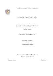
12 1 Historical Background and Physical Motivations1.3 Symmetry, Energy, and EntropyAt this point, let us focus on some connections between three key concepts ofphysics, namely symmetry, energy, and entropy: see Fig. 1.1. According to Plato,symmetry sits in Topos Ouranos (heavens), where sit all branches of mathematics –science of structures –. In contrast, energy and entropy sit in Physis (nature). Energydeals with the possibilities of the system; entropy deals with the probabilities ofthose possibilities. It is fair to say that energy is a quite subtle physical concept.Entropy is based upon the ingredients of energy, and therefore is, epistemologicallyspeaking, one step further. It is most likely because of this feature that entropyemerged, in the history of physics, well after energy. A coin has two faces, andcan therefore fall in two possible manners, head and tail (if we disconsider the veryunlike possibility that it falls on its edge). This is the world of the possibilities forthis simple system. The world of its probabilities is more delicate. Before throwingthe coin (assumed fair for simplicity), the entropy equals ln 2. After throwing it,it still equals ln 2 for whoever has not seen the result (or just does not know it),whereas it equals zero for whoever has seen the outcome (or knows it). This exampleneatly illustrates the informational nature of the concept.Let us now address the connections. Those between symmetry and energy arelong and well known. Galilean invariance of the equations is central to Newtonianmechanics. Its simplest form of energy can be considered to be the kinetic one of apoint particle, namely p 2 /2m, p being the linear momentum, and m the mass. Thisenergy, although having an unique form, is not universal; indeed it depends on themass of the system. If we replace now the Galilean invariance by the Lorentzian one,this drastically changes the form itself of the kinetic energy, which now becomes(p 2 c 2 + m 2 0 c4 ) 1/2 , c being the speed of light in vacuum, and m 0 the mass at rest. InFig. 1.1 Connections between symmetry, energy, and entropy. QED and QCD respectively denotequantum electrodynamics and quantum chromodynamics.

1.4 A Few Words on the Foundations of Statistical Mechanics 13other words, this change of symmetry is far from innocuous; it does nothing less thanchanging Newtonian mechanics into special relativity! Maxwell electromagnetismis, as well known, deeply related to this same Lorentzian invariance, as well as togauge invariance. The latter plays, in turn, a central role in quantum electrodynamicsand quantum field theory. Quantum chromodynamics also is deeply related to symmetryproperties. And so is expected to be quantum gravity, whenever it becomesreality. Summarizing, the deep connections between symmetry and energy are standardknowledge in contemporary physics. Changes in one of them are concomitantlyfollowed by changes in the other one.What about the connections between energy and entropy? Well, also these arequite known. They naturally emerge in thermodynamics (the possibility and mannersfor transforming work into heat, and the other way around). This obviouslyreflects on BG statistical mechanics itself.But, what can we say about the possible connections between symmetry (its natureand evolution) and entropy? This topic has remained basically unchanged andvirtually unexplored during more than one century! Why? Hard to know. However,it is allowed to suspect that this intellectual lethargy comes, on one hand, from the“sloppiness” of the concept of entropy, and, on the other one, from the remarkablefact that the unique functional form that has been used in thermal equilibrium-likephysics is the BG one (Eq. (1.8) and its continuum or quantum analogs), which dependsonly on one of the universal constants, namely Boltzmann constant k B . Withinthis intellectual landscape, generation after generation, the idea installed in the mindof very many physicists that the physical entropy must be universal, and that it is ofcourse the BG one. In the present book, we try to convince the reader that it is notso, that many types of entropy can be physically and mathematically meaningful.Moreover, we shall argue that dynamical concepts such as the time-dependence ofthe sensitivity to the initial conditions, mixing, and the associated occupancy andvisitation networks they may cause in phase-space, have so strong effects, that eventhe functional form of the entropy must, in some occasions, be modified. The BGentropy will then still have a highly priviledged position. It surely is the correct onewhen the microscopic nonlinear dynamics is controlled by positive Lyapunov exponents,hence strong chaos. If the system is such that strong chaos is absent (typicallybecause the maximal Lyapunov exponent vanishes), then the physical entropy to beused appears to be a different one.1.4 A Few Words on the Foundations of Statistical MechanicsA mechanical foundation of statistical mechanics from first principles should essentiallyinclude, in one way or another, the following main steps [40].(i) Adopt a microscopic dynamics. This dynamics typically is deterministic, i.e.,without any phenomenological noise or stochastic ingredient, so that the foundationmay be considered as from first principles. This dynamics could be Newtonian, orquantum, or relativistic mechanics (or some other mechanics to be found in fu-

14 1 Historical Background and Physical Motivationsture) of a many-body system composed by say N interacting elements or fields. Itcould also be conservative or dissipative coupled maps, or even cellular automata.Consistently, time t could be continuous or discrete. The same is valid for space.The quantity which is defined in space-time could itself be continuous or discrete.For example, in quantum mechanics, the quantity is a complex continuous variable(the wave function) defined in a continuous space-time. On the other extreme, wehave cellular automata, for which all three relevant variables – time, space, andthe quantity therein defined – are discrete. In the case of a Newtonian mechanicalsystem of particles, we may think of N Dirac delta functions localized in continuousspatial positions which depend on a continuous time.Langevin-like equations (and associated Fokker-Planck-like equations) are typicallyconsidered not microscopic, but mesoscopic instead. The reason of courseis the fact that they include at their very formulation, i.e., in an essential manner,some sort of (stochastic) noise. Consequently, they should not be used as astarting point if we desire the foundation of statistical mechanics to be from firstprinciples.(ii) Then assume some set of initial conditions and let the system evolve intime. These initial conditions are defined in the so-called phase-space of the microscopicconfigurations of the system, for example Gibbs’ space for a NewtonianN-particle system (the space for point masses has 2dN dimensions if theparticles live in a d-dimensional space). These initial conditions typically (but notnecessarily) involve one or more constants of motion. For example, if the system isa conservative Newtonian one of point masses, the initial total energy and the initialtotal linear momentum (d dimensional vector) are such constants of motion. Thetotal angular momentum might also be a constant of motion. It is quite frequent touse coordinates such that both total linear momentum and total angular momentumvanish.If the system consists of conservative coupled maps, the initial hypervolume of anensemble of initial conditions near a given one is preserved through time evolution.By the way, in physics, such coupled maps are frequently obtained through Poincarésections of Newtonian dynamical systems.(iii) After some sufficiently long evolution time (which typically depends on bothN and the spatial range of the interactions), the system might approach some stationaryor quasi-stationary macroscopic state. 2 In such a state, the various regions ofphase-space are being visited with some probabilities. This set of probabilities eitherdoes not depend anymore on time or depends on it very slowly. More precisely, if itdepends on time, it does so on a scale much longer than the microscopic time scale.The visited regions of phase-space that we are referring to typically correspond to apartition of phase-space with a degree of (coarse or fine) graining that we adopt forspecific purposes. These probabilities can be either insensitive or, on the contrary,very sensitive to the ordering in which t →∞(asymptotic) and N →∞(thermodynamic)limits are taken. This can depend on various aspects such as the range of2 When the system exhibits some sort of aging, the expression quasi-stationary is preferable tostationary.

1.4 A Few Words on the Foundations of Statistical Mechanics 15the interactions, or whether the system is on the ordered or on the disordered sideof a continuous phase transition. Generically speaking, the influence of the orderingof t →∞and N →∞limits is typically related to some kind of breakdown ofsymmetry, or of ergodicity, or the alike.The simplest nontrivial dynamical situation is expected to occur for an isolatedmany-body short-range-interacting classical Hamiltonian system (microcanonicalensemble); later on we shall qualify when an interaction is considered short-rangedin the present context. In such a case, the typical microscopic (nonlinear) dynamicsis expected to be strongly chaotic, in the sense that the maximal Lyapunov exponentis positive. Such a system would necessarily be mixing, i.e., it would quickly visitvirtually all the accessible phase-space (more precisely, very close to almost all theaccessible phase-space) for almost any possible initial condition. Furthermore, itwould necessarily be ergodic with respect to some measure in the full phase-space,i.e., time averages and ensemble averages would coincide. In most of the casesthis measure is expected to be uniform in phase-space, i.e., the hypothesis of equalprobabilities would be satisfied.A slightly more complex situation is encountered for those systems which exhibita continuous phase transition. Let us consider the simple case of a ferromagnetwhich is invariant under inversion of the hard axis of magnetization, e.g., the d = 3XY classical nearest-neighbor ferromagnetic model on simple cubic lattice. If thesystem is in its disordered (paramagnetic) phase, the limits t →∞and N →∞commute, and the entire phase-space is expected to be equally well visited. If thesystem is in its ordered (ferromagnetic) phase, the situation is expected to be moresubtle. The lim N→∞ lim t→∞ set of probabilities is, as before, equally distributed allover the entire phase-space for almost any initial condition. But this is not expectedto be so for the lim t→∞ lim N→∞ set of probabilities. The system probably lives, inthis case, only in half of the entire phase-space. Indeed, if the initial condition is suchthat the initial magnetization is positive, even infinitesimally positive (for instance,under the presence of a vanishingly small external magnetic field), then the systemis expected to be ergodic but only in the half phase-space associated with positivemagnetization; the other way around occurs if the initial magnetization is negative.This illustrates, already in this simple example, the importance that the ordering ofthose two limits can have.A considerably more complex situation is expected to occur, if we consider along-range-interacting model, e.g., the same d = 3 XY classical ferromagneticmodel on simple cubic lattice as before, but now with a coupling constant whichdecays with distance as 1/r α , where r is the distance measured in crystal units,and 0 ≤ α ≤ d (the nearest-neighbor model that we just discussed correspondsto α →∞, which is the extreme case of the short-ranged domain α>d). The0 ≤ α/d ≤ 1 model also appears to have a continuous phase transition. In thedisordered phase, the system possibly is ergodic over the entire phase-space. Butin the ordered phase the result can strongly depend on the ordering of the twolimits. The lim N→∞ lim t→∞ set of probabilities corresponds to the system livingin the entire phase-space. In contrast, the lim t→∞ lim N→∞ set of probabilities forthe same (conveniently scaled) total energy might be considerably more complex. Itseems that, for this ordering, phase-space exhibits at least two macroscopic basins

16 1 Historical Background and Physical Motivationsof attraction. One of them leads essentially to half of the same phase-space wherethe system lives in the lim N→∞ lim t→∞ ordering, i.e., the half phase-space whichis associated with a sign for the magnetization which coincides with the sign of theinitial magnetization. The other basin of attraction could well correspond to living ina very complicated, hierarchical-like, geometrical structure. This structure could bea zero Lebesgue measure one (in the full multidimensional phase-space), somewhatsimilar to that of an airlines company, say Air France, whose central hub is located inParis, or Continental Airlines, whose central hub is located in Houston. The specificlocation of the structure in phase-space would depend on the particular initial conditionwithin that special basin of attraction, but the geometrical–dynamical nature ofthe structure would be virtually the same for any initial condition within that basinof attraction. At this point, let us warn the reader that the scenario that we havedepicted here is only conjectural, and remains to be proved. It is however basedon various numerical evidences (see, e.g., [41, 44, 45, 50] and references therein). Itis expected to be caused by a possibly vanishing maximal Lyapunov exponent. Inother words, one would possibly have, instead of strong, only weak chaos.(iv) Now let us focus further on the specific role played by the initial conditions.If the system is strongly chaotic, hence mixing, hence ergodic, this point isirrelevant. We can make or not averages over initial conditions, we can take almostany initial condition, the outcome for sufficiently long times will be the same, in thesense that the set of probabilities in phase-space will be the same. But if the system isonly weakly chaotic, the result can drastically change from initial condition to initialcondition. If two initial conditions belong to the same “basin of attraction,” the differenceat the macroscopic level could be quite irrelevant. If they belong however todifferent basins of attraction, the results can be sensibly different. For some purposeswe might wish to stick to a specific initial condition within a certain class of initialconditions. For other purposes, we might wish to average over all initial conditionsbelonging to a given basin of attraction, or even over all possible initial conditionsof the entire phase-space. The macroscopic result obtained after averaging mightconsiderably differ from that corresponding to a single initial condition.(v) Last but not least, the mathematical form of the entropy functional must beaddressed. Strictly speaking, if we have deduced (from microscopic dynamics) theprobabilities to be associated with every cell in phase-space, we can in principlecalculate useful averages of any physical quantity of interest which is defined inthat phase-space. In this sense, we do not need to introduce an entropic functionalwhich is defined precisely in terms of those probabilities. Especially if we take intoaccount that any set of physically relevant probabilities can be obtained throughextremization (typically maximization) of an infinite number of entropic functionals(monotonically depending one onto the other), given any set of physically andmathematically meaningful constraints. However, if we wish to make contact withclassical thermodynamics, we certainly need to know the mathematical form of suchentropic functional. This functional is expected to match, in the appropriate limits,the classical, macroscopic, entropy ‘a la Clausius. In particular, one expects it tosatisfy the Clausius property of extensivity, i.e., essentially to be proportional to the

1.4 A Few Words on the Foundations of Statistical Mechanics 17weight or mass of the system. In statistical mechanical terms, we expect it to beproportional to N for large N. 3The foundations of any statistical mechanics are, as already said, expected tocover basically all of the above points. There is a wide-spread vague belief amongphysicists that these steps have already been satisfactorily accomplished since longfor the standard, BG statistical mechanics. This is not so! Not so surprising after all,given the enormity of the corresponding task! For example, as already mentioned, atthis date, there is no available deduction, from and only from microscopic dynamics,of the celebrated BG exponential weight (1.8). Neither exists the deduction frommicroscopic dynamics of the BG entropy (1.1).For standard systems, there is not a single reasonable doubt about the correctnessof the expressions (1.1) and (1.8) and of their relationships. But, from the logicaldeductiveviewpoint, there is still pretty much work to be done! This is, in fact,kind of easy to notice. Indeed, all the textbooks, without exception, introduce theBG factor and/or the entropy S BG in some kind of phenomenological manner, oras self-evident, or within some axiomatic formulation. None of them introducesthem as (and only as) a rational consequence of Newtonian, or quantum mechanics,using theory of probabilities. This is in fact sometimes referred to as the Boltzmannprogram. Boltzmann himself died without succeeding its implementation. Althoughimportant progress has been accomplished in these last 130 years, Boltzmann programstill remains in our days as a basic intellectual challenge. Were it not thegenius of scientists like Boltzmann and Gibbs, were we to exclusively depend onmathematically well-constructed arguments, one of the monuments of contemporaryphysics – BG statistical mechanics – would not exist!Many anomalous natural, artificial, and social systems exist for which BG statisticalconcepts appear to be inapplicable. Typically because they live in peculiarstationary or quasi stationary states that are quite different from thermal equilibrium,where BG statistics reigns. Nevertheless, as we shall see, some of them can still behandled within statistical mechanical methods, but with a more general entropy,namely S q , to be introduced later on [39, 59, 60].It should be clear that, whatever is not yet mathematically justified in BG statisticalmechanics, it is even less justified in the generalization to which the presentbook is dedicated. In addition to this, some of the points that are relatively wellunderstood in the standard theory can be still unclear in its generalization. In otherwords, the theory we are presenting here is still in intense evolution (sets of reviewscan be found in [62, 64–76]).3 Let us anticipate that it has been recently shown [55–58] that, if we impose a Poissonian distributionfor visitation times in phase-space, in addition to the first and second principles of thermodynamics,we obtain the BG functional form for the entropy. If a conveniently deformed Poissoniandistribution is imposed instead, we obtain the S q functional form. These results in themselvescannot be considered as a justification from first principles of the BG, or of the nonextensive, statisticalmechanics. Indeed, the visitation distributions are phenomenologically introduced, and thefirst and second principles are just imposed. This connection is nevertheless extremely clarifying,and can help producing a full justification.

Chapter 2Learning with Boltzmann–Gibbs StatisticalMechanics ˜ ´o ´ , o [78]Kleoboulos of Lindos (6th century B.C.)2.1 Boltzmann–Gibbs Entropy2.1.1 Entropic FormsThe entropic forms (1.1) and (1.3) that we have introduced in Chapter 1 correspondto the case where the (microscopic) states of the system are discrete. There are,however, cases in which the appropriate variables are continuous. For these, the BGentropy takes the form∫S BG =−kdx p(x) ln[σ p(x)] , (2.1)with∫dx p(x) = 1 , (2.2)where x/σ ∈ R D , D ≥ 1 being the dimension of the full space of microscopicstates (called Gibbs phase-space for classical Hamiltonian systems). Typically xcarries physical units. The constant σ carries the same physical units as x, so thatx/σ is a dimensionless quantity (we adopt from now on the notation [x] = [σ ],hence [x/σ ] = 1). For example, if we are dealing with an isolated classical N-bodyHamiltonian system of point masses interacting among them in d dimensions, wemay use σ = Nd . This standard choice comes of course from the fact that, ata sufficiently small scale, Newtonian mechanics becomes incorrect and we mustrely on quantum mechanics. In this case, D = 2dN, where each of the d pairs ofcomponents of momentum and position of each of the N particles has been takenC. Tsallis, Introduction to Nonextensive Statistical Mechanics,DOI 10.1007/978-0-387-85359-8 2, C○ Springer Science+Business Media, LLC 200919

20 2 Learning with Boltzmann–Gibbs Statistical Mechanicsinto account (we recall that [momentum][position] = []). For the case of equalprobabilities (i.e., p(x) = 1/, where is the hypervolume of the admissibleD-dimensional space), we haveS BG = k ln(/σ ) . (2.3)A particular case of p(x) is the following one:p(x) =W∑p i (x − x i ) (W ≡ /σ ) , (2.4)i=1where (x −x i ) denotes a normalized uniform distribution centered on x i and whose“width” is σ (hence its height is 1/σ ). In this case, Eqs. (2.1), (2.2) and (2.3) preciselyrecover Eqs. (1.1), (1.2) and (1.3).In both discrete and continuous cases that we have addressed until now, wewere considering classical systems in the sense that all physical observables arereal quantities and not operators. However, for intrinsically quantum systems, wemust generalize the concept. In that case, the BG entropic form is to be written (asfirst introduced by von Neumann) in the following manner:S BG =−kTrρ ln ρ, (2.5)withTrρ = 1 , (2.6)where ρ is the density matrix acting on a W -dimensional Hilbert vectorial space(typically associated with the solutions of the Schroedinger equation with the chosenboundary conditions; in fact, quite frequently we have W →∞).A particular case of ρ is when it is diagonal, i.e., the following one:ρ ij = p i δ ij , (2.7)where δ ij denotes Kroenecker’s delta function. In this case, Eqs. (2.5) and (2.6)exactly recover Eqs. (1.1) and (1.2).All three entropic forms (1.1), (2.1), and (2.5) will be generically referred in thepresent book as BG-entropy because they are all based on a logarithmic measurefor disorder. Although we shall use one or the other for specific purposes, we shallmainly address the simple form expressed in Eq. (1.1).

2.1 Boltzmann–Gibbs Entropy 212.1.2 Properties2.1.2.1 Non-negativityIf we know with certainty the state of the system, then p i0 = 1, and p i =0, ∀ i ≠ i 0 . Then it follows that S BG = 0, where we have taken into account thatlim x→0 (x ln x) = 0. In any other case, we have p i < 1 for at least two differentvalues of i. We can therefore write Eq. (1.1) as follows:〈S BG =−k〈ln p i 〉=k ln 1 〉,p i(2.8)where 〈···〉 ≡ ∑ Wi=1 p i(...) is the standard mean value. Since ln(1/p i ) > 0(∀i), itclearly follows that S BG is positive.2.1.2.2 Maximal at Equal ProbabilitiesEnergy is a concept which definitively takes into account the physical nature of thesystem. Less so, in some sense, the BG entropy. 1 This entropy depends of courseon the total number of possible microscopic configurations of the system, but it isinsensitive to its specific physical support; it only takes into account the (abstract)probabilistic information on the system. Let us make a trivial illustration: a spinthat can be up or down (with regard to some external magnetic field), a coin thatcomes head or tail, and a computer bit which can be 0 or 1 are all equivalent forthe concept of entropy. Consequently, entropy is expected to be a functional whichis invariant with regard to any permutations of the states. Indeed, expression (1.1)exhibits this invariance through the form of a sum. Consequently, if W > 1, theentropy must have an extremum (maximum or minimum), and this must occur forequal probabilities. Indeed, this is the unique possibility for which the entropy isinvariant with regard to the permutation of any two states. It is easy to verify that itis a maximum, and not a minimum. In fact, the identification as a maximum (andnot a minimum) will become obvious when we shall prove, later on, that S BG is aconcave functional. Of course, the expression that S BG takes for equal probabilitieshas already been indicated in Eq. (1.3).2.1.2.3 ExpansibilityAdding to a system new possible states with zero probability should not modifythe entropy. This is precisely what is satisfied by S BG if we take into account the1 This statement is to be revisited for the more general entropy S q . Indeed, as we shall see, theindex q does depend on some universal aspects of the physical system, e.g., the type of inflexionof a dissipative unimodal map, or, possibly, the type of power-law decay of long-range interactionsfor Hamiltonian systems.

22 2 Learning with Boltzmann–Gibbs Statistical Mechanicsalready-mentioned property lim x→0 (x ln x) = 0. So, we have thatS BG (p 1 , p 2 ,...,p W , 0) = S BG (p 1 , p 2 ,...,p W ) . (2.9)2.1.2.4 AdditivityLet O be a physical quantity associated with a given system, and let A and B betwo probabilistically independent subsystems. We shall use the term additive if andonly if O(A + B) = O(A) + O(B). If so, it is clear that if we have N equal systems,then O(N) = NO(1), where the notation is self-explanatory. A weaker conditionis O(N) ∼ N for N → ∞, with 0 < || < ∞, i.e., lim N→∞ O(N)/N isfinite (generically ≠ O(1)). In this case, the expression asymptotically additivemight be used. Clearly, any observable, which is additive with regard to a givencomposition law, is asymptotically additive (with = O(1)), but the opposite isnot necessarily true.It is straightforwardly verified that, if A and B are independent, i.e., if the jointprobability satisfies p A+Bij= pi A p B j(∀(ij)), thenTherefore, the entropy S BG is additive.S BG (A + B) = S BG (A) + S BG (B) . (2.10)2.1.2.5 ConcavityLet us assume two arbitrary and different probability sets, namely {p i } and {pi ′},associated with a single system having W states. We define an intermediate probabilityset as follows:p ′′i = λp i + (1 − λ)p ′ i (∀i; 0 0) satisfies−p i ′′ ln p i ′′ >λ(−p i ln p i ) + (1 − λ)(−p i ′ ln p′ i ) (∀i; 0

2.1 Boltzmann–Gibbs Entropy 232.1.2.6 Lesche-Stability or Experimental RobustnessAn entropic form S({p i }) (or any other functional of the probabilities, in fact) is saidLesche-stable or experimentally robust [79] if and only if it satisfies the followingcontinuity property. Two probability distributions {p i } and {pi ′ } are said close if theysatisfy the metric property:D ≡W∑|p i − p i ′ |≤d ɛ , (2.14)i=1where d ɛ is a small real number. Then, experimental robustness is verified if, for anyɛ>0, a d ɛ exists such that D ≤ d ɛ impliesR ≡∣ S({p i}) − S({p ′ i })S max∣ ∣∣ 0) . (2.17)Equation (2.14) corresponds to μ = 1. The Pythagorean metric corresponds toμ = 2. What about other values of μ? It happens that only for μ ≥ 1 the triangularinequality is satisfied, and consequently it does constitute a metric. Still, why not

24 2 Learning with Boltzmann–Gibbs Statistical Mechanics0R BG-0.2-0.4-0.6d = 0.1d = 0.001d = 0.01-0.8-1QC0 0.1 0.2 0.3 0.4 0.51/W0.1R BG d = 0.10d = 0.001-0.1d = 0.01-0.2-0.3QEP0 0.1 0.2 0.3 0.4 0.51/WFig. 2.1 Illustration of the Lesche-stability of S BG . QC and QEP stand for quasi-certainty andquasi-equal-probabilities, respectively (see details in [110, 113]).using values of μ>1? Because, only for μ = 1, the distance D does not dependon W , which makes it appropriate for a generic property [80].We come back in Section 3.2.2 onto this interesting property introduced byLesche.2.1.2.7 Shannon Uniqueness TheoremLet us assume that an entropic form S({p i }) satisfies the following properties:(i) S({p i }) is a continuous f unction of {p i }; (2.18)(ii) S(p i = 1/W, ∀i) monotonically increases with the totalnumber of possibilities W; (2.19)(iii) S(A + B) = S(A) + S(B) if p A+Bij= pi A p B j ∀(i, j) , (2.20)

2.1 Boltzmann–Gibbs Entropy 25where S(A + B) ≡ S({p A+Bij}), S(A) ≡ S({pi A })(piA ≡and S(B) ≡ S({p B j })(pB j ≡∑W Ai=1p A+Bij);∑W Bj=1p A+Bij) ,(iv) S({p i }) = S(p L , p M ) + p L S({p i /p L }) + p M S({p i /p M }) (2.21)with p L ≡ ∑p i , p M ≡∑p i ,LtermsL + M = W , and p L + p M = 1 .Then and only then [25]S({p i }) =−kMtermsW∑p i ln p i (k > 0) . (2.22)i=12.1.2.8 Khinchin Uniqueness TheoremLet us assume that an entropic form S({p i }) satisfies the following properties:(i) S({p i }) is a continuous f unction of {p i }; (2.23)(ii) S(p i = 1/W, ∀i) monotonically increases with the totalnumber of possibilities W; (2.24)(iii) S(p 1 , p 2 ,...,p W , 0) = S(p 1 , p 2 ,...,p W ); (2.25)(iv) S(A + B) = S(A) + S(B|A), (2.26)where S(A + B) ≡ S({p A+Bij}), S(A) ≡ S({pi A })(piA ≡and the conditional entropy S(B|A) ≡Then and only then [81]2.1.2.9 ComposabilityS({p i }) =−k∑W Api A S({p A+Biji=1∑W Bj=1p A+Bij) ,/p Ai }) .W∑p i ln p i (k > 0) . (2.27)i=1A dimensionless entropic form S({p i }) (i.e., whenever expressed in appropriate conventionalunits, e.g., in units of k) issaidcomposable if the entropy S(A + B)corresponding to a system composed of two independent subsystems A and B canbe expressed in the form

26 2 Learning with Boltzmann–Gibbs Statistical MechanicsS(A + B) = F(S(A), S(B); {η}) , (2.28)where F(x, y; {η}) is a function which, besides depending symmetrically on (x, y),depends on a (typically small) set of universal indices {η}. In other words, it doesnot depend on the microscopic configurations of A and B. Equivalently, we are ableto macroscopically calculate the entropy of the composed system without any needof entering into the knowledge of the microscopic states of the subsystems. Thisproperty appears to be a natural one for an entropic form if we desire to use it as abasis for a statistical mechanics which would naturally connect to thermodynamics.The BG entropy is composable since it satisfies Eq. (2.10). In other words, wehave F(x, y) = x + y. Since S BG is nonparametric, no index exists.2.1.2.10 Sensitivity to the Initial Conditions, Entropy Production per UnitTime, and a Pesin-Like IdentityFor a one-dimensional dynamical system (characterized by the variable x) the sensitivityto the initial conditions ξ is defined as follows:ξ ≡x(t)limx(0)→0 x(0) . (2.29)It can be shown [82, 83] that ξ paradigmatically satisfies the equationwhose solution is given bydξdt= λ 1 ξ, (2.30)ξ = e λ 1 t . (2.31)(The meaning of the subscript 1 will become transparent later on). If the Lyapunovexponent λ 1 > 0(λ 1 < 0), the system will be said to be strongly chaotic (regular).The case where λ 1 = 0 is sometimes called marginal and will be extensivelyaddressed later on.At this point let us briefly review, without proof, some basic notions of nonlineardynamical systems. If the system is d-dimensional (i.e., it evolves in a phase-spacewhose d-dimensional Lebesgue measure is finite), it has d Lyapunov exponents: d +of them are positive, d − are negative, and d 0 vanish, hence d + + d − + d 0 = d. Letus order them all from the largest to the smallest: λ (1)1≥ λ (2)1≥ ... ≥ λ (d +)1>λ (d ++1)1= λ (d ++2)1= ... = λ (d ++d 0 )1= 0 >λ (d ++d 0 +1)1≥ λ (d ++d 0 +2)1≥ ... ≥ λ (d)1 .An infinitely small segment (having then a well defined one-dimensional Lebesguemeasure) diverges like e λ(1) 1 t ; this precisely is the case focused in Eq. (2.31). An infinitelysmall area (having then a well defined two-dimensional Lebesgue measure)diverges like e (λ(1) 1 +λ(2) 1 ) t . An infinitely small volume diverges like e (λ(1) 1 +λ(2) 1 +λ(3) 1 ) t , andso on. An infinitely small d-dimensional hypervolume evolves like e [∑ dr=1 λ(r) 1 ] t .If

2.1 Boltzmann–Gibbs Entropy 27the system is conservative, i.e., if the infinitely small d-dimensional hypervolumeremains constant with time, then it follows that ∑ dr=1 λ(r) 1= 0. An important particularclass of conservative systems is constituted by the so-called symplectic ones.For these, d is an even integer, and the Lyapunov exponents are coupled two bytwo as follows: λ (1)1=−λ (d)1≥ λ (2)1=−λ (d−1)1≥ ... ≥ λ (d +)1=−λ (d ++d 0 +1)1≥λ (d ++1)1= ... = λ (d ++d 0 )1= 0. Consistently, such systems have d + = d − andd 0 is an even integer. The most popular illustration of symplectic systems is theHamiltonian systems. They are conservative, which precisely is what the classicalLiouville theorem states!Do all these degrees of freedom contribute, as time evolves, to the erratic explorationof the phase-space? No, they do not. Only those associated with the d + positiveLyapunov exponents, and some of the d 0 vanishing ones, do. Consistently, it isonly these which contribute to our loss of information, as time evolves, about the locationin phase-space of a set of initial conditions. As we shall see, these remarks enablean intuitive understanding to the so-called Pesin identity, that we will soon state.Let us now address the interesting question of the BG entropy production astime t increases. More than one entropy production can be defined as a function oftime. Two basic choices are the so-called Kolmogorov–Sinai entropy (or KS entropyrate) [84], based on a single trajectory in phase-space, and the one associated to theevolution of an ensemble of initial conditions. We shall preferentially use here thelatter, because of its sensibly higher computational tractability. In fact, excepting forpathological cases, they both coincide.Let us schematically describe the Kolmogorov–Sinai entropy rate concept ormetric entropy [83, 84, 286]. We first partition the phase-space in two regions,noted A and B. Then we choose a generic initial condition (the final result willnot depend on this choice) and, applying the specific dynamics of the system atequal and finite time intervals τ, we generate a long string (infinitely long in principle),say ABBBAABBABAAA.... Then we analyze words of length l = 1.In our case, there are only two such words, namely A and B. The analysis consistsin running along the string a window whose width is l, and determiningthe probabilities p A and p B of the words A and B, respectively. Finally, we calculatethe entropy S BG (l = 1) = −p A ln p A − p B ln p B . Then we repeat forwords whose length equals l = 2. In our case, there are four such words, namelyAA, AB, BA, BB. Running along the string a l = 2 window letter by letter,we determine the probabilities p AA , p AB , p BA , p BB , hence the entropy S BG (l =2) =−p AA ln p AA − p AB ln p AB − p BA ln p BA − p BB ln p BB . Then we repeat forl = 3, 4,... and calculate the corresponding values for S BG (l). We then chooseanother two-partition, say A ′ and B ′ , and repeat the whole procedure. Then we doin principle for all possible two partitions. Then we go to three partitions, i.e., thealphabet will be now constituted by three letters, say A, B, and C. We repeat theprevious procedure for l = 1 (corresponding to the words A, B, C), then for l = 2(corresponding to the words AA, AB, AC, BA, BB, BC, CA, CB, CC), etc. Thenwe run windows with l = 3, 4,.... We then consider a different three-partition, sayA ′ , B ′ , and C ′ ...Then we consider four-partitions, and so on. Of all these entropieswe retain the supremum. In the appropriate limits of infinitely fine partitions and

28 2 Learning with Boltzmann–Gibbs Statistical Mechanicsτ → 0 we obtain finally the largest rate of increase of the BG entropy. This isbasically the Kolmogorov–Sinai entropy rate.It is not necessary to insist on how deeply inconvenient this definition can be forany computational implementation! Fortunately, a different type of entropy productioncan be defined [85], whose computational implementation is usually very simple.It is defined as follows. First partition the phase-space into W little cells (normallyequal in size) and denote them with i = 1, 2,...,W . Then randomly placeM initial conditions in one of those W cells (if d + ≥ 1, normally the result will notdepend on this choice). And then follow, as time evolves, the number of points M i (t)in each cell ( ∑ Wi=1 M i(t) = M). Define the probability set p i (t) ≡ M i (t)/M (∀i),and calculate finally S BG (t) through Eq. (1.1). The entropy production per unit timeis defined asK 1 ≡ limlimlimt→∞ W →∞ M→∞S BG (t)t. (2.32)The Pesin identity [86], or more precisely the Pesin-like identity that we shalluse here, states, for large classes of dynamical systems [85],K 1 =d +∑r=1λ (r)1 . (2.33)As it will become gradually clear along the book, this relationship (and its q-generalization) will play an important role in the determination of the particularentropic form which is adequate for a given nonlinear dynamical system.2.2 Kullback–Leibler Relative EntropyIn many problems the question arises on how different are two probability distributionsp and p (0) ; for reasons that will become clear soon, p (0) will be referred toas the reference. It becomes therefore interesting to define some sort of “distance”between them. One possibility is of course the distance introduced in Eq. (2.17). Inother words, for say continuous distributions, we can use[ ∫D μ (p, p (0) ) ≡ dx |p(x) − p (0) (x)| μ] 1/μ(μ >0) . (2.34)In general we have that D μ (p, p (0) ) = D μ (p (0) , p), and that D μ (p, p (0) ) = 0if and only if p(x) = p (0) (x) almost everywhere. We remind, however, that thetriangular inequality is satisfied only for μ ≥ 1. Therefore, only then the distanceconstitutes a metric. If p(x) = ∑ Wi=1 p i (x −x i ) and p (0) (x) = ∑ Wi=1 p(0) i(x −x i ),(see Eq. (2.4)) Eq. (2.34) leads to

2.2 Kullback–Leibler Relative Entropy 29[ ∑WD μ (p, p (0) ) ≡ |p i − p (0)i| μ] 1/μi=1(μ >0) , (2.35)which exactly recovers Eq. (2.17).For some purposes, this definition of distance is quite convenient. For others, theKullback–Leibler entropy [87] has been introduced (see, for instance, [88, 92] andreferences therein). It is occasionally called cross entropy, orrelative entropy, ormutual information, and it is defined as follows:∫I 1 (p, p (0) ) ≡[ p(x)] ∫dx p(x)ln =−p (0) (x)[ p (0) (x)dx p(x)lnp(x)]. (2.36)It can be proved, by using ln r ≥ 1 − 1/r (with r ≡ p(x)/p (0) (x) > 0),that I 1 (p, p (0) ) ≥ 0, the equality being valid if and only if p(x) = p (0) (x) almosteverywhere. It is clear that in general I 1 (p, p (0) ) ≠ I 1 (p (0) , p). This inconvenienceis sometimes overcome by using the symmetrized quantity [I 1 (p, p (0) ) +I 1 (p (0) , p)]/2.I 1 (p, p (0) ) (like the distance (2.34)) has the property of being invariant undervariable transformation. Indeed, if we make x = f (y), the measure preservationimplies p(x)dx = ˜p(y)dy. Since p(x)/p (0) (x) = ˜p(x)/ ˜p (0) (x), we haveI 1 (p, p (0) ) = I 1 ( ˜p, ˜p (0) ), which proves the above-mentioned invariance. The BGentropy in its continuous (not in its discrete) form S BG =− ∫ dx p(x)lnp(x) lacksthis important property. Because of this fact, the BG entropy is advantageouslyreplaced, in some calculations, by the Kullback–Leibler one. Depending on theparticular problem, the referential distribution p (0) (x) is frequently taken to be astandard distribution such as the uniform, or Gaussian, or Lorentzian, or Poissonor BG ones. When p (0) (x) is chosen to be the uniform distribution on a compactsupport of Lebesgue measure W , we have the relationI 1 (p, 1/W ) = ln W − S BG (p) . (2.37)Because of relations of this kind, the minimization of the Kulback–Leibler entropyis sometimes used instead of the maximization of the Boltzmann–Gibbs–Shannon entropy.Although convenient for a variety of purposes, I 1 (p, p (0) ) has a disadvantage.It is needed that p(x) and p (0) (x) simultaneously vanish, if they do so for certainvalues of x (this property is usually referred to as being absolutely continuous).Indeed, it is evident that otherwise the quantity I 1 (p, p (0) ) becomes ill-defined. Toovercome this difficulty, a different distance has been defined along the lines of theKullback–Leibler entropy. We refer to the so-called Jensen–Shannon divergence.Although interesting in many respects, its study would take us too far from ourpresent line. Details can be seen in [93, 94] and references therein.

30 2 Learning with Boltzmann–Gibbs Statistical MechanicsLet us mention also that, for discrete probabilities, definition (2.36) leads toI 1 (p, p (0) ) ≡W∑i=1[ pi]p i lnp (0) =−iW∑i=1[ p(0) ]ip i ln . (2.38)p iVarious other interesting related properties can be found in [95, 96].2.3 Constraints and Entropy OptimizationThe most simple entropic optimization cases are those worked out in what follows.2.3.1 Imposing the Mean Value of the VariableIn addition to∫ ∞we might know the mean value of the variable, i.e.,〈x〉 ≡0∫ ∞0dx p(x) = 1 , (2.39)dx xp(x) = X (1) . (2.40)By using the Lagrange method to find the optimizing distribution, we define[p] ≡−∫ ∞0dx p(x)lnp(x) − α∫ ∞0∫ ∞dx p(x) − β (1) dx xp(x) , (2.41)and then impose δ[p]/δp(x) = 0. We straightforwardly obtain 1 + ln p opt + α +β (1) x = 0(opt stands for optimal), hencep opt =e −β(1) x∫ ∞0dx e −β(1) x = β(1) e −β(1)x , (2.42)where we have used condition (2.39) to eliminate the Lagrange parameter α. Byusing condition (2.40), we obtain the following relation for the Lagrange parameterβ (1) :hence, replacing in (2.42),β (1) = 1 , (2.43)X(1)0

2.3 Constraints and Entropy Optimization 31p opt =e−x/ X (1)X (1) . (2.44)2.3.2 Imposing the Mean Value of the Squared VariableAnother simple and quite frequent case is when we know that 〈x〉 =0. In such case,in addition to∫ ∞−∞we might know the mean value of the squared variable, i.e.,〈x 2 〉≡∫ ∞−∞dx p(x) = 1 , (2.45)dx x 2 p(x) = X (2) > 0 . (2.46)By using, as before, the Lagrange method to find the optimizing distribution, wedefine∫ ∞∫ ∞∫ ∞[p] ≡− dx p(x)lnp(x) − α dx p(x) − β (2) dx x 2 p(x) , (2.47)−∞−∞−∞and then impose δ[p]/δp(x) = 0. We straightforwardly obtain 1 + ln p opt + α +β (2) x 2 = 0, hencep opt =e −β(2) x 2∫ ∞−∞ dx e−β(2) x 2 = √β(2)π e−β(2) x 2 , (2.48)where we have used condition (2.45) to eliminate the Lagrange parameter α.By using condition (2.46), we obtain the following relation for the Lagrangeparameter β (2) :hence, replacing in (2.48),β (2) = 1 , (2.49)2X(2)p opt = e− x2 /(2X (2) )√2π X(2). (2.50)We thus see the very basic connection between Gaussian distributions and BGentropy.

32 2 Learning with Boltzmann–Gibbs Statistical Mechanics2.3.3 Imposing the Mean Values of both the Variableand Its SquareLet us unify here the two preceding subsections. We impose∫ ∞−∞and, in addition to this, we know thatdx p(x) = 1 (2.51)〈x〉 ≡and〈(x −〈x〉) 2 〉≡∫ ∞−∞∫ ∞−∞dx xp(x) = X (1) , (2.52)dx (x −〈x〉) 2 p(x) = X (2) − (X (1) ) 2 ≡ M (2) > 0 . (2.53)By using once again the Lagrange method, we define∫ ∞∫ ∞[p] ≡− dx p(x)lnp(x) − α dx p(x)−∞−∞∫ ∞∫ ∞−β (1) dx x p(x) − β (2) dx (x −〈x〉) 2 p(x) , (2.54)−∞and then impose δ[p]/δp(x) = 0. We straightforwardly obtain 1 + ln p opt + α +β (1) x + β (2) (x −〈x〉) 2 = 0, hence−∞p opt =√e −β(1) x−β (2) (x−〈x〉) 2β(2)(x−〈x〉)∫ ∞−∞ dx =2e−β(1) x−β (2) (x−〈x〉) 2 π e−β(2) , (2.55)where we have used condition (2.51) to eliminate the Lagrange parameter α.Byusingconditions (2.52) and (2.53), we obtain the following relations for the Lagrangeparameters β (1) and β (2) :andβ (2) =β (1) = 1 , (2.56)X(1)12[X (2) − (X (1) ) 2 ] . (2.57)

2.4 Boltzmann–Gibbs Statistical Mechanics and Thermodynamics 33Replacing (2.57) in (2.55), we finally obtainp opt =e − (x−X (1) ) 22[X (2) −(X (1) ) 2 ]√2π[X(2)− (X (1) ) 2 ] . (2.58)We see that the only effect of a nonzero mean value of x is to re-center theGaussian.2.3.4 OthersA quite general situation would be to impose, in addition to∫dx p(x) = 1 , (2.59)the constraint∫dx f(x) p(x) = F , (2.60)where f (x) is some known function and F a known number. We obtainp opt =f (x)e−β∫ . (2.61)dx e−β f (x)It is clear that, by appropriately choosing f (x), we can force p opt (x) to be virtuallyany distribution we wish. For example, by choosing f (x) =|x| γ (γ ∈ R), weobtain a generic stretched exponential p opt (x) ∝ e −β|x|γ ; by choosing f (x) = ln x,we obtain for p opt (x) a power law. But the use of such procedures hardly has anyepistemological interest at all, since it provides no hint onto the underlying natureof the problem. Only choices such as f (x) = x or f (x) = x 2 are sound since suchconstraints correspond to very generic informational features, namely the locationof the center and the width of the distribution. Other choices are, unless some exceptionalfact enters into consideration (e.g., f (x) being a constant of motion of thesystem), quite ad hoc and uninteresting. Of course, this mathematical fact is by nomeans exclusive of S BG : the same holds for virtually any entropic form.2.4 Boltzmann–Gibbs StatisticalMechanics and ThermodynamicsThere are many formal manners for deriving the BG entropy and its associatedprobability distribution for thermal equilibrium. None of them uses exclusively firstprinciple arguments, i.e., arguments that entirely remain at the level of mechanics

34 2 Learning with Boltzmann–Gibbs Statistical Mechanics(classical, quantum, relativistic, or any other). That surely was, as previously mentioned,one of the central scientific goals that Boltzmann pursued his entire life,but, although he probably had a strong intuition about this point, he died withoutsucceeding. The difficulties are so heavy that even today we do not know how todo this. At first sight, this might seem surprising given the fact that S BG and theBG weight enjoy the universal acceptance that we all know. So, let us illustrateour statement more precisely. Assume that we have a quite generic many-bodyshort-range-interacting Hamiltonian. We currently know that its thermal equilibriumis described by the BG weight. What we still do not know is how to derive thisimportant result from purely mechanical and statistical logical steps, i.e., withoutusing a priori generic dynamical hypothesis such as ergodicity, or a priori postulatingthe validity of macroscopic relations such as some or all of the principlesof thermodynamics. For example, Fisher et al. [97–99] proved long ago, for a vastclass of short-range-interacting Hamiltonians, that the thermal equilibrium physicalquantities are computable within standard BG statistical mechanics. Such a proof,no matter how precious might it be, does not prove also that this statistics indeedprovides the correct description at thermal equilibrium. Rephrasing, it proves thatBG statistics can be the correct one, but it does not prove that it is the correct one.Clearly, there is no reasonable doubt today that, for such systems, BG is the correctone. It is nevertheless instructive that the logical implications of the available proofsbe outlined.On a similar vein, even for the case of long-range-interacting Hamiltonians (e.g.,infinitely-long-range interactions), the standard BG calculations can still be performedthrough convenient renormalizations of the coupling constants (e.g., alaKac, or through the usual mean field approximation recipe of artificially dividing thecoupling constant by the number N of particles raised to some appropriate power).The possibility of computability does by no means prove, strictly speaking, that BGstatistics is the correct description. And certainly it does not enlighten us on what thenecessary and sufficient first-principle conditions could be for the BG descriptionto be the adequate one.In spite of all these mathematical difficulties, at least one nontrivial examplehas been advanced in the literature [100] for which it has been possible to exhibitnumerically the BG weight by exclusively using Newton’s F = ma as microscopicdynamics, with no thermostatistical assumption of any kind.Let us anticipate that these and worse difficulties exist for the considerably moresubtle situations that will be addressed in nonextensive statistical mechanics.In what follows, we shall conform to more traditional, though epistemologicallyless ambitious, paths. We shall primarily follow the Gibbs’ elegant lines of firstpostulating an entropic form, and then using it, without proof, as the basis for avariational principle including appropriate constraints. The philosophy of such pathis quite clear. It is a form of Occam’ s razor, where we use all that we know andnot more than we know. This is obviously extremely attractive from a conceptualstandpoint. However, that its mathematical implementation is to be done with agiven specific entropic functional with given specific constraints is of course farfrom trivial! After 130 years of impressive success, there can be no doubt that BG

2.4 Boltzmann–Gibbs Statistical Mechanics and Thermodynamics 35concepts and statistical mechanics provide the correct connection between microscopicand macroscopic laws for a vast class of physical systems. But – we insist –the mathematically precise qualification of this class remains an open question.2.4.1 Isolated System – Microcanonical EnsembleIn this and subsequent subsections, we briefly review BG statistical mechanics (see,for instance, [35]). We consider a quantum Hamiltonian system constituted by N interactingparticles under specific boundary conditions, and denote by {E i } its energyeigenvalues.The microcanonical ensemble corresponds to an isolated N-particle systemwhose total energy U is known within some precision δU (tobeinfacttakenatits zero limit at the appropriate mathematical stage). The number of states i withU ≤ E i ≤ U + δU is denoted by W . Assuming that the system is such that itsdynamics leads to ergodicity at its stationary state (thermal equilibrium), we assumethat all such states are equally probable, i.e., p i = 1/W , and the entropy is given byEq. (1.3). The temperature T is introduced through1T ≡ S BGU= k ln WU . (2.62)2.4.2 In the Presence of a Thermostat – Canonical EnsembleThe canonical ensemble corresponds to an N-particle system defined in a Hilbertspace whose dimension is noted W , and which is in longstanding thermal contactwith a (infinitely large) thermostat at temperature T . Its exact energy is unknown,but its mean energy U is known since it is determined by the thermostat. We mustoptimize the entropy given by Eq. (1.1) with the norm constraint (1.2), and with theenergy constraintW∑p i E i = U . (2.63)i=1Following along the lines of Section 2.3, we obtain the celebrated BG weightwith the partition function given byp i = e−β E iZ BG, (2.64)Z BG ≡W∑e −β E i, (2.65)i=1the Lagrange parameter β being related with the temperature through β ≡ 1/(kT).

36 2 Learning with Boltzmann–Gibbs Statistical MechanicsWe can prove also thatthat the Helmholtz free energy is given by1T = S BGU , (2.66)F BG ≡ U − TS BG =− 1 β ln Z BG , (2.67)and that the internal energy is given byU =− β ln Z BG . (2.68)In the limit T →∞we recover the microcanonical ensemble.2.4.3 OthersThe system may be exchanging with the thermostat not only energy, so that thetemperature is that of the thermostat, but also particles, so that also the chemicalpotential is fixed by the reservoir. This physical situation corresponds to the socalledgrand-canonical ensemble. This and other similar physical situations can betreated along the same path, as shown by Gibbs. We shall not review here thesetypes of systems, which are described in detail in [35], for instance.Another important physical case, which we do not review here either, is when theparticles cannot be considered as distinguishable. Such is the case of bosons (leadingto Bose–Einstein statistics), fermions (leading to Fermi–Dirac statistics), and the socalledgentilions (leading to Gentile statistics, also called parastatistics [101–103],which unifies those of Bose–Einstein and Fermi–Dirac).All these various physical systems, and even others, constitute what is currentlyreferred to as BG statistical mechanics, essentially because at its basis we find, inone way or another, the entropic functional S BG . It is this entire theoretical bodythat in principle we intend to generalize in the rest of the book, through the generalizationof S BG itself.

Chapter 3Generalizing What We Learnt: NonextensiveStatistical MechanicsDon Quijote me ha revelado íntimos secretos suyos que noreveló a CervantesVíctor Goti(Prólogo de Niebla de Miguel de Unamuno, 1935)3.1 Playing with Differential Equations – A MetaphorAs we already emphasized, there is no logical-deductive procedure for generalizingany physical theory. This occurs through all types of paths that, in one way or another,are ultimately but metaphors. Let us present here a possible metaphor forgeneralizing the BG entropy.The simplest ordinary differential equation can be considered to beIts solution isdydxwhose symmetric curve with regard to the bissector axis is= 0 (y(0) = 1) . (3.1)y = 1 , (3.2)x = 1 . (3.3)As the second simplest differential equation we might considerIts solution isdydx= 1 (y(0) = 1) . (3.4)y = 1 + x , (3.5)C. Tsallis, Introduction to Nonextensive Statistical Mechanics,DOI 10.1007/978-0-387-85359-8 3, C○ Springer Science+Business Media, LLC 200937

38 3 Generalizing What We Learntwhose inverse function isWe may next wish to consider the following one:whose solution isIts inverse function isand satisfies of coursedydxy = x − 1 . (3.6)= y (y(0) = 1) , (3.7)y = e x . (3.8)y = ln x , (3.9)ln(x A x B ) = ln x A + ln x B . (3.10)Is it possible to unify the three differential equations we considered up to now (i.e.,(3.1), (3.4), and (3.7))? Yes indeed. It is enough to considerdydx= a + by (y(0) = 1) , (3.11)and play with the two parameters a and b. Is it possible to unify the same threedifferential equations with only one parameter? Yes indeed, ...out of linearity!JustconsiderIts solution isIts inverse isdydx = yq (y(0) = 1; q ∈ R) . (3.12)y = [1 + (1 − q)x] 1/(1−q) ≡ e x q (e x 1 = ex ) . (3.13)y = x 1−q − 11 − qand satisfies the following property:≡ ln q x (x > 0; ln 1 x = ln x) , (3.14)ln q (x A x B ) = ln q x A + ln q x B + (1 − q)(ln q x A )(ln q x B ) . (3.15)

3.1 Playing with Differential Equations – A Metaphor 39e qxq = 2 q = 12.5q = 0q → ∞21.51q = –10.5q → –∞–1.5 –1 –0.5 0 0.5 1 x 1.5Fig. 3.1 The q-exponential function eq x for typical values of q. Forq > 1, it is defined in theinterval (−∞, (q − 1) −1 ); it diverges if x → (q − 1) −1 − 0. For q < 1, it is defined ∀x, andvanishes for all x < −(1 − q) −1 . In the limit x → 0, it is eq x ∼ 1 + x (∀q).1e –x q0.80.60.40.2q = –1q = 0q = 2q = 100 1 2 3 x 4Fig. 3.2 The q-exponential function eq−x for typical values of q: linear–linear scales. For q > 1, itvanishes like [(q − 1)x] −1/(q−1) for x →∞.Forq < 1, it vanishes for x > (1 − q) −1 (cutoff).

40 3 Generalizing What We Learnt1e q–xq = 20.1q = 10.01q = –1q = 00 1 2 3 x 4Fig. 3.3 The q-exponential function eq−x for typical values of q: log–linear scales. It is convex(concave) if q > 1(q < 1). For q < 1, it has a vertical asymptote at x = (1 − q) −1 .0.01 0.1 1 10 x 1001e –x q0.1q = 20.01q = –1q = 0 q = 1Fig. 3.4 The q-exponential function eq−x for typical values of q: log–log scales. For q > 1, it hasan asymptotic slope equal to −1/(q − 1).

3.2 Nonadditive Entropy S q 41We shall from now on refer to these two functions as the q-exponential and theq-logarithm, respectively [104]. They will play an important role through the entiretheory. We may, in fact, anticipate that virtually all the generic expressions associatedwith BG statistics and its (nonlinear) dynamical foundations will, remarkablyenough, turn out to be generalized essentially just by replacing the standard exponentialand logarithm forms by the above q-generalized ones. Let us add that,whenever the 1 + (1 − q)x argument of the q-exponential is negative, the functionis defined to vanish. In other words, the definition is eqx ≡ [1 + (1 − q)x]1/(1−q) + ,where [z] + = max{z, 0}. However, for simplicity, we shall, most of the time, avoidthis notation. Typical representations of the q-exponential function are illustrated inFigs. 3.1, 3.2, 3.3, and 3.4. It is immediately verified that the q →−∞, q = 0, andq = 1 particular instances precisely recover the cases presented in Eqs. (3.1), (3.4),and (3.7) respectively.3.2 Nonadditive Entropy S q3.2.1 DefinitionThrough the metaphor presented above, and because of various other reasons thatwill gradually emerge, we may postulate the following generalization of Eq. (1.3):S q = k ln q W (S 1 = S BG ) . (3.16)See Fig. 3.5 for the illustration of this generalization of the celebrated formulafor equal probabilities. Let us address next the general case, i.e., for arbitrary {p i }.We saw in Eq. (2.8) that S BG can be written as the mean value of ln(1/p i ). Thisquantity is called surprise [105] or unexpectedness [106] by some authors. This isquite appropriate, in fact. If we have certainty (p i = 1forsomevalueofi) thatsomething will happen, when it does happen we have no surprise. On the oppositeextreme, if something is very unexpected (p i ≃ 0), if it eventually happens, weare certainly very surprised! Along this line, it is certainly admissible to considerthe quantity ln q (1/p i ) and call it q-surprise or q-unexpectedness. It then appears asquite natural to postulate the simultaneous generalization of Eqs. (2.8) and (3.16) asfollows:S q = k 〈ln q (1/p i )〉 . (3.17)If we use the definition (3.14) in this expression, we straightforwardly obtainS q = k 1 − ∑ Wi=1 pq iq − 1. (3.18)

42 3 Generalizing What We Learnt3q = –1q = 0S q2q = 11q = 201 2 3 4 w 5Fig. 3.5 The equiprobability entropy S q as a function of the number of states W (with k = 1),for typical values of q. Forq > 1, S q saturates at the value 1/(q − 1) if W →∞;forq ≤ 1, itdiverges. For q →∞(q →−∞), it coincides with the abscissa (ordinate).This is precisely the form postulated in [39] as a possible basis for generalizingBG statistical mechanics. See Table 3.1. One possible manner for checking thatS 1 ≡ lim q→1 S q = S BG is to directly replace into Eq. (3.18) the equivalence p q i=p i p q−1i= p i e (q−1) ln p i∼ p i [1 + (q − 1) ln p i ].It turned out that this generalized entropic form, first with a different and thenwith the same multiplying factor, had already appeared outside the literature ofphysics, namely in that of cybernetics and control theory [107]. It was rediscoveredindependently in [39], when it was for the first time proposed as a starting point togeneralize the standard statistical mechanics itself. This was done for the canonicalensemble, by optimizing S q in the presence of an additional constraint, namely thatrelated to the mean value of the energy. We shall focus on this calculation later on.Table 3.1 S BG and S q entropies (S 1 = S BG )Entropy Equal probabilities Generic probabilities(p i = 1/W , ∀i) (∀{p i })S BG k ln W −k ∑ Wi=1 p i ln 2−q p i = k ∑ Wi=1 p i ln(1/p i )S q k ln q W k 1−∑ Wi=1 pq iq−1= k ∑ Wi=1 p i ln q (1/p i )(q ∈ R) =−k ∑ Wi=1 pq iln q p i=−k ∑ Wi=1 p i ln 2−q p i

3.2 Nonadditive Entropy S q 43This form turns out to be in fact directly related to a generalized metric proposedin 1952 by Hardy, Littlewood and Polya [109], whose q = 2 particular case correspondsto the Pythagorean metric.A different path for arriving to the entropy (3.18) is the following one. This wasin fact the original path, inspired by multifractals, that led to the postulate adoptedin [39]. The entropic index q introduces a bias in the probabilities. Indeed, giventhe fact that generically 0 < p i < 1, we have that p q i> p i if q < 1 and p q i< p iif q > 1. Therefore, q < 1 (relatively) enhances the rare events, those which haveprobabilities close to zero, whereas q > 1 (relatively) enhances the frequent events,those whose probability is close to unity. This property can be directly checked ifwe compare p i with p q i / ∑ Wj=1 pq j.So, it appears as appealing to introduce an entropic form based on p q i. We wantalso the form to be invariant under permutations. So the simplest assumption is toconsider S q = f ( ∑ Wi=1 pq i), where f is some continuous function to be found. Thesimplest choice is the linear one, i.e., S q = a+b ∑ Wi=1 pq i. Since any entropy shouldbe a measure of disorder or ignorance, we want that certainty corresponds to zeroentropy. This immediately imposes a + b = 0, hence S q = a(1 − ∑ Wi=1 pq i). But,since we are seeking for a generalization (and not an alternative), for q = 1wewantto recover S BG . Therefore, in the q → 1 limit, a must be asymptotically proportionalto 1/(q − 1) (we remind the equivalence indicated in the previous paragraph). Thesimplest way for this to occur is just to be a = k/(q − 1), with k > 0, whichimmediately leads to Eq. (3.18).We shall next address the properties of S q . But before doing that, let us clarify apoint which has a generic relevance. If q > 0, then expression (3.18) is well definedwhether or not one or more states have zero probability. Not so if q < 0. In this case,it must be understood that the sum indicated in Eq. (3.8) runs only over states withpositive probability. For simplicity, we shall not explicitly indicate this fact alongthe book. But it is always to be taken into account.3.2.2 Properties3.2.2.1 Non-negativityIf we have certainty about the state of the system, then one of the probabilities equalsunity, and all the others vanish. Consequently, the entropy S q vanishes for all q.If we do not have certainty, at least two of the probabilities are smaller thanunity. Therefore, for those, 1/p i > 1, hence ln q (1/p i ) > 0 , ∀i (see also Fig. 3.5).Consequently, using Eq. (3.17), it immediately follows that S q > 0, for all q.3.2.2.2 Extremal at Equal ProbabilitiesFor the same reason indicated in the BG case (invariance of the entropy par rapportto any permutation of states), at equiprobability S q must be extremal. It turns out tobe a maximum for q > 0 and a minimum for q < 0. The proof will be completed

44 3 Generalizing What We Learntas soon as we establish that S q ({p i })isconcave (convex) forq > 0(q < 0), whichwill be done below. The q = 0 case is marginal: the entropy is a constant. In thatcase we have thatS 0 = k(W − 1) (∀{p i }) (3.19)3.2.2.3 ExpansibilityIt is straightforwardly verified that S q is expansible, ∀q, sinceS q (p 1 , p 2 ,...,p W , 0) = S q (p 1 , p 2 ,...,p W ) . (3.20)This property trivially follows from the definition (3.18) if q > 0. For q < 0, itfollows from the fact that the sum in (3.18) runs only for states whose probability ispositive.3.2.2.4 NonadditivityIt is straightforwardly verified that, if A and B are independent, i.e., if the jointprobability satisfies p A+Bij= pi A p B j(∀(ij)), thenS q (A + B)k= S q(A)k+ S q(B)k+ (1 − q) S q(A)kS q (B)k. (3.21)It is due to this property that, for q ≠ 1, S q is said to be nonadditive. 1 However,drastic modifications occur when the subsystems A and B are correlated in a specialmanner. We shall see that in this case, a value of q might exist such that, eitherstrictly or asymptotically (N →∞), S q (A + B) = S q (A) + S q (B). In other words,the nonadditive entropy S q can be extensive for q ≠ 1! This is a nontrivial issue thatwill be addressed in detail in Section 3.3.Still, given the nonnegativity of S q ,itfollowsthat,forindependent subsystems,S q (A + B) ≥ S q (A) + S q (B) ifq < 1, and S q (A + B) ≤ S q (A) + S q (B) ifq > 1.Consistently, the q < 1 and q > 1 cases are occasionally referred in the literatureas the superadditive and subadditive ones, respectively.1 During many years, this property has been referred in the literature as nonextensivity. Thisis,in some sense, unfortunate. Indeed, it will become clear that, for a vast class of systems, a specialvalue of q exists for which the nonadditive entropy S q is extensive. The name “nonextensivestatistical mechanics” itself had historically been coined from this property. At the level of statisticalmechanics, this name is in fact not inadequate, since the Hamiltonian systems for which thistheory is expected to apply are those with long-range interactions, whose total energy is preciselynonextensive in the thermodynamical sense.

3.2 Nonadditive Entropy S q 453.2.2.5 Concavity and ConvexityWe refer to the concepts introduced in Eqs. (2.11), (2.12), and (2.13), which naturallyextend for arbitrary q. The second derivative of the (continuous) functionx(1 − x q−1 )/(q − 1) is negative (positive) forq > 0(q < 0). Consequently, forq > 0, we havepi ′′ [1 − (p′′i )q−1 ]q − 1>λ pi[1 − p q−1i]+ (1 − λ) p′ i [1 − (p′ i )q−1 ]q − 1q−(∀i;0 0) . (3.23)These inequalities are obviously reversed for q < 0. It is therefore proved thatS q is concave (convex)forq > 0(q < 0). An immediate corollary is, as announcedpreviously, that the case of equal probabilities corresponds to a maximum for q > 0,whereas it corresponds to a minimum for q < 0. See in Fig. 3.6 an illustration ofthis property. See also Fig. 3.7.2S⎯ qk1.510.5–1–0.5–0.100.1131000 0.2 0.4 0.6 0.8 1pFig. 3.6 The p-dependence of the W = 2entropyS q = [1 − p q − (1 − p) q ]/(q − 1) for typicalvalues of q (with S 1 =−p ln p − (1 − p)ln(1− p)).3.2.2.6 Connection with Jackson DerivativeOne century ago, the mathematician Jackson generalized [111] the concept ofderivative of a generic function f (x). He introduced his differential operator D qas follows:

46 3 Generalizing What We LearntFig. 3.7 The p-dependence of the W = 2 entropies S q , Sq R, S q E,andS qN [110], where the Renyientropy Sq R({p i }) ≡ ln ∑ W({ })i=1 pq i ln[1+(1−q)Sq ({pi })]= ,theescort entropy S E 1−q 1−q q ({p pi }) ≡ S q i q =1−[ ∑ Wi=1 p1/q i ] −qq−1∑ Wj=1 pq j,andtheLandsberg–Vedral–Rajagopal–Abe entropy, orjustnormalized entropySq N ({p Sq ({pi }) Si }) ≡ ∑ W =q ({p i })i=1 pq 1+(1−q)Siq ({p i }) . We verify that, among these four entropic forms, only S qis concave for all q > 0.D q f (x) ≡f (qx) − f (x)qx − x. (3.24)We immediately verify that D 1 f (x) = df(x)/dx.Forq ≠ 1, this operator replacesthe usual (infinitesimal) translation operation on the abscissa x of the functionf (x) byadilatation operation.Abe noticed a remarkable property [112]. In the same way that we can easilyverify thatS BG =− ddxW∑i=1p xi | x=1 , (3.25)

3.2 Nonadditive Entropy S q 47we can verify that, ∀q,S q =−D qW ∑i=1p xi | x=1 . (3.26)We consider this as an inspiring property, where the usual infinitesimal translationaloperation is replaced by a finite operation, namely, in this case, by the onewhich is basic for scale-invariance. Since the postulation of the entropy S q wasinspired by multifractal geometry, the least one can say is that this property is mostwelcome.3.2.2.7 Lesche-stability or Experimental RobustnessLet us start by emphasizing that this property is totally independent from concavity.For example, Renyi entropy SqR ≡ ln ∑ Wi=1 pq iis concave for 0 < q ≤ 1 and is1−qneither concave nor convex for q > 1. However, it is Lesche-unstable for all q > 0(excepting of course for q = 1) [79].It has been proved [110, 113] that the definition of experimental robustness, i.e.,Eq. (2.15), is satisfied for S q for q > 0 (See Fig. 3.8).3.2.2.8 Conditional Nonextensive Entropy, q-expectations Values, and EscortDistributionsLet us consider the entropy (3.18) and divide the set of W possibilities in Knonintersecting∑subsets, respectively, containing W 1 , W 2 ,...,W K elements, withKk=1 W k = W (1 ≤ K ≤ W ) [114]. We define the probabilitiesπ 1 ≡π 2 ≡π K ≡∑{W 1 terms}∑{W 2 terms}∑{W K terms}p i ,p i ,... (3.27)hence ∑ Kk=1 π k = 1. It is straightforward to verify the following property:S q ({p i }) = S q ({π k }) +p i ,K∑π q k S q({p i /π k }) , (3.28)where, consistently with Bayes’ formula, {p i /π k } are the conditional probabilities,and satisfy ∑ {W k terms} (p i/π k ) = 1(k = 1, 2,...,K ). Property (3.28) recovers, forq = 1, Shannon’s celebrated grouping relationk=1

48 3 Generalizing What We LearntFig. 3.8 Illustration of the dependence on (W, d)oftheratiosR q and Rq R for the entropies S q (left)and SqR (right), respectively. QC and QEP denote quasi-certainty and quasi-equal-probabilities(see the text). We see that lim d→0 lim W −1 →0 R q = 0 in all four cases, whereas it is violated for RqRfor the cases (QC, q < 1) and (QEP, q > 1). Not so for the two last cases, (QC, q > 1) and(QEP, q < 1), for which we do have lim d→0 lim W −1 →0 RqR = 0. The dashed (continuous) curvescorrespond to metric μ = 1(μ = 2) [110].

3.2 Nonadditive Entropy S q 49S BG ({p i }) = S BG ({π k }) +K∑π k S BG ({p i /π k }) . (3.29)This property constitutes in fact the fourth axiom of the Shannon theorem.The nonnegative entropies S q ({p i }), S q ({π k }), and S q ({p i /π k }) depend, respectively,on W , K , and W k probabilities. Equation (3.28) can be rewritten ask=1S q ({p i }) = S q ({π k }) +〈S q ({p i /π k })〉 (u)q , (3.30)where the unnormalized q-expectation value (u stands for unnormalized) of the conditionalentropy is defined as〈S q ({p i /π k })〉 (u)qK∑≡ π q k S q({p i /π k }) , (3.31)k=1Also, since the definition of S q ({π k }) implies1 + (1 − q)S q ({π k })∑ Kk ′ =1 π q k ′ = 1 , (3.32)Equation 3.28 can be rewritten as follows:S q ({p i }) = S q ({π k }) +ConsequentlyK∑k=1π q k1 + (1 − q)S q ({π k })∑ Kk ′ =1 π q k ′ S q ({p i /π k }) . (3.33)S q ({p i }) = S q ({π k }) +〈S q ({ p i /π k })〉 q + (1 − q) S q ({π k }) 〈S q ({p i /π k })〉 q , (3.34)where the normalized q-expectation value of the conditional entropy is defined as〈S q ({p i /π k })〉 q ≡with the escort probabilities [212]K∑ k S q ({p i /π k }) , (3.35)k=1 k ≡π q k∑ Kk ′ =1 π q k ′ (k = 1, 2,...,K ) . (3.36)Property (3.34) is, as we shall see later on, a very useful one, and it exhibitsa most important fact, namely that the definition of the nonextensive entropic form(3.18) naturally leads to normalized q-expectation values and to escort distributions.

50 3 Generalizing What We LearntLet us further elaborate on Eq. (3.34). It can be also rewritten in a more symmetricform, namely as1 + (1 − q)S q ({p i }) = [1 + (1 − q)S q ({π k }][1 + (1 − q)〈S q ({ p i /π k })〉 q ] . (3.37)Since the Renyi entropy (associated with the probabilities {p i }) is defined as Sq R({p i})≡ (ln ∑ Wi=1 pq i)/(1−q), we can conveniently define the (monotonically increasing)function R q [x] ≡ ln[1 + (1 − q)x]/[1 − q] = ln{[1 + (1 − q)x] [1/(1−q)] } (withR 1 [x] = x), hence, for any distribution of probabilities, we have Sq R = R q [S q ].Equation (3.37) can now be rewritten asor equivalently,R q [S q ({p i })] = R q [S q ({π k })] + R q [〈S q ({ p i /π k })〉 q ] , (3.38)S R q ({p i}) = S R q ({π k}) + R q [〈R −1q [S R q ({ p i/π k })]〉 q ] , (3.39)where the inverse function is defined as Rq−1[y]≡ [(ey ) (1−q) − 1]/[1 − q] (withR −11 [y] = y). Notice that, in general, R q[〈...〉 q ] ≠〈R q [...]〉 q .Everything we have said in this Section is valid for arbitrary partitions (in Knonintersecting subsets) of the ensemble of W possibilities. Let us from now onaddress the particular case where the W possibilities correspond to the joint possibilitiesof two subsystems A and B, having respectively W A and W B possibilities(hence W = W A W B ). Let us denote by {p ij } the probabilities associated with thetotal system A + B, with i = 1, 2, ...,W A , and j = 1, 2, ...,W B .Themarginalprobabilities {pi A } associated with subsystem A are given by piA = ∑ W Bj=1 p ij, andthose associated with subsystem B are given by p B j= ∑ W Ai=1 p ij. A and B are saidto be independent if and only if p ij = pi A p B j(∀(i, j)). We can now identify the Ksubsets which we were previously analyzing with the W A possibilities of subsystemA, hence the probabilities {π k } correspond to {pi A }. Consistently, Eq. (3.34) impliesnowS q [A + B] = S q [A] + S q [B|A] + (1 − q)S q [A]S q [B|A] , (3.40)where S q [A + B] ≡ S q ({p ij }), S q [A] ≡ S q ({p Ai}) and the conditional entropywhereS q [B|A] ≡∑ WAi=1 (p Ai) q S q [B|A i ]∑ WAi=1 (p ≡〈Si Aq [B|A i 〉 q , (3.41)) qS q [B|A i ] ≡ 1 − ∑ W Bj=1 (p ij/pi A ) qq − 1(i = 1, 2,...,W A ) , (3.42)

3.2 Nonadditive Entropy S q 51with ∑ W Bj=1 (p ij/p Ai) = 1. Symmetrically, Eq. (3.40) can be also written asS q [A + B] = S q [B] + S q [A|B] + (1 − q)S q [B]S q [A|B] . (3.43)If A and B are independent, then p ij = p Aip B j(∀)i, j)), hence S q [A|B] = S q [A]and S q [B|A] = S q [B], therefore both Eqs. (3.40) and (3.43) yield the well-knownpseudo-additivity property of the nonadditive entropy S q , namelyS q [A + B] = S q [A] + S q [B] + (1 − q)S q [A]S q [B] . (3.44)We thus see that Eqs. (3.40) and (3.43) nicely compress into one property twoimportant properties of the entropic form S q , namely Eqs. (3.28) and (3.44). Someof the axiomatic implications of these relations have been discussed by Abe [115].3.2.2.9 Santos Uniqueness TheoremThe Santos theorem [117] generalizes that of Shannon (addressed in Section 2.1.2).Let us assume that an entropic form S({p i }) satisfies the following properties:(i) S({p i }) is a continuous f unction of {p i }; (3.45)(ii) S(p i = 1/W, ∀i) monotonically increases with the totalnumber of possibilities W; (3.46)S(A + B)(iii) = S(A) + S(B) + (1 − q) S(A) S(B)(3.47)k k kk kif p A+Bij= pi A p B j ∀(i, j), withk > 0;(iv) S({p i }) = S(p L , p M ) + p q L S({p i/p L }) + p q M S({p i/p M }) (3.48)with p L ≡∑p i , p L ≡∑p i ,LtermsMtermsL + M = W, and p L + p M = 1 .Then and only then [117]S({p i }) = k 1 − ∑ Wi=1 pq iq − 1. (3.49)3.2.2.10 Abe Uniqueness TheoremThe Abe theorem [115] generalizes that of Khinchin (addressed in Section 2.1.2).Let us assume that an entropic form S({p i }) satisfies the following properties:

52 3 Generalizing What We Learnt(i) S({p i })is a continuous f unction of {p i }; (3.50)(ii) S(p i = 1/W, ∀i) monotonically increases with the totalnumber of possibilities W; (3.51)(iii) S(p 1 , p 2 ,...,p W , 0) = S(p 1 , p 2 ,...,p W ); (3.52)S(A + B)(iv) = S(A) + S(B|A) + (1 − q) S(A) S(B|A)k k kk k(3.53)∑W Bwhere S(A + B) ≡ S({p A+Bij}), S(A) ≡ S({ p A+Bij}), and theconditional entropy S(B|A) ≡∑ WAi=1 (p Aj=1i) q S({p A+Bij/pi A })∑ WAi=1 (p (k > 0)i A ) qThen and only then [115] 2 S({p i }) = k 1 − ∑ Wi=1 pq iq − 1. (3.54)Notice that, interestingly enough, what enters in the definition of the conditionalentropy is the escort distribution, and not the original one.3.2.2.11 ComposabilityThe entropy S q is, like the BG one, composable (see also [116]). Indeed, it satisfiesEq. (3.21). In other words, we have F(x, y; q) = x + y + (1 − q)x y.The Renyi entropy SqR is composable since it is additive. In other words, in thatcase we have F(x, y; q) = x + y.As examples of the various noncomposable entropic forms that exist in the literature,we may cite the Curado entropy S C [120] and the Anteneodo–Plastino entropyS AP [121]. Since these two forms have some quite interesting mathematical properties,it would be thermodynamically valuable in principle to construct entropiesfollowing along the lines of these ones, but which would be composable instead.3.2.2.12 Sensitivity to the Initial Conditions, Entropy Production Per UnitTime, and the q-generalized Pesin-Like IdentityLet us focus on a one-dimensional nonlinear dynamical system (characterized by thevariable x) whose Lyapunov exponent λ 1 vanishes (e.g., the edge of chaos for typicalunimodal maps such as the logistic one). The sensitivity to the initial conditions ξdefined in Eq. (2.29) is conjectured to satisfy the equation2 The possibility of existence of such a theorem through the appropriate generalization ofKhinchin’ s fourth axiom had already been considered by Plastino and Plastino [118, 119]. Abeestablished [115] the precise form of this generalized fourth axiom, and proved the theorem.

3.2 Nonadditive Entropy S q 53whose solution is given bydξdt= λ q ξ q , (3.55)ξ = e λ q tq . (3.56)The paradigmatic case corresponds to λ q > 0 and q < 1. In this case we haveξ ∝ t 1/(1−q) (t →∞) , (3.57)(see also [122–126]) and we refer to it as weak chaos, in contrast to strong chaos,associated with positive λ 1 . To be more precise, Eq. (3.56) has been proved to be theupper bound of an entire family of such relations at the edge of chaos of unimodalmaps. For each specific (strongly or weakly) chaotic one-dimensional dynamicalsystem, we generically expect to have a couple (q sen ,λ qsen ) (where sen stands forsensitivity) such that we haveξ = e λ qsen tq sen. (3.58)Clearly, strong chaos is recovered here as the particular instance q sen = 1.Let us now address the interesting question of the S q entropy production astime t increases. By using S q instead of S BG , we could follow the same stepsalready indicated in Section 2.1.2, and attempt the definition of a q-generalizedKolmogorov–Sinai entropy rate. We will not follow along this line, but we shallrather q-generalize the entropy production K 1 introduced in Section 2.1.2. We definenowK q ≡ limlimlimt→∞ W →∞ M→∞S q (t)t. (3.59)We conjecture that generically an unique value of q exists, noted q ent (whereent stands for entropy) such that (the upper bound of) K qent is finite (i.e., positive),whereas K q vanishes (diverges) for q > q ent (q < q ent ).We further conjecture for one-dimensional systems thatand thatq ent = q sen , (3.60)K qent = K qsen = λ qsen . (3.61)As already mentioned, strong chaos is recovered as a particular case, and we obtainthe Pesin-like identity K 1 = λ 1 . Conjectures (3.58), (3.60), and (3.61) were firstintroduced in [127], and have been analytically proved and/or numerically verified

54 3 Generalizing What We Learntin a considerable number of examples [128–133, 139–142, 146, 147, 150, 153]. Weshall lengthily come back onto these questions in Chapter 5.If our weakly chaotic system has ν positive q-generalized Lyapunov coefficientsλ q(1) ,λsen q sen (2) ,...,λ q sen (ν) , we expect [172]11 − q ent=This yields, if all the q sen (k) are equal,ν∑k=111 − q (k)sen. (3.62)q ent = 1 − 1 − q sen. (3.63)νIf ν = 1, we recover Eq. (3.60). If q sen = 0, we obtainq ent = 1 − 1 ν . (3.64)3.3 Correlations, Occupancy of Phase-Space, and Extensivityof S q3.3.1 A Remark on the Thermodynamical LimitLet us assume a classical mechanical many-body system characterized by the followingHamiltonian:H = K + V =N∑i=1pi22m + ∑ V (r ij ) , (3.65)i≠ jwhere the two-body potential energy V (r) presents no mathematical difficulties nearthe origin r = 0 (e.g., in the r → 0 limit, either it is repulsive, or, if it is attractive, itis nonsingular or at least integrable), and which behaves at long distances (r →∞)likeV (r) ∼− A (A > 0; α ≥ 0) . (3.66)r αA typical example would be the d = 3 Lennard–Jones gas model, for whichα = 6. Were it not the stong singularity at the origin, another example would havebeen Newtonian d = 3 gravitation, for which α = 1.Let us analyze the characteristic average potential energy U pot per particleU pot (N)N∝−A∫ ∞1dr r d−1 r −α , (3.67)

3.3 Correlations, Occupancy of Phase-Space, and Extensivity of S q 55where we have integrated from a typical distance (taken equal to unity) on. This isthe typical energy one would calculate within a BG approach. We see immediatelythat this integral converges for α/d > 1 (hereafter referred to as short-range interactionsfor classical systems) but diverges for 0 ≤ α/d ≤ 1 (hereafter referredto as long-range interactions). This already indicates that something anomalousmight happen. 3 By the way, it is historically fascinating the fact that Gibbs himselfwas aware of the possibility of such difficulty! (see, in Section 1.2, Gibbs’ remarksconcerning long-range interactions).On a vein slightly differing from the standard BG recipe, which would demandintegration up to infinity in Eq. (3.67), let us assume that the N-particle system isroughly homogeneously distributed within a limited sphere. Then Eq. (3.67) has tobe replaced by the following one:U pot (N)N∫ N 1/d∝−A dr r d−1 r −α =− A1d N ∗ , (3.68)withN ⋆ ≡ N 1−α/d − 11 − α/d⎧1if α/d > 1;α/d − 1⎪⎨= ln α/d N ∼ ln N if α/d = 1;(3.69)N 1−α/d⎪⎩1 − α/dif 0 1, and diverges like N 1−α/d /(1 − α/d) if0 ≤ α/d < 1 (it divergeslogarithmically if α/d = 1). 4 In other words, the energy is extensive for short-3 This is essentially the very same reason for which virtually all statistical mechanics textbooksdiscuss paradigmatic systems like a particle in a square well, the harmonic oscillator, the rigidrotator, and a spin 1/2 in the presence of an external magnetic field, but not the Hydrogen atom!All these simple systems, including of course the Hydrogen atom, are discussed in the quantummechanics textbooks. But, in what concerns statistical mechanics, the Hydrogen atom constitutesan illustrious absence. Amazingly enough, and in spite of the existence of an almost centennialrelated literature [160–171], this highly important system passes without comments in almost allthe textbooks on thermal statistics. The – understandable but not justifiable – reason of course isthat, since the system involves the long-range Coulombian attraction between electron and proton,the energy spectrum exhibits an accumulation point at the ionization energy (frequently taken tobe zero), which makes the BG partition function to diverge.4 These results turn out afterwards to be consistent with those discussed in relation to Eq. (1.67)of [340], in the frame of how strongly can N random variables be correlated, and be still applicableto the standard Central Limit Theorem, in the sense of the corresponding attractor be a Gaussiandistribution.

56 3 Generalizing What We Learntrange interactions (α/d > 1), and nonextensive for long-range interactions (0 ≤α/d ≤ 1). Satisfactorily enough, Eqs. (3.69) recover the characterization with Eq.(3.67) in the limit N →∞, but they have the great advantage of providing, forfinite N, afinite value. This fact will be now shown to enable to properly scale themacroscopic quantities in the thermodynamic limit (N → ∞), for all values ofα/d ≥ 0 (See Figs. 3.9 and 3.10).A totally similar situation occurs if we have, playing the role of Hamiltonian 3.65,say N coupled rotators localized on a lattice. We further detail this case later on.We are now prepared to address the thermodynamical consequences of the microscopicinteractions being short- or long-ranged ( [173], and references within [174]).To present a slightly more general illustration, we shall assume from now on that ourhomogeneous and isotropic classical fluid is made by magnetic particles. Its Gibbsfree energy is then given by87(a)N ∼ N = 1Fig. 3.9 The rescalingfunction Ñ(N,α/d) ≡N ∗ (N,α/d) + 1vs.α/d fortypical values of N (a), andvs. N for typical values ofα/d (b). For fixed α/d ≥ 0,Ñ monotonically increaseswith N increasing from 1 to∞;forfixedN > 1, Ñmonotonically decreases forα/d increasing from 0 to ∞.Ñ(N, 0) = N, thusrecovering the Mean FieldApproximation usualrescaling; lim N→∞ Ñdiverges for 0 ≤ α/d ≤ 1,thus separating the extensivefrom the nonextensive region;Ñ(∞,α/d) =(α/d)/[(α/d) − 1] ifα/d > 1; lim α/d→∞ Ñ = 1,thus recovering precisely thetraditional intensive andextensive thermodynamicalquantities; Ñ(N, 1) = ln N(from [176]).5N ∼4326543210N = 5N→∞0 1 2 3 α /d 4(b)α /d = 0α /d = 1α /d = 21α/d→∞1 2 3 4 N 5

3.3 Correlations, Occupancy of Phase-Space, and Extensivity of S q 57Fig. 3.10 The so-called extensive systems (α/d > 1 for the classical ones) typically involve absolutelyconvergent series, whereas the so-called nonextensive systems (0 ≤ α/d < 1 for the classicalones) typically involve divergent series. The marginal systems (α/d = 1 here) typically involveconditionally convergent series, which therefore depend on the boundary conditions, i.e., typicallyon the external shape of the system. Capacitors constitute a notorious example of the α/d = 1 case.The model usually referred to in the literature as the Hamiltonian-Mean-Field (HMF) one lies onthe α = 0axis(∀d > 0). The model usually referred to as the d-dimensional α-XY model [177]lies on the vertical axis at abscissa d (∀α ≥ 0).G(N, T, p, H) = U(N, T, p, H) − TS(N, T, p, H) + pV(N, T, p, H)− HM(N, T, p, H) , (3.70)where (T, p, H) correspond, respectively, to the temperature, pressure, and externalmagnetic field, U is the internal energy, S is the entropy, V is the volume, and Mthe magnetization.If the interactions are short-ranged (i.e., if α/d > 1), we can divide this equationby N and then take the N →∞limit. We obtaing(T, p, H) = u(T, p, H) − Ts(T, p, H) + pv(T, p, H) − Hm(T, p, H) , (3.71)where g(T, p, H) ≡ lim N→∞ G(N, T, p, H)/N, and analogously for the othervariables of the equation.If the interactions are instead long-ranged (i.e., if 0 ≤ α/d ≤ 1), all these quantitiesdiverge, hence thermodynamically speaking they are nonsense. Consequently,the generically correct procedure, i.e., ∀ α/d ≥ 0, must conform to the followinglines:G(N, T, p, H) U(N, T, p, H)lim= limN→∞ NN ⋆N→∞ NN ⋆+ limN→∞− limN→∞p V (N, T, p, H)− limN ⋆ NN→∞T S(N, T, p, H)N ⋆ NH M(N, T, p, H)N ⋆ N(3.72)hence

58 3 Generalizing What We Learntg(T ⋆ , p ⋆ , H ⋆ ) = u(T ⋆ , p ⋆ , H ⋆ ) − T ⋆ s(T ⋆ , p ⋆ , H ⋆ ) + p ⋆ v(T ⋆ , p ⋆ , H ⋆ )− H ⋆ m(T ⋆ , p ⋆ , H ⋆ ) , (3.73)where the definitions of T ⋆ and all the other variables are self-explanatory (e.g.,T ⋆ ≡ T/N ⋆ ). In other words, in order to have finite thermodynamic equations ofstates, we must in general express them in the (T ⋆ , p ⋆ , H ⋆ ) variables. If α/d >1, thisprocedure recovers the usual equations of states, and the usual extensive(G, U, S, V, M) and intensive (T, p, H) thermodynamic variables. But, if 0 ≤α/d ≤ 1, the situation is more complex, and we realize that three, instead of thetraditional two, classes of thermodynamic variables emerge. We may call themextensive (S, V, M, N), pseudo-extensive (G, U), and pseudo-intensive (T, p, H)variables. All the energy-type thermodynamical variables (G, F, U) giverisetopseudo-extensive ones, whereas those which appear in the usual Legendre thermodynamicalpairs give rise to pseudo-intensive ones (T, p, H,μ) and extensive ones(S, V, M, N) (See Figs. 3.10 and 3.11).The possibly long-range interactions within Hamiltonian (3.65) refer to the dynamicalvariables themselves. There is another important class of Hamiltonians,where the possibly long-range interactions refer to the coupling constants betweenlocalized dynamical variables. Such is, for instance, the case of the following classicalHamiltonian:H = K + V =N∑i=1L 2 i2I − ∑ i≠ jJ x s x i sx j+ J y s yi s y j+ J z s z i sz jr α ij(α ≥ 0) , (3.74)where {L i } are the angular momenta, I the moment of inertia, {(si x, s yi , sz i)} are thecomponents of classical rotators, (J x , J y , J z ) are coupling constants, and r ij runsover all distances between sites i and j of a d-dimensional lattice. For example, forFig. 3.11 For long-range interactions (0 ≤ α/d ≤ 1) we have three classes of thermodynamicvariables, namely the pseudo-intensive (scaling with N ⋆ ), pseudo-extensive (scaling with NN ⋆ ),and extensive (scaling with N) ones. For short-range interactions (α/d > 1) the pseudo-intensivevariables become intensive (independent from N), and the pseudo-extensive variables merge withthe extensive ones, all being now extensive (scaling with N), thus recovering the traditional twotextbook classes of thermodynamical variables.

3.3 Correlations, Occupancy of Phase-Space, and Extensivity of S q 59a simple hypercubic lattice with unit crystalline parameter we have r ij = 1, 2, 3,...if d = 1, r ij = 1, √ 2, 2,...if d = 2, r ij = 1, √ 2, √ 3, 2,...if d = 3, and so on.For such a case, we have thatN ⋆ ≡N∑i=2r −α1i, (3.75)which has in fact the same asymptotic behaviors as indicated in Eq. (3.69).In other words, here again α/d > 1 corresponds to short-range interactions, and0 ≤ α/d ≤ 1 corresponds to long-range ones.For example, the α/d = 0 particular case corresponds to the usual mean fieldapproach. Indeed, in this case we have N ∗ = N − 1 ∼ N, which is equivalent tothe usual rescaling of the microscopic coupling constant through division by N (seealso [177]). In fact, to accommodate with the common use of dividing by N (insteadof N − 1) for the α/d = 0 case, it is sometimes practical to use, as done in Fig. 3.9,Ñ ≡ N ∗ + 1 = N 1−α/d − (α/d)1 − α/d. (3.76)For short-range interactions, N ∗ → constant, consequently we recover the usualextensivity of Gibbs, Helmholtz, and internal thermodynamical energies, entropy,volume, and magnetization, as well as the intensivity of temperature, pressure, andmagnetic field. But for long-range interactions, N ∗ diverges with N, therefore thesituation is quite more subtle. Indeed, in order to have nontrivial equations of stateswe must express the nonextensive Gibbs, Helmholtz, and internal thermodynamicalenergies, as well as the extensive entropy, volume and magnetization in termsof the rescaled variables (T ∗ , p ∗ , H ∗ ). In general, i.e., ∀ (α/d), we see that thevariables that are intensive when the interactions are short-ranged remain a singleclass (although scaling with N ∗ ) in the presence of long-ranged interactions. But,in what concerns the variables that are extensive when the interactions are shortranged,the situation is more complex. Indeed, they split into two classes. One ofthem contains all types of thermodynamical energies (G, F, U), which scale withNN ∗ . The other one contains all those variables (S, V, M) that appear in pairs inthe thermodynamical energies. These variables remain extensive, in the sense thatthey scale with N. 5By no means this implies that thermodynamical equilibrium between two systemsoccurs in general when they share the same values of say (T ∗ , p ∗ , H ∗ ). Itonly means that, in order to have finite mathematical functions for their equations ofstates, the variables (T ∗ , p ∗ , H ∗ ) must be used. Although this has to be verified,thermodynamical equilibrium might still be directly related to sharing the usualvariables (T, p, H).5 Consequently, for 0 ≤ α/d < 1, we expect U(N, T ) ∼ N 2−α/d u(T/N 1−α/d ), S(N, T ) ∼Ns(T/N 1−α/d ), the specific heat C(N, T ) ∼ Nc(T/N 1−α/d ), etc.

60 3 Generalizing What We LearntThe correctness of the present generalized thermodynamical scaling has alreadybeen specifically checked in many physical systems, such as a ferrofluid-like model[869], Lennard-Jones-like fluids [870], magnetic systems [174, 175, 177, 871, 872],anomalous diffusion [873], percolation [878, 879]. It has been also argued analytically[807].In addition to this, if a phase transition occurs in the system at a temperature T c ,it is expected to happen for a finite value of T c /Ñ. This implies that (i) in the limitα/d → 1 + 0, T c ∝ 1/(α/d − 1), thus recovering a result known since long (forinstance for the n-vector ferromagnet, including the Ising one); (ii) for 0 ≤ α/d 1). It is indeed so in the present case. Forexample, for N >> 1wehaveU(λ)U()= λ (λN)1−α/d − 1N 1−α/d − 1⎧⎪⎨ λ if α/d ≥ 1;∼⎪⎩λ 2−α/d if 0 0, 0 ≤ α/d < 1). The critical temperature is given byT c = μ JN 1−α/d /[(1 − α/d) k B ], where the pure number μ ≃ 1. This is the thermodynamicallycorrect result. What is instead customary to do in the literature is to (unphysically) replace J byJ/N 1−α/d , thus obtaining T c = μ J/[(1 − α/d) k B ], which remains finite for N →∞.

3.3 Correlations, Occupancy of Phase-Space, and Extensivity of S q 613.3.2 The q-ProductIn relation with the pseudo-additive property (3.44) of S q , it has been recently introduced(independently and virtually simultaneously) [182, 183] a generalization ofthe product, which is called q-product. It is defined as follows:x ⊗ q y ≡[] 1x 1−q + y 1−q 1−q− 1+(x ≥ 0, y ≥ 0), 7 (3.78)or, equivalently,x ⊗ q y ≡ e ln q x+ln q yq (3.79)Let us list some of its main properties:(i) It recovers the standard product as a particular instance, namely,(ii) It is commutative, i.e.,x ⊗ 1 y = xy; (3.80)x ⊗ q y = y ⊗ q x ; (3.81)(iii) It is additive under q-logarithm (hereafter referred to as extensive), i.e.,whereas we remind thatConsistentlywhereasln q (x ⊗ q y) = ln q x + ln q y , (3.82)ln q (xy) = ln q x + ln q y + (1 − q)(ln q x)(ln q y) . (3.83)(iv) It has a (2 − q)-duality/inverse property, i.e.,e x q ⊗ q e y q = ex+y q , (3.84)e x q ey q = ex+y+(1−q)xyq ; (3.85)7 It is in fact easy to get rid of the requirement of non-negativity of x and y through the following[] 1extended definition: x ⊗ q y ≡ sign(x)sign(y) |x| 1−q +|y| 1−q 1−q− 1 . The correct q = 1 limit is+obtained by using sign(x)|x| =x (and similarly for y).

62 3 Generalizing What We Learnt1/(x ⊗ q y) = (1/x) ⊗ 2−q (1/y) ; (3.86)(v) It is associative, i.e.,x⊗ q (y⊗ q z) = (x⊗ q y)⊗ q z = x⊗ q y⊗ q z = (x 1−q +y 1−q +z 1−q −2) 1/(1−q) ; (3.87)(vi) It admits unity, i.e.,x ⊗ q 1 = x ; (3.88)(vii) It admits zero under certain conditions, more precisely,⎧⎪⎨ 0 if (q ≥ 1 and x ≥ 0) or if (q < 1 and 0 ≤ x ≤ 1) ,x ⊗ q 0 =⎪⎩ (x 1−q − 1 ) 11−qif q < 1 and x > 1(3.89)For a special range of q, e.g., q = 1/2, the argument of the q-product can attainnegative values, specifically at points for which |x| 1−q + |y| 1−q − 1 < 0. In thesecases, and consistently with the cut-off for the q-exponential, we have set x ⊗ q y =0. With regard to the q-product domain, and restricting our analysis of Eq. (3.78) tox, y > 0, we observe that for q →−∞the region {0 ≤ x ≤ 1, 0 ≤ y ≤ 1} leads toa vanishing q-product. As the value of q increases, the area of the vanishing regiondecreases, and when q = 0 we have the limiting line given by x + y = 1, for whichx ⊗ 0 y = 0. Only for q = 1, the whole set of real values of x and y has a definedvalue for the q-product. For q > 1, definition (3.78) yields a curve, |x| 1−q +|y| 1−q =1, at which the q-product diverges. This undefined region increases as q goes toinfinity. At the q →∞limit, the q-product is only defined in {x > 1, y ≤ 1} ∪{0 ≤ x ≤ 1, 0 ≤ y ≤ 1} ∪ {x ≤ 1, y > 1}. This entire scenario is depicted on thepanels of Fig. 3.12. The profiles presented by x⊗ ∞ y and x⊗ −∞ y illustrate the abovefeatures. To illustrate the q-product in another simple form, we show, in Fig. 3.13,a representation of x ⊗ q x for typical values of q.(viii) It satisfiesor, equivalently,(x q ⊗ 1/q y q ) 1/q = x ⊗ 2−q y , (3.90)x ⊗ 1/q y = (x 1/q ⊗ 2−q y 1/q ) q ; (3.91)(ix) By q-multiplying n equal factors we can define the nth q-power as follows:x ⊗n q ≡ x ⊗q x ⊗ q ...⊗ q x = [nx 1−q − (n − 1)] 1/(1−q) , (3.92)which immediately suggests the following analytical extension

3.3 Correlations, Occupancy of Phase-Space, and Extensivity of S q 63Fig. 3.12 Representation of the q-product, Eq. (3.78), for q =−∞, −5, −2/3, 0, 1/4, 1, 2, ∞.Asit is visible, the squared region {0 ≤ x ≤ 1, 0 ≤ y ≤ 1} is gradually integrated into the nontrivialdomain as q increases up to q = 1. From this value on, a new prohibited region appears, but thistime coming from large values of (|x|, |y|). This region reaches its maximum when q =∞.Inthiscase, the domain is composed by a horizontal and vertical strip of width 1.

64 3 Generalizing What We LearntFig. 3.13 Representation of the q-product, x ⊗ q x for q =−∞, −5, 0, 1, 2, ∞. Excluding q = 1,there is a special value x ∗ = 2 1/(q−1) ,forwhichq < 1 represents the lower bound [in figurex ∗ (q =−5) = 2 −1/6 ≃ 0.89089 and x ∗ (q = 0) = 1/2], and for q > 1 the upper bound [in figurex ∗ (q = 2) = 2]. For q =±∞, x ⊗ q x lies on the diagonal of bisection, but following the lowerand upper limits mentioned above.x ⊗y q≡ [yx 1−q − (y − 1)] 1/(1−q) , (3.93)where both x and y can be real numbers (with y(x 1−q − 1) ≥−1). From this, aninteresting, extensive-like property follows, namelyln q (x ⊗y q) = y ln q x . (3.94)It will gradually become clear that the peculiar mathematical structure associatedwith the q-product appears to be at the “heart” of the nonadditive entropy S q(which is nevertheless extensive for a special class of correlations) and its associatedstatistical mechanics (see also [185]).3.3.3 The q-SumAnalogously to the q-product we can define the q-sumx ⊕ q y ≡ x + y + (1 − q)xy. (3.95)It has the following main properties:(i) It recovers the standard sum as a particular instance, i.e.,x ⊕ 1 y = x + y ; (3.96)

3.3 Correlations, Occupancy of Phase-Space, and Extensivity of S q 65(ii) It is commutative, i.e.,(iii) It is multiplicative under q-exponential, i.e.,(iv) It is associative, i.e.,(v) It admits zero, i.e.,x ⊕ q y = y ⊕ q x ; (3.97)e x⊕ q yq = e x q ey q ; (3.98)x ⊕ q (y ⊕ q z) = (x ⊕ q y) ⊕ q z = x ⊕ q y ⊕ q z= x + y + z + (1 − q)(xy + yz + zx) + (1 − q) 2 xyz; (3.99)(vi) By q-summing n equal terms we obtain:x ⊕ q 0 = x ; (3.100)x ⊕n q[n−2∑≡ x ⊕q x ⊕ q ...⊗ q x = nx (1 − q) i x i] + (1 − q) n−1 x n (n = 2, 3,...);i=0(3.101)(vii) It satisfies the following generalization of the distributive property of standardsum and product, i.e., of a(x + y) = ax + ay:a(x ⊕ q y) = (ax) ⊕ q+a−1a(ay) . (3.102)Interesting cross properties emerge from the q-generalizations of the product andof the sum, for instanceand, consistently, 8ln q (xy) = ln q x ⊕ q ln q y , (3.103)ln q (x ⊗ q y) = ln q x + ln q y , (3.104)eq x+y = eq x ⊗ q eq y , (3.105)e x⊕ q yq = eq x ey q . (3.106)8 While both the q-sum and the q-product are mathematically interesting structures, they play aquite different role within the deep structure of the nonextensive theory. The q-product reflects anessential property, namely the extensivity of the entropy in the presence of special global correlations.The q-sum instead only reflects how the entropies would compose if the subsystems wereindependent, even if we know that in such a case we only actually need q = 1.

66 3 Generalizing What We LearntLet us make, at this point, a mathematical digression. If, to the relation ln(xy) =ln x +ln y, we add relations (3.103) and (3.104), we feel tempted to find out whethera further generalized logarithmic function exists which would elegantly unify all ofthem in the formln q,q ′(x ⊗ q y) = ln q,q ′ x ⊕ q ′ ln q,q ′ y . (3.107)It turns out that it does exist, and is given by [187]ln q,q ′ x ≡ ln q ′ e ln q x = 1 [ ( 1 − q′ (exp x 1−q − 1 )) ]− 1 . (3.108)1 − q ′ 1 − qThe relations ln q,1 x = ln 1,q x = ln q x are easily recovered by evaluatingEq. (3.108) in the limits q → 1 and q ′ → 1. From Eq. (3.108), the inverse functioneq,q x ′ can be easily obtained as well.Finally, let us end by mentioning some related open problems. Does a generalizedsum x ⊕ (q) y exist such as a q-generalized distributivity like the followingholds?x ⊗ q (y ⊕ (q) z) = (x ⊗ q y) ⊕ (q) (x ⊗ q z) . (3.109)Could it be ⊕ (q) =⊕ f (q) , f being some specific function?Analogously, does a generalized product x ⊗ (q) y exist such as a q-generalizeddistributivity like the following holds?x ⊗ (q) (y ⊕ q z) = (x ⊗ (q) y) ⊕ q (x ⊗ (q) z) . (3.110)Could it be ⊗ (q) =⊗ g(q) , g being some specific function?These questions are presently open. However, preliminary results suggest thatno equality (3.109) can generically exist with a generalized sum that would beassociative.3.3.4 Extensivity of S q – Effective Number of StatesSuppose we are composing the discrete states of two subsystems A and B, whosetotal numbers of states are, respectively, W A ≥ 1 and W B ≥ 1. To be more specific,W A (W B ) is the total number of states of A (B) whose associated probability is notzero. The total number of states of the system A + B is thenW A+B = W A W B . (3.111)Let us now denote by W effA+Bthe effective number of states of the system A + B,where by effective we mean the number of states whose joint probability is not zero.It will in general be

3.3 Correlations, Occupancy of Phase-Space, and Extensivity of S q 67W effA+B ≤ W A+B . (3.112)If A and B are independent, then the equality holds. The opposite is not true:correlation might exist between A and B and, nevertheless, the equality be satisfied.It is not, however, this kind of (weak) correlation that we are interested here. Ourfocus is on a special type of (strong) correlation, which necessarily decreases thenumber of joint states whose probability differs from zero. More specifically, wefocus on a correlation such thatW effA+B = W A ⊗ q W B = (W 1−qA+ W 1−qB− 1) 1/(1−q) (q ≤ 1) . (3.113)We can verify that W effA+B /W A+B generically decreases from unity to zero whenq decreases from unity to −∞.Let us generalize the above to N subsystems A 1 , A 2 ,...,A N (they typically arethe elements of the system) whose numbers of states (with nonzero probabilities)are, respectively, W A1 , W A2 ,...,W AN . We then haveandW A1 +A 2 +...+A N=N∏W Ar , (3.114)r=1W ef fA 1 +A 2 +...+A N= W A1 ⊗ q W A2 ⊗ q ...⊗ q W AN =[( N ∑r=1) ]W Ar − (N − 1) . (3.115)It will generically be W effA 1 +A 2 +...+A N≤ W A1 +A 2 +...+A Nfor q ≤ 1, the equality genericallyholds for and only for q = 1.A frequent and important case is that in which the N subsystems are all equal(hence W Ar = W A1 ≡ W 1 , ∀r). In such a case, we haveW eff (N) = [NW 1−q1− (N − 1)] 1/(1−q) ≤ W N 1 (q ≤ 1) , (3.116)where the notation W eff (N) is self-explanatory. This equality immediately yieldsthe following very suggestive result:ln q [W eff (N)] = N ln q W 1 . (3.117)If q = 1, W eff (N) = W (N) = W1 N , and this result recovers the well-knownadditivity of S BG , i.e., S BG (N) = NS BG (1) for the case of equal probabilities. Indeed,in the q = 1 case, the hypothesis of simultaneously having equal probabilitiesin each of the N equal subsystems as well as in the total system is admissible: theprobability of each state of any single subsystem is 1/W 1 , and the probability ofeach state of the entire system is 1/W = 1/W1 N .

68 3 Generalizing What We LearntThe situation is more complex for q ≠ 1, and here we focus on q < 1. Indeed,it appears (as we shall verify in the next Subsection) that, in such cases, a few ormany of the states of the entire system become forbidden (in the sense that theircorresponding probabilities vanish), either for finite N or in the limit N → ∞.This is precisely why W eff (N) < W (N) = W1 N . So, if we assume that all statesof each subsystem are equally probable (with probability 1/W 1 ), then the statesof the entire system are not. Reciprocally, if we assume that the allowed states ofthe entire system are equally probable (with probability 1/W eff (N) > 1/W (N) =1/W1 N ), then the states of each of the subsystems are not. We see here the seed ofnonergodicity, hence the failure of the BG statistical mechanical basic hypothesisfor systems of this sort.Let us first consider the possibility in which the states of each subsystem areequally probable. Then k ln q W 1 is the entropy S q (1) associated with one subsystem.In other words Eq. (3.94) impliesk ln q [W eff (N)] = NS q (1) . (3.118)Let us then consider the other possibility, namely that in which it is the allowedstates of the entire system that are equally probable. Then k ln q W eff (N) is the entropyS q (N) associated with the entire system. In other words Eq. (3.94) impliesS q (N) = Nkln q W 1 . (3.119)We may say that we are now very close to answer a crucial question: Can S q forq ≠ 1 generically be strictly or asymptotically proportional to N in the presenceof these strong correlations, i.e., can it be extensive? The examples that we presentnext exhibit that the answer is yes. Bygenerically we refer to the most commoncase, in which neither the states of each subsystem are equally probable, nor theallowed states of the entire system are equally probable. This is what we address inthe next Section.But before that, let us summarize the knowledge that we acquired in the presentSubsection. We assume, for simplicity, that the W eff (N) joint states of a system areequally probable. See [190](i) If W eff (N) ∼ Aμ N (N →∞) with A > 0 and μ>1, the entropy whichis extensive is S BG (N) = ln W eff (N), i.e., lim N→∞ S BG (N)/N = ln μ ∈ (0, ∞).The nonadditive entropy S q for q ≠ 1 is, in contrast, nonextensive. It is primarilysystems like this that are addressed within the BG scenario.(ii) If W eff (N) ∼ BN ρ (N →∞) with B > 0 and ρ>0, the entropy which isextensive is S q (N) = ln q W eff (N) ∝ N ρ(1−q) withq = 1 − 1 ρ , (3.120)i.e., lim N→∞ S 1−(1/ρ) (N)/N = B 1−q /(1 − q) isfinite. For any other value of q (includingq = 1!), S q is nonextensive (e.g., S BG ∼ ρ ln N). It is primarily systems

3.3 Correlations, Occupancy of Phase-Space, and Extensivity of S q 69like this that are addressed within the nonextensive scenario. 9 This remark maybe considered as some sort of golden reason for the present generalization of BGstatistical mechanics! 10(iii) If W eff (N) ∼ Cν N γ (N →∞) with C > 0 and ν>1 and 0 1, and 1/ρ ≥ 0). If 1/ρ = 0 we obtain W eff (N) ∼ Aμ N , i.e., case (i). If 1/ρ > 0we obtain W eff ( )(N) ∼ BN ρ with B ≡ A ln μ ρ,i.e., case (ii).ρ11 We might consider the following entropic functional: S γ = ∑ Wi=1 p i ln 1/γ (1/p i )(S 1 = S BG ),whose equal-probability expression is given by S γ = ln 1/γ W .IfweuseasW the expressionW eff (N) ∼ Cν N γ , we immediately verify that S γ (N) ∼ (ln 1/γ ν) N, hence extensive. It can bestraightforwardly verified that S γ ({p i }) is nonnegative, expansible, concave, and nonadditive.

70 3 Generalizing What We LearntTable 3.3 Three binary subsystems: joint probabilities p A+B+Cijk(i, j, k = 1, 2). The quantitieswithout (within) square brackets [ ] correspond to state 1 (state 2) of subsystem C. Themarginalprobabilities where we have summed over the states of B are defined as indicated in the Table.The marginal probabilities where we have summed over the states of A are defined as follows:p (A)+B+C11≡ p A+B+C111+ p A+B+C211, p (A)+B+C21≡ p A+B+C121+ p A+B+C221, p (A)+B+C12≡ p A+B+C112+ p A+B+C212and p (A)+B+C22≡ p A+B+C122+ p A+B+C222.Themarginal probabilities where we have summed over thestates of both A and B are defined as follows: p (A)+(B)+C1≡ p A+B+C111+ p A+B+C121+ p A+B+C211+1+p A+B+C221and p (A)+(B)+C2≡ p A+B+C112+ p A+B+C122+ p A+B+C212+ p A+B+C222. Of course, p (A)+(B)+Cp (A)+(B)+C2= 1A\ B 1 212p A+B+C111p A+B+C121p A+(B)+C11≡ p A+B+C111+ p A+B+C121[p A+B+C112] [p A+B+C122] [p A+(B)+C12≡ p A+B+C112+ p A+B+C122]p A+B+C211p A+B+C221p A+(B)+C21≡ p A+B+C211+ p A+B+C221[p A+B+C212] [p A+B+C222] [p A+(B)+C22≡ p A+B+C212+ p A+B+C222]p (A)+B+C11p (A)+B+C21p (A)+(B)+C1[p (A)+B+C12] [p (A)+B+C22] [p (A)+(B)+C2]If N = 3, we shall note p A+B+C111, p A+B+C112, p A+B+C121,...,and p A+B+C222the correspondingjoint probabilities. Of course, they satisfy p A+B+C111+ ...+ p A+B+C222= 1(see Table 3.3).The joint probabilities corresponding to the general case are noted p A 1+A 2 +...+A Np A 1+A 2 +...+A N11...1,11...2,...,and p A 1+A 2 +...+A N22...2. They satisfy∑p A 1+A 2 +...+A Ni 1 i 2 ...i N= 1 (N = 1, 2, 3,...) , (3.121)i 1 ,i 2 ,...,i N =1,2and can be represented as a 2 × 2 × ...× 2 hypercube, which is associated with 2 Nstates. There are N sets of marginal probabilities where we have summed over onesubsystem. They are noted p (A 1)+A 2 +...+A Ni 2 ...i N, p A 1+(A 2 )+...+A Ni 1 i 3 ...i N, ..., and p A 1+A 2 +...+A Ni 1 i 2 ...i N−1.There are N(N − 1)/2 sets of marginal probabilities where we have summed overtwo subsystems and so on.For future use, let us right away introduce the notation corresponding to the mostgeneral case of N distinguishable discrete subsystems. Subsystem A r is assumed tohave W r states (r = 1, 2,...,N). The joint probabilities for the whole system are}, such that{p A 1+A 2 +...+A Ni 1 i 2 ...i N∑W 1 W 2∑...i 1 =1 i 2 =1∑W Ni N =1p A 1+A 2 +...+A Ni 1 i 2 ...i N= 1 (N = 1, 2, 3,...) . (3.122)These probabilities can be represented in a W 1 × W 2 × ... × W N hypercube.The marginal probabilities are obtained by summing over the states of at least one

3.3 Correlations, Occupancy of Phase-Space, and Extensivity of S q 71subsystem. For example, p (A 1)+A 2 +...+A Ni 2 i 3 ...i N≡ ∑ W 1i 1 =1 p A 1+A 2 +...+A Ni 1 i 2 ...i N, p (A 1)+(A 2 )+...+A Ni 3 i 4 ...i N≡ ∑ W 1∑ W2i 1 =1 i 2 =1 p A 1+A 2 +...+A Ni 1 i 2 ...i N, and so on. The binary case that we introduced abovecorresponds of course to the particular case W r = 2(∀r). Let us go now back to it.Let us assume the simple case in which all N binary subsystems are equal. Tables3.2 and 3.3 then become Tables 3.5 and 3.6 respectively.The general case of N equal subsystems has the joint probabilities {r Nn } (n =0, 1, 2,...,N), which satisfyN∑n=0N!(N − n)! n! r Nn = 1 (N = 1, 2, 3,...) . (3.123)N!The probability r Nn equals all the(N−n)! n! joint probabilities {p A 1+A 2 +...+A Ni 1 i 2 ...i N} thatare associated with (N − n) subsystems in state 1 and n subsystems in state 2, inwhatever order. 12The instance of the N subsystems being equal admits a representation which ismuch simpler than the hypercubic one used up to now. They admit a “triangular”representation: see Table 3.4.A particular case of this probabilistic triangle is indicated in Table 3.7. The set ofall the left members of the pairs constitute the so-called Pascal triangle, where eachelement equals the sum of its “North-West” and “North-East” neighbors. The setof all the right members of the pairs constitute the so-called Leibnitz triangle [844],where each element equals the sum of its “South-West” and “South-East” neighbors.In other words, Leibnitz triangle satisfies the ruler N,n + r N,n+1 = r N−1,n (∀n, ∀N) . (3.124)Table 3.4 Merging of the Pascal triangle (left member of each pair) with the probabilities {r Nn }(right member of each pair) associated with N equal subsystems(N = 0) (1, 1)(N = 1) (1, r 10 )(1, r 11 )(N = 2) (1, r 20 )(2, r 21 )(1, r 22 )(N = 3) (1, r 30 )(3, r 31 )(3, r 32 )(1, r 33 )(N = 4) (1, r 40 )(4, r 41 )(6, r 42 )(4, r 43 )(1, r 44 )12 If we consider the outcomes 1 and 2 in a specific order, we can think of them as being a timeseries. In such a case, for say N = 3, the probabilities p 112 , p 121 ,andp 211 , might not coincidedue to memory effects. If they did, that would be a case in which we have no memory of theirorder of appearance. Within this interpretation, the case we are addressing above would correspondto having memory of how many 1s and 2s we have, but not having memory of their order. Ifwe have no memory at all, that would correspond to equal probabilities, i.e., r NnNormalization of these probabilities is in this case preserved through ∑ Nn=0= 1/2 N , ∀n.N!(N−n)! n! = 2N .

72 3 Generalizing What We LearntTable 3.5 Two equal binary subsystems A and B. Joint probabilities r 20 , r 21 ,andr 22 ,withr 20 + 2 r 21 + r 22 = 1A\ B 1 21 r 20 ≡ p A+B11r 21 ≡ p A+B12= p A+B21r 20 + r 212 r 21 r 22 ≡ p A+B22r 21 + r 22r 20 + r 21 r 21 + r 22 1From now on we shall refer to this rule as “Leibnitz triangle rule”, or simply“Leibnitz rule”. 13 It should be clear that the Leibnitz triangle satisfies Leibnitz rule,but infinitely many different probabilistic triangles also satisfy it. As we shall see,this rule will turn out to play an important role in the discussion of the nature andapplicability of the entropy S q .Let us answer this crucial question: What is the probabilistic meaning of Leibnitzrule? If we compare the triangle representation (Table 3.4) with the hypercubicrepresentation (e.g., Tables 3.5 and 3.6), we immediately verify that the Leibnitzrule means that the marginal probabilities of the N-system coincide with thejoint probabilities of the (N − 1)-system. Generally speaking, if we calculate themarginal probabilities of the N-system where we have summed over the states of Msubsystems, we precisely obtain the joint probabilities of the (N − M)-subsystem.This is a remarkable property which implies in a specific form of scale-invariance.This invariance is in fact quite close to that emerging within analytical proceduressuch as the renormalization group, successfully applied in critical phenomena andelsewhere [208–211]. Equation 3.124 will be referred to as strict scale-invariance.It can and does happen that this relation is only asymptotically true for largeN, i.e.,r N,n + r N,n+1lim= 1 (∀n) . (3.125)N→∞ r N−1,nIn this case, we talk of asymptotic scale-invariance.Leibnitz rule is in fact stronger than it might look at first sight. If we give, forall N, the value of the probability r Nn for a single value of n, Leibnitz rule completelydetermines the entire set {r Nn }∀(N, n). A simple choice might be to giver N0 , ∀N.13 This rule should not be confused with Kolmogorov’ s consistency conditions characterizing astochastic process [297, 298]. Indeed, Kolmogorov conditions refer to the various marginal probabilitiesthat are associated with a given set of N random variables (e.g., observing the probabilitiesassociated with N ′ elements belonging to one and the same physical system with N elements,where N ′ < N), whereas the Leibnitz rule relates the marginal probabilities of a system withN variables with the joint probabilities of a different system with N ′ variables, where N ′ < N.Whereas Kolmogorov conditions are very generic, the Leibnitz rule is extremely restrictive.Another famous rule associated with Leibnitz is the so-called “Leibnitz chain rule” for derivationof a function of a function. These two rules are in principle unrelated. However, they both have arecurrent structure. Is this just a coincidence, or does it provide a hint on the manner through whichLeibnitz liked to think mathematics?

3.3 Correlations, Occupancy of Phase-Space, and Extensivity of S q 73Table 3.6 Three equal binary subsystems. Joint probabilities r 30 , r 31 , r 32 ,andr 33 ,withr 30 +3 r 31 +3 r 32 + r 33 = 1. The quantities without (within) square brackets [ ] correspond to state 1 (state 2)of subsystem CA\ B 1 212r 30 ≡ p A+B+C111r 31 ≡ p A+B+C121= p A+B+C211= p A+B+C112r 30 + r 31[r 31 ] [r 32 ≡ p A+B+C122= p A+B+C212= p A+B+C221] [r 31 + r 32 ]r 31 r 32 r 31 + r 32[r 32 ] [r 33 ≡ p A+B+C222] [r 32 + r 33 ]r 30 + r 31 r 31 + r 32 r 30 + 2r 31 + r 32[r 31 + r 32 ] [r 32 + r 33 ] [r 31 + 2r 32 + r 33 ]For example, if we assumer N0 = 1N + 1(N = 1, 2, 3,...) , (3.126)we straightforwardly obtainr Nn = 1 (N − n)! n!N + 1 N!(n = 0, 1, 2,...,N; N = 1, 2, 3,...) , (3.127)which precisely recovers the Leibnitz triangle itself, as exhibited in Table 3.7.A second example is to assumeIt then follows thatr N0 = p N (0 ≤ p ≤ 1; N = 1, 2, 3,...) . (3.128)r Nn = p N−n (1 − p) n (n = 0, 1, 2,...,N; N = 1, 2, 3,...) , (3.129)which recovers the basic case of N independent variables, with probabilities p and(1 − p), respectively, for the two states of each individual variable. In particular, forp = 1/2, we obtain r Nn = 1/2 N , ∀n, i.e., equal probabilities. 14A third example is to assume [199]r N0 = p N α (0 ≤ p ≤ 1; α ≥ 0; N = 1, 2, 3,...) . (3.130)Table 3.7 Merging of the Pascal triangle (the set of all left members) with the Leibnitz triangle[844] (the set of all right members) associated with N equal subsystems(N = 0) (1, 1)(N = 1) (1, 1 2 )(1, 1 2 )(N = 2) (1, 1 3 )(2, 1 6 )(1, 1 3 )(N = 3) (1, 1 4 )(3, 112 )(3, 112 )(1, 1 4 )(N = 4) (1, 1 5 )(4, 120 )(6, 130 )(4, 120 )(1, 1 5 )14 Notice that, in the case of independent variables, r N0 decays exponentially with N, whereas,inthe Leibnitz triangle, it decays much more slowly, as the 1/N power-law.

74 3 Generalizing What We Learnt10010090(a)90(b)8070q = 0.98070q = 0.96060S q5040q = 1.0S q5040q = 1.030302010q = 1.12010q = 1.10110203040506070809010001102030405060708090100NN20(c)S q10q = 0.9q = 1.0q = 1.1011020Fig. 3.14 S q (N)for(a) the Leibnitz triangle, (b) p = 1/2 independent subsystems, and (c) r N,0 =(1/2) N 1/2 . Only for q = 1wehaveafinite value for lim N→∞ S q (N)/N; itvanishes (diverges) forq > 1(q < 1). From [199].NTable 3.8 Restricted uniform distribution model with d = 1(top) andd = 2(bottom). Noticethat the number of triangle elements with nonzero probabilities grows like N, whereas that of zeroprobability grows like N 2(N = 0) (1, 1)(N = 1) (1, 1/2) (1, 1/2)(N = 2) (1, 1/3) (2, 1/3) (1, 0)(N = 3) (1, 1/4) (3, 1/4) (3, 0) (1, 0)(N = 4) (1, 1/5) (4, 1/5) (6, 0) (4, 0) (1, 0)(N = 0) (1, 1)(N = 1) (1, 1/2) (1, 1/2)(N = 2) (1, 1/4) (2, 1/4) (1, 1/4)(N = 3) (1, 1/7) (3, 1/7) (3, 1/7) (1, 0)(N = 4) (1, 1/11) (4, 1/11) (6, 1/11) (4, 0) (1, 0)

3.3 Correlations, Occupancy of Phase-Space, and Extensivity of S q 75We shall refer to this choice as the stretched exponential model. If α = 1, itrecovers the previous case, i.e., the independent model. If α = 0 and 0 < p < 1, wehave that all probabilities vanish for fixed N, excepting r N0 = p and r NN = 1 − p .All these models, with the unique exception of the independent model, involvecorrelations. These correlations might however be not strong enough in order torequire an entropy different from S BG if we seek for extensivity. Let us be moreprecise. The entropy of the N-system is given byS q (N) = 1 − ∑ Nn=0N!(N−n)! n! [r Nn] q(S 1 (N) =−N∑N!)(N − n)! n! r Nn ln r Nn .q − 1n=0(3.131)The question we want to answer is the following: Is there a value of q such thatS q (N) is extensive, i.e., such that lim N→∞ S q (N)/N is finite?The answer is trivial for the independent model. The special value of q is simplyunity. Indeed, in that case, we straightforwardly obtainS BG (N) = NS BG (1) =−N[p ln p + (1 − p)ln(1− p)] . (3.132)In this simple case, the BG entropy is not only extensive but even additive.Numerical calculation has shown that the answer still is q = 1 for the Leibnitztriangle, and for the stretched model with p > 0 and α>0. All these examples areillustrated in Fig. 3.14.Table 3.9 Anomalous probability sets: d = 1(top) andd = 2(bottom). The left number withinparentheses indicates the multiplicity (i.e., Pascal triangle). The right number indicates the correspondingprobability. The probabilities, noted r N,n , asymptotically satisfy the Leibnitz rule, i.e.,lim N→∞r N,n+r N,n+1r N−1,n= 1(∀n). In other words, the system is, in this sense, asymptotically scaleinvariant.Notice that the number of triangle elements with nonzero probabilities grows like N,whereas that of zero probability grows like N 2(N = 0) (1, 1)(N = 1) (1, 1/2) (1, 1/2)(N = 2) (1, 1/2) (2, 1/4) (1, 0)(N = 3) (1, 1/2) (3, 1/6) (3, 0) (1, 0)(N = 4) (1, 1/2) (4, 1/8) (6, 0) (4, 0) (1, 0)(N = 0) (1, 1)(N = 1) (1, 1/2) (1, 1/2)(N = 2) (1, 1/3) (2, 1/6) (1, 1/3)(N = 3) (1, 3/8) (3, 5/48) (3, 5/48) (1, 0)(N = 4) (1, 2/5) (4, 3/40) (6, 3/60) (4, 0) (1, 0)Is it possible to have special correlations that make S q to be extensive only forq ≠ 1? The answer is yes. Let us illustrate this on two examples [199]. The first ofthem is neither strictly nor asymptotically scale-invariant. The second one is asymptoticallyinvariant. To construct both of them we start from the Leibnitz triangle,and then impose that most of the possible states have zero probability. Their initial

76 3 Generalizing What We Learntprobabilities are redistributed into a small number of all the other possible states,in such a way that norm is preserved. Notice in both Tables 3.8 and 3.9 that only a“left” strip of width d + 1 has nonvanishing probabilities. All the other probabilitiesare strictly zero. To complete the description of these models we need to indicatethe values of the nonvanishing probabilities.The first model (Table 3.8), hereafter referred to as the restricted uniform one,has, for a fixed value of N, all nonvanishing r Nn equal. This is to saywithr (d)N,n = 1/2N (if N ≤ d) ,r (d)N,n = 1W ef f (N, d)(if N > d and n ≤ d) , (3.133)r (d)N,n= 0 (if N > d and n > d) ,W ef f (N, d) =d∑n=0N!(N − n)! n! , (3.134)where eff stands for effective. For example, W eff (N, 0) = 1, W eff (N, 1) = N + 1,W eff (N, 2) = 1 2 N(N + 1) + 1, W eff (N, 3) = 1 6 N(N 2 + 5) + 1, and so on. For fixedd and N →∞, we have thatThe entropy is given byW eff (N, d) ∼ N dd! ∝ N d . (3.135)S q (N) = ln q W eff (N, d) . (3.136)Therefore, by using Eq. (3.120), we obtain that S q (N) is extensive if and only ifq = 1 − 1 d . (3.137)If q > 1 − 1 d (q < 1 − 1 d ) we have that lim N→∞ S q (N)/N vanishes (diverges).But this limit converges to a finite value for the special value of q. More precisely,S 1−1/d (N)limN→∞ N= d . (3.138)(d !)1/dLet us address now the second model (Table 3.9). The probabilities are given by

3.3 Correlations, Occupancy of Phase-Space, and Extensivity of S q 77{1 (N−n)! n!N,n = + l (d,ɛ)N+1 N! N,ns(d) N(n ≤ d)0 (n > d) , (3.139)r (d,ɛ)where the excess probability s (d)Nand the distribution ratio l(d,ɛ)N,n(with 0 1.ThesystemisassumedatT = 0, hence it is in its ground state (assumed nondegenerate due to the presence of a vanishing external field within the easy magnetizationplane). Since it is in a pure state, its density matrix ρ N satisfies Trρ 2 N = 1.Consequently, the entropy S q (N) = 0, ∀q > 0. If we focus, however, on a block ofL elements with L < N, and define ρ L ≡ Tr N−L ρ N (Tr N−L denotes that we are

78 3 Generalizing What We Learnt1000010000(a)(b)8000q = – 0.1q = 0.08000q = 1/2–0.1S q6000S q6000q = 1/24000q = + 0.1400020002000q = 1/2+0.10 2000 4000 6000 8000 10000N0 2000 4000 6000 8000 10000N10000(c)8000q = 2/3 – 0.16000S q4000q = 2/320000 2000 4000 6000 8000 10000Nq = 2/3+ 0.1Fig. 3.15 S q (N) for anomalous systems: (a) d = 1, (b) d = 2, and (c) d = 3. Only for q =1 − (1/d) wehaveafinite value for lim N→∞ S q (N)/N; itvanishes (diverges) forq > 1 + (1/d)(q < 1 + (1/d). From [199].tracing over all but L of the N elements), we will have (in the case of our quantumsystems) TrρL 2 < 1, i.e., a mixed state. Therefore, the block entropy S q(L, N) > 0.This fact is due to the nontrivial entanglement associated with quantum nonlocality.Our goal is to calculate for what value of the index q (noted q ent if such value exists,where ent stands for entropy) the block entropy S qent (L) ≡ lim N→∞ S qent (L, N) isextensive. In other words, S qent (L) ∼ s qent L (L →∞, after we have taken N →∞),with the slope s qent ∈ (0, ∞).Our first system [201] consists in the well-known linear chain of spin 1/2 XYferromagnet with transverse magnetic field λ. The Hamiltonian is given by∑N−1NH =− [(1 + γ )ˆσ j x ˆσ j+1 x + (1 − γ )ˆσ y jˆσ y j+1 ] − 2λ ∑ˆσ z j , (3.143)j=1j=1

3.3 Correlations, Occupancy of Phase-Space, and Extensivity of S q 79where we assume periodic boundary conditions, i.e., we have a ring with N spins,and (σj x,σy j ,σz j) are the Pauli matrices. For |γ |=1wehavetheIsing ferromagnet,for 0 < |γ | < 1wehavetheanisotropic XY ferromagnet, and for γ = 0wehavetheisotropic XY ferromagnet (or, simply, the XY ferromagnet). This model, being onedimensional,has no phase transition at T > 0. But it does have a second order oneat T = 0. More precisely, it is critical at λ = 1ifγ ≠ 0, and at 0 ≤ λ ≤ 1ifγ = 0.See [201] for the details of the numerical and analytical calculations. The resultsare presented in Figs. 3.16, 3.17, 3.18, and 3.19. The numbers are consistent with themain present relation, namely q ent as a function of the central charge c. This conceptis since long known in quantum field theory (see [204] and references therein). Thecentral charge characterizes the critical universality class of vast sets of systems(more precisely, various critical exponents are shared between the systems that havethe same value of c).Reference [205] enables us to analytically confirm, at the critical point, thenumerical results exhibited in the above figures. The continuum limit of a (1+1)-dimensional critical system is a conformal field theory with central charge c.Inthisquite different context, the authors re-derive the resultS 1 (L) ∼ (c/3) ln L (3.144)for a finite block of length L in an infinite critical system. To obtain this (clearlynonextensive) expression of the von Neumann entropy S 1 (L), they first find an analyticalexpression, namely Tr ˆρ q L ∼ L−c/6(q−1/q) . Here, this expression is used quite15001250q = 0.05150100S q50q = 0.08100000 5 10 15 20S Lq750500250q = 0.07q = 0.09q = 0.1100 50 100 150 200 250 300LFig. 3.16 Block q-entropy S q (ˆρ L ) as a function of the block size L in a critical Ising chain (γ =1, λ= 1), for typical values of q. Only for q = q ent ≃ 0.0828, s q is finite (i.e., S q is extensive);for q < q ent (q > q ent ) it diverges (vanishes).

80 3 Generalizing What We Learnt0.080.082q ent0.080.060.078q ent λ0.998 1 1.0020.0410.02r0.99999995(λ = 1, γ = 1)0.0824 0.0828 0.0832q00.85 0.9 0.95 1 1.05 1.1 1.15λFig. 3.17 The λ-dependence of the index q ent in the Ising (γ = 1, circle) and XY (γ = 0.75,square) chains. At bottom: Determination of q ent through numerical maximization of the linearcorrelation coefficient r of S q (ˆρ L ). The error bars for the Ising chain are obtained considering thevariation of q ent when using the range 100 ≤ L ≤ 400 in the search of S q (ˆρ L ) linear behavior.Actually, at the present numerical level, we cannot exclude finite-size effects of criticality.2000020150001510s qents qent0.98 0.99 1 1.01 1.0210000505000λ00.85 0.9 0.95 1 1.05 1.1 1.15Fig. 3.18 The λ-dependence of the q-entropic density s qent in the Ising (γ = 1, circle) and XY(γ = 0.75, square) models. For λ = 1, the slopes are (3.56) and (2.63), for γ = 1andγ = 0.75,respectively.λ

3.3 Correlations, Occupancy of Phase-Space, and Extensivity of S q 8110.90.80.70.6q ent 0.50.150.1250.40.100.30.0750.20.050.0250.100 0.2 0.4 0.6 0.8 100 1 2 3 4 5 6 7 8 9 10cFig. 3.19 q ent vs. c with the q-entropy, S q (ˆρ L ), being extensive, i.e.,lim L→∞ S √ (ˆρ9+c 2 −3 L )/L < ∞.cWhen c increases from 0 to infinity, q ent increases from 0 to unity (von Neumann entropy); forc = 4, q = 1/2andforc ≫ 1, see Ref. [203]. Inset: for the critical quantum Ising and XY modelsc = 1/2 andq ent = √ 37 − 6 ≃ 0.0828, while for the critical isotropic XX model c = 1andq ent = √ 10 − 3 ≃ 0.16.differently. We impose the extensivity of S q (L) finding the value of q for which−c/6(q ent − 1/q ent ) = 1, i.e.,√9 + c2 − 3q ent =. (3.145)cConsequently, lim L→∞ S √ 9+c 2 −3c(L)/L < ∞. When c increases from 0 to infinity(see Fig. 3.19), q ent increases from 0 to unity (von Neumann entropy). For c = 4(dimensionof physical space-time), q = 1/2; c = 26 corresponds to a 26-dimensionalbosonic string theory, see [203]. It is well-known that for critical quantum Ising andanisotropic XY models the central charge is equal to c = 1/2 (indeed they are inthe same universality class and can be mapped to a free (nonlocal) fermionic fieldtheory). For these models, at λ = 1, the value of q for which S q (L) isextensive isgiven by q ent = √ 37 − 6 ≃ 0.0828, in perfect agreement with our numerical resultsin Fig. 3.17. The critical isotropic XX model (γ = 0 and |λ| ≤1) is, instead, inanother universality class, the central charge is c = 1 (free bosonic field theory) andS q (L)isextensive for q ent = √ 10−3 ≃ 0.16, as found numerically also. We finallynotice that, in the c →∞limit, q ent → 1. The physical interpretation of this fact isnot clearly understood. However, since c in some sense plays the role of a dimension(see [203]), this limit could correspond to some sort of mean field approximation. Ifso, it is along a line such as this one that a mathematical justification could emergefor the widely spread use of BG concepts in the discussion of mean-field theories of

82 3 Generalizing What We Learntspin-glasses (within the replica-trick and related approaches). Indeed, BG statisticalmechanics is essentially based on the ergodic hypothesis. It is firmly known thatglassy systems (e.g., spin-glasses) precisely violate ergodicity, thus leading to anintriguing and fundamental question. Consequently, a mathematical justification forthe use of BG entropy and energy distribution for such complex mean-field systemswould be more than welcome.The Hamiltonian (3.143) can be generalized into the following quantum Heisenbergone:∑N−1NH =− [(1 + γ )ˆσ j x ˆσ j+1 x + (1 − γ )ˆσ y jˆσ y j+1 + σ z j σ z j+1 ] − 2λ ∑j=1j=1ˆσ z j., (3.146)For = 1 and λ = 0 there also occurs a critical phenomenon. Its associated valueof c also is 1, hence q ent = √ 10 − 3 ≃ 0.16. If we include in this Hamiltonian saysecond-neighbor coupling (or, in fact, any short-range coupling which does not alterthe ferromagnetic order parameter), the value of c, hence that of q ent , remains thesame. Not so with the slope s qent , which depends on the details and not only on thesymmetry which is being broken at criticality.Let us address now our second system, the bosonic one [202]. It is the bidimensionalsystem of infinite coupled harmonic oscillators studied in Ref. [206], withHamiltonianH = 1 ∑ ( 2 x,y2+ ω2 0 2 x,yx,y+ ( x,y − x+1,y ) 2 + ( x,y − x,y+1 ) 2) (3.147)where x,y , x,y , and ω 0 are coordinate, momentum, and self-frequency of theoscillator at site r = (x, y). The system has the dispersion relationE(k) =√ω 2 0 + 4sin2 k x /2 + 4sin 2 k y /2 , (3.148)hence, a gap ω 0 at k = 0. Applying the canonical transformation b i = √ ω2 ( i +√iω i) with ω = ω0 2 + 4, the Hamiltonian (3.147) is mapped into the quadraticcanonical formH = ∑ ij[a † i A ija j + 1 ]2 (a† i B ija † j + h.c.) , (3.149)where a i are bosonic operators. It is found [206] that, for typical values of ω 0 ,S 1 (L) ∝ L (L >> 1) (3.150)

3.3 Correlations, Occupancy of Phase-Space, and Extensivity of S q 83for square blocks of area L 2 , i.e., the von Neumann entropy is nonextensive. Thisis so no matter how close the gap energy is to zero. In contrast, when we considerq ≠ 1, it is found [202]S qent (L) ∼ s qent (ω 0 )L 2 , (3.151)i.e., an extensive entropy (see Figs. 3.20 and 3.21). Equation (3.150) can be seen asthe d = 2 case of the so-called areas law, namelyS 1 (L) ∝ L d−1 (d > 1; L →∞) . (3.152)The d = 3 case recovers the celebrated scaling for black holes, namely S 1 (L) ∝L 2 . Equations such as (3.144) and (3.152) can be unified as followsS 1 (L) ∝ Ld−1 − 1d − 1≡ ln 2−d L (d ≥ 1; L →∞) , (3.153)i.e., the Boltzmann–Gibbs–von Neumann entropy is nonextensive. Given the aboveresults for fermionic and bosonic systems, a conjecture is very plausible, namelythat, for such systems, a value of q < 1 exists such that2018161412q = 0.8q = 0.87S q0.84 0.86 0.88 0.90108q = 1642010.999950.99990r 0.999850.999800.999750.99970(ω 0 = 0.01)0 200 400 600 800 1000 1200 1400L 2Fig. 3.20 Block q-entropy S q (ˆρ L ) as a function of the square block area L 2 in a bosonic d = 2array of infinite coupled harmonic oscillators at T = 0, for typical values of q. Only for q =q ent ≃ 0.87, s q is finite (i.e., S q is extensive); for q < q ent (q > q ent ) it diverges (vanishes).Inset: determination of q ent through numerical maximization of the linear correlation coefficient rof S q (ˆρ L ) when using the range 400 ≤ L 2 ≤ 1600.q

84 3 Generalizing What We Learnt0.870.860.850.840.0110.0100.0090.008S qent0.0070.83q ent 0 0.1 0.2 0.3 0.4 0.50.82ω 0ω 00.810.800.790.780 0.05 0.10 0.15 0.20 0.25 0.30 0.35 0.40 0.45 0.50Fig. 3.21 The ω 0 -dependence of the index q ent in a bosonic d = 2 array of infinite coupled harmonicoscillators at T = 0. Inset: the ω 0 -dependence of the q-entropic density s qent .S qent (L) ∝ L d (d ≥ 1; L →∞) , (3.154)i.e., the thermodynamic extensivity of the entropy is recovered. The index q ent isexpected to depend on some generic parameters (symmetries, gaps, etc), but alsoon the dimension d. In particular, since the exponent (d − 1) in Eq. (3.153) and theexponent d in Eq. (3.154) become closer and closer in the limit d →∞, we expectlim d→∞ q ent (d) = 1. As mentioned before, it is along lines such as this one that atransparent justification could be found for the current use of BG statistical mechanicsin systems like spin-glasses in the mean-field approximation (replica trick).3.4 q-Generalization of the Kullback–Leibler Relative EntropyThe Kullback–Leiber entropy introduced in Section 2.2 can be straightforwardlyq-generalized [88, 92]. The continuous version becomes∫I q (p, p (0) ) ≡−With r > 0wehavethat[ p(0) ] ∫dx p(x)ln q =p(x)dx p(x) [p(x)/p(0) (x)] q−1 − 1.q − 1(3.155)

3.4 q-Generalization of the Kullback–Leibler Relative Entropy 85r q−1 − 1q − 1≥ 1 − 1 r= 1 − 1 r≤ 1 − 1 rif q > 0 ,if q = 0 , (3.156)if q < 0 .Consequently, for say q > 0, we have that[p(x)/p (0) (x)] q−1 − 1q − 1≥ 1 − p(0) (x)p(x), (3.157)hence∫dx p(x) [p(x)/p(0) (x)] q−1 − 1q − 1Therefore, we have∫≥[dx p(x) 1 − p(0) (x)p(x)]= 1 − 1 = 0 .(3.158)I q (p, p (0) ) ≥ 0 if q > 0 ,= 0 ifq = 0 , (3.159)≤ 0 ifq < 0 .It satisfies therefore the same basic property as the standard Kullback–Leibler entropy,and can be used for the same purposes, while we have now the extra freedomof choosing q adequately for the specific system which we are analyzing.By performing the transformation q − 1 2 ⇄ 1 − q into the definition (3.155), we2can easily prove the following property:I q (p, p (0) )q= I 1−q(p (0) , p)1 − q. (3.160)Consequently, as a family of entropy-based testing, it is enough to considerq ≥ 1/2, for which I q (p, p (0) ) ≥ 0 (the equality holding whenever p(x) = p (0) (x)almost everywhere). Also, as a corollary we have that only I 1/2 (p, p (0) ) is genericallysymmetric with regard to permutation between p and p (0) , i.e.,I 1/2 (p, p (0) ) = I 1/2 (p (0) , p) . (3.161)Moreover, the property I 1/2 (p, p (0) ) ≥ 0 implies∫dx √ p(x) p (0) (x) ≤ 1 . (3.162)

86 3 Generalizing What We LearntThis expression can be interpreted as the continuous version of the scalar productbetween two unitary vectors, namely √ p(x) and √ p (0) (x), and is directly related tothe so-called Fisher genetic distance [89].Let us also q-generalize Eq. (2.37). By choosing as p (0) (x) the uniform distributionon a compact support of length W , we easily establish the desired generalization,15 i.e.,I q (p, 1/W ) = W q−1 [ln q W − S q (p)] . (3.163)As in the q = 1 case, for q > 0, the minimization of the q- generalized Kulback–Leibler entropy I q may be used instead of the maximization of the entropy S q .Moreproperties can be found in [92].Let us finally mention an elegant property, referred to as the triangle pseudoequality[95, 96]. Through some algebra, it is possible to proveI q (p, p ′ ) = I q (p, p ′′ ) + I q (p ′′ , p ′ ) + (q − 1)I q (p, p ′′ )I q (p ′′ , p ′ ) . (3.164)A simple corollary follows, namelyI q (p, p ′ ) ≥ I q (p, p ′′ ) + I q (p ′′ , p ′ ) ifq > 1 ,= I q (p, p ′′ ) + I q (p ′′ , p ′ ) ifq = 1 , (3.165)≤ I q (p, p ′′ ) + I q (p ′′ , p ′ ) ifq < 1 .The name triangle pseudo-equality for Eq. (3.164) obviously comes from theq = 1 case, where we do have a strict equality.Let us now adapt our present main result, i.e., Eq. (3.159), to the problem of independenceof random variables. Let us consider the two-dimensional random variable(x, y), and its corresponding distribution function p(x, y), with ∫ dx dy p(x, y) =1. The marginal distribution functions are then given by h 1 (x) ≡ ∫ dy p(x, y) andh 2 (y) ≡ ∫ dx p(x, y). The discrimination criterion for independence concerns thecomparison of p(x, y) with p (0) (x, y) ≡ h 1 (x) h 2 (y). The one-dimensional randomvariables x and y are independent if and only if p(x, y) = p (0) (x, y) (almost everywhere).The criterion (3.159) then becomes∫dx dy p(x, y)[p(x,y)h 1 (x) h 2 (y)] q−1− 1q − 1≥ 0 (q ≥ 1/2) . (3.166)In the limit q → 1, this criterion recovers the usual one, namely [90]15 This formula appears misprinted in Eq. (3.15) of the original paper [88]. This erratum was kindlycommunicated to me by R. Piasecki.

3.4 q-Generalization of the Kullback–Leibler Relative Entropy 87∫∫∫dx dy p(x, y) lnp(x, y) − dx h 1 (x)lnh 1 (x) − dyh 2 (y)lnh 2 (y) ≥ 0 .(3.167)For q = 1/2, we obtain a particularly simple criterion, namely∫dx dy p(x, y) √ p(x, y) h 1 (x) h 2 (y) ≤ 1 . (3.168)For q = 2, we obtain∫dx dy[p(x, y)]2h 1 (x) h 2 (y) ≥ 1 . (3.169)This can be considered as a satisfactory quadratic-like criterion, as opposed to thequantity introduced in [91]. We refer to the quantity frequently used in economics[91], namely, for h 1 = h 2 ≡ h,∫dx dy[p(x, y)] 2 −{ ∫ dx [h(x)] 2} 2. (3.170)This quantity has not a definite sign. In fact, if x and y are independent, thisquantity vanishes. But, if it vanishes, x and y are not necessarily independent. Inother words, its zero is not a necessary and sufficient condition for independence,and therefore it does not constitute an optimal criterion. It could be advantageouslyreplaced, in applications such as financial analysis, by the present criterion (3.169).The generalization of criterion (3.166) for an arbitrary number d of variables(with d ≥ 2) is straightforward, namelyI q (p(x 1 , x 2 ,...,x d ), p (0) (x 1 , x 2 ,...,x d )) ≥ 0 (q ≥ 1/2) , (3.171)where[ ∫p (0) (x 1 , x 2 ,...,x d ) ≡ dx 2 dx 3 ...dx d p(x 1 , x 2 ,...x d )][ ∫× dx 1 dx 3 ...dx d p(x 1 , x 2 ,...x d )]× ...[ ∫× dx 1 dx 2 ...dx d−1 p(x 1 , x 2 ,...x d )]. (3.172)Depending on the specific purpose, one might even prefer to use the symmetrizedversion of the criterion, i.e.,

88 3 Generalizing What We Learnt1 ( [I q p(x1 , x 2 ,...,x d ), p (0) (x 1 , x 2 ,...,x d ) )2+ I q(p (0) (x 1 , x 2 ,...,x d ), p(x 1 , x 2 ,...,x d ) )] ≥ 0 (q ≥ 1/2) . (3.173)The equalities in (3.171) and (3.173) hold if and only if all the variables x 1 , x 2 ,...,x d are independent among them (almost everywhere).Before closing this Section, let us mention that the discrete version of definition(3.155) naturally isI q (p, p (0) ) ≡W∑i=1[p i /p (0)i] q−1 − 1p i . (3.174)q − 13.5 Constraints and Entropy OptimizationAs we did with the BG entropy, let us work out here the most simple entropicoptimization cases.3.5.1 Imposing the Mean Value of the VariableIn addition to∫ ∞0dx p(x) = 1 , (3.175)we might know the following mean value of the variable (referred to as the q-meanvalue):〈x〉 q ≡∫ ∞where the escort distribution P(x) is defined through [212]0dx x P(x) = X (1)q , (3.176)[p(x)] qP(x) ≡ ∫ ∞0dx ′ [p(x ′ )] . (3.177)qWe immediately verify that also P(x) is normalized, i.e.,∫ ∞0dx P(x) = 1 . (3.178)The reasons for which we use P(x) instead of p(x) to express the constraint(3.176) are somewhat subtle and will be discussed later on. At the present stage, we

3.5 Constraints and Entropy Optimization 89just assume that, for whatever reason, what we know is the mean value of x withthe escort distribution. We wish now to optimize S q with the constraints (3.178) and(3.176), or, equivalently, with the constraints (3.175) and (3.176).In order to use the Lagrange method to find the optimizing distribution, we define[p] ≡ 1 − ∫ ∞0dx [p(x)] q− αq − 1∫ ∞0dx p(x) − β (1)q∫ ∞0dx x [p(x)] q∫ ∞0dx [p(x)] q , (3.179)where α and β q(1) are the Lagrange parameters. We then impose [p]/p = 0, andstraightforwardly obtainp opt (x) =e −β(1) q (x−X q (1) )q∫ ∞q (x ′ −X q (1) )q0dx ′ e −β(1), (3.180)where opt stands for optimal, and where we have used condition (3.175) to eliminatethe Lagrange parameter α. Notice that the fact that Lagrange parameter α can befactorized, and therefore eliminated, constitutes a quite remarkable mathematicalproperty.3.5.2 Imposing the Mean Value of the Squared VariableAnother simple and quite frequent case is when we know that 〈x〉 qcase, in addition to= 0. In such∫ ∞−∞dx p(x) = 1 , (3.181)we might know the q-mean value of the squared variable, i.e.,〈x 2 〉 q ≡∫ ∞−∞dx x 2 P(x) = X (2)q > 0 . (3.182)In order to use, as before, the Lagrange method to find the optimizing distribution,we define[p] ≡ 1 − ∫ ∞∫ ∫−∞dx [p(x)]q ∞∞− α dx p(x) − β (2) −∞ dx x2 [p(x)] qq∫q − 1∞−∞−∞ dx . (3.183)[p(x)]qWe then impose [p]/p = 0, and straightforwardly obtainp opt (x) =e −β(2) q (x 2 −X q (2) )q∫ ∞−∞ dx′ e −β(2) (x ′2 −X (2)q )q, (3.184)

90 3 Generalizing What We Learntwhere we have used condition (3.181) to eliminate the Lagrange parameter α. Thisdistribution can be straightforwardly rewritten aswithp opt (x) =β (2)′q≡e −β(2)′ q x 2q∫ ∞, (3.185)−∞ dx′ e −β(2)′ x ′2qβ q(2)1 + (1 − q) β q (2) X q(2) . (3.186)We thus see that, in the same way Gaussians are deeply connected to S BG ,thepresent distributions, frequently referred to as q-Gaussians, are connected to the S qentropy.3.5.3 OthersA quite general situation would be to impose, in addition to∫dx p(x) = 1 , (3.187)the constraint∫〈 f (x)〉 q ≡dx f(x) P(x) = F q , (3.188)where f (x) is some known function and F q a known number. We obtainp opt (x) =e −β q ( f (x)−F q )q∫dx′ e −β q ( f (x ′ )−F q. (3.189))qAs for the BG case, it is clear that, by appropriately choosing f (x), we can forcep opt (x) to be virtually any distribution we wish. For example, by choosing f (x) =|x| γ (γ ∈ R), we obtain a generic stretched q-exponential p opt (x) ∝ e −β|x|γq .3.6 Nonextensive Statistical Mechanics and ThermodynamicsWe arrive now to the central goal of the present introduction to nonextensive statisticalmechanics. This theory was first introduced in 1988 [39] as a possible generalizationof Boltzmann–Gibbs statistical mechanics. The idea first emerged in mymind in 1985 during a meeting in Mexico City. The inspiration was related to the

3.6 Nonextensive Statistical Mechanics and Thermodynamics 91geometrical theory of multifractals and its systematic use of powers of probabilities.It is from that theory that the notation q was adopted, although, as we shall soonsee, these two q sarenot the same. In fact, to avoid confusion, we shall from nowon denote by q M the multifractal index, where M stands precisely for multifractal.Although different, the indices q and q M ultimately turned out to have some relation.For example, in a class of systems that we discuss in Chapter 5, we may see q (moreprecisely the index that will be noted q sen ) as a special value of q M where somediscontinuities occur. 16The present theory – nowadays known as nonextensive statistical mechanics –constitutes a generalization of, and by no means an alternative to, the standardBG thermostatistics. It just attempts to enlarge the domain of applicability of theframe of the standard theory by extending the mathematical form of its entropy.More precisely, by generalizing the entropic functional which connects the microscopicworld (i.e., the probabilities of the microscopic possibilities) with some ofits macroscopic manifestations. The theory has substantially evolved during thelast two decades, and naturally it is still evolving at the rhythm at which new insightsemerge that enable a deeper understanding of its nature, its powers, and itslimitations. Successive collections of mini-reviews are available in the literature:see [62, 64–76].The theory starts by postulating the use of the nonadditive entropy S q 17 as indicated(in its discrete form) in Eq. (3.18), with the norm constraint (1.2), i.e.,W∑p i = 1 . (3.190)i=1If the system is isolated, no other constraint exists, and this physical situation isreferred to as the microcanonical ensemble. All nonvanishing probabilities are equaland equal to 1/W . Indeed, this uniform distribution is the one which extremizes S q .The entropy is then given by expression (3.16).16 q M is a running index which takes values from −∞ to ∞ and is useful to characterize thevarious scalings occurring in multifractal structures, whereas q is a fixed index which characterizesa particular physical system (or, more exactly, its universality class of nonextensivity). Theso-called “Thermodynamics of chaotic systems” (see, for instance, [212]) addresses a convenientdiscussion of multifractal geometry and some of its aspects are isomorphic to BG statistical mechanics.Within this theory, one takes Legendre transforms on the index q M . In contrast, within“Nonextensive thermodynamics,” q is fixed once for ever for a given system and its Legendretransforms concern by no means q, but precisely the same variables that are normally used inclassical thermodynamics. Its mathematics is, in variance with that of “Thermodynamics of chaoticsystems,” not isomorphic to the BG one, but rather contains it as a particular case.17 Let us emphasize that, although the index q is in principle chosen so that the nonadditive entropyS q is extensive, the theory is referred to as nonextensive statistical mechanics. This is due, on onehand, to historical reasons, and, on the other hand, to the fact that this thermostatistics primarilyfocuses on systems whose total energy is typically nonextensive. The systems to which this theoryis, in one way or another, applicable are generically referred to as nonextensive systems.

92 3 Generalizing What We LearntIf we want to formulate instead the statistical mechanics of the canonical ensemble,i.e., of a system in longstanding contact with a large thermostat at fixedtemperature, we need to add one more constraint (or even more than one, in fact,for more complex systems), namely that associated with the energy. The expressionof this constraint is less trivial than it seems at first sight! Indeed, it has been writtenin different forms since the first proposal of the theory. Let us describe here thesesuccessive forms since the underlying epistemological process is undoubtedly quiteinstructive.The first form was that adopted in 1988 [39], namely the simplest possible one(Eq. (2.63)):W∑i=1p i E i = U (1)q . (3.191)The extremization of S q with constraints (3.190) and (3.191) yieldsp (1)i∝ [1 − (q − 1)β (1) E i ] 1/(q−1) = e −β(1) E i2−q. (3.192)This expression already exhibits all the important facts of nonextensive statistics,namely the possibility (when q < 1) for an asymptotic power-law behavior at highenergies, and the possibility (when q > 1) of a cutoff. However, it can be seen thatit does not allow for a satisfactory connection with thermodynamics, in the sensethat no partition function can be defined which would not depend on the Lagrange. Moreover, p(1)iis not invariant, forfixed β q(1) , with regard to a changement of zero of energies. Indeed, ea+b q ≠ eq a eb q(if q ≠ 1), and therefore, as it stands, it is not possible to factorize the new zero ofenergy so that it becomes cancelled between numerator and denominator.The second form for the constraint was first indicated in [39] and developed in1991 [59]. It is written as follows:parameter α, but only on the parameter β (1)qW∑i=1p q iE i = U (2)q . (3.193)The extremization of S q with constraints (3.190) and (3.193) yieldsp (2)i∝ [1 − (1 − q)β (2) E i ] 1/(1−q) = e −β(2) E iq . (3.194)It can be seen that this result allows for a simple factorization of the Lagrangeparameter α, hence a partition function emerges which, as in BG statistics, onlydepends on β q(2) . Consistently, a smooth connection with classical thermodynamicsbecomes possible. However, p (2)iis still not invariant, for fixed β q(2) , with regard toa changement of zero of energies. Even more disturbing, the type of average usedin Eq. (3.193) violates the (a priori reasonable) result that the average of a constant

3.6 Nonextensive Statistical Mechanics and Thermodynamics 93precisely coincides with that constant. For similar reasons, if we consider E A+Bij=Ei A + E B jwith p A+Bij= pi A p B j ,18 we do not generically obtain U q (2) (A + B) =U q (2)(2)(A) + U q (B). These features led finally to a new formulation of the energyconstraint.The third form for the constraint was introduced in 1998 [60]. It is written asfollows:〈E i 〉 q ≡W∑i=1P i E i = U (3)q , (3.195)where we have used the escort distributionP i ≡p q i∑ Wj=1 pq j. (3.196)The extremization of S q with constraints (3.190) and (3.195) yieldsp (3)i[1 − (1 − q)β(3) q= (E i − U q(3)¯Z q)]1/(1−q)= e−β(3)q (E i −U q (3) )q¯Z q, (3.197)withβ (3)q≡β (3)∑ Wj=1 [p(3) j] q , (3.198)and¯Z q ≡W∑ie −β(3) q (E i −U q (3) )q , (3.199)β (3) being the Lagrange parameter associated with constraint (3.195). This formulationsimultaneously solves all the difficulties mentioned above, namely (i) the αLagrange parameter factorizes, hence we can define a partition function dependingonly on β q(3) , hence we can make a simple junction with thermodynamics;(ii) the average of a constant coincides with that constant; (iii) if we considerE A+Bij= Ei A + E B jwith p A+Bij= pi A p B (3)j, we generically obtain U q (A + B) =U q (3)(3)(A) + U q (B); and (iv) since the difference E i − U q(3) does not depend on thechoice of zero for energies, the probability p (3)iis invariant, for fixed β q(3),withregard to the changement of that zero.18 Notice however that E A+BijEq. (3.194), unless q = 1.= Ei A + E B jand p A+Bij= pi A p B jare, of course, inconsistent with

94 3 Generalizing What We LearntBecause of all these remarkable properties, the third form is the most commonlyused nowadays. Before enlarging its discussion and presenting its connection withthermodynamics, let us finish the brief review of this instructive evolution of ideas.A few years later, it was noticed [77] that the constraint (3.195) can be rewritten inthe following compact manner:W∑p q i(E i − U q ) = 0 . (3.200)i=1This approach led to the so-called “optimal Lagrange multipliers,” a twist whichhas some interesting properties. A question obviously arrives: Which one is the correctone, if any of these? The answer is quite simple: basically all of them!. Indeed,as it was first outlined in [60], and discussed in detail recently [323], they can betransformed one into the other through simple operations redefining the q s and theβ q s. Further comments can be found in [322, 324–326].To avoid confusion, and also because of its convenient properties, we shall stickonto the third form [60]. Consistently, we shall from now on use the simplified notation(p (3)i, U q (3),β(3),β q (3))≡ (p i, U q ,β,β q ). Let us rewrite Eqs. (3.197), (3.198),and (3.199) with this simplified notation:withp i = [1 − (1 − q)β q(E i − U q )] 1/(1−q)= e−β q (E i −U q )q, (3.201)¯Z q¯Z qβ q ≡β∑ Wj=1 pq j, (3.202)and¯Z q ≡W∑ie −β q (E i −U q )q . (3.203)Notice that, from the definition of S q ,W∑p q j= 1 + (1 − q)S q /k , (3.204)j=1and also thatW∑p q j= ( ¯Z q ) 1−q . (3.205)j=1

3.6 Nonextensive Statistical Mechanics and Thermodynamics 95Equation (3.205) can be established from Eq. (3.204) by usingS q = k ln q ¯Z q , (3.206)which is proved a few lines further on.The (meta)equilibrium or stationary state distribution (3.201) can be rewritten asfollows:p i = e−β′ q E iqZ q′, (3.207)withZ ′ q ≡ W ∑j=1e −β′ q E jq , (3.208)andβ ′ q ≡β q1 + (1 − q)β q U q. (3.209)This form is particularly convenient for many applications where comparisonwith experimental, observational, or computational data is involved. 19The connection to thermodynamics is established in what follows. It can beproved that1T = S qU q, (3.210)with T ≡ 1/(kβ), where, for clarity, k has been restored into the expressions. Alsowe prove, for the free energy,F q ≡ U q − TS q =− 1 β ln q Z q , (3.211)19 We may rewrite in fact the distribution (3.201) with regard to any referential energy that wewish, say E 0 .Itjustbecomesp i = [1 − (1 − q)β q (0)(Ei − E 0 )] 1/(1−q) /Z q (0) with β q(0) ≡ β q /[1 + (1 −q) β q (U q − E 0 )] and Z q(0) ≡ ∑ Wj=1[1 − (1 − q)β(0) q (E j − E 0 )] 1/(1−q) . If we choose E 0 = U q weget back Eq. (3.201); if we choose E 0 = 0 we recover Eq. (3.207). The preference of a particularreferential energy E 0 is dictated by convenience for specific applications. Notice also that theseexpressions, e.g., Eq. (3.201) are self-referential in the sense that Eq. (3.202) is itself expressedin terms of the set {p i }. This implies of course in a slight operational complication. There arehowever in the literature several procedures that conveniently overcome this difficulty. One ofthose procedures is indicated in [60].

96 3 Generalizing What We Learntwhereln q Z q = ln q ¯Z q − β U q . (3.212)This relation takes into account the trivial fact that, in contrast with what is usuallydone in BG statistics, the energies {E i } are here referred to U q in Eq. (3.195).From Eqs. (3.211) and (3.212), we immediately obtain the anticipated relation(3.206). It can also be provedas well as relations such asU q =− β ln q Z q , (3.213)C q ≡ T S qT = U qT=−T 2 F qT 2 . (3.214)In fact the entire Legendre transformation structure of thermodynamics is q-invariant, which no doubt is remarkable and welcome.Let us stress an important fact. The temperatures T ≡ 1/(kβ) and T q ≡ 1/(kβ q )do not depend on the choice of the zero of energies, and are therefore susceptibleof physical interpretation (even if they do not necessarily coincide). Not so thetemperature T q ′ ≡ 1/(kβ′ q ).In addition to the Legendre structure, various other important theorems and propertiesare q-invariant. Let us briefly mention some of them.(i) H-theorem (macroscopic time irreversibility). Under a variety of irreversibleequations such as the master equation, Fokker–Planck equation, and others, it hasbeen proved (see, for instance, [213–215]) thatq dS qdt≥ 0 (∀q), (3.215)the equality corresponding to (meta)equilibrium. In other words, the arrow timeinvolved in the second principle of thermodynamics basically holds in the usualway. It is appropriate to remind at this point that, for q > 0(q < 0), the entropytends to attain its maximum (minimum) since it is a concave (convex) functional, asalready shown.(ii) The Clausius relation is verified ∀q, and the second principle of thermodynamicsremains the same [337].(iii) Ehrenfest theorem (correspondence principle between quantum and classicalmechanics). It can be shown [216] thatd〈Ô〉 qdt= i 〈[Ĥ, Ô]〉 q (∀q), (3.216)where Ô is any observable of the system.

3.6 Nonextensive Statistical Mechanics and Thermodynamics 97(iv) Factorization of the likelihood function (thermodynamically independent systems).This property generalizes [218–220] the celebrated one introduced by Einsteinin 1910 [20] (reversal of Boltzmann formula). The likelihood function satisfiesW q ({p i }) ∝ e S q ({p i })q . (3.217)If A and B are two probabilistically independent systems, it can be immediatelyverified thatwhere we have used e S q (A)+S q (B)+(1−q)S q (A)S q (B)qW q (A + B) = W q (A) W q (B) (∀q) , (3.218)= e S q (A)qe S q (B)q .(v) Onsager reciprocity theorem (microscopic time reversibility). It has beenshown [221–223] that the reciprocal linear coefficients satisfyL jk = L kj (∀q) . (3.219)(vi) Kramers and Kronig relation (causality). Its validity has been proved [222]for all values of q.(vii) Pesin-like identity (relation between sensitivity to the initial conditions andthe entropy production per unit time). It has been conjectured [127] that the q-generalized entropy production per unit time (Kolmogorov-Sinai-like entropy rate)K q and the q-generalized Lyapunov coefficient λ q are related throughK q ={λ q if λ q > 0 ,0 otherwise.(3.220)The actual validity of this relation has been analytically proved and/or numericallyverified for various classes de models [128, 129, 131–133, 139–142, 146, 147, 150,153, 358]. We come back onto this identity later on. Indeed, as we shall see, Eq.(3.220) is in fact one among an infinite countable family of such relations.Properties (i) and (iii–vi) essentially reflect something quite basic. In the theorythat we are presenting here, we have generalized nothing concerning mechanics,either classical, quantum, or whatsoever. What we have generalized is the conceptof information upon mechanics. Consistently, the properties whose essential originlies in mechanics should be expected to be q-invariant, and we verify that indeedthey are.Some physical interpretations of nonextensive statistics are already available inthe literature [327–329]. We come back onto this question later on, in particular inconnection with the Beck–Cohen superstatistics.Let us mention also that various procedures that are currently used in BG statisticalmechanics have been q-generalized. These include the variational method [224–226], the Green-function methods [222, 225, 320, 330–333], the Darwin–Fowler

98 3 Generalizing What We Learntsteepest descent method [227, 334], the Khinchin large-numbers-law method [229,335], and the counting in the microcanonical ensemble [230, 231, 336].In the continuous (classic) limit, Eqs. (3.201), (3.202), and (3.203) take the formwithp(p, x) = e−β q [H(p,x)−U q ]q, (3.221)¯Z qβ q ≡β∫dp dx [p(p, x)]q , (3.222)and∫¯Z q ≡dp dx e −β q [H(p,x)−U q ]q , (3.223)H(p, x) being the Hamiltonian of the system.In the generic quantum case, Eqs. (3.201), (3.202), and (3.203) take the formwithandˆρ = e−β q (Ĥ−U q )q, (3.224)¯Z qβ q ≡Ĥ being the Hamiltonian of the system.βTrˆρ q , (3.225)¯Z q ≡ Tr e −β q (Ĥ−U q )q , (3.226)3.7 About the Escort Distribution and the q-Expectation ValuesWe have seen that the escort distributions play a central role in nonextensive statisticalmechanics. Let us start by analyzing their generic properties. We shall focus onthe discrete version, i.e.,P i ≡p q i∑ Wj=1 pq jW∑( p i = 1; q ∈ R) . (3.227)i=1We will note this transformation as follows:

3.7 About the Escort Distribution and the q-Expectation Values 99P ≡ T q [p] , (3.228)with the notation p ≡ (p 1 , p 2 ,...,p W ) and P ≡ (P 1 , P 2 ,...,P W ). With thenotationWe can easily verify the following properties:(i) Unit. The unit is given by T 1 . Indeed(T q ∗ T q ′)[p] ≡ T q [T q ′[p]]. (3.229)(ii) Inverse. TheinverseofT q is given by T 1/q . Indeed,p ≡ T 1 [p] . (3.230)T 1/q ∗ T q = T q ∗ T 1/q = T 1 . (3.231)(iii) Commutativity. This transformation is commutative. IndeedT q ∗ T q ′ = T q ′ ∗ T q . (3.232)(iv) Associativity. This transformation is associative. Indeed(v) Cloture. IndeedT q ∗ (T q ′ ∗ T q ′′) = (T q ∗ T q ′) ∗ T q ′′ ≡ T q ∗ T q ′ ∗ T q ′′ . (3.233)T q ∗ T q ′ = T qq ′ . (3.234)In other words, the set of transformations {T q } constitutes an Abelian continuousgroup.Two more properties deserve to be stated.(vi) Certainty is a fixed point of the transformation. Indeed, if one of the possiblestates has probability p equal to unity, hence all the others have probability zero, thesame happens with P.(vii) Equal probabilities is a fixed point of the transformation. Indeed, if p i =1/W (∀i), then (and only then) P i = 1/W (∀i).We have seen in the previous Subsection that the most convenient manner 20for performing the optimization of the entropy is to express the constraints as20 We have said “the most convenient manner,” and not “the manner,” because, as we have alreadyseen in the previous Subsection, the calculation can be done through various equivalent paths. Forexample, optimizing S q with fixed 〈O〉 q is equivalent to optimizing S 2−q with fixed 〈O〉 1 ≡〈O〉[325]. Both optimizations yield one and the same result, in this case, p i ∝ e − ¯β O iq ,where ¯β isunivocally determined by using the constraint (3.235). This freedom is kind of reminiscent of thefreedom one has in quantum mechanics, where we can equivalently include the time-dependence

100 3 Generalizing What We Learntq-expectation values, i.e., through the escort distributions. So, if we have an observableO whose possible values are {O i }, the associated constraint is to be writtenas〈O〉 q ≡W∑P i O i = O q , (3.235)i=1where O q is a known finite quantity.Regretfully, it is not yet totally transparent what is the geometrical/probabilisticreason which makes it convenient to express the constraints as q-expectation values.We do know, however, a set of properties that surely are directly related to thiselusive reason. Let us next list some of them that are particularly suggestive.(i) The derivative of eq x is not the same function (unless q = 1), but (ex q )q .Thissimple property makes naturally appear P i instead of p i in the steepest descentmethod developed in [227].(ii) The conditional entropy (3.41) naturally appears as a q-expectation value,without involving any optimizing operation.(iii) The norm constraint involves the quantity ∑ Wi=1 p i with p i ∝ 1/[1 + (q − 1)¯β E i ] 1/(q−1) . A case, which frequently appears, concerns W →∞, with E i increasinglylarge with increasing i. In such a case, we have that p i ∝ 1/E 1/(q−1)ifor highvalues of E i . Therefore, q must be such that ∑ ∞i=i 0E −1/(q−1)iis finite, where i 0 issome value of the index i. Equivalently, in the continuous limit, q must be such that∫ ∞constantdE g(E) E −1/(q−1) < ∞ , (3.236)where g(E) is the density of states. A typical case is g(E) ∝ E δ in the E →∞limit. In such a case, the theory is mathematically well posed if 1/(q − 1) − δ>1,i.e., ifq < 2 + δ1 + δ . (3.237)For the simplest case, namely for δ = 0, this implies q < 2.Let us make the same analysis for the constraint U q = [ ∑ Wi=1 pq i E i]/[ ∑ Wj=1 pq j ].Under the same circumstances analyzed just above, we must have the finitenessof ∫ ∞constant dE g(E) EE−q/(q−1) . But this equals ∫ ∞constant dE g(E) E −1/(q−1) . Consequently,remarkably enough, we arrive to the same condition (3.236)! In otherwords, the entire theory is valid up to an unique value of q, namely that which guaranteescondition (3.236). This nice property disappears if we impose the constrainteither in the eigenvectors (Schroedinger representation) or in the operators (Dirac representation),or even partially in both (Heisenberg representation).

3.7 About the Escort Distribution and the q-Expectation Values 101using the standard expectation value. If we do that, the energy mean value divergesfor a value of q different (smaller in fact) than that at which the norm diverges.(iv) An interesting analysis was recently done [259,260] which exhibited thatthe relative entropy I q (p, p (0) ) that we introduced in Section 3.4 is directly associatedwith differences of free energies calculated with the q-expectation values (i.e.,ordinary expectation values but using {P i } instead of {p i }), whereas some differentspecific relative entropy is directly associated with differences of free energiescalculated with the ordinary expectation values (i.e., just using {p i }). Then theyshow that I q (p, p (0) satisfies three important properties that the other relative entropyviolates. The first of these properties is to be jointly convex with regard toeither p or p (0) . The second of these properties is to be composable. And the thirdof these properties is to satisfy the Shore–Johnson axioms [261] for the principleof minimal relative entropy to be consistent as a rule of statistical inference. Itisthen concluded in [259] that these arguments select the q-expectation values, andexclude the ordinary expectation values whenever we wish to use the entropy S q .These arguments clearly are quite strong. Some further clarification would howeverbe welcome. Indeed, stated in this strong sense, there would be contradiction withthe arguments presented in [60, 323], which lead to the conclusion that the variousexisting formulations of the optimization problem using S q are mathematicallyequivalent, in the sense that they can be transformed one into the other (as long asall the involved quantities are finite, of course).(v) It has been shown in various systems that the theory based on q-expectationvalues exhibits thermodynamic stability (see, for instance, [318, 319, 321, 496]).(vi) The Beck–Cohen superstatistics [384] (see Chapter 6) is a theory whichgeneralizes nonextensive statistics, in the sense that its stationary state distributioncontains the q-exponential one as a particular case. In order to go one step furtheralong the same line, i.e., for this approach to become a statistical mechanics with apossible connection to thermodynamics, it also needs to have a corresponding entropy.This step was accomplished in [263,264,396] by generalizing the entropy S q .But it became clear in this extension that generalizing the entropy was not enough:the mathematical form of the energy constraint had to be generalized as well. To bemore precise, in order to make some contact with the macroscopic level, the onlysolution that was found was to simultaneously generalize the entropy and the formof the constraint. This fact suggests of course that, from an information-theoreticalstandpoint, it is kind of natural to generalize not only the entropic functional butalso the expression of the constraints.(vii) Let us anticipate that, in the context of the q-generalization of the centrallimit theorem that we present later on, a natural generalization emerges for theFourier transform. This is given, for q ≥ 1, byF q [p](ξ) ≡∫ ∞−∞dx eixξ [p(x)]q−1q p(x) , (3.238)

102 3 Generalizing What We Learntwhere p(x) can be a distribution of probabilities. We immediately verify thatandF q [p](0) = 1 , (3.239)[ ∫ dFq [p](ξ)∞dξ]ξ=0 = i dx x [p(x)] q . (3.240)As we see, it is the numerator of the q-mean value, and not that of the standardmean value, which emerges naturally. As we shall see in due time, Eqs. (3.239) and(3.240) are the two first elements of an infinite set of finite values which, withinsome restrictions, appear to uniquely determine the distribution p(x) itself.(viii) Last but not least, let us rephrase property (iii) in very elementary terms.We assume that we have the simple case of a stationary-state q-exponential distributionp(x) ∝ eq−βx (x ≥ 0). The characterization of a distribution such as thisone involves two important numbers, namely the decay exponent 1/(q − 1) of thetail, and the overall width 1/β of the distribution. It must be so for any value ofq < 2 (upper bound for the existence of a norm). We easily verify that the standardmean value of x diverges in the region 3/2 ≤ q < 2, and it is therefore useless forcharacterizing the width of the distribution. The q-mean value instead is finite anduniquely determined by the width 1/β up to q < 2. In other words, the robust informationabout the width of the distribution is provided precisely through the escortdistribution.−∞3.8 About Universal Constants in PhysicsI would mention at this place a point which epistemologically remains kind ofmysterious. We shall exhibit and further comment that, for any value of the entropicindex q ≠ 1 and all systems, the stationary-state energy distribution withinnonextensive statistical mechanics becomes that of BG statistical mechanics in thelimit of vanishing inverse Boltzmann constant 1/k B . The physical interpretation ofthis property is, in my opinion, quite intriguing and unavoidably reminds the factssuch as quantum mechanics becoming Newtonian mechanics in the limit of vanishing, special relativity becoming once again Newtonian mechanics in the limitof vanishing 1/c, and general relativity recovering the Newtonian flat space-timein the limit of vanishing G. While we may say that, for these three mechanicalexamples, the corresponding physical interpretations are kind of reasonably wellunderstood (see Fig. 3.22), it escapes to equally clear perception what kind of subtleinformational meaning could be attributed to 1/k B going to zero while q is keptfixed at an arbitrary value. The meaning of the four universal constants , c, G, k Bhas been addressed by G. Cohen–Tannoudji in terms of physical horizon [801] (seealso [802]).

3.8 About Universal Constants in Physics 103If we assume k = k B in Eq. (3.21), and cancel it on both sides, we obtainS q (A + B) = S q (A) + S q (B) + 1 − qk BS q (A)S q (B) . (3.241)As we see, we go back to the BG situation if (1 − q)/k B = 0. This can occur intwo different manners, namely either q = 1(∀k −1B )ork−1 B= 0(∀q). In this sense,any departure from the BG entropic composition law is equivalent to a departurefrom k −1B ≠ 0.In thermal equilibrium (as well as in other stationary states) k B always appearscoupled together with the temperature T in the form k B T . In other words, smallvalues for k −1Bis equivalent to the high temperature limit. It seems reasonable tothink that this connection is not unrelated to the fact that, for small (k B T ) −1 ,theBG canonical and grand-canonical ensembles asymptotically recover the microcanonicalensemble. The same happens for Bose–Einstein and Fermi–Dirac quantumstatistics, in fact for all statistics [101] which unifies the standard quantum ones.Even more, the same happens for all q-statistics if we take into account the propertyeq x ∼ 1+ x,forx → 0 and all values of q. In other words, for (q −1)/k BT → 0, allFig. 3.22 Physical structure at the 1/k B = 0 plane. The full diagram involves 4 universal constants,and would be a tetrahedron. At the center of the tetrahedron we have the case c −1 = h = G =k −1B= 0, and the overall tetrahedron corresponds to 1/c > 0, h > 0, G > 0, 1/k B > 0 (statisticalmechanics of quantum gravity).

104 3 Generalizing What We Learntthe stationary-state statistics that we are focusing on asymptotically exhibit confluenceonto a single behavior, namely that corresponding to the BG microcanonicalensemble, which corresponds to even occupancy of the admissible phase-space.But even occupancy is associated to a Lebesgue measure which essentially factorizesinto the Lebesgue measures corresponding to the various degrees of freedom.In other words, it corresponds to independence. The connection ends by recallingthat the appropriate entropy for probabilistically independent subsystemsprecisely is S BG , i.e., q = 1. So, from the entropic viewpoint, the k −1Bplane representedin Fig. 3.22 equivalently corresponds to q = 1. Out of this plane, in somesubtle sense, we start having information corresponding to nontrivially correlatedsubsystems.In this context, it is interesting to focus again on Eq. (3.43). It is precisely theexistence of the extra term that enables [262], for special correlations, to recoverthe Clausius entropy thermodynamical extensivity S q (A + B) ∼ S q (A) + S q (B)forlarge systems A and B.Let us close this digression about the physical universal constants by focusingon the fact that all known constants used in contemporary physics can be expressedin terms of units of length, time, mass, and temperature. Equivalently, each of themcan be expressed as a pure number multiplied by some combination of powers ofc −1 , h, G, and k −1B. No further reduction below four universal constants is possiblein contemporary physics. This point is however quite subtle, as can be seen in[308–311]. It is related to the fact that any fundamental discovery tends to reduce thenumber of units that are necessary to express the physical quantities. For example,in ancient times, there were independent units for area and length. The situationchanged when it became clear that, in Euclidean geometry, an area can be expressedas the square of a length.Consistently with the above, Planck introduced [312, 831] four natural units forlength, mass, time, and temperature, namely√hGunit of length == 4.13 × 10 −33 cm (3.242)c√ 3 hcunit of mass == 5.56 × 10 −5 g (3.243)G√hGunit of time == 1.38 × 10 −43 s (3.244)c 5unit of temperature = 1√hc5k B G = 3.50 × 1032 o K. (3.245)There is no need to add to this list the elementary electric charge e. Indeed,it is related to the already-mentioned constants through the fine-structure constantα ≡ 2πe 2 /hc = 1/137.035999 ...

3.9 Various Other Entropic Forms 1053.9 Various Other Entropic FormsFor simplicity, we shall assume k = 1 in all the following definitions.The Renyi entropy is defined as follows [108]:S R q≡ ln ∑ Wi=1 pq i1 − q= ln[1 + (1 − q)S q]1 − q. (3.246)The Curado entropy is defined as follows [120]:S C bW ≡ ∑(1 − e −bp i) + e −b − 1(b ∈ R; b > 0) . (3.247)i=1The entropy introduced in [383], and which we shall from now on refer to asexponential entropy, is defined as follows:S E =W∑i=1p i(1 − e p i −1p i). (3.248)The Anteneodo–Plastino entropy is defined as follows [121]:S APη≡W∑ [( η + 1η , − ln p 1) − p i ( η + 1 ]η ) (η ∈ R; η>0) , (3.249)i=1where(μ, t) ≡∫ ∞tdy y μ−1 e −y =∫ e −t0dx (− ln x) μ−1 (μ>0) (3.250)is the complementary incomplete Gamma function, and (μ) = (μ, 0) is theGamma function.The Landsberg–Vedral–Rajagopal–Abe entropy, orjustnormalized S q entropy,is defined as follows [397, 398]:LV RASq ≡ Sq N ≡ S q∑ Wi=1 pq i[ ∑W1 −i=1 pq i=1 − q] −1=S q1 + (1 − q)S q. (3.251)The so-called escort entropy is defined as follows [60]:S E q≡ 1 −[ ∑W] −qi=1 p1/q) iq − 1=1−q1 − [1 −qS 1/q] −q. (3.252)q − 1The Kaniadakis entropy, also called the κ-entropy, is defined as follows [399]:

106 3 Generalizing What We LearntTable 3.10 Comparative table of selected properties of selected entropies (with k = 1): S BG =− ∑ Wi=1 p i ln p i [1, 5, 25], S q is given by Eq. (3.18) [39], the Renyi entropy Sq R is given byLV RAEq. 3.246 [108], the Landsberg–Vedral–Rajagopal–Abe (or normalized) entropySqis givenby Eq. (3.251) [397, 398], and the escort entropy SqE is given by Eq. (3.252) [60]. A NO appearsto make the entropy unacceptable for thermodynamical purposes; not necessarily so a NO. Theq-exponential function (q-exp) has a cutoff for q < 1, and an asymptotic power-law for q > 1. By“special global correlations” we mean such that W ef f (N) ∝ N ρ (ρ>0). The additivity of S BGand SqR guarantees their extensivity for standard correlations, i.e., those which generically yieldW ef f (N) ∝ μ N (μ>1). The non-concavity of Sq R RA, SLV q ,andSq E is illustrated in Fig. 3.7 (forsee also [61]). By (–) we mean that it has not been addressed in detailS E qENTROPY S BG S q Sq R LV RASqSqEAdditive (∀q ≠ 1) YES NO YES NO NOq < 1 exists such that S is extensive for NO YES NO NO YESspecial global correlationsConcave (∀q > 0) YES YES NO NO NOLesche-stable (∀q > 0) YES YES NO NO –q < 1 exists such that entropy production per YES YES NO NO –unit time is finiteŜ exists, ∀q ≠ 1, such that Ŝ and S =〈Ŝ〉 YES YES NO NO –obey, for independent systems, the samecomposition lawŜ exists, ∀q ≠ 1, such that Ŝ(ˆρ −1 ) has the YES YES NO NO –same functional form as S(p i = 1/W )Same functional form for both Z q (β F q ) and YES YES NO NO –[Z q p(β E i )], ∀q ≠ 1Optimizing distribution, ∀q ≠ 1 exp q-exp q-exp q-exp q-expS K κW ≡− ∑p i lnκ K p i , (3.253)i=1withln K κ≡ x κ − x −κ2κ(ln K 0x = ln x) . (3.254)We straightforwardly verify thatlim S q = lim SqR q→1 q→1= limq→1 S N q= limq→1 S E q= lim S ηAP = lim Sκ K = S BG. (3.255)η→1 κ→0We can also verify that each of S q , Sq R, and S qN is a monotonic function of eachone of the others. Therefore, under the same constraints, they yield one and thesame extremizing probability distribution. Indeed, optimization is preserved throughmonotonicity. Not so, by the way, for concavity, convexity, and other properties. Forvarious comparisons, see Figs. 2.1, 3.6, 3.7, 3.8, and Table 3.10.Many other extensions of the classical BG entropy are available in the literaturethat follow along related lines: see for instance [186–189, 383, 396, 400, 401].

Part IIFoundations or Why the Theory Works

Chapter 4Stochastic Dynamical Foundationsof Nonextensive Statistical MechanicsSi l’action n’a quelque splendeur de liberté, elle n’a point degrâce ni d’honneurMontaigne, Essais4.1 IntroductionIn this chapter we focus on mesoscopic-like nonlinear dynamical systems, in thesense that the time evolution explicitly includes, in addition to deterministic ingredients,stochastic noise.A paradigmatic path in statistical physical systems is as follows. We assume theknowledge of the Hamiltonian of a classical or quantum many-body system. Thisis referred to as the microscopic level or microscopic description. If the system isclassical, the time evolution is given by Newton’s law F = m a, and is thereforecompletely deterministic. The equations of motion of the system are completelydetermined by the Hamiltonian and the initial conditions. However, it is in generaltremendously difficult to solve the corresponding equations. So, as a simpler alternative,Langevin introduced the following phenomenological approach. We focuson one molecule or element of the system, and its motion is described in terms ofthe combination of two ingredients. The first ingredient is deterministic, comingtypically from the existence of a possible external potential acting on the entire system,as well as from the average action of all the other molecules or elements. Thesecond ingredient is stochastic, introduced in an ad hoc manner into the equationsas a noise. This noise represents the rapidly fluctuating effects of the rest of thesystem onto the single molecule we are observing. This level and the associated descriptionare referred to as the mesoscopic ones, and the basic equation is of coursethe Langevin equation (as well as the Kramers equation, of similar nature). Thetime evolution is determined by the initial conditions and the particular stochasticsequence. When we conveniently average over many initial conditions and manystochastic sequences [29], we obtain a probabilistic description of the system. Moreprecisely, we obtain the time evolution of its probability distribution in the phasespaceof the system. The basic equation is the so-called Fokker–Planck equation,or, for quantum and discrete systems, the master equation (whose continuous limitC. Tsallis, Introduction to Nonextensive Statistical Mechanics,DOI 10.1007/978-0-387-85359-8 4, C○ Springer Science+Business Media, LLC 2009109

110 4 Stochastic Dynamical Foundations of Nonextensive Statistical Mechanicsrecovers the Fokker–Planck equation). Finally, at a larger scale, we enter into thethermodynamical description, i.e., the level referred to as the macroscopic one. Statisticalmechanics bridges from the microscopic level up to the macroscopic one.For pedagogical reasons, we first discuss the Fokker–Planck-like equations(Sections 4.2, 4.3, and 4.4), and then the Langevin-like equations (Section 4.5). It isonly in the next chapter that we focus on the microscopic level, with its deterministicequations.4.2 Normal DiffusionThe basic equation of normal diffusion is the so-called heat equation, firstintroducedby Fourier. It is given, for d = 1, byp(x, t)t= D 2 p(x, t)x 2 (D > 0) , (4.1)where D is the diffusion coefficient. Let us assume the simplest initial condition,namelyp(x, 0) = δ(x) , (4.2)where δ(x) is Dirac’ s delta distribution. The corresponding solution is given byp(x, t) =1√2π Dte −x2 /2Dt(t ≥ 0) . (4.3)We can verify that∫ ∞−∞dx p(x, t) = 1 (t ≥ 0) , (4.4)and that〈x 2 〉≡∫ ∞−∞dx x 2 p(x, t) = Dt . (4.5)This corresponds to what is normally referred to as normal diffusion. Many typesof functions 〈x 2 〉(t) exist (see, for instance, [265, 266]). But a very frequent one is〈x 2 〉∝t μ (μ ≥ 0) , (4.6)where x can be a d-dimensional quantity (and not necessarily the simple d = 1case that we are focusing here). Diffusion is said normal or anomalous for μ = 1or μ ≠ 1, respectively. If μ

4.4 Correlated Anomalous Diffusion 111if μ>1wehavesuperdiffusion (the particular case μ = 2 is also called ballisticdiffusion). 14.3 Lévy Anomalous DiffusionEquation (4.1) can be generalized as followsp(x, t)t= D γ γ p(x, t)|x| γ (D γ > 0; 0 1, μ = 1, and μ

112 4 Stochastic Dynamical Foundations of Nonextensive Statistical Mechanicsp(x, t)t 2 [p(x, t)] 2−q= D qx 2= (2 − q) D qx{1−qp(x, t)}[p(x, t)]x(q ∈ R; (2− q)D q > 0) .(4.11)Its solution for the initial condition (4.2) is given bywherep q (x) =p q (x, t) = p q (x/[D q t] 13−q )) , (4.12)1√ e −x2 /A q11q = √ π Aq π Aq[] 11 + (q − 1) x2 q−1A q, (4.13)with⎧√ (q − 11)q−1⎪⎨ ( 3−q) if 1 < q < 3,2(q−1)A q = 2 ifq = 1,√ (1 − q5−3q)⎪⎩2(1−q) ( 2−q) if q < 1.1−q(4.14)See Fig. 4.1. See the text for several remarks.i. The upper bound q = 3 arrives from the imposition of normalization. In otherwords, ∫ ∞−∞ dx p q(x) diverges if q ≥ 3, and converges otherwise.ii. If 1 ≤ q < 3, these distributions have an infinite support. If q < 1, they havea compact support; indeed, for q < 1, they vanish for |x| > √ A q /(1 − q) .iii. The variance 〈x 2 〉 ≡ ∫ ∞−∞ dx x2 p q (x) of these distributions is finite forq < 5/3 and divergent for 5/3 ≤ q < 3. This implies that, if we convolutethem N times with N →∞, they approach a Gaussian distribution forq < 5/3 and a Lévy distribution for 5/3 < q < 3. This corresponds toindependence between the N random variables. The situation is completelydifferent if strong correlation exists between them. We focus on this interestingcase later on, when q-generalizing the Central Limit Theorem.iv. The q-variance 〈x 2 〉 q ≡ {∫ ∞−∞ dx x2 [p q (x)] q} / {∫ ∞−∞ dx [p q(x)] q} of thesedistributions is finite for q < 3. Indeed, ∫ ∞constant >0 dx x2 x −2q/(q−1) is finitefor q < 3.v. These distributions extremize (maximize for q > 0, and minimize for q < 0)S q under the appropriate constraints (see Section 3.5.2).

4.4 Correlated Anomalous Diffusion 1130.50.4(a)q → –∞q = –5q = 1p(x)0.30.2q = 2q = 2.50.1q → 300.50.4–4 –20 2 4x(b)p(0)0.30.20.10–3 –2 –1 0q1 2 3Fig. 4.1 (a) Distributions p q (x)/ √ β vs. √ β x for typical values of q, [β = 1/(3 − q)] (b) Valuesof p q (0)/ √ β as a function of q.vi. If q = 3+m where m is a positive integer, these distributions recover the1+mStudent’ s t-distributions with m degrees of freedom. 2 If q = n−6n−4 where n >4 is a positive integer, these distributions recover the so-called r-distributions[271].vii. The relation q ↔ (2 − q) existing between the nonlinearity of the Fokker–Planck-like equation and its q-exponential solution is remarkable.2 In the financial literature, these q-Gaussian distributions with q > 1 emerge quite frequently(p(x) ∝ 1/(a 2 + x 2 ) η with η>0). They are referred to as Student’s distributions for any real valueof η ≡ 1/(q − 1). Strictly speaking, this is an abusive notation.

114 4 Stochastic Dynamical Foundations of Nonextensive Statistical Mechanicsviii. x scales with t 1/(3−q) . Consequently, if 〈x 2 〉 is finite (i.e., if q < 5/3), it mustbeBy using Eq. (4.6), we obtainAnalogously we have that〈x 2 〉∝t 23−q . (4.15)μ = 23 − q . (4.16)〈x 2 〉 q ∝ t 23−q(q < 3) . (4.17)Consequently, we have superdiffusion for 1 < q < 3 (ballistic for q = 2),and subdiffusion for q < 1 (localization for q →−∞).ix. We see that D q > 0(D q < 0) if q < 2(2< q < 3). The q → 2 limit deservesa special comment. Equation (4.11) can be re-written in the followingform [272, 273, 275]:p(x, t)t= (2 − q)D q 2[p(x, t)] 2−q − 1x 2 2 − q].(4.18)In the limit q → 2, this equation becomesp(x, t)t={} 2lim [(2 − q)D q] ln p(x, t) , (4.19)q→2 x2{}with lim q→2 [(2 − q)D q ] > 0. This equation is known to have as solutionthe Cauchy–Lorentz distribution (more precisely, p 2 (x, t)).In the presence of an external drift, Eq. (4.11) is extended as follows [348, 349]:p(x, t)=− t x [F(x)p(x, t)] + D 2 [p(x, t)] 2−qq, (4.20)x 2where F(x) =−dV/dx is an external force associated with the potential V (x). Weshall consider the simple case whereF(x) = k 1 − k 2 x (k 2 ≥ 0); (4.21)k 2 = 0 corresponds to the important case of external constant force, and k 1 = 0corresponds to the Uhlenbeck–Ornstein process. For this simple force, it is possibleto find the analytical solution of the equation. It is given by [349]

4.4 Correlated Anomalous Diffusion 115withwhereandp q (x, t) = {1 − (1 − q)β(t)[x − x M(t)] 2 } 1/(1−q)Z q (t), (4.22)β(0)[β(t) = Zq (t)] 2=[(1 − 1 )e − t/τ + 1 ] 23−q, (4.23)Z q (0)K 2 K 2K 2 ≡k 2, (4.24)2(2 − q)D q β(0)[Z q (0)]q−1τ ≡1k 2 (3 − q) . (4.25)To close this discussion, let us mention that it can be straightforwardly shownthat∫dx p q (x, t) = 1, ∀t ≥ 0. (4.26)(x) Lévy distributions asymptotically satisfyL γ (x) ∝ 1|x| 1+γ (|x| →∞;0

116 4 Stochastic Dynamical Foundations of Nonextensive Statistical MechanicsFig. 4.2 (continued).

4.5 Stable Solutions of Fokker–Planck-Like Equations 117L γ (|x|) ∝|x| d−1 /|x| d+γ = 1/|x| 1+γ ) and p q (x) ∝ 1/|x| 2/(q−1) , where x is a d-dimensional variable. By identifying the exponents we obtainγ ={2 ifq ≤4+d2+d ,24+d− d ifq−1 2+d < q < 2+dd , (4.30)where we have taken into account that p q (x) is normalizable only if q < 2+dd, andthat its variance is finite only if q < 4+d . The particular instance γ = 1 corresponds2+dto the distribution of the radial component |x| of the d-dimensional Cauchy–Lorentzdistribution (proportional to 1/(a 2 +|x| 2 ), a being a constant). The value q = (3 +d)/(1 + d) precisely leads to γ = 1. Similarly, when q approaches (2 + d)/dfrom below, γ approaches zero from above. The similarities and differences betweenLévy distributions and q-Gaussians are illustrated in Fig. 4.2.4.4.1 Further Generalizing the Fokker–Planck EquationEquation (4.1) can of course be generalized even more, as follows: β p(x, t)|t| β= D β,γ,q γ [p(x, t)] 2−q|x| γ (0

118 4 Stochastic Dynamical Foundations of Nonextensive Statistical MechanicsThis equation has four classes of solutions (see Fig. 4.3) which provide interestinghints.First of all, the Gaussian class, corresponding to q = 1 and γ = 2. Its basicsolution is, as already shown, a Gaussian. This corresponds to the standard CentralLimit Theorem (G − CLT). This theorem essentially states that, if we add (or arithmeticallyaverage) N random variables, that are probabilistically independent andhave finite variance, then the distribution of the sum approaches, after appropriatecentering and rescaling, a Gaussian when N →∞.Second, the Lévy class, orα-class (with α ≡ γ ), corresponding to q = 1 and0 0, hence 5/3 < q < 3 (see [338,339,341–343], based on [344,345]).For instance, the dashed line which joins the (q,γ) points (1, 1) and (2, 2) schematically indicatesthose solutions of Eq. (4) which asymptotically decay as 1/x 2 , and the dashed line joining (1, 1/2)and (7/3, 2) indicates those solutions which decay as 1/|x| 3/2 . The dot slightly to the right of thepoint (5/3, 2) is joint to the point slightly below (1, 2).

4.6 Probabilistic Models with Correlations – Numerical and Analytical Approaches 119distribution of the sum approaches, after appropriate centering and rescaling, a Lévydistribution when N →∞.Third, we have the class (from now on referred to as the q-Gaussian class) correspondingto γ = 2 and q ≠ 1. Its basic solutions are, as already discussed,q-Gaussians. And these solutions are stable in the sense that, if we start with an arbitrary(symmetric) solution p(x, 0), it asymptotically approaches a q-Gaussian. Thishas been numerically verified and analytically proved in [272–274]. As we shall see,a generalized Central Limit Theorem (noted q-G-CLT or just q-CLT) can be establishedfor this situation. It corresponds to the violation of the hypothesis of independence.Not a weak violation with correlations that gradually disappear in the N →∞ limit, but a certain class of global correlations which persist up to infinity. Thismakes sense since Eq. (4.32) is nonlinear for q ≠ 1. The possible existence of sucha theorem was first suggested in [826], specifically conjectured in [191] and finallyproved in [247]. This theorem also demands the finiteness of a certain q-variance.If this q-variance diverges, then we are led to the fourth and last present class.The fourth class (from now on referred to as the (q,α) class) corresponds toγ ≡ α

120 4 Stochastic Dynamical Foundations of Nonextensive Statistical Mechanics4.6.1 The MTG Model and Its Numerical ApproachHere we follow [239]. The de Moivre–Laplace theorem is the simplest (and historicallythe earliest) form of the CLT. It consists in proving that the N →∞limit of the binomial distribution is, after centering and rescaling, a Gaussian. Moreprecisely, we consider N independent and distinguishable binary variables, each ofthem having two equally probable states. The joint probabilities are then given byr Nn = 12 N (n = 0, 1, 2,...,N; N = 1, 2,...). (4.33)This set of probabilities can be reobtained by assumingr N0 = 12 N (N = 1, 2,...) , (4.34)and the Leibnitz rule, i.e., Eq. (3.124). We remind that this rule guarantees scaleinvariance,as seen in Section 3.3.5. To avoid the Gaussian as the N →∞attractor,we need to introduce persistent correlations. We shall do this by generalizing Eq.(4.34) and re-written in the following form:1= 1r N0 1/2 × 11/2 × ...× 11/2(N factors) . (4.35)The generalization will consist in introducing the q-product as follows:1= 1r N0 1/2 ⊗ 1q1/2 ⊗ 1q ...⊗ q1/2 = [21−q N −(N −1)] 11−q(0 ≤ q ≤ 1) . (4.36)We have generalized the product between the inverse probabilities, and not theprobabilities themselves, in order to (conveniently) conform to the requirements ofthe q-product (see Eq. (3.78)). The Leibnitz rule is maintained, which enables us tocalculate the entire set {r Nn } by assuming Eq. (4.36).N!(N−n)! n! r Nn, and x ≡ n−(N/2)If we define p(x) ≡, we obtain the results exhibitedin Figs. 4.4 and 4.5. In other words, we verify that, in the limit N →∞,theN/2numerical results approachp(x) ={p(0) e −β + x 2q eif x ≥ 0,p(0) e −β − x 2q eif x ≤ 0 ,(4.37)where β + and β − are slightly different, i.e., the distribution is slightly asymmetric.This specific asymmetry is caused by the fact that we have imposed r N0 , insteadof say r NN , or something similar. By introducing β ≡ 1 2 (β + + β − ), we obtain thedashed line of Fig. 4.4, and the results of Fig 4.5. The index q e in the q e -Gaussian(apparent –butnot exact, as we shall see! – attractor for N →∞) is a function

4.6 Probabilistic Models with Correlations – Numerical and Analytical Approaches 121ln –4/3 [p(x)/p(0)]0–0.1–0.2–0.3p(x)*N/20.60.50.40.30.20.10–1 –0.5 0 0.5 1x = (n – N/2)/N/2–0.40 0.2 0.4 0.6 0.8 1 1.2x 2Fig. 4.4 ln −4/3p(x)p(0) vs x 2 for (q, p) = (3/10, 1/2) and N = 1000. Two branches are observed dueto the asymmetry emerging from the fact that we have imposed the q-product on the left side of thetriangle; we could have done otherwise. The mean value of the two branches is indicated in dashedline. It is through this mean line that we have numerically calculated q e (q) as indicated in Fig. 4.6.In order to minimize the tiny asymmetry, we have represented a variable x slightly displaced withregard to n−(N/2)N/2so that the center x = 0 precisely coincides with the location of the maximum ofp(x). INSET: Linear–linear representation of p(x) (from [239]).of the index q in the q-product (which, together with Leibnitz rule, introduces thescale-invariant correlations into the probability sets). The numbers strongly suggest(see Fig. 4.6)q e = 2 − 1 q(0 ≤ q ≤ 1) . (4.38)The particular case q = q e = 1 recovers of course the celebrated de Moivre–Laplace theorem. This transformation is a simple combination of the multiplicativedualityμ(q) ≡ 1/q , (4.39)and the additive dualityν(q) ≡ 2 − q . (4.40)In other words, relation (4.38) can be rewritten as q e = νμ(q) ≡ ν(μ(q)). Thisrelation as well as the two basic dualities appear again and again in the literature ofnonextensive statistical mechanics, in very many contexts (see, for instance, [284,417, 419, 420, 869]).

122 4 Stochastic Dynamical Foundations of Nonextensive Statistical Mechanics0.4400.43–0.1β(N)0.42ln –4/3 [p(x)/p(0)]–0.2–0.3N = 50N = 80N = 100N = 150N = 200N = 300N = 400N = 500N = 10000.410 0.02 0.04 0.06 0.081/N–0.40 0.2 0.4 0.6 0.8 1Fig. 4.5 ln −4/3p(x)p(0)vs x 2 for (q, p) = (3/10, 1/2) and various system sizes N. INSET: N-dependence of the (negative) slopes of the ln qe vs x 2 straight lines. We find that, for p = 1/2and N >> 1, 〈(n −〈n〉) 2 〉∼N 2 /β(N) ∼ a(q)N + b(q)N 2 .Forq = 1wefinda(1) = 1andb(1) = 0, consistent with normal diffusion as expected. For q < 1wefinda(q) > 0andb(q) > 0,thus yielding ballistic diffusion. The linear correlation factor of the q − log vs. x 2 curves rangefrom 0.999968 up to near 0.999971 when N increases from 50 to 1000. The very slight lack oflinearity that is observed could be expected to vanish in the limit N →∞(from [239]).x 21q e0–1–2–3–4–5–6–7q e=2–1/qq e10.80.60.40.2–80–90.5 0.6 0.7 0.8 0.9 1q–100 0.2 0.4 0.6 0.8 1qFig. 4.6 Relation between the index q from the q-product definition, and the index q e resultingfrom the numerically calculated probability distribution. The agreement with the analytical conjectureq e = 2 − 1 q is remarkable. INSET: Detail for the range 0 < q e < 1 (from [239]).

4.6 Probabilistic Models with Correlations – Numerical and Analytical Approaches 123Transformations (4.39) and (4.40) enable the construction of an interesting algebra.3 Indeed, the following properties can be easily established:andμ 2 = 1 , (4.41)ν 2 = 1 , (4.42)where 1 represents the identity, i.e., 1(q) = q , ∀q. These properties justify the nameduality.We immediately verify that(μν) n (νμ) n = (νμ) n (μν) n = 1 (n = 0, 1, 2,...) . (4.43)Consistently, we may define (μν) −n ≡ (νμ) n and (νμ) −n ≡ (μν) n .We verify also that, for z = 0, ±1, ±2,..., and ∀q,(μν) z (q) =ν(μν) z (q) =(μν) z μ(q) =z − (z − 1) qz + 1 − zq , (4.44)z + 2 − (z + 1) q,z + 1 − zq(4.45)−z + 1 + zq−z + (z + 1) q . (4.46)These three expressions have the formq ∗ = A + BqC + Dq , (4.47)q = q ∗ = 1 being a fixed point, hence A + B = D + C. The constants A, B, C, andD generically (but not necessarily) do not vanish. In such a case, these expressionscan be rewritten in the formwithQ ∗ = f λ (Q) , (4.48)Q ∗ ≡ C A q∗ , (4.49)3 Private discussions with M. Gell-Mann in the context of a possible understanding of the numericalvalues determined (for the solar wind) in [361] for the q-triplet that will be discussed inSection 5.4.4.

124 4 Stochastic Dynamical Foundations of Nonextensive Statistical MechanicsQ ≡− B A q , (4.50)λ ≡− ADBC , (4.51)andf λ (x) ≡1 − x1 + λ x . (4.52)atNotice that f λ (x) satisfies f λ (0) = 1 and f λ (1) = 0. It has a fixed point located⎧1⎪⎨Q = Q ∗ λ (√ 1 + λ − 1) if λ>0 ,1=if λ = 0 ,2 ⎪⎩− 1 λ (1 − √ 1 + λ) if − 1 ≤ λ 1 (in this case, one should of course avoid to scale,after centering, the variable n in such a way that it yields a compact support, as itoccurs in Figs. 4.4 and 4.5). Further related analytical and numerical results can befound in [184, 185]. These results provided a preliminary basis that reinforced theconjecture of the existence of the q − CLT.Let us remind that, in the (q,γ) plane of Fig. 4.3, we have addressed four classesof CLTs. These various CLTs will be shown to correspond to classes of globalcorrelations or absence of correlations. Two of those theorems violate the traditionalhypothesis of independence of the random variables that are being summed or arithmeticallyaveraged. In what concerns the region that simultaneously has q > 1 andγ

4.6 Probabilistic Models with Correlations – Numerical and Analytical Approaches 125Fig. 4.7 Schematic connections between various probabilistic models. From [245].4.6.2 The TMNT Model and Its Numerical ApproachHere we follow [240]. This model, in contrast with the MTG one, concerns continuousrandom variables. Let us consider N correlated uniform random variablesf (x) ={1 if − 1/2 ≤ x ≤ 1/2 ,0 otherwise.(4.54)The correlation is introduced through the following multivariate Gaussian N × Ncovariance matrix, using probability integral transform (component by component):⎛⎜⎝1 ρ ρ ... ρρ 1 ρ ... ρρ ρ 1 ... ρ... ... ... ... ...ρ ρ ρ ... 1⎞⎟⎠(4.55)with −1 ≤ ρ ≤ 1(ρ = 0 means independence; ρ = 1 means full correlation). SeeFig. 4.8 for the influence of ρ for fixed N, and Figs. 4.9 and 4.10 for the influence ofN for fixed ρ. TheN →∞limiting distribution of the sum of N random variablesappears to be very well fitted by q-Gaussians withq(ρ, N) = q ∞ (ρ) − A(ρ) . (4.56)Nδ(ρ)For example, q ∞ (0.5) ≃ 0.3545, A(0.5) ≃ 0.5338, and δ(0.5) ≃ 1.9535. Wepresent q ∞ (ρ) in Fig. 4.11. It is well fitted by the heuristic relation

126 4 Stochastic Dynamical Foundations of Nonextensive Statistical Mechanicsf (u 1,u2)10.80.60.40.200.5Bivariate Uniform Distribution, ρ = 000u 2–0.5 –0.5u 1Bivariate Uniform Distribution, ρ = 0.10.5f U1(x), f U2(x)f U sum(x)Marginal Densities: U 1 and U 2 , ρ = 01U 1U 20.50–0.5 00.5xU sum = U 1 + U 110.50–1–0.5 0 0.51xMarginal Densities: U 1 and U 2 , ρ = 0.1f (u 1 ,u 2 )21.510.5f U1(x), f U2(x)1U 10.5U 20–0.5 00.5xU sum = U 1 + U 100.50.5f U sum(x)10.50u 2–0.5 –0.5u 100–1–0.5 0 0.51xBivariate Uniform Distribution, ρ = 0.5Marginal Densities: U 1 and U 2 , ρ = 0.51U 1108f U1(x), f U2(x)0.5U 2f (u 1 ,u 2 )6420–0.5 0x0.5U sum = U 1 + U 1100.5f U sum(x)0.50.50u 20–0.5 –0.5u1Bivariate Uniform Distribution, ρ = 0.90–1–0.5 0 0.51xMarginal Densities: U 1 and U 2 , ρ = 0.91f (u 1 ,u 2 )252015105f U1(x), f U2(x)0.5U 1U 20–0.5 0x0.5U sum = U 1 + U 2100.50.5f U sum(x)0.50u 2 –0.5 –0.5 u 100–1–0.5 0 0.51xFig. 4.8 TMNT model for N = 2 random variables with increasingly large correlation ρ (ρ = 0corresponds to independence). Left: Joint distribution of the two variables. Right up: Marginaldistribution of each of the two variables. Right bottom: Distribution of the sum of the two variables.Notice that, whereas for ρ = 0 phase-space is equally probable, ρ approaching unity concentratesthe probability on only two of the four corners. Notice also that the marginal distribution does notdepend on ρ. From [240].

4.6 Probabilistic Models with Correlations – Numerical and Analytical Approaches 127Fig. 4.9 TMNT model: Distribution of the sum of N = 100 random variables with ρ = 0.2. It isremarkably well fitted by a q-Gaussian with q = 0.8347 (continuous curve).q ∞ (ρ) = 1 − (5/3)ρ1 − ρ. (4.57)Let us now apply the present numerical approach to a model which generalizesthat of matrix (4.55). We assume the following covariance matrix:⎛⎞1 ρ(2) ρ(3) ... ρ(N)ρ(2) 1 ρ(2) ... ρ(N − 1)⎜ ρ(3) ρ(2) 1 ... ρ(N − 2)⎟(4.58)⎝ ... ... ... ... ... ⎠ρ(N) ρ(N − 1) ρ(N − 2) ... 1withρ(r) = ρ r α (−1 ≤ ρ ≤ 1; α ≥ 0; r = 2, 3, 4,...,N) . (4.59)As in the α = 0 case (i.e., matrix (4.55)), q-Gaussians provide an excellent fitting.The dependence of q on (ρ,α) is depicted in Fig. 4.12. This numerical result istotally consistent with what is expected in terms of the motivations of nonextensive

128 4 Stochastic Dynamical Foundations of Nonextensive Statistical MechanicsFig. 4.10 TMNT model with ρ = 0.5. Top: Distributions of the sum of N random variables forincreasingly large values of N, and their fittings with q-Gaussians (continuous curves). Bottom:Influence of N on the fitting value of q. These results provide numerical support to the relation(4.56).statistical mechanics. Indeed, for ρ = 0 (independent variables) we obtain q = 1,whereas, for ρ ≠ 0(d = 1 system of correlated variables with periodic boundaryconditions), we obtain q = 1forα>1(short-range correlations) and q ≠ 1for0

4.6 Probabilistic Models with Correlations – Numerical and Analytical Approaches 129Fig. 4.11 TMNT model: The ρ-dependence of the fitting parameter q ∞ for N = 1000. Theseresults provide numerical support to the heuristic relation (4.57) (continuous curve, where φ =5/6).this would be just perfect, but – there is a but! –, as we shall show in the next subsection,the N →∞distributions of the MTG and TMNT probabilistic modelsare not exactly q-Gaussians, even if numerically extremely close to them. 44.6.3 Analytical Approach of the MTG and TMNT ModelsHere we follow [241], where the MTG and the α = 0 TMNT models are analyticallydiscussed. As we shall see, the N →∞limiting distributions are notq-Gaussians, but distributions instead which numerically are amazingly close toq-Gaussians, although distinctively differing from them. It is of course trivial, –and ubiquitous in experimental, observational, and computational sciences –, thefact that a finite number of finite-precision values can never guarantee analyticalresults. History of science is full of such illustrations. Nevertheless, the present twoexamples are particularly instructive. Indeed, the numbers are strongly consistentwith q-Gaussians. Nevertheless, the exact distributions conspire in such a way asto be numerically extremely close to q-Gaussians, and still differing from them!4 Anticipating the notion of q-independence that will soon be introduced in the context of theq-generalization of the Central Limit Theorem, this means that the N random variables introducedin the present two models are not exactly, butonly approximately q-independent. If they wereexactly q-independent, the attractors ought to exactly be q-Gaussians.

130 4 Stochastic Dynamical Foundations of Nonextensive Statistical MechanicsFig. 4.12 TMNT model: The (ρ,α)-dependence of the fitting parameter q for N = 10 (top) andN = 100 (bottom). The α = 0 particular case corresponds to what is presented in Fig. 4.11. Theseresults suggest that, in the N →∞limit, q = 1forρ = 0(∀α) aswellasforρ ≠ 0andα>1;and q < 1forρ ≠ 0and0≤ α

4.6 Probabilistic Models with Correlations – Numerical and Analytical Approaches 131Fig. 4.13 Exact distribution (dots) forρ = 7/10 and its best q-Gaussian approximant with q =−5/9 (continuous curve) (from [241]).Fig. 4.14 MTG model. Left: The ρ-dependence of the index q of the best q-Gaussian approximant(dots), compared to Eq. (4.63). Right: Exact limiting distribution for ρ = 7/10 (hence q correlation =3/10 (continuous curve), and its best q-Gaussian approximant with q =−4/3(dots) (from [241]).Let us start with the α = 0 TMNT model. The N →∞distribution is givenby [241]( 2 − ρP(U) =ρ) 1/2exp(−2(1 − ρ)[er f −1 (2U)] 2) (− 1 ρ2 ≤ U ≤ 1 2 ) . (4.60)Clearly, this distribution is not a q-Gaussian, even if numerically it is amazinglyclose to it: see Fig. 4.13. If we approximate it by the best q-Gaussian (by imposingthe matching of the second and fourth moments), we obtain for q precisely theconjectural Eq. (4.57)!Let us address now the MTG model. The N →∞distribution is given by [241]R(y) = A −1ρ (1 − y)a ρ[− ln(1 − y)] (1−ρ)/ρ (0 ≤ y ≤ 1) , (4.61)a ρ ≡ 2 − 2ρ2 ρ − 1 , (4.62)A ρ being a normalizing constant. Once again, this distribution is not a q-Gaussian,even if numerically it is very close to it: see Fig. 4.14. If we approximate it by thebest q-Gaussian (by imposing the matching of the second and fourth moments), weobtain

132 4 Stochastic Dynamical Foundations of Nonextensive Statistical Mechanicsq ≃ 1 − 2ρ1 − ρ . (4.63)Through the identification ρ ≡ 1 − q correlation , this relation becomesq ≃ 2 −1q correlation, (4.64)which, with the notation change (q correlation , q) → (q, q e ), recovers the conjecturalEq. (4.38)!Further understanding is obviously needed. Why these two strictly scale-invariantmodels (MTG and TMNT) areso close to q-Gaussians?, and why they do not preciselycoincide with them? Work is presently under progress in order to solve thisopen problem.4.6.4 The RST1 Model and Its Analytical ApproachIn Table 3.7, we have the celebrated Leibnitz triangle (merged in fact with the Pascaltriangle). It satisfies the recursive relation (3.124). Consequently, it is completelydetermined by the marginal coefficientr (1)N,0 = 1 (N = 1, 2, 3,...) . (4.65)N + 1Let us now generalize this triangle by still imposing relation (3.124), and neverthelessgeneralizing Eq. (4.65) as follows [244]:r (1)N,0 = 1N + 1 ,r (2)N,0 = 2 · 3(N + 2)(N + 3) ,r (3)N,0 = 3 · 4 · 5(N + 3)(N + 4)(N + 5) ,r (ν)N,0 = ν ···(2ν − 1) (2ν − 1)!(N + ν − 1)!=(N + ν) ···(N + 2ν − 1) (ν − 1)!(N + 2ν − 1)! . (4.66)We verify that, ∀ν, lim N→0 r (ν)(ν)N,0= 1, and that rN,0 ∼ (2ν−1)! (N →∞). Also,(ν−1)! N νlim ν→∞ r (ν)N,0 = 1 . As an example, the ν = 2 triangle (merged with the Pascal2 Ntriangle) is indicated in Table 4.1.It has been analytically shown [244] that, after appropriate centering and scaling,the N →∞limit of these distributions is exactly a q-Gaussian with

4.6 Probabilistic Models with Correlations – Numerical and Analytical Approaches 133Table 4.1 Merging of the Pascal triangle (the set of all left members) with the ν = 2 triangle (theset of all right members) associated with N equal subsystems(N = 0) (1, 1)(N = 1) (1, 1 2 ) (1, 1 2 )(N = 2) (1, 310 ) (2, 1 5 ) (1, 310 )(N = 3) (1, 1 5 ) (3, 110 ) (3, 110 ) (1, 1 5 )(N = 4) (1, 1 7 ) (4, 235 ) (6, 370 ) (4, 2 35 ) (1, 1 7 )q = ν − 2ν − 1 = 1 − 1ν − 1 . (4.67)Also, if we associate σ 1 =±1(i = 1, 2,...,N) with the N random variables,we can easily obtain (in addition to 〈σ i 〉=0 , ∀i) the following interesting result:〈σ i σ j 〉= 12ν + 1(∀ i ≠ j; ∀N) . (4.68)As expected, for the case of independence, i.e., when ν →∞, the correlationvanishes.This model, such as the MTG and TMNT ones, is strictly scale-invariant. But, invariance with those two, it asymptotically approaches a q-Gaussian. 54.6.5 The RST2 Model and Its Numerical ApproachWe shall now define a model by discretizing (symmetrically) a q-Gaussian into (N +1) values (identified by n = 0, 1, 2,...,N) [244]. These values can be interpretedas the probabilities corresponding to N equal and distinguishable binary randomvariables. This model, referred to as the RST2 one, will approach by construction theq-Gaussian that has been discretized (in fact, two slightly different discretizationshave been used). The interest of such a model is of course not its limit (since this isimposed), but how the limit is approached for increasingly large values of N. Therelation (3.124) corresponds to strict scale-invariance. We can numerically (and insome cases analytically) follow the ratioQ N,n ≡r N,nr N+1,n + r N+1,n+1. (4.69)We verify that Q N,n tends to 1 (or equivalently (Q N,n − 1) → 0) as N increases,i.e., the model is asymptotically scale-invariant. Note that Q 0,0 = Q 1,0 = Q 1,1 = 1for arbitrary values of r 0,0 , r 1,n , and r 2,n . See Figs. 4.15, 4.16, and 4.17.5 Using the Laplace-de Finetti representation, the present RST1 model has been recently extendedto real values of q, both above and below unity [R. Hanel, S. Thurner and C. Tsallis, Scale-invariantcorrelated probabilistic model yields q-Gaussians in the thermodynamic limit (2008), preprint].

134 4 Stochastic Dynamical Foundations of Nonextensive Statistical MechanicsFig. 4.15 Successive discretizations (with typical values of N) ofaq = 3/4 q-Gaussian (from[244]).Fig. 4.16 Q N,n − 1 as a function of n for N = 500 and different values of q =−1, −1/2, 0, 1/4, 1/2 for discretizations D1 (top) andD2(bottom). Strict scale invariance is observedfor q = 0 and discretization D1 (from [244]).

4.7 Central Limit Theorems 135Fig. 4.17 Q c − 1 = Q N,N/2 − 1asafunctionofN for different values of q for discretizations D1(top) andD2(bottom). The power law has exponent −2 (from [244]).4.7 Central Limit TheoremsThe standard and Lèvy–Gnedenko central limit theorems (CLT)areq-generalizedin [247–250] (see also [251–255]).We start with a definition. Theq-Fourier transform (q-FT)ofafunction f (x) isdefined as follows:∫F q [ f ](ξ) ≡ dx eq i ξ x ⊗ q f (x) . (4.70)This definition holds for any real value of q. However, its implementation is verysimple for q ≥ 1. We shall therefore restrict to this interval from now on. 6 It can beshown [247] that6 The q-Fourier transform for q < 1 can be conveniently handled, as recently shown [K.P. Nelsonand S. Umarov, The relationship between Tsallis statistics, the Fourier transform, and nonlinearcoupling, 0811.3777[cs.IT]], by using the self-dual transformation q ↔ (5 − 3q)/(3 − q), whichtransforms the q ≤ 1 interval into the 1 ≤ q < 3 interval and reciprocally.

136 4 Stochastic Dynamical Foundations of Nonextensive Statistical MechanicsF q [ f ](ξ) =∫ ∞−∞i ξ x[ f (x)]q−1dx eq f (x) (q ≥ 1) . (4.71)It is transparent that this transformation is, for q ≠ 1, nonlinear. Indeed, if wedo f (x) → λf (x), λ being any constant, we verify that F q [λf ](ξ) ≠ λF q [ f ](ξ)(q ≠ 1).This generalization of the standard Fourier transform (F 1 [ f ](ξ)) has a remarkableproperty: it transforms q-Gaussians into q-Gaussians. Indeed, we verifywhereandF q[ √ βA qβ 1 =e−β x2q](ξ) = e −β 1 ξ 2q 1, (4.72)q 1 = 1 + q3 − q , (4.73)3 − q8 β 2−q A 2(1−q)q, (4.74)with⎧2 √ ( )1π 1−q⎪⎨ (3−q) √ 1−q (3−q) if q < 1 ,2(q−1)√A q = π if q = 1 ,√(π 3−q)2(q−1)⎪⎩ √( ) if 1 < q < 3 .q−1 1q−1(4.75)It follows that the q-Fourier transform has the inverse transform in the set ofq-Gaussians (see [256]) (and for the (q,α)-stable distributions to be soon defined,as well). 77 Hilhorst [257] has recently produced an interesting example which is noninvertible. Considerf (x) = (λ/x) 1q−1if a < x < b, and zero otherwise; q > 1, 0 < a < b, andλ>0. Impositionof normalization straightforwardly yields λ =)] (b q−2 q−2 −(q−1).q−1 − aq−1 It immediately[q−1q−2follows that F q [ f ](ξ) = [1 + (1 − q)iξλ] 11−q . Therefore this solution is, for fixed q, one and thesame for a one-parameter family of normalized functions f (x). Indeed, for all (a, b) havingthesame λ, theq-Fourier transform is the same. Therefore, for this example, the inverse q-Fouriertransform does not exist in the sense that it does not yield a single function, but rather a familyof them. In other words, the q-Fourier transform is not invertible in the image of all probabilitydensity functions. To further understand the domain of impact of this example, let us consider amore general situation, namely F q ′[ f ](ξ) = ∫ [] 1ba dx 1 + (1 − q ′ )i ξ x[ f (x)] q′ −1 1−q ′ f (x)(q ′ > 1),i.e., F q ′[ f ](ξ) = ∫ [ba dx 1 + (1 − q ′ )i ξλ q′ −1 q−qq−1 x ′q−1] 11−q ′f (x). This integral can be expressed as a

4.7 Central Limit Theorems 137See Fig. 4.18 for illustrations of the interesting closure property (4.72), whichdoes not exist for any other of the presently known linear or nonlinear integraltransforms.Equation (4.74) can be rewritten as follows1√ 2−qβ √ 2−q β1 = K (q) , (4.76)[ 3 − q] √12−qK (q) ≡. (4.77)8A 2(1−q)qSee Fig. 4.19.Through direct derivation we can easily verify another interesting property of theq-Fourier transform, namely the following set of relations (for q ≥ 1) [258]:∫ ∞F q [ f ](0) =dF q [ f ](ξ)dξ ∣ = iξ=0d 2 ∣F q [ f ](ξ) ∣∣∣ξ=0=−qdξ 2−∞∫ ∞dx f(x) , (4.78)−∞∫ ∞dx x [ f (x)] q , (4.79)−∞dx x 2 [ f (x)] 2q−1 , (4.80)d n ∣ { n−1F q [ f ](ξ) ∣∣∣ξ=0 ∏}= (i) n [1 + m(q − 1)]dξ nm=0∫ ∞× dx x n [ f (x)] 1+n(q−1) (n = 1, 2, 3,...) . (4.81)−∞If f (x) is a real, nonnegative, integrable function, we can define a probability distribution,namely p(x) ≡ f (x)/ ∫ ∞−∞dx f(x). We can also define a family of escortdistributions, namely [258]P (n) (x) ≡[ f (x)] 1+n(q−1)∫ ∞−∞ dx [ f (x)]1+n(q−1) [n = 0, 1, 2,...; P(0) (x) = p(x); P (1) (x) = P(x)].With the following definition of associated q-expectation values(4.82)combination of two hypergeometric functions, where we see through inspection that, due to thepresence of x q−q′q−1 , the one-parameter invariance has disappeared for all (q, q ′ ) such that q ≠ q ′ .Inother words, for fixed q,allq ′ -Fourier transforms are invertible, excepting if q ′ = q. Equivalently,for fixed q ′ , all the above functions f (x) = (λ/x) 1q−1 are invertible excepting if q = q ′ .Thisdiscussionappears to suggest that F q [ f ](ξ) is invertible for all admissible q and for all functions f (x)excepting a zero-measure class of them. It is possible that such exceptions could be handled satisfactorilyby using extra information related to q-expectation values, but such discussion is out of thepresent scope.

138 4 Stochastic Dynamical Foundations of Nonextensive Statistical MechanicsFig. 4.18 q-Gaussians (in log–linear and q-log–quadratic scales) and their q-Fourier transforms(in log–linear and q-log–quadratic scales) for q = 1(top), q = 3/2 (middle), and q = 2(bottom).

4.7 Central Limit Theorems 139Fig. 4.19 The function K (q). At q = 1 we recover the well-known transformation, throughstandard Fourier transform, of widths of Gaussians, mathematically involved in the Heisenberguncertainty principle.〈(...)〉 n ≡∫ ∞−∞dx (...) P (n) (x) =we can rewrite the set of Eq. (4.81) as follows:∫ ∞−∞dx (...)[ f (x)]1+n(q−1)∫ ∞−∞ dx [ f (n = 0, 1, 2,...) ,(x)]1+n(q−1)(4.83)1 d n ∣ { n−1F q [ f ](ξ) ∣∣∣ξ=0 ∏}= (i) n [1 + m(q − 1)] 〈x n 〉ν qn dξ nn (n = 1, 2, 3,...) , (4.84)m=0whereν qn≡∫ ∞−∞dx [ f (x)] q n(n = 0, 1, 2,...) , (4.85)withNotice thatq n = 1 + (q − 1)n (n = 0, 1, 2,...) . (4.86)(i) For q = 1, we recover the well-known relations involving the generating functionin theory of probabilities;(ii) For n = 1, we obtain q 1 = q, hence the usual escort distribution (used to definethe energy-related constraint under which S q is to be extremized) emergesnaturally;(iii) All q-expectation values in nonextensive statistical mechanics are well defined(i.e., finite) up to one and the same value of q (more precisely, for q < 2foradiscrete energy spectrum);

140 4 Stochastic Dynamical Foundations of Nonextensive Statistical Mechanics[ ] [dFq [ f ](ξ)(iv) If we consider that F q [ f ](ξ) = 1 +dξξ + 1 d 2 F q [ f ](ξ)ξ=02 dξ]ξ=0 ξ 2 +[ 21 d 3 F q [ f ](ξ)3! dξ]ξ=0 ξ 3 +... ,then F 3 q [ f ](ξ) is uniquely determined by the knowledgeof the sets {〈x n 〉 n } and {ν qn } (n = 0, 1, 2, 3,...). Finally, since theinverse q-Fourier transform exists and, under some conditions, possibly isunique [247], the same knowledge determines in principle f (x) itself [258].(v) If f (x) ∼ 1/|x| γ (|x| → ∞; γ > 0), then we define q = 1 + 1 γ .Thisdetermines q n = 1 + (q − 1)n, hence all the moments 〈x n 〉 n . For example,if f (x) isaQ-Gaussian, we have that γ = 2/(Q − 1), hence 1/(q − 1) =2/(Q − 1). Therefore, the upper admissible limit q = 2 precisely correspondsto the well-known upper admissible value Q = 3.Let us now introduce another definition. A random variable is said to have a(q,α)-stable distribution L q,α (x) 8 if its q-Fourier transform has the formwithi.e., if−b |ξ|αaeq α,1(a > 0, b > 0, 0 0, b > 0, 0

4.7 Central Limit Theorems 141Fig. 4.20 The index q 2,n vs. q for typical values of n. The countable infinite family merges on asingle point only for q = 1. This reflects the fact that the structure of BG statistical mechanics isconsiderably simpler than that of the nonextensive one.q α,n = 2 − 1q α,n+2(n = 0, ±1, ±2,...) , (4.92)which, quite intriguingly, coincides with Eq. (4.38).Let us finally introduce one more definition. Two random variables X (with distributionf X (x)) and Y (with distribution f Y (y)) having zero q-mean values are saidq-independent ifF q [X + Y ](ξ) = F q [X](ξ) ⊗ 1+q3−qF q [Y ](ξ) , (4.93)i.e., if∫[ ∫ ] [ ∫ ]dzeq i ξ z f X+Y (z) = dx eqi ξ x f X (x) ⊗ 1+q dyeqi ξ y f Y (y) , (4.94)3−qwith∫ ∫∫∫f X+Y (z) = dx dy h(x, y) δ(x +y−z) = dx h(x, z−x) = dy h(z−y, y) ,(4.95)where h(x, y) is the joint distribution. Therefore, q-independence means independencefor q = 1 (i.e., h(x, y) = f X (x) f Y (y)), and it means strong correlation (of acertain class) for q ≠ 1 (i.e., h(x, y) ≠ f X (x) f Y (y)).

142 4 Stochastic Dynamical Foundations of Nonextensive Statistical MechanicsWe can now present the structure of the q-generalization of the CLTs: seeFig. 4.21. To better understand the structure of the four theorems therein, we shallillustrate some crucial aspects of them.Let us start with the q = 1 cases, i.e., the standard and the Lévy–Gnedenko CLTs.The α = 2 attractor is a Gaussian. The asymptotic behavior of the α

4.7 Central Limit Theorems 143Fig. 4.22 Top: Gaussian and α-stable Lévy distributions for α approaching 2 in the inverse Fouriertransform of e −|ξ|α . For values of α closer to 2, the Lévy distribution becomes almost equal to aGaussian up to some characteristic value above which the power law behavior emerges. Bottom:Locus of the inflexion point of the same α-stable Lévy distributions. Contrarily to what happenswith q-Gaussians, when Lévy distributions are represented in a log–log scale, they exhibit aninflexion point which goes to infinity as α → 1 (Cauchy–Lorentz distribution, i.e., q = 2) andα → 2 (Gaussian distribution) too. We also show the projections onto the planes p(X I ) − Xp(0) I ,p(X I )− α, andα − Xp(0) I (from [252]).nite (which occurs for q ≥ 5/3). Both cases are illustrated in Figs. 4.23 and 4.24,respectively.Let us see now the q > 1 cases. The attractors are now q-Gaussians whenthe (2q − 1)-variance is finite (i.e., α = 2), and (q,α)-stable distributions whenit diverges (i.e., 0

144 4 Stochastic Dynamical Foundations of Nonextensive Statistical MechanicsFig. 4.23 Both panels represent probability density function P (Y ) vs. Y (properly scaled) in log–linear (top) and log–log (bottom) scales, where Y represents the sum of N independent variablesX each of them having a q-Gaussian distribution with q = 3/2 (< 5/3). Since the variables areindependent and the variance is finite, P (Y ) converges to a Gaussian as it is visible. It is alsovisible in the log–linear representation that, although the central part of the distribution approachesa Gaussian, the power-law decay subsists even for large N as depicted in log–log representation(from [252]).4.8 Generalizing the Langevin EquationThe standard Langevin equation is given by [302, 303]ẋ = f (x) + η(t) , (4.96)where x(t) is a stochastic variable, f (x) is an arbitrary function which representssome deterministic drift, and η(t) is a Gaussian-distributed zero-mean white noisesatisfying〈η(t) η(t ′ )〉=2 A δ(t − t ′ ) . (4.97)The noise amplitude A ≥ 0 stands for additive. The deterministic drift f (x) can beinterpreted either as a damping force (whenever x is a velocity-like quantity) or as anexternal force (when motion is overdamped and x represents a position coordinate).Other interpretations are possible as well, depending on the particular system we arefocusing on. This equation is known to lead to the standard Fokker–Planck equation(Fourier’s heat equation), whose basic solutions are Gaussians in the variable x/ √ t.

4.8 Generalizing the Langevin Equation 145Fig. 4.24 Both panels represent probability density function P (Y ) vs. Y (properly scaled) in twodifferent log–log scales, where Y represents the sum of N independent variables X each of themhaving a q-Gaussian distribution with q = 9/5 (> 5/3). Since the variables are independent andthevariancediverges,P (Y ) converges to a Lévy distribution as it is visible (from [252]).−b |ξ|αFig. 4.25 Outline of (q,α)-stable distributions (inverse q-Fourier transforms of aeq)forthe case in which the correlation is given by q 1 = 2. As α approaches 2, the (q,α)-stable distributions become closer and closer to a q-Gaussian with = 5/3, with an exponent[2 (q − 1) + α (3 − q)] / [2 (q − 1)]. However, since α ≠ 2, for some value X ∗ , a crossover occursthrough which the distribution changes from the intermediate regime towards the distant regimewith a tail exponent (α + 1) / (1 + α q − α). The inequalities 2/(q − 1) ≥ [2(q − 1) + α(3 −q)]/[2(q − 1)] > (1 + α)/[1 + α(q − 1)] are satisfied (from [253]).

146 4 Stochastic Dynamical Foundations of Nonextensive Statistical MechanicsFig. 4.26 Top: Probability distribution P (Y N ) vs. Y N ,withY N ≡ ∑ Ni=1 X i , X i being ( )q = 5 3 -independent random variables associated with a G 3 (X) distribution with β = 1(left), and the2-squaredrespective ( q = 3 )2 -Fourier Transform, ˜P (k), vs. k (right). Middle: Same as above, in ln 32-squared scale (right). The straight lines indicate that P (Y N ) and ˜P (k) arescale (left), and ln 53q-Gaussians with q = 3 2 and q = 5 3and β ′ q ∗(N) for right panel curves. Bottom: β −1, respectively. Their slopes are β−1q ∗=3/2(N) for left panel curvesq (N) vs. N 2 ∗=3/2, which is a straight line with slope 1(left); βq ′ 3−q∗=3/2(N) vs. N which is also a straight line but with slope(right) (from [253]).∗8 Cq∗2(q∗−1)∣∣q ∗=3/2= 0.088844 ...This historical equation has been generalized in very many ways. Some ofthem yield exact solutions which are q-Gaussians. Two such examples are describedin [304] (simultaneous presence of uncorrelated additive and multiplicativenoises) and in [306] (dichotomous colored noise). Because of its particularly simplenature, we shall present here the first example in detail. Let us consider the followinggeneralization of Eq. (4.96):ẋ = f (x) + g(x) ξ(t) + η(t) , (4.98)where g(x) is an arbitrary function satisfying g(0) = 0, and ξ(t) is a Gaussiandistributedzero-mean white noise satisfying

4.8 Generalizing the Langevin Equation 147Fig. 4.27 Top: Probability distributions P (Y N ) vs. Y N ,withY N ≡ ∑ Ni=1 X i , X i being ( )q = 7 3 -independent random variables associated with a G 9 (X) distribution with β = 1(left), and the5respective ( )q = 9 5 -Fourier Transform, ˜P (k), vs. k (right). Middle: Same as above, in ln 9 -squared5scale (left), and ln 7 -squared scale (right). The straight lines indicate that P (Y N ) and ˜P (k) are3q-Gaussians with q = 9 5 and q = 7 3and βq ′ ∗=9/5(N) for right panel curves. Bottom: β−1, respectively. Their slopes are β−1q ∗=9/5(N) for left panel curvesq (N) vs. N 5 ∗=9/5, which is a straight line with∗ ∣=slope 1 (left); βq ′ 3−q∗=9/5(N) vs. N, which is also a straight line, but with slope0.030995 ...(right) (from [253]).8 C 2(q∗−1)q∗∣q ∗=9/5〈ξ(t) ξ(t ′ )〉=2 M δ(t − t ′ ) . (4.99)The noise amplitude M ≥ 0 stands for multiplicative. The noises ξ(t) and η(t)are assumed uncorrelated. 9 The stochastic differential equation is not completelydefined and must be complemented by an additional rule. This is due to the fact thateach pulse of the stochastic noise produces a jump in x, then the question arises:9 It is possible to combine two such noises into a single effective multiplicative one [304], but, forclarity purposes, here we shall keep track of both sources separately.

148 4 Stochastic Dynamical Foundations of Nonextensive Statistical Mechanicswhich is the value of x to be used in g(x). This is the well-known Itô–Stratonovichcontroversy [303,307]. In the Itô definition, the value before the pulse must be used,whereas in the Stratonovich definition, the values before and after the pulse contributein a symmetric way. In the particular instance when noise is purely additive,both definitions agree. In what follows, we shall adopt the Stratonovich definition(the Itô definition leads in fact to very similar results). By using standard procedures[303, 304], Eq. (4.98) leads toP(u, t)twhere the current is defined as follows:withj(u, t) ≡ J(u)P(u, t) − j(u, t)=− , (4.100)u[D(u)P(u, t)]u, (4.101)J(u) ≡ f (u) + Mg(u)g ′ (u) , (4.102)D(u) ≡ A + M[g(u)] 2 . (4.103)Equation (4.100) can be rewritten as a Fokker–Planck equation, namelyP(x, t)t[ f (x)P(x, t)]=− + M (g(x)x x[g(x)P(x, t)])+ A 2 P(x, t).xx 2 (4.104)In some processes, the deterministic drift derives from a potential-like functionV (x) = (τ/2)[g(x)] 2 , where τ is some nonnegative proportionality constant. Therefore,using f (x) =−dV/dx, we obtain the conditionf (x) =−τg(x)g ′ (x) . (4.105)Let us note that the particular case g(x) ∝ f (x) ∝ x, which is a natural firstchoice for a physical system, verifies this condition. However, since no extra calculationaldifficulties emerge, we will discuss here the more general case of Eq.(4.105). Notice that, in the absence of deterministic forcing, condition (4.105) issatisfied for any g(x) by setting τ = 0.We shall restrict here to the stationary solutions corresponding to no flux boundaryconditions (i.e., j(−∞) = j(∞) = j(u) = 0), although more general conditionscould in principle also be considered. If Eq. (4.105) is satisfied, the stationarysolution P(u, ∞) isoftheq-exponential form, namelyP(u, ∞) ∝ e −β[g(u)]2q , (4.106)

4.9 Time-Dependent Ginzburg–Landau d-Dimensional O(n) Ferromagnet with n = d 149with 10andq = τ + 3Mτ + M , (4.107)β ≡ 1kT = τ + M2A . (4.108)(T can be generically seen as the amplitude of an effective noise). For the typicalcase τ > 0, we have that q ≥ 1ifM ≥ 0, the value q = 1 corresponding tovanishing multiplicative noise. If |g(u)| grows, for |u| →∞, faster than |u| 1+τ/M ,P(u, ∞) decreases faster than 1/|u|, and is therefore normalizable. The condition(4.105) is in fact not necessary for having solutions of the q-exponential form. Theinterested reader can see the details in [304].Let us mention that we have discussed here a case in which q-Gaussian distributionsemerge from a linear Fokker–Planck equation (Eq. (4.104)). It is clear thatthis mechanism differs from the one focused on in Eq. (4.9), which is a nonlinearFokker–Planck equation. For the Langevin discussion, i.e., from mesoscopic firstprinciples, of this nonlinear Fokker–Planck equation, see [305] (with the notationchange q → 2 − q). It turns out that if we consider a mechanism involving stronglynon-Markovian processes, i.e., long memory effects, the nonlinear Fokker–Planckequation (Eq. (4.9)) naturally comes out.Finally, as mentioned above, another Langevin process has been studied [306]which includes a colored symmetric dichotomous noise. Although not identified inthis manner by the author, the stationary state has a q-Gaussian distribution withwhere γ and λ are mesoscopic parameters of the model.q = 1 − 2γ/λ1 − γ/λ , (4.109)4.9 Time-Dependent Ginzburg–Landau d-Dimensional O(n)Ferromagnet with n = dThe standard Langevin and Fokker–Planck equations are by no means equivalentto BG statistical mechanics, but they surely are consistent with it. One expectssomething similar to occur in the case of nonextensive statistical mechanics. It isour purpose here to exhibit one such example, even if the authors did not make theconnection in their original papers [350, 351].An interesting short-range-interacting d-dimensional ferromagnetic system isthat whose symmetry is dictated by rotations in n dimensions, i.e., the so-called10 Incidentally, if we had used the Itô convention, we would have obtained q = τ+4Mτ+2M .

150 4 Stochastic Dynamical Foundations of Nonextensive Statistical MechanicsFig. 4.28 A typical vortex configuration in a 256 × 256 n = d = 2 system. The arrow on eachsite represents the order parameter at that point. Not all the lattice sites are shown. The squares andtriangles are in the core regions of +1 and−1 vortices, respectively, where the magnitude of theorder parameter is near zero (from [351]).O(n) symmetry (n = 2 corresponds to the XY model, n = 3 corresponds to theHeisenberg model, and so on; the analytic limit n → 1 would yield the Ising model).We specifically address the kinetics of point defects (see the vortices in Fig. 4.28)during a quenching from high temperature to zero temperature for the d = n model.The theoretical description is done in terms of a time-dependent Ginzburg–Landauequation (similar to a Langevin equation). As a main outcome, one obtains that thedistribution of the vortex velocity v is, although not written in this manner by theauthors [350, 351], given bywithP(v) ∝ e −|v|2 /v 2 0q , (4.110)q = d + 4d + 2 , (4.111)v 0 being a reference velocity which approaches zero for time increasing after themoment at which the quenching was done. It is certainly very interesting, althoughyet unexplained, to notice that the value of q precisely is the one which separatesthe finite from the infinite variance regions of q at d dimensions (see Eq. (4.30)).

Chapter 5Deterministic Dynamical Foundationsof Nonextensive Statistical MechanicsIl dépend de celui qui passe, Que je sois tombe ou trésor, Queje parle ou me taise, Ceci ne tient qu’à toi, Ami n’entre passans désir.Paul Valéry, Palais de ChaillotIn this chapter, we focus on microscopic-like nonlinear dynamical systems, inthe sense that the time evolution is expressed exclusively with deterministic ingredients.We will first discuss, analytically and numerically, low-dimensional dissipativemaps, and then low-dimensional conservative maps. We address next, numerically,many-body problems, first symplectic systems constituted by coupled simplelow-dimensional conservative maps, and finally classical Hamiltonian systems. Ourintention is to focus, in an unified manner, on those common aspects which relate tononextensive statistical mechanical concepts. We shall see that, every time we havenonlinear dynamics which is only weakly chaotic (typically at the frontier betweenregular motion and strong chaos), the need systematically emerges to q-generalizevarious concepts and functions, and very especially the entropy.5.1 Low-Dimensional Dissipative Maps5.1.1 One-Dimensional Dissipative MapsLet us start by defining the maps we are going to deal with. We focus on unimodalone-dimensional maps. Some of them are since long well known in the literature;others have been recently introduced with the purpose of illustrating specific featuresthat we are interested in.The z-logistic map is defined as follows (see, for instance, [128]:x t+1 = 1 − a|x t | z (z > 1; 0 ≤ a ≤ 2; |x t |≤1) . (5.1)The standard case is recovered for z = 2, and its primary edge of chaos occurs ata c (2) = 1.40115518909 ...For this simple z = 2 case, and with y ≡ x + 1/2, weobtain the traditional formC. Tsallis, Introduction to Nonextensive Statistical Mechanics,DOI 10.1007/978-0-387-85359-8 5, C○ Springer Science+Business Media, LLC 2009151

152 5 Deterministic Dynamical Foundations of Nonextensive Statistical Mechanicsy t+1 = μ y t (1 − y t ) (0 ≤ μ ≤ 4; 0 ≤ y t ≤ 1) . (5.2)The z-periodic map is defined as follows [129]:x t+1 = d cos(π|x t − 1/2| z/2 ) (z > 1; d > 0; |x t |≤d). (5.3)It belongs to the same universality class of the z-logistic map since they both sharean extremum with inflexion of order z. The standard case is recovered for z = 2,and its primary edge to chaos occurs at d c (2) = 0.8655 ...The z-circular map is defined as follows [132]:θ t+1 = + [θ t − 12π sin(2πθ t)] z/3 (z > 0). (5.4)The case z = 3 recovers the standard case, and its primary edge to chaos occurs at c (3) = 0.6066 .... Various interesting properties and analytical results can be seenin [145].The z-exponential map is defined as follows [146]:x t+1 = 1 − ae −1/|x t | z (z > 0; a ∈ [0, a ∗ (z)]; |x t |≤1), (5.5)where a ∗ (z) depends slowly from z (e.g., a ∗ (0.5) ≃ 5.43). This map was introduced[146] in order to have an extremum flatter than any power, which is the case ofthe z-logistic and the z-periodic ones. It shares with the z-logistic and z-periodicmaps the same topological properties, although they differ in the metric ones. Thecase z = 1/2 is a typical one, and its primary edge to chaos occurs at a c (1/2) =3.32169594 ...5.1.1.1 Sensitivity to the Initial ConditionsThe sensitivity to the initial conditions ξ for a one-dimensional dynamical systemis, as previously addressed, defined as follows:x(t)ξ ≡ limx(0)→0 x(0) , (5.6)where x denotes the phase-space variable. The sensitivity ξ is quite generically expectedto satisfyhence [127, 141, 142, 150]dξdt= λ qsen ξ q sen, (5.7)ξ = e λ qsen tq sen, (5.8)where q sen = 1 if the Lyapunov exponent λ 1 ≠ 0(strongly sensitive if λ 1 > 0, andstrongly insensitive if λ 1 < 0), and q sen ≠ 1 otherwise; sen stands for sensitivity.Atthe edge of chaos, q sen < 1(weakly sensitive), and at both the period-doubling and

5.1 Low-Dimensional Dissipative Maps 153Fig. 5.1 Left: Absolute values of positions of the first 10 iterations τ for two trajectories of thelogistic map at the edge of chaos, with initial conditions x 0 = 0 (empty circles) and x 0 = δ ≃5×10 −2 (full circles). Right: The same (in log–log plot) for the first 1000 iterations, with δ = 10 −4(from [142]).tangent bifurcations, q sen > 1(weakly insensitive). The case q sen < 1 (with λ qsen >0) yields, in Eq. (5.8), a power-law behavior ξ ∝ t 1/(1−qsen) in the limit t →∞.Thispower-law asymptotics were since long known in the literature [122–126]. The caseq sen < 1 is in fact more complex than indicated in Eq. (5.8). This equation onlyreflects the maximal values of an entire family, fully (and not only asymptotically)described in [150, 155]. See Figs. 5.1 and 5.2 from [142].5.1.1.2 MultifractalityMultifractals are conveniently characterized by the multifractal function f (α) [212].Typically, this function is concave, defined in the interval [α min ,α max ] with f (α min )= f (α max ) = 0; within this interval it attains its maximum d H , d H being the Hausdorffor fractal dimension.It has been proved [129, 142], that, at the edge of chaos, we have 111 − q sen= 1α min− 1α max(q sen < 1). (5.9)1 Virtually all the q-formulae of the present book admit the limit q → 1. This is not the case ofEq. (5.9), since the left member diverges whereas the right member vanishes. Indeed, q = 1 typicallycorresponds to the case of dynamics with positive Lyapunov exponent, hence mixing, henceergodic, hence leading to an Euclidean, nonfractal, geometry. For such a standard one-dimensionalgeometry, it should be α min = α max = f (α min ) = f (α max ) = 1, which clearly makes the rightmember of Eq. (5.9) to vanish. A relation more general than Eq. (5.9) is therefore needed before11taking the q → 1 limit. A relation such as1−q sen=α min− f (α − 1min) α max− f (α mx)for instance. Indeed,it recovers Eq. (5.9) for f (α min ) = f (α max ) = 0, and also admits q → 1, being now possible forboth members to diverge. It should be however noticed that this more general relation is totallyheuristic: we do not yet dispose of numerical indications, and even less of a proof.

154 5 Deterministic Dynamical Foundations of Nonextensive Statistical MechanicsFig. 5.2 Numerical corroboration (full circles)oftheq-generalized Pesin-like identity K (k)q= λ q(k)t),at the edge of chaos the logistic map. On the ordinate we plot the q-logarithm of ξ tk (equal to λ q(k)and in the abscissa S q (equal to K q(q) t), both for q = 0.2445 .... The dashed line is a linear fit.Inset: The full lines are from the analytic result (from [147]).For unimodal maps with inflection z, negative Schwarzian derivative in thebounded interval, and partition scale b we havewhere α F is the so-called Feigenbaum constant. Henceα max (z) =ln bln α F (z) ,ln bα min (z) =z ln α F (z) , (5.10)11 − q sen (z) = (z − 1)ln α F(z). (5.11)ln bFor the universality class of the z-logistic map, we have b = 2 hence11 − q sen (z) = (z − 1)ln α F(z). (5.12)ln 2

5.1 Low-Dimensional Dissipative Maps 155Broadhurst calculated the z = 2 Feigenbaum constant α F with 1018 digits [352].Through Eq. (5.12), it straightforwardly follows thatq sen (2) = 0.244487701341282066198 .... (5.13)See [128] for q sen (z).The same type of information is available for the edge of chaos of other unimodalmaps. For example, for the universality class of the z-circular map, we mustuse [132] b = ( √ 5 + 1)/2 = 1.6180 ... into Eq. (5.11). We then obtain [132]q sen (3) = 0.05 ± 0.01. Similar results are available for the universality class of thez-exponential map [146].5.1.1.3 Entropy Production and the Pesin TheoremThere are quite generic circumstances under which the entropy increases with time,typically while dynamically exploring the phase-space of the system. If this increaseis (asymptotically) linear with time we may define an entropy production per unittime, which is the rate of increase of the entropy. One such concept, based on singletrajectories as already mentioned, is the so-called Kolmogorov–Sinai entropy rate orjust KS entropy [84]. It satisfies, under quite general conditions, an identity, namelythat it is equal to the sum of all positive Lyapunov exponents (which reduces tothe single Lyapunov exponent if the system is one-dimensional). This equality isfrequently referred in the literature as the Pesin identity, orthePesin theorem [86].Here, instead of the KS entropy (computationally very inconvenient), we shall useK q , the ensemble-based entropy production rate that we defined in Section 3.2. Werefer to Eq. (3.59). A special value of q, noted q ent , generically exists such thatK qent is finite, whereas K q vanishes (diverges) for any q > q ent (q < q ent ). Forsystems strongly chaotic (i.e., whose single Lyapunov exponent is positive), we haveq ent = 1, thus recovering the usual case of ergodic systems and others. For systemsweakly chaotic (i.e., whose single Lyapunov exponent vanishes, such as in the caseof an edge of chaos), we have q ent < 1. Many nonergodic (but certainly not all)systems belong to this class.For quite generic systems we expect [127] (see Section 5.2)andq ent = q sen , (5.14)K qent = λ qsen . (5.15)For q ent = 1, this entropy production is expected to coincide, quite generically,with the KS entropy rate. Although a rigorous proof is, to the best of our knowledge,still lacking, examples can be seen in [133, 139, 147]. For many K 1 = λ 1 = 0

156 5 Deterministic Dynamical Foundations of Nonextensive Statistical Mechanicssystems, we expect the straightforwardly q-generalized Kolmogorov–Sinai entropyrate to coincide with K qent .The properties that have been exhibited here for the sensitivity to the initialconditions and the entropy production have also been checked [143, 144] for otherentropies directly related to S q . The scheme remains the same, excepting for theslope K qent , which does depend on the particular entropy. The slope for S q turns outto be the maximal one among those that have been analyzed. For all these q ≠ 1examples, the Renyi entropy SqR fails in providing a linear time dependence: it providesinstead a logarithmic time dependence.5.1.1.4 RelaxationIn the previous paragraphs, we were dealing with the value of q, q sen , associatedwith the sensitivity to the initial conditions, and also with multifractality and theentropy production. We address now a different property, namely relaxation. As weshall see, a new value of q, denoted q rel (where rel stands for relaxation), emerges.Typically q rel ≥ 1, the equality holding for strongly chaotic systems (i.e., whenq sen = 1). Relaxation was systematically studied for the z-logistic map in [148]. Theprocedure consists in starting, at the edge of chaos, with a distribution of M >> 1initial conditions which is uniform in phase-space (x 0 ∈ [−1, 1] for the z-logisticmap), and let evolve the ensemble towards the multifractal attractor. A partitionof the phase-space is established with W (0) >> 1 little equal cells, and then thecovering is followed along time by only counting those cells which have at least onepoint at time t. This determines W (t), which gradually decreases since the measureof the multifractal attractor is zero. In the M →∞and W (0) →∞limits, anddisregarding small oscillations, it is verifiedW (t)W (0) ≃ e−t/τ q relq rel, (5.16)with q rel (z) ≥ 1 and τ qrel (z) > 0. If it is taken into account the fact that, for thez-logistic map, also the Hausdorff dimension depends on z, it can be numericallyverified the following quite intriguing, and yet unexplained, relation:1q rel (z) − 1 ≃ a [1 − d H (z)] 2 (z ∈ [1.1, 5.0]) , (5.17)with a = 3.3 ± 0.3. See Fig. 5.3. Higher precision calculations are available forz = 2, namely 1/[q rel (2) − 1] = 0.800138194 ..., hence q rel (2) = 2.249784109 ...[149, 152]. 22 These two references concern the approach to the multifractal attractor as a function of time.However, [149] contains a general criticism concerning also the time evolution within the attractor.This is rebutted in [150] (see also [151]).

5.1 Low-Dimensional Dissipative Maps 157Fig. 5.3 The exponentμ ≡ 1/(q rel − 1) for thez-logistic map, as a functionof z (top), and of the fractaldimension d H ≡ d f (bottom.From [148]).For the z-circular map, it is numerically found [148] q rel (z) →∞and d H (z) = 1,∀z, which also is consistent with a relation such as Eq. (5.17) (q rel →∞suggests alogarithmic behavior instead of the asymptotic power-law in Eq. (5.16)). 3An alternative way for studying q rel has been proposed in [140]. If we considerS 1 (t) for a map which is strongly chaotic (or S qent (t) for a map which is weaklychaotic) for a given number W (0) of little cells within which the phase-spacehas been partitioned, we typically observe the following behavior. For small valuesof t there is a transient; for intermediate values of t there is a linear regime(which enables the calculation of the entropy production per unit time, and becomeslonger and longer with increasing W (0)); finally, for larger values of t theentropy approaches (typically from above!) its saturation value S q (∞). Therefore,S q (t) − S q (∞) vanishes with diverging t, and it does so as follows:S qent (t) − S qent (∞) ∝ e −t/τ q relq rel, (5.18)which enables the determination of q rel , as well as that of τ qrel . See Fig. 5.4.3 The d-dimensional generalization of Eq. (5.17) might well be 1/(q rel −1) ∝ (d−d H ) 2 . Therefore,all the so-called fat-fractal dynamical attractors (i.e., d H = d) would yield q rel →∞.

158 5 Deterministic Dynamical Foundations of Nonextensive Statistical MechanicsFig. 5.4 Time evolution ofS qent for the z = 2 logisticmap, for strongly chaotic (a)and weakly chaotic (b) cases.In all cases, S qent (t)

5.1 Low-Dimensional Dissipative Maps 159(t)(t)0 10 20 30 40 50 0 10 20 30 40 50100 4020Δx(0)=10 −12 Δx(0)=10 −1230Δx(0)=10q= 0.9 15−8q=0.9580 q=1Δx(0)=10 −10q=1Δx(0)=10 −62030 10Δx(0)=10 −6Δx(0)=10 −410560Δx(0)=10 −2000 10 20 30 40 50 20 0 10 20 30 40 50 q=1av40 slope λ 1~ 0.69q= 1 slope λ av 1~ 0.3820050 250 20 40 60 80Δx(0)=10 −12202140 15 q=0.36q=1Δx(0)=10 −8 010Δx(0)=10 −4530(a)q=0.24q= 1.1q=0.300300015 025 50 75 1000 10 20 30 40 50q=0.35q=0.3620avavslope λ 0.36~ 0.27slope λ100.35~ 0.27q=0.4010 (c)5 (d)q=0.45q=0.500 00 20 40 60 80 0 10 20 30 40 50tt1025201284(b)q=1.053Δx(0)=10 −122q=0.351 q=1q=0.25Δx(0)=10 −4 00 10 20 30 40 5005 10 15 20 0 10 20 30302020100020 130q=0.152R0.51.5150q=0.24120q = 1q0.5−0.50 10 20 30 4010 0.1 0.2 0.3 0.4 0.5q=0.36slope K av av0.36~ 0.27 slope Kq=0.40 100.35~ 0.2750 0slope K 1 av ~ 0.69(a)(c)Fig. 5.5 (continued).q=0.9q=1q=1.1q=0.601510010 20 30 05slope K 1av~ 0.38(b)(d)q=0.9q=1q=1.1q=0.2q=0.35q=0.5010 30 4020

160 5 Deterministic Dynamical Foundations of Nonextensive Statistical Mechanics10.8x t+1= 1− a c(z) | x t|zq0.60.40.2x t+1= 1− a c(z) e −1/ | x t |z0−0.2−0.40 0.5 1 1.5 2 2.5Fig. 5.6 z-dependence of q avsen (empty circles and squares: present work) and q sen (filled circles:from [128, 129]; filled squares: from [146]). Dotted lines are guides to the eye.belong to the same universality class in the sense that q sen (z) is one and the samefor all of them. But it is not so for qsen av (z). The situation is depicted in Figs. 5.7, 5.8,and 5.9. Also, we numerically verify an intriguing relation between qsen av (cycle n; z)and q rel (cycle n; z), namely (see Fig. 5.10).1/Zq rel (cycle n; z) − 1 ≃ A n [1 − q avsen (cycle n; z)]α n(A n > 0; α n > 0; n = 2, 3, 5,...) . (5.23)The limit q rel (cycle n; z) = qsen av (cycle n; z) = 1 corresponds to the BG case.Finally, we verify (see Fig. 5.11) thatqsen av (cycle 3; z) ≃ 2.5 qav sen (cycle 2; z) − 0.03 , (5.24)◭Fig. 5.5 (continued) Time dependence of 〈ln q ξ〉 and 〈S q 〉: z = 2 logistic map for strong [(a)a = 2] and weak [(c) a = 1.401155189] chaos, and z = 0.5 exponential map for strong [(b)a = 4] and weak [(d) a = 3.32169594] chaos. Sensitivity function 〈ln q ξ〉(t): averages over10 5 (10 7 ) runs for (a) and(b) ((c) and(d)); we use x(0) = 10 −12 as the initial discrepancyunless otherwise indicated; in the insets, we show the linear tendency of the sensitivity functionfor qsen av with various values of x(0); at the edge of chaos ((c)and(d)) we exhibit the q = 1curvenonlinearity. Entropy 〈S q 〉(t): (a,b) 3000 runs with N = 10W with W = 10 5 and W = 3.10 5(empty and filled symbols, respectively); 50,000 runs with N = 10W with W = 10 5 (for (c)) andW = 5.10 4 and W = 10 5 (for (d)). (c) inset: determination of qsen av (see text). (d) inset: we exhibitthe q = 1curvenonlinearity.

5.1 Low-Dimensional Dissipative Maps 161Fig. 5.7 The volume occupied by the ensemble as a function of discrete time. After a transientperiod, which is the same for all N box values, the power-law behavior is evident. For each case, aset of 10N box identical copies of the system is followed.Fig. 5.8 The behavior of 〈ln q ξ〉 as a function of time (from [153]).

162 5 Deterministic Dynamical Foundations of Nonextensive Statistical MechanicsFig. 5.9 The behavior of 〈S q 〉 as a function of time (from [153]).Fig. 5.10 Straight lines: q rel (cycle 2)−1 = 13.5[1−qsen av (cycle 2)]5.1 , q rel (cycle 3)−1 = 4.6[1−qsen av (cycle 3)]0.54 ,andq rel (cycle 5) − 1 = 4.1[1− qsen av (cycle 5)]0.39 .Theq rel = qsen av = 1 cornercorresponds to the Boltzmann–Gibbs limit (from [153]).

5.1 Low-Dimensional Dissipative Maps 163Fig. 5.11 Straight lines: qsen av (cycle 3) = 2.5 qav sen (cycle 2) − 0.03 and qav sen (cycle 5) =2.5 qsen av (cycle 2) + 0.03, which suggests qav sen (cycle 5) − qav sen (cycle 3) ≃ 0.06 (from [153]).henceqsen av (cycle 5; z) ≃ 2.5 qav sen (cycle 2; z) + 0.03 , (5.25)qsen av (cycle 5; z) − qav sen (cycle 3; z) ≃ 0.06 . (5.26)The full understanding of all these relations remains an open problem.5.1.1.6 AttractorLet us now focus on an important limiting property, directly related to the CentralLimit Theorem (CLT). It is in fact a dynamical version of the CLT. As an example ofunimodal one-dimensional map, let us consider the z-logistic one for values of thecontrol parameter a such that the Lyapunov exponent λ 1 is positive (i.e., a stronglychaotic map), and start from a given initial condition x 0 . The successive N iteratesx 1 , x 2 , x 3 ..., constitute a time series which associates, with each value of x 0 ,theuniquely defined sum of the first N terms. For fixed N, we may consider a largeset of initial conditions uniformly distributed within the allowed phase-space. Thedistribution of the sums, appropriately centered and scaled, approaches, for N →∞, a Gaussian [154]. See Figs. 5.12, 5.13, and 5.14 (from [370]).The situation changes dramatically if we are at the edge of chaos, where λ 1 = 0(i.e., a weakly chaotic map). The limiting distribution appears to be a q-Gaussianwith q = q stat ≃ 1.7(stat stands for stationary state; this qualification will become

164 5 Deterministic Dynamical Foundations of Nonextensive Statistical MechanicsN = 2x10 6 ; n ini =2x10 6N = 100; n ini =10x10 6eq.(9); N = 100eq.(9); N = 2x10 610 010 –1a = 2ρ y ( y)10 –210 –310 –4–4 –2 0 2 4yFig. 5.12 Probability density of rescaled sums of iterates of the logistic map with a = 2; N =2 · 10 6 and N = 100. The number of initial values contributing to the histogram is n ini = 2 ·10 6 , respectively n ini = 10 7 .Thesolid lines correspond to the analytical expressions for finite N(from [370]).more transparent later on) [370]. See Figs. 5.15 and 5.16. In these figures we canappreciate relatively well the tails of the distributions. The central part can be seenin Fig. 5.17. 4Let us summarize the case of simple one-dimensional dissipative maps at theedge of chaos by reminding that we have established the existence of a basicq-triplet. In particular, for the z = 2logisticmapwehave(q sen , q rel , q stat ) ≃(0.24, 2.2, 1.7). Later on, we turn back onto q-triplets (as well as other values ofq; see, for instance, [150, 155]).5.1.2 Two-Dimensional Dissipative MapsAlthough not with the same detail as for the one-dimensional ones, some twodimensionaldissipative maps have been studied as well [156–158]. More specifically,the Henon and the Lozi maps. Let us illustrate with the Henon map. It isdefined as follows:4 An illustration on a different map can be seen in G. Ruiz and C. Tsallis, Nonextensivity at theedge fo chaos of a new universality class of one-dimensional maps, Eur. Phys. J. B. (2009), inpress, 0901.4292 [cond-mat.stat-mech].

5.2 Low-Dimensional Conservative Maps 16510 1 N=10 ; n ini= 5x10 610 0N=2x10 6 ; n ini=10 6eq.(11) ; N=2x10 6eq.(11) ; N=1010 –1ρ y(y)10 –210 –310 –410 –5–4 –2 0 2 4yFig. 5.13 Probability density of rescaled sums of iterates of the cubic map (which belongs to thesame universality class of the logistic map) for N = 10 7 and N = 10. The number of initial valuesis n ini = 10 6 n ini = 5 · 10 6 , respectively. The solid lines correspond to the analytical expressionsfor finite N (from [370]).x t+1 = 1 − axt 2 + y t (5.27)y t+1 = bx t . (5.28)The b = 0 particular case corresponds precisely to the z = 2 logistic map. Forb ≥ 0, a line (an infinite number of them, in fact) exists in the (a, b) space onwhich the system is at the edge of chaos, with vanishing Lyapunov exponents. Itis since long well known (see [159] and references therein) that two universalityclasses exist along this line, namely the dissipative (logistic map) universality map∀b ≠ 1, and the conservative universality class for b = 1. One consistently expectsthat the values of q should follow the same classes. In particular, the value of q senfor 0 < b < 1 should be the same as that for b = 0, i.e., q sen = 0.2445 .... Indeed,precisely this, within some numerical precision, has been verified in [156–158].5.2 Low-Dimensional Conservative MapsWe remind that a d-dimensional map has d Lyapunov exponents λ (1)( [286] and references therein). If it is conservative, it satisfies1 ,λ(2)1 , ...,λ(d) 1

166 5 Deterministic Dynamical Foundations of Nonextensive Statistical Mechanicsa=1.7a=1.8a=1.9σ 2 = 0.018610 0 σ 2 = 0.1248σ 2 = 0.0613N=2x10 6n ini=1x10 6ρ y(y)10 –110 –210 –3–2.0 –1.5 –1.0 –0.5 0.0 0.5 1.0 1.5 2.0yFig. 5.14 Probability density of rescaled sums of iterates of the logistic map for a = 1.7, 1.8, 1.9and N = 2 · 10 6 , n ini = 10 6 .Thesolid lines show Gaussians e −y2 /(2σ 2) / √ 2πσ 2 with varianceparameter σ 2 (from [370]).d∑i=1λ (i)1= 0 . (5.29)If, in addition to that, it is symplectic, d is an even integer, and we can thereforeconveniently define d = 2N (N = 1, 2,...). Furthermore, the Lyapunov exponentsare in pairs which differ only in the sign. Obviously, two-dimensional conservativemaps are necessarily symplectic.Entropic properties in low-dimensional maps have already been addressed ford = 2 ( [85, 138, 356–358], among others) and d = 4 ( [356, 357], among others).The review of some of their peculiarities will pave the understanding of many-bodyHamiltonian systems, the primary object of study in statistical mechanics.5.2.1 Strongly Chaotic Two-Dimensional Conservative MapsIn order to illustrate relevant properties, we shall focus here on three paradigmatic(strongly chaotic, area-preserving, and transforming the unit square into itself), twodimensionalconservative maps, first the so-called baker map, second the generalizedcat map [85], and third the standard map [85, 356].The baker map is defined as follows [138]:

5.2 Low-Dimensional Conservative Maps 167aP (y) / P (0)10 0 a = 1.40209a = 1.401354a = 1.401198a = 1.401164410 –1 a = 1.40115716Eq.(4); q = 1.3; β = 6.210 –210 –3N = 2 2nn ini = 10 81.00.80.60.40.20.0–3 –2 –1 0 1 2 310 –410 –5 –15 –10 –5 0 5 10 15y P(0)bP (y) / P (0)a = 1.401588a = 1.401248a = 1.401175a = 1.4011594510 –1 Eq.(4); q = 1.7; β = 6.210 –210 –3N = 2 2nn ini = 10 81.00.80.60.40.20.0–3 –2 –1 0 1 2 310 0 y P(0)10 –4–15 –10 –5 0 5 10 15Fig. 5.15 Probability density of the quantity y/σ at the critical point a c for z = 2, N = 2 14 ,and N = 2 15 (from [371]).(x t+1 , y t+1 ) ={(2x t , y t /2) (0 ≤ x t < 1/2)(2x t − 1, (y t + 1)/2) (1/2 ≤ x t ≤ 1) .(5.30)We verify that |(x t+1 , y t+1 )/(x t , y t )| = 1, and λ (1)1= −λ (2)1= ln 2. SeeFig. 5.18. The time dependence of the entropy S q (t) is depicted in Figs. 5.19and 5.20.The generalized cat map is defined as follows [85]p t+1 = p t + kx t (mod 1)x t+1 = p t + (1 + k) x t (mod 1) (k ≥ 0) . (5.31)We verify that |(p t+1 , x t+1 )/(p t , x t )|=1, and λ (1)1=−λ (2)1= ln 2+k+√ k 2 +4kFor typical values of k, it has been numerically verified in [85] that2.

10 –5 1 10 100 100010 –5 1 10 100 1000168 5 Deterministic Dynamical Foundations of Nonextensive Statistical Mechanicsa10 010 –1a = 1.401175a = 1.401159451/(1–q);q = 1.7;β = 6.2P (y) / P (0)10 –210 –3N = 2 2nn ini = 10 810 –41 + (q−1)β[ y P(0)] 2b10 010 –1a = 1.4011644a = 1.401157161/(1–q);q = 1.63;β = 6.2P (y) / P (0)10 –210 –3N = 2 2nn ini = 10 810 –41 + (q−1)β[ y P(0)] 2Fig. 5.16 Probability density of the quantity y/σ at the critical point a c for z = 1.75, 2, 3(from [371]).lim t→∞ lim W →∞ lim M→∞ S BG (t)/t = λ (1)1. An analytic proof would naturally bemost welcome.The standard map (or kicked rotor map) is defined as follows [85, 356]:p t+1 = p t + a2π sin(2πθ t) (mod 1)θ t+1 = θ t + p t+1 (mod 1) (a ≥ 0) . (5.32)This map is only partially chaotic (i.e., the size of the “chaotic sea” is smallerthan the unit square), and the percentage of chaos increases for increasing a. Insidethe chaotic sea, it has been numerically verified [85] that lim t→∞ lim W →∞ lim M→∞S BG (t)/t = λ (1)1equals 0.98, 1.62, and 2.30 for a = 5, 10, and 20, respectively.It is instructive to define [356] a dynamical “temperature” T as the variance of theangular momentum, i.e., T ≡〈(p−〈p〉) 2 〉=〈p 2 〉−〈p〉 2 , where 〈〉 denotes ensemble

5.2 Low-Dimensional Conservative Maps 16910 010 –1ac=1.4012; N=2 13ac=1.40116; N=2 17ac=1.401156; N=2 19q-gauss; q=1.65; b=7P(y)/[c+aN γ ]10 –210 –310 –410 –5 –10 –5 0 5 10y [c+aN γ ]1.00.8ac=1.4012; N=2 13ac=1.40116; N=2 17ac=1.401156; N=2 19q-gauss: q=1.65; b=7P(y)/[c+aN γ ]0.60.40.2–2 –1 0 1 2y [c+aN γ ]Fig. 5.17 Distribution for the z = 2 logistic map at the edge of chaos (a = a c ). The value of Nmust increase together with the degree of precision used to approximate a c (from [371]).Fig. 5.18 The nondissipative baker map. From [138].

170 5 Deterministic Dynamical Foundations of Nonextensive Statistical MechanicsFig. 5.19 Time evolution of the q-entropy for the non-dissipative baker map, using 16 digit calculations.Top: S q (t) for entropic indices q = 0.80, 0.85, 0.90, 0.95, 1.00, 1.05, 1.10, 1.15, 1.20 (fromtoptobottom)whenW = 10 4 and N = 10 6 . Bottom: S 1 (t) for typical values of W (W = 10 4 ,4 × 10 4 ,16× 10 4 ; N = 10W ). Notice that the bounding value for the q = 1 entropy corresponds,in all cases, to equiprobability, i.e., ln W . The slope dS 1 (t)/dt (on the left side) recoversthe well-known values for the Lyapunov exponents λ (1)1=−λ (2)1= ln 2 (from [138]).

5.2 Low-Dimensional Conservative Maps 171Fig. 5.20 Numerical study of the baker map, with controlled fixed precision. The sequences of thetop figure exhibit the evolution in phase-space with a fixed precision. The corresponding curvesfor S 1 (t) areshowninthebottom figure. The evolution of S 1 (t) corresponding to a higher fixedprecision experiment (40 digits) is shown as well; the time reversal of the entropy is not observedbefore t = 100 (from [138]).average. The temperature associated with the uniform ensemble (that we will callBG temperature T BG because of its similarity with the equal-a-priori-probabilitypostulate) is given by T BG = ∫ 10 dp p2 − ( ∫ 10 dp p2 ) = 1/12. Notice that, in thepresent conservative model, the “temperature” T is necessarily bounded since pitself is bounded, in contrast with a true thermodynamical temperature, which is ofcourse unbounded. The time evolution of the system and of T , for typical values ofa are depicted in Fig. 5.21.

172 5 Deterministic Dynamical Foundations of Nonextensive Statistical Mechanics(a)T0.080.061/t cT BG≡1/12 a = 201×10 –3a = 1.6a = 1.20.04a = 1.1t 25×10 –40.02a = 1.051a = 0.70a = 0010 0 10 1 10 2 10 3 10 4 10 50 0.01 0.02 0.03t(a–a c ) 2.7(c)(b)p10.5t = 0 t = t 1 t = t 2110.50.500 0.5 1PDF0.60.300 0.5 100 0.5 10.020.01θ00 0.5 1p00 0.5 10.020.0100 0.5 1Fig. 5.21 (a) Time evolution of the dynamical temperature T of a standard map, for typical valuesof a. We start with “water bag” initial conditions (M = 2500 points in 0 ≤ θ ≤ 1, p = 0.5 ±510 −4 ). In order to eliminate cyclical fluctuations, the dots represent average of 10 iteration steps;moreover, each curve is the average of 50 realizations. (b) Inverse crossover time t c (inflectionpoint between the QSS and the BG regimes) vs. 1/(a − a c ) 2.7 . No inflection points subsist if t islinearly represented. (c) Time evolution of the ensemble in (a) fora = 1.1 (first row) andPDFof its angular momentum (second row). t = 0: “water bag” initial conditions; t = t 1 = 500: theensemble is mostly restricted by cantori; t = t 2 = 10 5 : the ensemble is confined inside KAM-tori(from [356]).5.2.2 Strongly Chaotic Four-Dimensional Conservative MapsIn the previous subsection we considered N = 1 particle. Let us consider hereN = 2, on the road to the thermodynamic limit N → ∞ [85, 356, 357]. Weshall focus on a simple symplectic system of two coupled standard maps, defined asfollows:θ 1 (t + 1) = p 1 (t + 1) + θ 1 (t) + bp 2 (t + 1),p 1 (t + 1) = p 1 (t) + a 12π sin[2πθ 1(t)], (5.33)θ 2 (t + 1) = p 2 (t + 1) + θ 2 (t) + bp 1 (t + 1),p 2 (t + 1) = p 2 (t) + a 22π sin[2πθ 2(t)],

5.2 Low-Dimensional Conservative Maps 173p 1central slicewhole phase space(a1) 0 ≤ t ≤ t 1 (b1) t = t 2 (c1) t = t 3111p 1p 2p 2p 1 p 2 p 20.50.50.500 0.5 θ 1 100 0.5 100 0.5 p 1 1(a2) (b2) (c2)1110.50.50.500 0.5 θ 1 100 0.5 p 1 100 0.5 p 1 1Fig. 5.22 Phase-space analysis of the evolution of “water bag” ensembles for two coupled standardmaps for (ã, b) = (0.4, 2). First row: “Water bag” initial conditions 0 ≤ θ 1 ,θ 2 ≤ 1, p 1 , p 2 =0.5±5·10 −3 . Second row: “Water bag” initial conditions 0 ≤ θ 1 ,θ 2 ≤ 1, p 1 , p 2 = 0.25±5·10 −3 .(a) Projectiononthe(θ 1 , p 1 )-plane of the central slice of the phase-space (θ 2 , p 2 = 0.5 ± 10 −2 ),for the orbit 0 ≤ t ≤ t 1 = 10 4 . (c),(c) Projection on the (p 1 , p 2 )-plane of whole phase-space forthe iterate at time t 2 = 15 and t 3 = 2 · 10 4 (from [356]).where a 1 , a 2 , b ∈ R, t = 0, 1,..., and all variables are defined mod 1. If thecoupling constant b vanishes the two standard maps decouple; if b = 2 the points(0, 1/2, 0, 1/2) and (1/2, 1/2, 1/2, 1/2) are a 2-cycle for all (a 1 , a 2 ), hence wepreserve in phase-space the same referential that we had for a single standard map.For a generic value of b, all relevant present results remain qualitatively the same.Also, we set a 1 = a 2 ≡ ã so that the system is invariant under permutation 1 ↔ 2.Since we have two rotors now, the dynamical temperature is naturally given byT ≡ 1 (2 < p21> + < p2 2 > − < p 1 > 2 − < p 2 > 2) , hence the BG temperature remainsT BG = 1/12. The time evolution of the system is depicted in Figs. 5.22, 5.23,and 5.24.5.2.3 Weakly Chaotic Two-Dimensional Conservative MapsIn the previous subsections we have analyzed low-dimensional systems that arestrongly chaotic. We shall dedicate the present subsection to weakly chaotic twodimensionalsystems, namely the Casati–Prosen map (or triangle map) [8–10] andthe Moore map [134–136], the former as focused on in [358], the latter as focusedon in [138].The Casati–Prosen map z n+1 = T (z n ) is defined on a torus z = (x, y) ∈[−1, 1) × [−1, 1)y n+1 = y n + α sgnx n + β (mod 2),x n+1 = x n + y n+1 (mod 2), (5.34)

174 5 Deterministic Dynamical Foundations of Nonextensive Statistical MechanicsTTBG ≡1/12 ã = 100.080.060.040.020ã = 0.6ã = 0.4 ã = 0.35ã = 0.3ã = 0.2t 210 0 10 1 10 2 10 3 10 4 10 5 tt 3(a)1/t c(b)0.10.0500 0.2 0.4 5.2ã(c)4d ã = 0.4fã = 0.33.5 ã = 0.25ã = 0.232.5210 0 10 1 10 2 10 3 10 4 10t5Fig. 5.23 (a) Time evolution of the dynamical temperature T of two coupled standard maps, forb = 2 and typical values of ã. We start with water bag initial conditions (M = 1296 points with0 ≤ θ 1 ,θ 2 ≤ 1, and p 1 , p 2 = 0.25±5·10 −3 ); moreover, an average was taken over 35 realizations.See Fig. 5.22 for t 2 and t 3 .(b) Inverse crossover time t c vs. 1/ã 5.2 .(c) Time evolution of the fractaldimension of a single initial ensemble in the same setup of (a) (from [356]).T0.20.150.1ã = 0.4ã = 0.6ã = 10T BG≡1/12ã = 0.1ã = 0.2ã = 0.3ã = 0.3510 0 10 1 10 2 10 3 10 4 10 5 t1/t c0.20.100 0.25 0.5ã0.9Fig. 5.24 Same as Fig. 5.23(a),(b) but with “double water bag” initial conditions: 0 ≤ θ 1 ,θ 2 ≤ 1;p 1 , p 2 randomly distributed inside one of the two regions p 1 , p 2 = 0 + 10 −2 , p 1 , p 2 = 1 − 10 −2(from [356]).

5.2 Low-Dimensional Conservative Maps 175where sgnx =±1 is the sign of x, and α, β are two parameters (n = 0, 1....).This map is linearly unstable. For rational values of α, β the system is in principleintegrable, as the dynamics is confined on invariant curves. If β = 0 and α is irrational,the dynamics is ergodic but the phase-space is filled very slowly, while forincommensurate irrational values of α, β the dynamics is ergodic and mixing withdynamical correlation function decaying as t −3/2 (i.e., q rel = 5/3, according to anotation that will be discussed later on). This map does not have any secondary timescales, and the exploration of the phase-space by a given orbit is arbitrarily close tothat of a random model.For the sake of definiteness, in the following we will fix (see [358]) the parametervalues α = [ 1 2 (√ 5 − 1) − e −1 ]/2, β = [ 1 2 (√ 5 − 1) + e −1 ]/2 although it should benoticed that qualitatively identical results are obtained for other irrational parametervalues. Figure 5.25 shows the mixing process of an ensemble of points initiallylocalized inside a small square. The action of the map (5.34) initially divides thearea covered by the ensemble into different unconnected portions, each essentiallystretched along a straight line. After a certain amount of time, these portions overlapuntil a slow relaxation process to a complete mixing is observed. We can verify in(a)1n = 0(b)1n = 100.5initial ensemble0.5y0y0–0.5–0.5(c)–1 –11–0.50 0.5 1xn = 100(d)–1 –11–0.50 0.5 1xn = 10 60.50.5y0y0–0.5–0.5–1 –1–0.50 0.5 1x–1–1 –0.5 0 0.5 1xFig. 5.25 Time evolution of an ensemble of points in phase-space. (a) The ensemble is initiallylocated inside a single cell. (b, c, andd) Phase-space distribution after n = 10, 10 2 , 10 6 mapiterations (from [358]).

176 5 Deterministic Dynamical Foundations of Nonextensive Statistical Mechanics(a)200S q(n)q = –0.2150(b)4S ′ q (n) q = –0.2310050q = 0q = +0.200 20 40 60 80 100n(c)250S 0(n) W = 4 × 10 22001501005000 20 40 60 80 100n21q = 0q = +0.200 25 50 75 100nW = 4 × 10 4W = 4 × 10 6W = 1.6 × 10 7Fig. 5.26 Time-evolution of the statistical entropy S q for different values of q. The phase-spacehas been divided into W = 4000 × 4000 equal cells of size l = 5 × 10 −4 and the initial ensembleis characterized by N = 10 3 points randomly distributed inside a partition-square. Curves are theresult of an average over 100 different initial squares randomly chosen in phase-space. The analysisof the derivative of S q in (b) shows that only for q = 0 a linear behavior is obtained. In fact, a linearregression provides S 0 (n) = 1.029 n+1.997 with a correlation coefficient R = 0.99993. (c)showsthat the linear growth for S 0 is reached from above, in the limit W →∞. (from [358]).Fig. 5.26 that q ent = 0. The linear time-dependence [8,9] of the sensitivity ξ impliesq sen = 0, which, as usual, coincides with q ent . Furthermore, we can verify that theq-generalized Pesin-like identity is once again satisfied.In conclusion, while positivity of Lyapunov exponents is sufficient for a meaningfulstatistical description (the BG statistical mechanics), it might be not necessary.Indeed, we have illustrated, for a conservative, mixing and ergodic nonlinear dynamicalsystem, that the use of the more general entropy S q (with the value q = 0forthis case) provides a satisfactory frame for handling nonlinear dynamical systemswhose maximal Lyapunov exponent vanishes. In particular, we have shown that(the upper bound of) the coefficient λ q of the sensitivity to the initial conditionscoincides with the entropy production per unit time, in total analogy with the Pesintheorem for standard chaotic systems. These results suggest that a thermostatisticalapproach of such systems is possible. Indeed, the structure that we have exhibitedhere for the time dependence of S q is totally analogous to the one that has beenrecently exhibited [199] for the N-dependence of S q , where N is the number ofelements of a many-body system. When the number of nonzero-probability statesof the system increases as a power of N (instead of exponentially with N as usually),

5.2 Low-Dimensional Conservative Maps 177Fig. 5.27 The Moore map. Alphabetic symbols are written on the cells to show how local dynamicsevolves (from [138]).Fig. 5.28 Time evolution of three Moore maps (denoted by I, II, and III) which differ just in thedefinition of the mapping of the frontiers. Alphabetic symbols are written inside the cells, anddifferent types of colored lines are also traced, to help the description of the evolution of theirfrontiers. Top figures: Snapshots of the evolution in phase-space (t = 0, t = 1, and t = 5 × 10 6 ),when starting with points exclusively on the frontiers. In the t = 5 × 10 6 squares, we have alsoindicated typical trajectories. Bottom figures: Time evolution of S 0.3 for maps I and II, starting witha set of initial conditions within a small cell (W = 10 4 ; N = 10 5 ) (from [138]).

178 5 Deterministic Dynamical Foundations of Nonextensive Statistical Mechanicsa special value of q below unity exists such that S q is extensive. In other words, S qasymptotically increases linearly with N, whereas S BG does not.The Moore map we shall study is a paradigmatic one belonging to the generalizedshift family of maps proposed by Moore [134]. This class of dynamical systemsposes some sort of undecidability, as compared with other low-dimensional chaoticsystems [134, 135]. It is equivalent to the piecewise linear map shown in Fig. 5.27.When this map is recurrently applied, the area in phase-space is conserved, while thecorresponding shape keeps changing in time, becoming increasingly complicated.This map appears to be ergodic, possibly exhibits a Lyapunov exponent λ 1 = 0, and,presumably, the divergence of close initial conditions follows a power-law behavior[137]. When we consider a partition of W equal cells and select N random initialconditions inside one random cell, the points spread much slower than they do onthe baker map. More precisely, they spread, through a slow relaxation process, allover the phase-space, each orbit appearing to gradually fill up the entire square. SeeFigs. 5.28, 5.29, and 5.30.300250MOORE MAPN = 10Winitial condition: (1,1) cellln 0.1 W200W = 20 x 20precision:18precision:100precision:40S 0.1150precision:16100precision:100ln 0.1 W50W = 10 x 10precision:1600 3000 6000 9000 12000tFig. 5.29 Numerical study of the Moore map I. Top figures: Evolution of occupancy in phasespace.Bottom figure: Evolution of S 0.1 .

5.3 High-Dimensional Conservative Maps 179Fig. 5.30 Time dependence of S q averaged over the 10% quick-best spreading cells, on the farfrom-equilibriumregime, for typical values of q.In order to have a finite entropy production for S q we need a value of q which isdefinitively smaller than unity, i.e., the Boltzmann–Gibbs entropy does not appearas the most adequate tool. Deeper studies are needed in order to establish whetheranother value of q can solve this problem.5.3 High-Dimensional Conservative MapsThe model we focus on here [359] is a set of N symplectically coupled (henceconservative) standard maps, where the coupling is made through the coordinatesas follows:θ i (t + 1) = θ i (t) + p i (t + 1) (mod 1),p i (t + 1) = p i (t) + a2π sin[2πθ i(t)]+b2π ÑN∑j=1j≠isin[2π(θ i (t)−θ j (t))]r α ij(mod 1),(5.35)where t is the discrete time t = 1, 2,..., and α ≥ 0. The a parameter is the usualnonlinear constant of the individual standard map, whereas the b parameter modulatesthe overall strength of the long-range coupling. Both parameters contributeto the nonlinearity of the system; it becomes integrable when a = b = 0. Forsimplicity, we have studied only the cases a > 0, b > 0, but we expect similarresults when one or both of these parameters are negative. The systematic study ofthe whole parameter space is certainly welcome. Notice that, in order to describea system whose phase-space is bounded, we are considering, as usual, only the

180 5 Deterministic Dynamical Foundations of Nonextensive Statistical Mechanicstorus (mod 1). Additionally, the maps are placed in a one dimensional (d = 1)regular lattice with periodic boundary conditions. The distance r ij is the minimumdistance between maps i and j, hence it can take values from unity to N 2( N−12 )for even (odd) number N of maps. Note that r ij is a fixed quantity that, modulatedwith the power α, enters Eq. (5.35) as an effective time-independent couplingconstant. As a consequence, α regulates the range of the interaction betweenmaps. The sum is global (i.e., it includes every pair of maps), so the limiting casesα = 0 and α =∞correspond, respectively, to infinitely long range and nearestneighbors. In our case d=1, thus 0 ≤ α ≤ 1(α > 1) means long-range (shortrange)coupling. Moreover, the coupling term is normalized by the sum [177, 360]Ñ ≡ d ∫ N 1/d1dr r d−1 r −α = N 1−α/d −α/d, to yield a non-diverging quantity as the systemsize grows (for simplicity, we have replaced here the exact discrete sum over1−α/dinteger r by its continuous approximation).If G(¯x) denotes a map system, then G is symplectic when its Jacobian G/¯xsatisfies the relation [83]:( ) G T ( ) GJ = J , (5.36)¯x ¯xwhere the superindex T indicates the transposed matrix, and J is the Poisson matrix,defined by( ) 0 IJ ≡ , (5.37)−I 0I being the N × N identity matrix. A consequence of Eq. (5.36) is that the Jacobiandeterminant |G/¯x| =1, indicating that the map G is (hyper)volume-preserving.In particular, for our model( )G I I¯x = , (5.38)B (I + B)where ¯x is the 2N-dimensional vector ¯x ≡ ( ¯p, ¯θ), and⎛⎞K θ1 c 21 ... c N1c 12 K θ2 ... c N2B = ⎜⎝...⎟. ⎠ , (5.39)c 1N c 2N ... K θNwithK θi≡ a cos[2πθ i (t)] + b Ñ∑j≠icos[2π(θ i (t) − θ j (t))]rijα , (5.40)andc ij = c ji ≡− b Ñcos[2π(θ i (t) − θ j (t))]rijα , (5.41)

5.3 High-Dimensional Conservative Maps 181where i, j = 1,...,N. It can be seen that,( ) G T ( ) I B=, (5.42)¯x I (I + B)hence( ) G T (−B IJ =¯x −(I + B) I). (5.43)This quantity, multiplied (from the right side) by the matrix (5.38) yields J.Therefore our system is symplectic. Consequently, the 2N Lyapunov exponentsλ 1 ≡ λ M ,λ 2 ,λ 3 ,...,λ 2N are coupled two by two as follows: λ 1 =−λ 2N ≥ λ 2 =−λ 2N−1 ≥ ... ≥ λ N =−λ N+1 ≥ 0. In other words, as a function of time, aninfinitely small length typically diverges as e λ1t , an infinitely small area divergesas e (λ 1+λ 2 )t , an infinitely small volume diverges as e (λ 1+λ 2 +λ 3 )t , an infinitely smallN-dimensional hypervolume diverges as e (∑ Ni=1 λ i )t( ∑ Ni=1 λ i being in fact equal tothe Kolmogorov–Sinai entropy rate, in agreement with the Pesin identity), an infinitelysmall (N + 1)-hypervolume diverges as e (∑ N−1i=1 λ i )t , and so on. For example,a(2N − 1)-hypervolume diverges as e λ1t , and finally a 2N-hypervolume remainsconstant, thus recovering the conservative nature of the system (of course, this correspondsto the Liouville theorem in classical Hamiltonian dynamics).Typical results are depicted in Figs. 5.31, 5.32, 5.33, 5.34, and 5.35.Fig. 5.31 Lyapunov exponent dependence on system size N in log–log plot, showing that λ M ∼N −κ(α) . Initial conditions correspond to θ 0 = 0.5, δθ = 0.5, p 0 = 0.5, and δp = 0.5. Fixedparameters are a = 0.005 and b = 2. We averaged over 100 realizations. Inset: κ vs. α, exhibitingweak chaos in the limit N →∞when 0 ≤ α 1 (from [359]).

182 5 Deterministic Dynamical Foundations of Nonextensive Statistical MechanicsFig. 5.32 Lyapunov exponent dependence on a for different values of α. Fixed constants are N =1024 and b = 2. Initial conditions correspond to θ 0 = 0.5, δθ = 0.5, p 0 = 0.5, and δp = 0.5. Weaveraged over 100 realizations (from [359]).λ M~b 0.6310 –1λ M0.250.2α = 0.0λα = 0.3 M0.15α = 0.60.1α = 0.90.05α = 1.2010 –2α = 1.5 0 0.5 1 1.5 2b10 –1 10 0bFig. 5.33 Lyapunov exponent dependence on b in log–log plot. Fixed constants are N = 1024and a = 0.005. Initial conditions correspond to θ 0 = 0.5, δθ = 0.5, p 0 = 0.5 andδp = 0.5. Weaveraged over 100 realisations. Inset: Same data in linear–linear plot (from [359]).5.4 Many-Body Long-Range-Interacting Hamiltonian SystemsIn this section, we focus on a central question, namely many-body Hamiltoniansystems with interactions that can have a long-range character (i.e., 0 ≤ α/d ≤ 1forclassical systems). To isolate the role of the range of the interaction from any otherinfluence, we shall consider interactions which present no particular difficulty atthe origin (consequently, Newtonian gravitation is excluded since it has a divergent

5.4 Many-Body Long-Range-Interacting Hamiltonian Systems 183T0.10.080.060.040.02010 6T BGα = 2 α = 0.610 2 10 3 10 4 t 10 51α = 0.010 5 t α = 0.3c ~N β(α)α = 0.6α = 0.8α = 0.9t c 10 410 3α = 1.1α = 1.5α = 2.0α = 3.0β0.510 210 2 10 3 10 4N00 1 2 3αFig. 5.34 Upper panel: Temperature evolution for α = 2andα = 0.6 and four system sizesN = 100, 400, 1000, 4000. Initial conditions correspond to θ 0 = 0.5, δθ = 0.5, p 0 = 0.3,and δp = 0.05. Fixed constants are a = 0.05 and b = 2. For α = 2 the four curves coincidealmost completely, all having a very fast relaxation to T BG .Forα = 0.6 the same sizes are shown,growing in the direction of the arrow. Left bottom panel: crossover time t c vs. N, showing a powerlawdependence t c ∼ N β(α) with β(α) ≥ 0. Right bottom panel: β vs. α shows that for longrangeinteractions the QS state life-time diverges in the thermodynamic limit. Note that whenα = 0, β= 1, and hence t c ∝ N. Given the nonneglectable error bars due to finite size effects,the relation β = 1 − α is not excluded as possibly being the exact one; more precisely, it isnonunplausible that t c ∝ N 1−α −1(from [359]).1−αattraction at the origin). More precisely, either we shall assume that the elementsof the system (e.g., classical rotors) are localized on a lattice, and the long-rangemanifests itself through a slowly decaying coupling constant, or the elements of thesystem (e.g., point atoms of a gas) are free to move translationally but then a shortdistancestrong repulsion (such as the 1/r 12 potential term in the Lennard–Jonesmodel for a real gas) inhibits them from being too close to each other.As a paradigmatic system along the above lines, we shall focus on the followingmodel of classical planar rotors [177]. The Hamiltonian is assumed to beH = 1 2N∑pi 2 + 1 ∑2i=1i≠ j1 − cos(θ i − θ j )r α ij≡ K + V (α ≥ 0) , (5.44)

184 5 Deterministic Dynamical Foundations of Nonextensive Statistical Mechanics10 7α = 0.0α = 0.310 6t c ~ a –1.84α = 0.6α = 0.9α = 1.510 5α = 2.0α = 3.0t c 10 410 310 210 110 –3 10 –2 10 –1aFig. 5.35 Temperature dependence on a. Fixed constants are N = 100 and b = 2. Initial conditionscorrespond to θ 0 = 0.5, δθ = 0.5, p 0 = 0.3, and δp = 0.05. We averaged over 100realizations (from [359]).where the rotors are localized on a lattice (e.g., a translationally invariant Bravaislattice, a quasi-crystal, a hierarchical network). If the lattice is a d-dimensionalhypercubic one (with periodic boundary conditions) we have r ij = 1, 2, 3,... ifd = 1, r ij = 1, √ 2, 2,... if d = 2, and r ij = 1, √ 2, √ 3, 2,... if d = 3. Thepotential energy has been written in this particular manner so that its value forthe ground state (i.e., θ i = θ j ∀(i, j)) vanishes in all cases. We have consideredunit momenta of inertia and unit first-neighbor coupling constant without loss ofgenerality, and (p i ,θ i ) are conjugate canonical pairs. Due to the periodic boundaryconditions, the model is defined on a torus in d dimensions (i.e., a ring for d = 1).Consequently, between any (i, j) pair of spins, there are more than one distances;in every case we consider as r ij in the Hamiltonian the minimal of those distances.The model basically is a classical inertial XY ferromagnet (coupled rotators), andthe limiting cases α →∞and α = 0 correspond to the first-neighbor and meanfield-likemodels, respectively. Clearly, the α = 0 case does not depend on theparticular lattice on which the spins are localized. This Hamiltonian is extensive (inthe thermodynamical sense) if α/d > 1, and nonextensive if 0 ≤ α/d ≤ 1. Indeed,in contrast with its kinetic energy, which scales like N, the potential energy scaleslike NN ⋆ , whereN ⋆ ≡N∑ 1r α j=1 ij. (5.45)See also Eq. (3.69). For instance, for α = 0, N ⋆ = N , and for α/d ≥ 1 andN →∞, N ⋆ → constant. Since the variables {p i } involve a first derivative withrespect to time, if we define t ′ = √ N ⋆ t, Hamiltonian H in Eq. (5.44) is transformed

5.4 Many-Body Long-Range-Interacting Hamiltonian Systems 185(see details in [177]) into H ′ = H/N ⋆ , whereH ′ = 1 2N∑i=1(p ′ i )2 + 12N ⋆ ∑i≠ j1 − cos(θ i − θ j )r α ij(α ≥ 0) . (5.46)It is in this form, and omitting the “primes,” that this system is usually presentedin the literature. Although physically meaningless (since it involves microscopiccoupling constants which, through N ⋆ , depend on N), it has the advantage of being(artificially) extensive, such as the familiar short-range-interacting ones. Unless explicitlydeclared otherwise, we shall from now on conform to this frequent use. Forthe α = 0 instance, it will present the widespread mean-field-like form, frequentlyreferred to in the literature as the HMF model [833] (see also [834–836]),H = 1 2N∑i=1p 2 i + 12N∑[1 − cos(θ i − θ j )]. (5.47)i≠ jThis model, as well as its generalizations and extensions, are being intensivelystudied (see [372, 373, 376, 377] and references therein) in the literature throughvarious procedures. A particularly interesting one is the molecular dynamical approachof an isolated N-sized system. Its interest comes from the fact that this is afirst-principles calculation, since it is exclusively based on Newton’s law of motion,and therefore constitutes a priviledged viewpoint to try to understand in depth themicroscopic dynamical foundations of statistical mechanics 5 (both the BG and thenonextensive theories). The time evolution of the system depends on the class ofinitial conditions that are being used. Two distinct such classes are frequently used,namely thermal-equilibrium-like ones (characterized by a initial Gaussian distributionof velocities) and the water-bag-ones (characterized by a initially uniformdistribution of velocities within an interval compatible with the assumed total energyU(N) of the system). The initial angle distribution ranges usually from allspins being aligned (say to the θ i = 0 axis), which corresponds to maximal averagemagnetization (i.e., m = 1), to angularly completely disordered spins, whichcorresponds to minimal average magnetization (i.e., m = 0). The simplest model(HMF) presents, in its microcanonical version, a second order phase transitionat the scaled total energy u c = 0.75, where u ≡ U(N)/NN ⋆ or u ≡ U(N)/N,depending on whether we are adopting Hamiltonian (5.44) or (5.46), respectively.For 0 ≤ u ≤ u c , the system tends to be ordered in a ferromagnetic phase, whereasfor u > u c it is in a disordered paramagnetic phase.5 This is sometimes referred to as the Boltzmann program. Boltzmann himself died without havingaccomplished it, and rigorously speaking it so remains until today!

186 5 Deterministic Dynamical Foundations of Nonextensive Statistical Mechanics5.4.1 Metastability, Nonergodicity, and Distribution of VelocitiesThe model is analytically solvable in the BG canonical ensemble (equilibrium witha thermostat at temperature T ). The molecular dynamics approach coincides with itif the initial conditions for the velocities are described by a Gaussian. But, if we usea water-bag, a longstanding metastable or quasi-stationary state (QSS), appears atvalues of u below 0.75 and not too small (typically between 0.5 and 0.75). A valueat which the effect is numerically very noticeable is u = 0.69, hence many studiesare done precisely at this value. See Figs. 5.36 and 5.37. In Fig. 5.38 we can see theinfluence on T QSS of the initial value of m.On the thermal equilibrium plateau one expects, for all α/d, the velocity distributionto be, for N →∞, one and the same Maxwellian distribution for bothensemble-average and time-average. This is of course consistent with the BG resultfor the canonical ensemble, based on the hypothesis of ergodicity. The situation iscompletely different on the QSS plateau 6 emerging for long-range interactions (i.e.,0 ≤ α/d ≤ 1). Indeed, the ensemble- and time-averages do not coincide [45, 46],thus exhibiting nonergodicity (which, as we shall see, is consistent with the fact that,along this longstanding metastable state, the entire Lyapunov spectrum collapsesonto zero when N →∞). The situation is illustrated in Figs. 5.39, 5.40, 5.41, 5.42,5.43, 5.44, 5.45, and 5.46.5.4.2 Lyapunov SpectrumA set of 2dN Lyapunov exponents is associated with the d-dimensional Hamiltonian(5.44), half of them positive and half of them negative (coupled two by twoin absolute value) since the system is symplectic. We focus on the maximal value˜λ maxN; if this value vanishes, the entire spectrum vanishes. This property is extremelyrelevant for the foundations of statistical mechanics. Indeed, if ˜λ maxN> 0, the systemwill be mixing and ergodic, which is the basis of BG statistical mechanics. If ˜λ maxNvanishes, there is no such guarantee. This is the realm of nonextensive statisticalmechanics, as we have already verified for paradigmatic dissipative and conservativelow-dimensional maps. The scenario for the d = 1 α-XY model is described inFigs. 5.47 and 5.48. The corresponding scenarios for d = 2, 3 have been discussed6 The lifetime τ QSS of this QSS plateau has been conjectured (see Fig. 4 in [63], wherelim N→∞ lim t→∞ is expected to yield the standard BG canonical thermal equilibrium andlim t→∞ lim N→∞ is expected to yield the nonextensive statistical mechanics results) to diverge,for fixed α ≤ d if N →∞. Also, for the d = 1 model, it has been suggested [374] that, for fixedN, τ QSS decreases exponentially with α increasing above zero. All these results are consistentwith τ QSS ∝ (N ⋆ ) a with N ⋆ given in Eq. (3.69) and a > 0. Indeed, such scaling yields, for0 ≤ α/d < 1, τ QSS (α/d, N) ∝ N a[1−(α/d)] (N →∞), which implies τ QSS (0, N) ∝ N a ,andexponentially decreasing with α/d for fixed N. All authors do not always use the same definitionfor τ QSS . The definition used in [373] implies a = 1; the definitions used by other authors implya > 1.

5.4 Many-Body Long-Range-Interacting Hamiltonian Systems 187Fig. 5.36 (a) Caloric curve: microcanonical ensemble results for N = 10, 000, 100, 000 are comparedwith equilibrium theory in the BG canonical ensemble. The dashed vertical line indicates thecritical energy: Water bag initial conditions (WBIC) and initial m = 1 are used in the numericalsimulations. Temperature is computed from 2〈K (N)〉/N, where〈...〉 denotes time averages aftera short transient time t 0 = 100 (not reported here). The time step used was 0.2 [839–842]. Microcanonicaltime evolution of T , for the energy density u = 0.69 and different sizes. Each curveis an average over typically 100–1000 events (ensemble average). The dot-dashed line representsthe BG canonical temperature T BG = 0.476. The quantity T , which starts from 1.38 (V = 0andK = UN for WBIC), does not relax immediately to the temperature T BG . The system lives in aQSS with a plateau temperature T QSS (N) smaller than the canonically expected value 0.476. Thelifetime of the QSS increases with N, and the value of their temperature converges, as N increases,to the temperature 0.38, reported as a dashed line. Log–log plots for the QSS lifetime (c) andthedifference T QSS (N) − T ∞ (with T ∞ ≡ T QSS (∞)) (d) are reported as functions of N. TheQSSlifetime diverges roughly as N, andT QSS − 0.38 vanishes roughly as 1/N 1/3 (see fit shown as adashed line). Note that from the caloric curve one gets m 2 = T + 1 − 2u = T − 0.38. Therefore,from the behavior reported in panel (d), being T ∞ = 0.38, one gets M QSS ∼ 1/N 1/6 .Resultsare similar when we consider double water bag initial conditions (DWBIC), more precisely initialm = 1 and velocities uniformly distributed within (−p 2 , −p 1 )and(p 2 , p 1 ). In the figure, we reportthe case p 1 = 0.8 andp 2 = 1.51 (from [373]).

188 5 Deterministic Dynamical Foundations of Nonextensive Statistical MechanicsFig. 5.37 Time evolution ofthe velocity probabilitydistribution function (PDF)for u(= U) = 0.69 anddifferent sizes. (a) Attimet = 0 we start with simpleWBIC, or DWBIC, velocityPDF. (b) In the transientregime, where T shows aplateau corresponding toT QSS and the system lives in aQSS, the velocity PDFs donot change in time and arevery different from theGaussian BG canonicalequilibrium distribution (fullcurve). The PDFs at t = 1200and N = 1000, 10, 000, and100, 000 show a convergencetowards a non-Gaussian PDF.(c) We show the numericalPDFs at t = 500, 000 forN = 500 and 1000. We getan excellent agreement withthe Maxwellian BG canonicalequilibrium distribution atT = 0.476 (from [373]).in [178], and are illustrated in Figs. 5.49, 5.50, and 5.51. They are completely analogousto that of the d = 1 case, and strongly suggest that the relevant exponent κdoes not depend separately on α and d, but, like N ⋆ (see Eq. (3.69)), only on theratio α/d.The above molecular dynamical results concerned the disordered (paramagnetic)phase. Also are available results [375, 376] for the ordered (ferromagnetic) phaseof the d = 1 model, more precisely for its QSS. For reasons that are not totallytransparent, the value for κ obtained on the QSS (below u c ), turns out to numericallybe 1/3 of its value above u c : See Fig. 5.52.5.4.3 Aging and Anomalous DiffusionThe very fact that, for u < u c and fixed N, a QSS exists which, after a time ofthe order of τ QSS , eventually goes to thermal equilibrium implies that the systemhas some sort of internal clock. This immediately suggests that aging should beexpected. More precisely, if we consider a two-time autocorrelation function C(t +t W , t W ) of some dynamical variables of the system, we expect this quantity to dependnot only on time t, but also on the waiting time t W . This is precisely what is verified

5.4 Many-Body Long-Range-Interacting Hamiltonian Systems 189Fig. 5.38 Time evolution of the HMF temperature for the energy density u(= U) = 0.69, N =1000 and several initial conditions with different magnetizations. After a very quick cooling, thesystem remains trapped into metastable long-living Quasi-Stationary States (QSS) at a temperaturesmaller than the equilibrium one. Then, after a lifetime that diverges with the size, the noise inducedby the finite number of spins drives the system towards a complete relaxation to the equilibriumvalue. Although from a macroscopic point of view the various metastable states seem similar, theyactually have different microscopic features and correlations which depend in a sensitive way onthe initial magnetization (from [41]).in [41, 44, 379, 380]: See Figs. 5.53, 5.54 and 5.60. It is quite remarkable that q-exponential decays are observed in these (and other) cases, and that data collapse,in the formC(t + t W , t W ) = e −Bt/t β Wq (B > 0; β ≥ 0) (5.48)is possible (such as in usual spin-glasses). The value q ≃ 2.35 (corresponding tothe (p,θ)-space [44]) is essentially what elsewhere (namely, in the context of theq-triplet to be soon discussed) is noted q rel . Another remarkable fact (see Fig. 5.55)is that, for u > u c , Eq. (5.48) is still satisfied with the same value of q ≃ 2.35, butwith β = 0, i.e., without aging. Let us stress that, for a standard BG system (e.g.,if α/d > 1), one normally observes, both above and below the critical point, q = 1and β = 0.Let us now focus on the diffusion of the angles {θ i } by allowing them to freelymove within −∞ to +∞. The probability distributions, and corresponding anomalousdiffusion exponent γ , can be seen in Figs. 5.56, 5.57, 5.58, 5.59, and 5.60. Fromthe data in Fig. 5.60 we can verify (see Fig. 5.61) the agreement, within a 10% error,with the scaling predicted in Eq. (4.16).For phenomena occurring at the edge of chaos of simple maps and related tothose described above, see [42, 43].

190 5 Deterministic Dynamical Foundations of Nonextensive Statistical Mechanics10 0ENSEMBLE AVERAGEN = 50,000 - U = 0.69 QSSn = 1t = 200t = 250000(a)PDF10 –110 –210 –3–5 –4 –3 –2 –1 0 1 2 3 4 5(y-)/σ10 0TIME AVERAGEN = 50,000 - U = 0.69 - QSS0.6(b)PDF10 –110 –2n = 5000δ = 100q-Gaussian (q = 1.4)PDF0.40.20.0–2 –1 0 1 2(y-)/σ10 –310 –4–10 –8 –6 –4 –2 0 2 4 6 8 10(y-)/σFig. 5.39 Numerical simulations for the HMF model for N = 50, 000, U = 0.69 and M 1 initialconditions in the QSS regime. (a) We plot the PDFs of single rotor velocities at the times t = 200and t = 250, 000 (ensemble average over 100 realizations). (b) We plot the time average PDF forthe variable y calculated over only one single realization in the QSS regime and after a transienttime of 200 units. In this case, we used δ = 100 and n = 5000, in order to cover a very largeportion of the QSS. Again, a q-Gaussian reproduces very well the calculated PDF both in the tailsand in the central part (see inset). See text for further details (from [45]).5.4.4 Connection with Glassy SystemsWe have seen in the previous subsection that there is aging at the QSS below thecritical point, whereas no such phenomenon survives above u c . We expect then tohave some sort of glassy behavior during the QSS, and no such behavior above u c .This is precisely what we see in Fig. 5.62 (see also [42, 43]).

5.5 The q-Triplet 1910.500.48N = 20,000 - U = 0.69 (M 0 = 1)Single EventsEquilibrium0.46total calculation time for the CLT pdf = 200000Temperature0.440.42QSSevent 1 (of class 1)event 2 (of class 2)0.400.38event 3 (of class 3)10 1 10 2 10 3 10 4 10 5timeFig. 5.40 Time evolution of the temperature (calculated as twice the average kinetic energy perparticle) for three single events representative of the three different classes observed at U = 0.69for initial magnetization M 0 = 1. The size of the system is N = 20, 000 (from [46]).5.5 The q-TripletLet us further consider the ordinary differential equations that we addressed inSection 3.1.The solution of the differential equationis given bydydx= ay (y(0) = 1) (5.49)y = e ax . (5.50)We may heuristically think of it in three different physical manners, related respectivelyto the sensitivity to the initial conditions, to the relaxation in phase-space,and, if the system is Hamiltonian, to the distribution of energies at thermal equilibrium.In the first interpretation we reproduce Eq. (2.31). In the second interpretation,we focus some relaxing relevant quantity(t) ≡O(t) − O(∞)O(0) − O(∞) , (5.51)

192 5 Deterministic Dynamical Foundations of Nonextensive Statistical Mechanicsfrequencyfrequency10.80.60.40.2010.80.60.40.2010.8U = 0.69 (M 0 = 1)events of class 1events of class 2(a)(b)(c)frequency0.60.40.2events of class 3010 3 10 4 N10 5 10 6Fig. 5.41 Relative frequency of occurrence for the three classes of events shown in Fig. 1 as afunction of N. A total of 20 realizations for each N was considered. The three curves add up tounity (from [46]).where O is some dynamical observable essentially related to the evolution of thesystem in phase-space (e.g., the time evolution of entropy while the system approachesequilibrium). We typically expect(t) = e −t/τ 1, (5.52)where τ 1 is the relaxation time. Finally, in the third interpretation, we have Eq. (2.64)with Eq. (2.65), i.e.,Z 1 p i = e −β E i, (5.53)where Z 1 ≡ ∑ Wj=1 e−β E jis the partition function. The various interpretations aresummarized in Table 5.1.Let us now generalize these statements. The solution of the differentialequationdydx = ayq (y(0) = 1) (5.54)

5.5 The q-Triplet 19310 010 –1N = 20,000 - U = 0.690,8δ = 100 n = 2000 transient time = 2000,60,40,2event 1event 2event 3Gaussianq-Gaussian (q = 1.5 β = 1.8)PDF0,0–2 –10 1 210 –210 –3–6 –4 –2 0 24 6y/σFig. 5.42 We present for each class of the QSS found, the different central limit theorem behaviorobserved. A Gaussian (dashed curve) with unitary variance and a q-Gaussian p(x) = Ae q (−βx 2 )with A = 0.66, q = 1.5, and β = 1.8 (full curve) are also reported for comparison. In the inset, amagnification of the central part in linear scale is plotted (from [46]).is given byy = e axq . (5.55)These expressions, respectively, generalize expressions (5.49) and (5.50). As before,we may think of them in three different physical manners, related respectivelyto the sensitivity to the initial conditions, to the relaxation in phase-space, and, ifthe system is Hamiltonian, to the distribution of energies at a stationary state. In thefirst interpretation we reproduce Eq. (5.8). In the second interpretation, we typicallyexpect(t) = e −t/τ q relq rel, (5.56)where τ qrel is the relaxation time. Finally, in the third interpretation, we haveEq. (3.207) (with Eq. (3.208)), i.e.,Z qstat p i = e −β qstat E i, (5.57)

194 5 Deterministic Dynamical Foundations of Nonextensive Statistical Mechanics0.500.48N = 20000 - U = 0.69 (M 0 = 1)Single events of class 2Equilibrium0.46Temperature0.440.42QSS0.400.3810 1 10 2 10 3 10 4 10 5timeFig. 5.43 Different events of class 2 are plotted for the case N = 20, 000. A large variability isobserved for this class, at variance with the other two (from [46]).where Z qstat ≡ ∑ Wj=1 e−β qstat E jis the partition function. The various interpretationsare summarized in Table 5.2. The set (q sen , q rel , q stat ) constitutes what we shallrefer to as the q-triplet (occasionally referred also to as the q-triangle). In theBG particular case, we recover q sen = q rel = q stat = 1. The existence of thesethree q-exponentials characterized by the q-triplet was predicted in 2004 [190]and confirmed in 2005 [361]: see Fig. 5.63, where the observations done (throughprocessing the data sent to Earth by the spacecraft Voyager 1) in the solar wind aredepicted (more along these lines can be found in [368]). 77 If we have a triplet (x, y, z) of real numbers such that one of them, say x, is the arithmetic averageof the other two (i.e., x = y+z ), and one of the other two, say y, is the harmonic average of the other2two (i.e., y −1 = x−1 +z −1), then, remarkably enough, the third number necessarily is the geometric2average of the other two (i.e., z = √ xy). If we define now ɛ ≡ 1 − q, we have, from [199], that(ɛ sen ,ɛ rel ,ɛ stat ) = (3/2, −3, −3/4). By identifying (x, y, z) ≡ (ɛ stat ,ɛ rel ,ɛ sen ), it can be checkedthat they satisfy the just mentioned remarkable relationships! [369]. In fact, these relations admitonly one degree of freedom. In other words, we can freely choose only one number, say x; theother two (y and z) are automatically determined. If x ≥ 0, the solution is x = y = z; ifx < 0,the solution is x = y/4 =−z/2. The set (ɛ stat ,ɛ rel ,ɛ sen ) = (−3/4, −3, 3/2) belongs to this lattercase.

5.6 Connection with Critical Phenomena 195HMF ModelN = 20,000 - U = 0.69Single Eventsn = 2000 δ = 100trans. = 200PDF10 010 –1y_i = 1/sqrt(n) Sum_k p_i(k)i = 1,...,N k = 1,...,nM1ic - ev.of class 1q-Gaussian (q = 1.5)GaussianM0ic10 –210 –3Temperature0,500,480,460,440,420,400,38–6 –4 –2 0 2 4 6y/σEquilibriumtotal y-Sum calculation time = 200000QSSM1ic - event of class 1M0ic - typical event10 0 10 1 10 2 10 3 10 4 10 5timeFig. 5.44 (a) Comparison of the Central Limit Theorem behavior for the u = 0.69, N = 20, 000case with initial magnetization m = 1andm = 0. A Gaussian (dashed curve) with unit varianceand a q-Gaussian with A = 0.66, q = 1.5, and β = 1.8 (full curve) are also reported forcomparison. (b) Temperature time evolutions of the same events shown in panel (a) (from [46]).5.6 Connection with Critical PhenomenaSince it is since long known that systems at criticality (in the sense of standardsecond order critical phenomena) exhibit a fractal geometry, it is kind of naturalto expect that connections would exist between q and the critical phenomenon:see [353–355]. In particular, an interesting analytical connection has already beenestablished for the Ising ferromagnet, namely [354]q = 1 + δ2, (5.58)where δ is the critical exponent characterizing the dependance, at precisely the criticalpoint, of the order parameter with its thermodynamically conjugate field (e.g.,M ∼ H 1/δ , where M and H are, respectively, the magnetization and the externalmagnetic field).

196 5 Deterministic Dynamical Foundations of Nonextensive Statistical MechanicsPDFPDFTemperature10 010 –110 –210 –310 010 –110 –210 –30,500,480,460,440,420,400,38class 1 event–6 –4 –2 0 2 4 6(y-)/σclass 3 event–6 –4 –2 0 2 4 6(y-)/σn = 200 n = 1000 n = 2000δ = 100 δ = 100 δ = 10010 –110 –1PDF10 010 –210 –3–6 –4 –2 0 2 4 6(y-)/σPDF10 010 –210 –310 –110 –210 –3–6 –4 –2 0 2 4 6(y-)/σn = 200 10 0n = 1000 10 0n = 2000δ = 100δ = 100δ = 100PDF10 –110 –210 –3–6 –4 –2 0 2 4 6(y-)/σ–6 –4 –2 0 2 4 6(y-)/σ10 0 10 1 10 2 time 10 3 10 4 10 5PDFQSS regimeclass 3 eventclass 1 eventequilibriumFig. 5.45 We show the time evolution of two events with the same M 1 initial conditions, moreprecisely with N=20,000 at U = 0.69, but belonging to different classes (1 and 3); the durationalong which we are doing the CLT sums is n × δ. The evolution towards the final attractor appearsto be a Gaussian for the event of class 3 and a q-Gaussian-like for the event of class 1. The latter isgiven by G q (x) = A(1 − (1 − q)βx 2 ) 1/1−q , with q = 1.42 ± 0.1, β = 1.3 ± 0.1, and A = 0.55.Notice that the tails emerge clearly while increasing the number n of summands. This is also truein the case of the Gaussian, as predicted by the CLT. From [48] (see also [47]).5.7 A Conjecture on the Time and Size Dependences of EntropyWe have seen that, for a (not yet fully qualified) large class of systems, there isa special value of q, q N , such that S qN (N, t) ∝ N (N →∞). This is so for allvalues of time t, including t →∞, if we are describing the system within somefinite resolution (or some finite degree of fine-graining, i.e., ɛ>0). We have alsoseen that, for a (once again not yet fully qualified) large class of systems, there isa special value of q, q t , such that S qt (N, t) ∝ t (t →∞). This is so for an infiniteresolution (or ideally precise degree of fine-graining, i.e., ɛ = 0). The scenario isschematically indicated in Fig. 5.64. If this scenario is correct, then we conjecturethat q N = q t ≡ q ent , hence, in the ɛ → 0 limit, we would generically have thefollowing form:S qent ∼ sNt (N →∞; t →∞; s ≥ 0) . (5.59)

5.7 A Conjecture on the Time and Size Dependences of Entropy 19710 010 –1Time averageN = 10000 - U = 0.69 - QSSn = 1000δ = 100q-Gaussian q = 1.42 β = 1.3Gaussian(a)10 010 –1Time averageN = 20000 - U = 0.69 - QSSn = 2000δ = 100q-Gaussian q = 1.42 β = 1.3Gaussian(b)PDF10 –2PDF10 –210 –310 –310 –410 –410 –5–10 –8 –6 –4 –2 0 2 4 6 8 10(y - )/σ10 –5–10 –8 –6 –4 –2 0 2 4 6 8 10(y - )/σ10 010 –1Time averageN = 50000 - U = 0.69 - QSSn = 5000δ = 100q-Gaussian q = 1.42 β = 1.3Gaussian(c)10 010 –1Time averageN = 100000 - U = 0.69 - QSSn = 10000δ = 100q-Gaussian q = 1.42 β = 1.3Gaussian(d)PDF10 –2PDF10 –210 –310 –310 –410 –410 –5–10 –8 –6 –4 –2 0 2 4 6 8 10(y - )/σ10 –5–10 –8 –6 –4 –2 0 2 4 6 8 10(y - )/σFig. 5.46 For U = 0.69 we show the PDFs obtained considering single events of class 1 for theHMF system sizes N = 10, 000, 20, 000, 50, 000 and 100, 000, with δ = 100 and n = N/10.Again the indications for a q-Gaussian-like attractor becomes stronger and stronger when sendingboth N and n to infinity. Notice that we consider here a larger scale (compared to that of Fig. 5.45)in the ordinate in order to see in detail the tails of the PDF. The same q-Gaussian reported in theprevious figure, with A=0.55, q = 1.42 ± 0.1, and β = 1.3 ± 0.1 and obtained by fitting thecase with N = 100, 000, is here shown for comparison, together with the standard Gaussian withunitary variance. From [48] (see also [47]).Fig. 5.47 The u ≡ E N /NN ⋆ - dependence of the properly scaled maximal Lyapunov exponent˜λ maxN,forthed = 1 α − XY model and typical values of N, forα = 1.5 (a) andα = 0.2(b). As illustrated in Fig. 5.48, the N →∞limit yields, for high enough values of u (in factfor u > u c = 0.75 , ∀α), a nonvanishing (vanishing) value for ˜λ maxNfor α ≥ 1(0≤ α ≤ 1)(from [177]).

198 5 Deterministic Dynamical Foundations of Nonextensive Statistical MechanicsFig. 5.48 Log–log plots of ˜λ maxNvs. N for typical values of α and u = 5. The full lines are thebest fittings with the heuristic forms (a − b/N)/(N ⋆ ) c . Consequently, ˜λ maxN∼ 1/N κ(α) ,whereκ ispositive for 0 ≤ α1. For α = 1, ˜λ maxNis expected to vanish like somepower of 1/ ln N (from [177]).Fig. 5.49 Log–log plots of ˜λ maxNvs. N for typical values of α and u = 5: d = 2(top panel) andd = 3(bottom panel). The full lines are the best fittings with the heuristic forms (a − b/N)/(N ⋆ ) c .Consequently, ˜λ maxN∼ 1/N κ(α,d) ,whereκ is positive for 0 ≤ α/d < 1 and vanishes for α/d > 1.For α/d = 1, ˜λ maxNis expected to vanish like some power of 1/ ln N (from [178]).

5.7 A Conjecture on the Time and Size Dependences of Entropy 199Fig. 5.50 The exponent κ as a function of α/d for the d = 1, 2, 3 α- XY model. The points for thed = 1 case are those of the inset of Fig. 5.47. The solid line is a guide to the eye consistent withuniversality. For α = 0wehaveκ(0) = 1/3 [179] (from [178]).Fig. 5.51 ˜λ maxN(N) forthe(α, d) = (0.8, 2) model for two different values of energy density u.The asymptotic N behavior, for all values of u > u c and 0 ≤ α/d < 1, appears to be ˜λ maxN(N) ∼A/N κ(α/d) ,whereA decreases from a finite, (α, d)-dependent, value to zero when u increases fromu c to infinity (from [178]).Fig. 5.52 α/d-dependance of 3 × κ metastable (full circles). Open triangles, circles, and squaresrespectively correspond to κ d of the d = 1, 2, 3 models [177, 178]. The arrow points to 1/3, valueanalytically expected [179–181] to be exact for α = 0andu > u c (from [376]).

200 5 Deterministic Dynamical Foundations of Nonextensive Statistical MechanicsFig. 5.53 Normalized two-time auto-correlation function of the state variable (θ, p) vs. time, foru = 0.69 (subcritical) and for initial conditions that guarantee that the system will get trappedinto a quasi stationary trajectory. Data correspond to averages over 200 of such trajectories. Thewaiting times are t w = 8 × 4 n , with n = 0,...,6. The dependence of C on both times is evident(from [44]).Fig. 5.54 Auto-correlation function vs. scaled time. The data are the same shown in Fig. 5.53 forthe three largest t w , but suitably scaling the time coordinate makes the data collapse into a single−0.2t/t 0.9Wcurve. The red solid line corresponds to e2.35 . Inset: ln q -linear representation of the same data,with q = 2.35. Linearity indicates q-exponential behavior (from [44]).

5.7 A Conjecture on the Time and Size Dependences of Entropy 201Fig. 5.55 Auto-correlation function vs. time for u = 5 (supercritical) for N = 1000 and variousvalues of t W . The data correspond to an average over 10 trajectories initialized with water-bagconfiguration. Notice that, as in standard BG systems at thermal equilibrium, there is no aging.Inset: Semilog representation of the same data (from [379]).Fig. 5.56 Histogram of normalized angles at different times of the HMF dynamics. Parameters andinitial conditions are the same used in previous figures. Notice that at long times, the histogram isof the q-Gaussian form. Inset: squared deviation as a function of time. It follows the law σ 2 ∼ t γ ,with γ>1, signaling superdiffusion (from [44]).

202 5 Deterministic Dynamical Foundations of Nonextensive Statistical MechanicsFig. 5.57 Angular distribution. From [285].Fig. 5.58 Time evolution of the temperature (a), variance (b), anomalous diffusion exponent (c),and index q (d). The persistence of q ≠ 1 within the region for which T has already attained itsBG value might be due to extremely slow dynamics (see [274]). From [285].

5.7 A Conjecture on the Time and Size Dependences of Entropy 203Fig. 5.59 The same as in Fig. 5.58 but with a N-scaled time axis. From [285].Fig. 5.60 (a) Time evolution of the HMF velocity autocorrelation functions for U = 0.69, N =1000, and different initial conditions are nicely reproduced by q-exponential curves. The entropicindex q used is also reported. (b) Time evolution of the variance of the angular displacementfor U = 0.69, N = 2000, and different initial conditions. After an initial ballistic motion, theslope indicates a superdiffusive behavior with an exponent γ greater than 1. This exponent is alsoreported and indicated by dashed straight lines. Anomalous diffusion does not depend in a sensitiveway on the size of the system. For both the plots shown, the numerical simulations are averagedover many realizations (from [41]).

204 5 Deterministic Dynamical Foundations of Nonextensive Statistical Mechanicsγ2/(3–q)1,71,61,51,41,31,21,11,00,90,80,70,6α-XY modelN = 5000U = 0.69 N = 2000N = 1000α = 0α = 00,51,0 1,1 1,2 1,3 1,4 1,5 1,6Anomalous diffusion exponentαM 0= 0but different i.c.inside [0,1],M 0= 1M M 0 M 0= 0 = 0.2 0= 0.4M 0= 1α = 1 α = 0.8α = 0.5M α = 00= 0.8α = 0.2γFig. 5.61 For different system sizes and initial conditions, and for several values of the parameterα which fixes the range of the interaction of a generalized version of the HMF model [12], thefigure illustrates the ratio of the anomalous diffusion exponent γ divided by 2/(3 − q) vs.γ .Theentropic index q is extracted from the relaxation of the correlation function (see previous figure).This ratio is always one within the errors of the calculations (from [41]).10,8Equilibrium regime(a)1U=0.69QSS regime(b)0,6N=10000,40,2polarization pmagnetization M0,1polarization pmagnetization MN –1/600 0,2 0,4 0,6 0,8 1U10 3 10 4 10 5 10 6NFig. 5.62 (a) The magnetization M and the polarization p are plotted vs. the energy density forN = 10, 000 at equilibrium: the two-order parameters are identical. (b) The same quantities plottedin (a) are here reported vs. the size of the system, but in the metastable QSS regime. In this case,increasing the size of the system, the polarization remains constant around a value p ∼ 0.24 whilethe magnetization M goes to zero as N −1/6 (from [41]).

5.7 A Conjecture on the Time and Size Dependences of Entropy 205Table 5.1 Three possible physical interpretations of Eq. (5.50) within BG statistical mechanicsx a y(x)−β EiEquilibrium distribution E i −β Z 1 p(E i ) = eSensitivity to the initial conditions t λ 1 ξ(t) = e λ1 tTypical relaxation of observable O t −1/τ 1 (t) = e −t/τ1Table 5.2 Three possible physical interpretations of Eq. (5.55) within nonextensive statisticalmechanicsx a y(x)−β EiStationary state distribution E i −β Z qstat p(E i ) = eq statSensitivity to the initial conditions t λ qsen ξ(t) = e λqsen tq senTypical relaxation of observable O t −1/τ qrel (t) = e −t/τq relq rel

206 5 Deterministic Dynamical Foundations of Nonextensive Statistical Mechanics(a)(b)(a)(b)Fig. 5.63 The q-triplet as measured from the magnetic field strength of the solar wind. The three sets of curves correspond to daily averages of the data sent in1989 (40 AU) and in 2002 (85 AU) by the NASA Voyager 1 spacecraft. See details in [361]. Within the errors bars, these three values have been heuristicallyapproached [199] by the values (qsen, qrel, qstat) = (−0.5, 4, 7/4).

p5.7 A Conjecture on the Time and Size Dependences of Entropy 207Sfixed N’>Nε 0ε 0ε ’< εεε 0q = q senq < q senSENSITIVITYq = q senq > q senε’< εRELAXATIONεε 0STATIONARYSTATEε ’< εεfixed N00tFig. 5.64 Schematic time-dependence of S q for various degrees of fine-graining ɛ. Instead of q sen ,a better notation would be q ent (we know that for one-dimensional nonlinear dynamical systems,we typically have q ent = q sen ). We are disregarding in this scenario the influence of possibleaveraging over initial conditions that might be necessary or convenient (from [200]).

Chapter 6Generalizing Nonextensive Statistical MechanicsAqui... onde a terra se acaba e o mar começa...Luís Vaz de CamõesCantoOitavo–LUSÍADASWe have schematically represented in Fig. 6.1 the various thermostatisticaltheories that are in principle possible. The present chapter is dedicated to a briefexploration of the non q-describable region.6.1 Crossover StatisticsEquations (5.49) (paradigmatic for BG statistics) and (5.54) (paradigmatic fornonextensive statistics) can be unified in the following one [282]:dydx =−a 1 y − (a q − a 1 ) y q . (6.1)We recover the BG equation for q = 1(∀ a q )orfora q = a 1 (∀q). We recoverthe nonextensive equation for a 1 = 0. The instances of Eq. (6.1) for which q isa natural number are particular cases of the Bernoulli differential equations [382].The solution of Eq. (6.1) is given by1y = [ a 1 −qa 1+ a qa 1e ] (q−1) a 1 x 1q−1(x ≥ 0) . (6.2)It can be straightforwardly verified that it contains, as particular instances, thesolutions of Eqs. (5.49) and (5.54). We can also verify that⎧1 − a q x if 0 ≤ x

210 6 Generalizing Nonextensive Statistical MechanicsFig. 6.1 Scenario within which nonextensive statistical mechanics is located. At the extreme leftof the q = 1 region we essentially find the noninteracting systems, such as the ideal gas, and theideal paramagnet. At the extreme right of the q = 1 region, we may find the critical phenomenaassociated with standard phase transitions [207]. These systems exhibit, at precisely the criticalpoint, collective correlations which bridge with the q ≠ 1 systems. At the extreme right of theq ≠ 1 region, we cross onto a region of what one may consider as very complex systems. For suchsystems, a statistical mechanics even more general that the nonextensive one might be necessary.Or it just might be impossible to exist. From [200] (see [199] for more details).Fig. 6.2 Log–log plot of ξ ≡ y vs. t ≡ x for q = 2.7, a q = 1, a 1 = 10 −5 , and both r = 1andr = 1.7. The characteristic values tq∗ ≡ x q ∗ ∗∗and tr≡ xr∗∗ are indicated by arrows (the regionscorresponding to short-, intermediate-, and long-abscissa values are clearly exhibited). The slopeof the intermediate region is −1/(q − 1) (from [282]).As we see, this solution makes a crossover from a q-exponential behavior at lowvalues of x, to an exponential one for high values of x (see Fig. 6.2). If x is to beinterpreted as an energy (see Tables 5.1 and 5.2), this constitutes a generalizationof the q-statistical weight. It is from this property that this statistics is sometimesreferred to as crossover statistics.Equation (6.1) can be further generalized as follows:

6.2 Further Generalizing 211dydx =−a r y r − (a q − a r ) y q (1 ≤ r ≤ q). (6.4)The solution of this equation has no explicit expression y(x), but only x(y). Thisexpression appears in terms of two hypergeometric functions [282], and also correspondsto a crossover, namely⎧1 − a q x if 0 ≤ x

212 6 Generalizing Nonextensive Statistical Mechanicsconstraints must have an admissible connection with the concept of energy (another,trivial, constraint is of course normalization). These various steps are going to beillustrated in the next subsections.6.2.1 Spectral StatisticsEquation (6.4) can be naturally generalized into∫dydx =− dκ F(κ) y κ , (6.7)∫where the nonnegative q-spectral function F(κ) (QSF) must be integrable, i.e.,dκ F(κ) must be finite. This (positive) integral does not need to be unity, i.e.,F(κ) is generically unnormalized. The particular caseF(κ) = a r δ(κ − r) + (a q − a r ) δ(κ − q) , (6.8)δ(x) being Dirac’s delta distribution, recovers Eq. (6.4). Unless specified otherwise,for simplicity we shall from now on assume that F(κ) is normalized (see in [383]details about how an unnormalized F(κ) can be transformed into a normalized one).The possible solution of Eq. (6.7) will be noted exp {F} (x). In other words,d exp {F} (x)dxBy setting x = ln {F} y ,wehavehenceln {F} x =∫ ∞=− dκ F(κ)[exp {F} (x)] κ . (6.9)−∞∫dy+∞d [ ln {F} y ] =∫ x{∫ +∞1−∞−∞F(κ) y κ dκ, (6.10)F(κ) u κ dκ} −1du (∀x ∈ (0, ∞)) , (6.11)which is the generic expression of the inverse function of exp {F} (x).With this definition we can generalize the entropy S q as follows:S {F} =W∑i=1p i ln {F}1p i≡W∑s {F} . (6.12)i=1At equiprobability (i.e., p i = 1/W )wehave

6.2 Further Generalizing 213∫ W{∫ +∞−1S {F} =F(κ) u dκ} κ du . (6.13)1 −∞The generalized logarithm of Eq. (6.11) appears to be isomorphic to the generalizedlogarithm introduced recently by Naudts [401] who started from a differentperspective.We can straightforwardly prove that, assuming that F(κ) is normalized, the followingproperties hold:henceln {F} 1 = 0 , (6.14)exp {F} 0 = 1 . (6.15)Alsoddx ln {F} x∣ =x=1ddx exp {F} x ∣∣∣∣x=0= 1 , (6.16)as well as monotonicity, more preciselyandddx ln {F} x > 0, ∀x ∈ (0, +∞) , (6.17)ddx exp {F} x > 0, ∀x ∈ A exp {F}, (6.18)where ∈ A exp{F} is the set of admissible values of x for the nonnegative exp {F} xfunction. When no negative q contributes (i.e., if F(κ) = 0, ∀κ < 0), then thefollowing properties hold also:andd 2dx 2 ln {F} x < 0 (concavity) , (6.19)d 2dx exp 2 {F} x < 0 (convexity) . (6.20)Analogously, when no positive q contributes (i.e., if F(κ) = 0, ∀κ >0), thend 2dx 2 ln {F} x > 0 (convexity) , (6.21)

214 6 Generalizing Nonextensive Statistical Mechanicsandd 2dx exp 2 {F} x > 0 (concavity) . (6.22)Also, if no q above unity contributes (i.e., if f (κ) = 0, ∀κ >1), thenlimx→+∞ ln {F} x =+∞, (6.23)and, if no q below unity contributes (i.e., if f (κ) = 0, ∀κ

6.2 Further Generalizing 215Then, from Eq. (6.26), we obtain:∫1 +∞√2π−∞F(κ)e iωκ dκ = 1 √2π·ddωe iω(ln{F} eiω). (6.28)The LHS of Eq. (6.28) is however nothing but the Fourier transform of F. Thus,inverting the transform we have:F(κ) =i ∫ +∞2π −∞ddωe iω(1−κ)(ln{F} eiω) dω. (6.29)Inserting the entropy functional of Eq. (6.12) into Eq. (6.29) we finally get:F(κ) = 1 ∫ +∞2π −∞s ( e −iω) − ie −iωκddω[ ( )] dω. (6.30)s e−iωEquation (6.30) is quite important. Indeed, it shows that the QSF correspondingto a large class of entropy functionals can be explicitly calculated. It is straightforwardto check that for s given by BG or by nonextensive statistics we getF(κ) = δ(κ − q) as anticipated.In order to be able to derive the normalized QSF associated with a given entropy,the entropy functional must fulfill the following requirements.1. It must be possible to write the total entropy S as a sum of the entropic functions for each state (Eq. (6.25a)).2. The function s must satisfy s(1) = 0, which is in fact a quite reasonable requirementfor an entropy.3. Furthermore, we must have:ds(x)dx∣ =−1. (6.31)x=1This condition is equivalent to having the QSF normalized to unity. If weabandon the normalization of the QSF then we can consistently drop this lastrequirement.4. The function s(x) must be defined (or analytically continued) on the unitary circleand it must also be differentiable in the same domain.5. The integral of Eq. (6.30) must converge.As a nontrivial illustration, we will now use the present method to find the QSFassociated with an exponential entropic form. Let us assumeS =W∑i=1p i(1 − e p i −1p i), (6.32)

216 6 Generalizing Nonextensive Statistical Mechanicshence( )s(x) = x 1 − e x−1x . (6.33)It is trivial to see that Eq.(6.33) fulfills all the criteria set above, and we can thusfind a normalized QSF for it. Using Eq.(6.30) we get:F(κ) = 1 e∞∑n=0δ(κ − n). (6.34)n!Although different, entropy (6.32) has some resemblance with that introduced byCurado [120]. We claim no particular physical justification for the form (6.32). Inthe present context, it has been chosen uniquely with the purpose of illustrating themathematical procedure involved in the inverse QSF problem.6.2.2 Beck–Cohen SuperstatisticsWe may say that Beck–Cohen superstatistics originated essentially from a mathematicalremark and its physical interpretation [327, 328]. The basic remark is thatthere is a simple link, described hereafter, between the q-exponential function (withq ≥ 1) and the so-called Gamma distribution with n degrees of freedom. Beckand Cohen [384] start from the standard Boltzmann factor but with β being itself arandom variable (whence the name “superstatistics”) due to possible spatial and/ortemporal fluctuations. They defineP(E) =∫ ∞0dβ ′ f (β ′ ) e −β′ E , (6.35)where f (β ′ ) is a normalized distribution, such that P(E) also is normalizable underthe same conditions as the Boltzmann factor e −β′ E itself is. They also define∫q BC ≡ 〈(β′ ) 2 ∞〉0dβ ′ (β ′ ) 2 f (β ′ )=〈β ′ 〉 2 [∫ ∞0dβ ′ β ′ f (β ′ ) ] 2 , (6.36)where we have introduced BC standing for Beck–Cohen.If f (β ′ ) = δ(β ′ − β) we obtain Boltzmann weightand q BC = 1.P(E) = e −β E , (6.37)

6.2 Further Generalizing 217If f (β ′ ) is the Gamma-distribution, i.e.,f (β ′ n( nβ′ ) n/2−1 }) =2β ( )nexp{− nβ′2β2β2(n = 1, 2, 3, ...) , (6.38)we obtainP(E) = e −β Eq , (6.39)and q BC = q, withq = n + 2n≥ 1 . (6.40)Several other examples of f (β ′ ) are discussed in [384], and it is eventuallyestablished the following important result: all narrowly peaked distributions f (β ′ )behave, in the first nontrivial leading order, as q-statistics with q = q BC . Further detailsand various applications to real systems are now available[21, 385–395] of this theory (which, unless f (β ′ ) is deduced from first principles,remains phenomenological).As we mentioned previously, the above discussion concerns the statistics. Morethan that is needed to have a statistical mechanical theory, namely it is necessaryto introduce an associated generalized entropic functional, as well as an appropriateconstraint related to the energy. This program has in fact completely been carried outfor superstatistics, and details can be seen in [263, 264, 396]. An interesting point isworthy mentioning: of all admissible f (β ′ ), only Eq. (6.38) yields a stationary-statedistribution optimizing the associated entropy within which the Lagrange parameter(usually noted α) corresponding to the normalization constraint factorizes from theterm containing the β Lagrange parameter. In other words, of all superstatistics,only q-statistics admits a partition function on the usual grounds, i.e., depending onβ but not on α.Let us conclude this subsection by focusing on the connection of spectral statisticswith the Beck–Cohen superstatistics. Quite recently, an entropic functionalhas been derived that corresponds to superstatistics. This functional is of the formS = ∑ i s(p i), withwheres(y) =K (y) =∫ x0a + K −1 (y), (6.41)1 − K −1 (y)E ∗P(y)∫ +∞0P(u)du . (6.42)

218 6 Generalizing Nonextensive Statistical MechanicsIn Eq. (6.41), E ∗ stands for the lowest admissible energy for the system and a isa Lagrange multiplier. Using Eqs. (6.41) and (6.30) we can in principle get the QSFF(κ) for a given temperature distribution function f (β ′ ). Thus, in principle at least,the various superstatistics can be accommodated into spectral statistics. However,there are certain cases where spectral statistics can go further than superstatistics.For example, it appears that through superstatistics we can, up to now, only producethe nonadditive entropies S q for q ≥ 1, while in the spectral formalism we can havethem for arbitrary values of q. This is the reason for which we have written the lastlogical inclusion in structure (6.6) as it stands there.

Part IIIApplications or What for the TheoryWorks

Chapter 7Thermodynamical and NonthermodynamicalApplicationsNothing is more practical than a good theory. 1The nature of the present chapter is quite different from all the others of the book.In all its other Chapters we have privileged the presentation and understanding ofnonextensive statistical mechanics itself, and of some of its delicate and unusualconcepts. In the present chapter, we focus on the concrete and typical applicationsthat are available in the literature, as well as on some connections that have emergedalong time with other areas such as quantum chaos, quantum entanglement, randommatrices, theory of networks.The present list is not an exhaustive one. It is aimed mainly to illustrate thespecific types of systems that have been handled in one way or another within thenonextensive framework. Some of them are genuine applications of the theory, othersare just possible explanations and connections. Whenever the microscopic, or atleast the mesoscopic, dynamics of the system is unknown, it is of course impossibleto determine q otherwise than through fitting (as astronomers determine the ellipticeccentricities of the orbits of the planets). This extra difficulty does not exist inBG thermostatistics, since the corresponding value trivially is just q = 1. In themore complex systems addressed in this chapter, all types of situations occur. Sometimesthe experimental measurements, or observations, or computational results existthrough very many numerical decades with satisfactory precision. In these cases,the correctness of the fitness constitutes already a strong argument favoring the applicabilityof the nonextensive theory, with its predictions and concepts. Sometimes,we have at our disposal only a few numerical decades and/or not very high precision.It might then be disputable whether the system under focus really belongs to thepresent frame, or to a somewhat different one. Sometimes, it becomes possible tomake precise falsifiable predictions, sometimes not. Sometimes the applications justconsist in improved algorithms for optimization, signal analysis, image processing,and similar techniques. In these cases, the quality of the improvement speaks byitself. In all cases, we do achieve a better understanding of the phenomenon, or atleast develop some intuition on it.1 Attributed to Lenin.C. Tsallis, Introduction to Nonextensive Statistical Mechanics,DOI 10.1007/978-0-387-85359-8 7, C○ Springer Science+Business Media, LLC 2009221

222 7 Thermodynamical and Nonthermodynamical ApplicationsBefore starting with the description of typical applications, let us remind thatthe knowledge of the microscopic dynamics is necessary but not sufficient for theimplementation of the entire theory from first principles. Indeed, it is only in principlethat the microscopic dynamics contains all the ingredients enabling the calculationof the index (or indices) q. It is still necessary to be able to calculate, in the fullphase-space, quantities such as the sensitivity to the initial conditions or the entropyproduction. This calculation can be extremely hard. But, whenever tractable, thenit provides the value(s) of q. Once q is known, it becomes possible to implementthe thermodynamical steps of the theory. This is to say, we can in principle proceedand calculate the partition function of the system, and, from this, calculatevarious important thermodynamical quantities such as specific heat, susceptibility,and others. Naturally, the difficulty of this last step of the calculation should notbe underestimated. It suffices to remember the formidable mathematical difficultiesinvolved in Onsager’ s celebrated solution of the square-lattice spin 1/2 Ising ferromagnet.And he only had to deal with first-neighbor interactions and exponentialthermal weights. Inafullq-statistical calculation, we have to deal typically withinteractions at all distances (or related conditions) and power-law weights!Thisdifficultymight explain why we have, up to now, only partial results for the many-bodylong-range-interacting inertial XY ferromagnet addressed in Section 5.4. This taskwould be hopeless had we not access to approximate solutions based on variationalprinciples, Green-functions, numerical approaches, and others. As a mathematicalexercise, the q-statistics of simple systems such as the ideal gas and the ideal paramagnetare available in the literature. However, these calculations only provide somemathematical hints with modest physical content. Indeed, thermal equilibrium inthe absence of interactions mandates q = 1. Further, and extremely powerful, hintsare also available from the full discussion of simple maps, as shown in Sections 5.1and 5.2. However, these systems, no matter how useful they might be for variousapplications, are nonthermodynamical. In other words, they do not have energy associated,and are therefore useless in order to illustrate the thermostatistical steps ofthe full calculation, and their connection to thermodynamics itself.We present next various applications in various areas of knowledge.7.1 Physics7.1.1 Cold Atoms in Optical LatticesOn the basis of nonextensive statistical mechanical concepts, Lutz predicted in2003 [460] that cold atoms in dissipative optical lattices would have a q-Gaussiandistribution of velocities, withq = 1 + 44E R, (7.1)U 0where E R and U 0 are, respectively, the recoil energy and the potential depth. Theprediction was impressively verified three years later [461], as shown in Fig. 7.1.

7.1 Physics 223Fig. 7.1 Computational verification with quantum Monte Carlo (left panels), and laboratory verificationwith C s atoms (right panels) of Lutz’s theory (from [461]).7.1.2 High-Energy Physics7.1.2.1 Electron–Positron AnnihilationElectrons and positrons in frontal collisions at high energy typically annihilate andproduce a few hadronic jets. The analysis of the transverse momenta of those jetsprovides interesting physical information related, among others, to the production ofmesons. The process can in principle be described in thermostatistical terms, withoutentering into microscopic details in the realm of Quantum Chromodynamics.Fermi was the pioneer of this type of approach [402], followed by Hagedorn [403].According to Hagedorn, such high-energy collisions produce excited hadron fireballsthat reach some kind of thermal equilibrium. An important consequence ofthis approach would be that increasing the collisional energy would not change theinvolved basic masses (that of mesons that are being produced) but it would onlyincrease their number, such as an increase of heat delivery when one boils waterdoes not modify the phase-transition temperature, but only increases the amountof liquid that becomes gas. A similar statement was made, a few years later, byField and Feynman [404]. The use of the Boltzmann weight in the relativistic limityields [403] a distribution of hadronic transverse momenta which exhibits a reasonablysatisfactory agreement with experimental data at relatively low collisionalenergy, say at 14 Gev (TASSO experiments). But increasing that energy, the temperature(a fitting parameter) did not remain constant, as predicted by the theory.This approach was somewhat discredited and abandoned. The idea was revisited in

224 7 Thermodynamical and Nonthermodynamical ApplicationsFig. 7.2 Distribution of transverse momenta of the hadronic jets.Fig. 7.3 Energy-dependence of the entropic parameter q and the temperature T .2000 by Bediaga, Curado, and Miranda [405], but this time assuming a q-statisticalweight. The results were very satisfactory this time, even for collisional energiesup to 161 Gev (DELPHI experiments), as can be seen in Figs. 7.2 and 7.3. Thetemperature remained virtually constant all the way long, and the agreement of thetheoretical curves (which, though conceptually simple, involve nevertheless eight

7.1 Physics 225hypergeometric functions) with the experimental data is quite impressive for theentire range of transverse hadronic momenta. The phenomenological value of qslightly increases from q = 1toq ≃ 1.2 (the asymptotic value 11/9 has beensuggested [406] for the very large energies) when the center-of-mass collisionalenergy increases from 14 to 161 Gev. See [405] for a possible physical origin ofthis effect.Many other high-energy multiparticle production processes (from collisions suchas pp, p ¯p, Au+ Au, Cu+Cu, Pb+ Pb, etc.) have been analyzed along related lines[407–414]. The values of q that emerge (from the BRAHMS, STAR, PHENIX data,for instance) are systematically close to the case discussed above, typically in therange 1 < q < 1.2 . The nonzero values of q − 1 are frequently interpreted in termsof sizeable temperature fluctuations that exist during the hadronization process (see[327, 328, 384]).7.1.2.2 Flux of Primary Cosmic RaysCosmic rays arrive to Earth within a vast range of energies, up to values close to10 20 ev. Their associated fluxes vary within impressive 33 orders of magnitude: seeFig. 7.4. This curve includes the so-called “knee” and “ankle,” at intermediate andvery high energies, respectively. It turns out that it is possible, without entering intoany specific mechanism, to provide [415] an excellent phenomenological descriptionof these data by assuming a crossover between two q-exponential distributionfunctions. The two corresponding values of q are quite close among them, and alsoclose to 11/9 ( [416]).7.1.2.3 Quantum Scattering of ParticlesEntropic bounds for scattering of spinless particles (e.g., pions) by a nucleus havebeen established and tested [417–420] with available experimental results for phaseshifts. Typical results involving 4 He, 12 C, 16 O, and 40 Ca nuclei are exhibited inFig. 7.5. Along this line, a conjugation relation naturally emerges for two relevantentropic indices, noted q and ¯q (see details in [419, 420]). This relation is given bywhich can equivalently be written as1+ = 2 , (7.2)q1¯q¯q = μνμ(q) , (7.3)where the multiplicative and additive dualities μ and ν are those defined inEqs. (4.39) and (4.40), respectively. A deeper understanding of this intriguing connectionwould be welcome.

226 7 Thermodynamical and Nonthermodynamical Applications10 410 110 –210 –5[≈1 particle/(m 2 s)]Flux50004000300020001000Flux [m 2 sr s Gev] −110 –810 –1110 –1410 –1701/β = 1.67 10 8 eV KneeA = 3.0 10 −13 [≈1 particle/(m 2 year)]0 2 4 6 8Energy [GeV]Boltzmann−Gibbs[E crossover = 8.32 10 15 ]10 –2010 –2310 –26q = 1.2251/β q = 9.615 10 7 eVq′ = 1.1851/β q′ = 1.562 10 9 eVA = 5.3 10 −13Ankle[≈1 particle/(km 2 year)]10 –2910 8 10 9 10 10 10 11 10 12 10 13 10 14 10 15 10 16 10 17 10 18 10 19 10 20 10 21Energy [eV]Fig. 7.4 Fluxes of cosmic rays. The red curve comes from a crossover statistics (see [415]).Fig. 7.5 Experimental tests, with data of scattering of pions by various nuclei ( 4 He, 12 C, 16 Oand 40 Ca), of the theoretically allowed bands (grey regions) of the angular entropy (S θ )andtheangle-momentum entropy (S L )forq = 1, q = 0.75, and q = 1.5 (from [418]).

7.1 Physics 227Fig. 7.6 The dashed and continuous straight lines correspond to a phenomenological q-statisticalapproach with q = 1andq = 1.114, respectively. The dots have been obtained from a quantumcalculation (from [421]).7.1.2.4 Diffusion of Charm QuarkA preliminary analysis of the diffusion of a charm quark in a thermal quark-gluonplasma is available [421]. A direct quantum mechanical calculation and a phenomenologicaltheory based on q-statistics are compared in Fig. 7.6. The two calculationsroughly coincide for q = 1.114, whereas the discrepancy is considerableif q = 1 is adopted instead. Further microscopic dynamical (and surely nontrivial!)studies are certainly necessary in order to understand why the specific valueq = 1.114 provides a good first approximation, and why, even for this value, asmall but visible systematic discrepancy is observed.As one more admissible application in the area of high-energy physics, let usmention that a detailed literature exists advancing a possible connection betweenthe solar neutrino problem and nonextensive statistics. Indeed, by now the wellestablishedneutrino oscillations do not totally explain, in some cases, the discrepancyexist’s between the theoretical predictions based on the Standard Solar Modeland the neutrino fluxes measured on Earth. Therefore, some other contributionsmight be there. It is proposed [422–424] that they come from the fact that mostprobably the solar plasma is not in thermal equilibrium, but in a kind of stationarystate instead, where nonextensive phenomena (basically due to strong spatialtemporalcorrelations) could be present and relevant.7.1.3 TurbulenceQuite an effort has been dedicated to understanding the ubiquitous connectionsof nonextensive statistics with turbulence. This includes lattice-Boltzmann models[425, 426], defect turbulence [427], rotations in oceanic flows [428], air turbulence

228 7 Thermodynamical and Nonthermodynamical Applicationsin airports [389, 429, 430], turbulence at the level of the trees of the Amazon forest,[431,432], turbulent Couette–Taylor flow and related situations [433,439–443],Lagrangian turbulence [444], two-dimensional turbulence in pure electron plasma[445, 446], the so-called one-dimensional “turbulence” [447, 448], among others.Criticism has also been advanced [449]. For several of the experimental situationsthat have been studied, q-statistics appears to be a quite good approximation. However,for some experiments, further improvement becomes possible (see, for instance,[389]) whenever many experimental decades are accessible to measurement.Naturally, we do not intend here to exhaustively review the subject, and thereader is referred to the above literature for details. In what follows we have selectedinstead only a few of those studies, with the aim of characterizing the typesof approaches that have been developed.7.1.3.1 Lattice-Boltzmann Models for FluidsThe incompressible Navier–Stokes equation has been considered [425] on a discretizedD-dimensional Bravais lattice of coordination number b. It is further assumedthat there is a single value for the particle mass, and also for speed. Thebasic requirement for the lattice-Boltzmann model is to be Galilean-invariant (i.e.,invariant under change of inertial reference frame), like the Navier–Stokes equationitself. It has been proved [425] that an H-theorem is satisfied for a trace-form entropy(i.e., of the form S({p i }) = ∑ Wif (p i )) only if it has the form of S q withq = 1 − 2 D . (7.4)Therefore, q < 1 in all cases (q > 0ifD > 2, and q < 0ifD < 2), andapproaches unity from below in the D →∞limit. This study has been generalizedby allowing multiple masses and multiple speeds. Galilean invariance once againmandates [426] an entropy of the form of S q , with a unique value of q determinedby a transcendental equation involving the dimension and symmetry properties ofthe Bravais lattice as well as the multiple values of the masses and of the speeds. Ofcourse, Eq. (7.4) is recovered for the particular case of single mass and single speed.7.1.3.2 Defect TurbulenceExperiments have been done [427] in a convection cell which is heated from belowand cooled from above, and which is tilted a certain angle with respect to gravity.In such circumstances, defects spontaneously appear in the undulations of the fluid:see Fig. 7.7. The distribution of velocities of these defects as well as their diffusionhas been measured: see Figs. 7.8 and 7.9, respectively. The experimental conditionis characterized by the dimensionless driving parameter ɛ ≡ TT c− 1 ≥ 0, whereT is the temperature difference maintained between bottom and top of the cell,and T c is a characteristic temperature difference of the system. Under many differentexperimental conditions (in particular, many values of ɛ), it was found that

7.1 Physics 229Fig. 7.7 Example shadowgraph image of undulation chaos in fluid (compressed CO 2 with Prandtlnumber Pr = ν/κ ≃ 1, where ν is the kinematic viscosity and κ is the coefficient of thermal expansion)heated from below and cooled from above, inclined by an angle of 30 o . The dimensionlessdriving parameter is ɛ = 0.08. The black (white) box encloses a positive (negative) defect. Theconvection cell has a thickness d = (388 ± 2) m and dimensions 100d × 203d, of which only acentral 51d × 63d region was used for analysis (from [427]).the distribution of velocities is, along six decades, a q-Gaussian with q ≃ 1.5, asillustrated in Fig. 7.8. Furthermore, superdiffusion was observed with a diffusionexponent α ≃ 4/3, as illustrated in Fig. 7.9. These values satisfy the prediction(4.16) (with the notation change μ ≡ α). Similar results are to be expected [427]for phenomena such as electroconvection in liquid crystals, nonlinear optics, andauto-catalytic chemical reactions.Fig. 7.8 Transverse velocity (v x ) distributions for ɛ = 0.08 (a) andɛ = 0.17 (b) for positive andnegative defects, rescaled to unit variance. Solid lines are q-Gaussian fittings (q being the onlyfitting parameter) for positive defects. Dashed lines represent a unit variance Gaussian. Insets:Relative errors [p experiment − p theory ]/p theory for positive defects (from [427]).

230 7 Thermodynamical and Nonthermodynamical ApplicationsFig. 7.9 Time evolution of the second moments of position trajectories in x and y. Solid line is thediffusive behavior predicted by Eq. (4.16) with q = 3/2, i.e., α = 4/3; dotted line corresponds tonormal diffusion (q = 1). Fits to the data give values of α in the range 1.16–1.5, depending on theregion being fit (from [427]).7.1.3.3 Couette–Taylor FlowLagrangian and Eulerian experiments have been done of fluid motion within tworotating concentric cylinders, and results for the velocity distributions have beencompared with q-Gaussians. A large literature exists on the subject, but here we onlyprovide a few typical illustrations [328]: see Fig. 7.10. Further details on Eulerianexperiments are indicated in Figs. 7.11 and 7.12. Data collapse for the values ofq is possible: see Fig. 7.13. Recent developments suggest that the theory must besomewhat improved in order to match higher precision data: for more details see[389].Fig. 7.10 Histogram of horizontal velocity differences as measured and analyzed by Swinneyet al. [433], and by Bodenschatz et al. [438] in turbulent Couette–Taylor flow experiments(from [328]).

7.1 Physics 231Fig. 7.11 Experimentally measured probability distributions of the velocity differences for theCouette–Taylor experiment at Reynolds number Re = 540,000 for typical values of the distancer are compared with theoretical q-Gaussians: (a) logarithmic plot; (b) linear plot. The rescaleddistances r/η (η is the Kolmogorov length scale) are, from top to bottom, 11.6, 23.1, 46.2, 92.5,208, 399, 830, and 14,400. For better visibility, each distribution in (a) is shifted by −1 unit alongthe y axis, and each distribution in (b) is shifted by −0.1 unit along the y axis (from [433]).

232 7 Thermodynamical and Nonthermodynamical ApplicationsFig. 7.12 Values of q used in Fig. 7.11. The Reynolds numbers are, from bottom to top, 69,000,133,000, 266,000 and 540,000 (from [433]).1.20q1.161.12Re = 69 000Re = 133 000Re = 266 000Re = 540 0001.081.041.000 0.2 0.4X≡{[In(r/η)]/[(In Re) 7/4 )]} 0.37 0.6Fig. 7.13 Same data as in Fig. 7.12. The variable in the abscissa was heuristically found. Thevariable [ln(r/η)]/[(ln Re) 7/4 ] leads to data collapse of the central region; the exponent 0.37 makesthe data-collapsed region to become roughly a straight line. These features remain unexplaineduntil now (from [434]).

7.1 Physics 2337.1.4 FingeringWhen two miscible liquids are pushed one into the other one, it is frequently observedfingering (e.g., viscous fingering) [435–437]. By computationally solvingan appropriate generalized diffusion equation, this phenomenon has been put intoevidence computationally: see Fig. 7.14.7.1.5 Granular MatterGranular matter systems provide many interesting applications (see, for instance[450–452]). They involve inelastic collisions between the particles.Fig. 7.14 Top: Concentration fluctuations field in the onset of fingering between two miscibleliquids showing landscape of q-Gaussian “hills and wells” (highest positive values are red; highestnegative values are magenta). From [435,437]. These structures identify the existence of precursorsto the fingering phenomenon as they develop before any fingering pattern can be seen. Bottom:Section plane cut through the hills and wells. The dashed line is made from junctions (at thesuccessive inflection points) of q-Gaussian branches.

234 7 Thermodynamical and Nonthermodynamical Applications7.1.5.1 Inelastic Maxwell ModelsIn some simple models, such as the so-called inelastic Maxwell models, analyticcalculations can be performed (e.g., in [453]). The velocity distribution that is obtained,from the microscopic dynamics of the system of cooling experiments, fora spatially uniform gas whose temperature is monotonically decreasing with timeis given by (see [450] and references therein) following asymptotic (i.e., t →∞)distributionP(v, t) = 2πv 0 (t)1[ ] 2, (7.5)1 + v2(v 0 (t)) 2with v 0 (t) = v 0 (0) e −λ(r) t , λ(r) being a function of the restitution coefficient r ofthe inelastic collisions (with λ(1) = 0). Equation (7.5) precisely corresponds to aq-Gaussian with q = 3/2.Fig. 7.15 Average vertical velocity profile inside the silo for an aperture 11d (d is the diameter ofthe grains) in eight different stages of its evolution. Time increases from left to right and from topto bottom. In the last one – corresponding to the fully developed flow – a grain on top has fallen adistance equivalent to twice its diameter d. Note the existence of a bounded region in the velocityprofile that travels in the vertical direction (from [451, 452]).

7.1 Physics 235Fig. 7.16 The vertical ((a) and(c)) and horizontal ((b) and(d)) displacement normalized distributionsapproach a q-Gaussian with q ≃ 1.5 intheintermediate regime ((a) and (b)), and aGaussian in the fully developed regime ((c) and (d)). The symbols indicate the silo aperture: circlesfor 3.8d and squares for 11d. The blue (red) solid line is a Gaussian (q-Gaussian with q = 3/2)(from [451, 452]).7.1.5.2 Silo DrainageComputational simulations have been recently done [451, 452] for the discharge ofgranular matter out of the bottom of a vertical silo: see Fig. 7.15. Although the outcomeprecision of the simulations is not very high, our interest in these experimentslies on the fact that they seem to provide one more verification of the predictedscaling (4.16): see Figs. 7.16 and 7.17.7.1.6 Condensed Matter PhysicsManganites are a family of magnetic materials having “exotic” magnetic and electricproperties (such as giant magnetoresistance), as well as ferro-paramagneticfirst- and second-order phase transitions. Their theoretical approach has considerabledifficulties. Several papers by the same group, [454–459] among others, haveadopted a phenomenological approach based on q-statistics, using the index q asa tunable fitting parameter to reflect the consequences of the well-known fractalnature (at the level of microstructures) of the family. The attempt has been successfulin substances such as La 0.60 Y 0.07 Ca 0.33 MnO 3 as can be judged from sayFigs. 7.18, 7.19, 7.20, 7.21, and 7.22. The deep understanding of this fact on microscopicor mesoscopic grounds remains, nevertheless, an open question. Especially if

236 7 Thermodynamical and Nonthermodynamical ApplicationsFig. 7.17 Time evolution of the second moments at the intermediate regime for a silo aperture3.8d. The straight line indicates a slope γ = 4/3 (from [451, 452]).one takes into account that many other attempts exist in the literature which exhibitonly partial success in spite of the fact that they frequently involve several fittingparameters [456].Figure 7.18 shows a typical temperature-magnetic field diagram as obtained forq = 0.1. In Fig. 7.19 a comparison is done between theoretical and experimentalequations of states. The temperature-dependent parameters of the theory (q and μ)are indicated in Fig. 7.20. Using these phenomenological curves, Figs. 7.21 and 7.22are obtained, with no further fitting parameters at all.Fig. 7.18 Results from the theoretical model. Projection of the phase diagram in the h − t plane,for q = 0.1. Above certain values of field h ≥ h 0q , and temperature t ≥ t 0q , the transition becomescontinuous (from [456]).

7.1 Physics 237Fig. 7.19 Measured (open circles) and theoretical (solid lines) magnetic moment as a function ofmagnetic field, for several values of temperature above T c = 150 K (from [456]).Fig. 7.20 Temperature dependence of the fitting parameters q and μ (from [456]).7.1.7 PlasmaAnomalous diffusion and distribution of displacements have been measured industy two-dimensional Ar plasma [462]. The results are respectively exhibited inFigs. 7.23 and 7.24. The numerical values for the anomalous diffusion exponent αand for q are indicated in Fig. 7.25. From these, by plainly averaging α, we obtainan intriguingly precise verification of prediction (4.16) (with the notation changeμ ≡ α): see Fig. 7.26.As previously mentioned, several other applications of q-statistics are availablein the literature concerning plasmas, e.g., turbulent pure electron plasma [445,446].See also [463–480, 513].

238 7 Thermodynamical and Nonthermodynamical ApplicationsFig. 7.21 Measured (open circles) and theoretical (solid line) values of the quantity H/M vs. T .The solid line in this plot does not include any fitting parameters, and was calculated using onlythe fitting parameters of Fig. 7.19 (from [456]).Fig. 7.22 The linear temperature dependence, for T > Tc ∗,of the characteristic field H c,which corresponds to the inflection point of the experimental M vs. H curves, measured inLa 0.60 Y 0.07 Ca 0.33 MnO 3 .ForT < T c < Tc∗ the hysteresis is indicated by the shaded area. Thesimilarity between this experimental plot and the theoretical one, shown in Fig. 7.18, is striking(from [456]).

7.1 Physics 239Fig. 7.23 Time evolution of the second moment of the displacements at two different sets of temperatures,namely at (T x , T y ) = (78000 K, 60000 K ), and (T x , T y ) = (51000 K, 31000 K ). Thedata in Fig. 7.25 have been obtained from such measurements. From [462].Fig. 7.24 Probability distributions associated with y-displacements. The present best fittings correspondto q-Gaussians with q = 1.05 (q = 1.08) for T y = 60,000 (T y = 31,000) (from [462]).

240 7 Thermodynamical and Nonthermodynamical ApplicationsFig. 7.25 The Table is from [462]. The lower box has been calculated from the data of the aboveTable.Fig. 7.26 Constructed from the data in the lower box of Fig. 7.25. As wee see, q approachesunity when the temperature increases (we have plotted the mid point of the temperature intervalsindicated in the Table of Fig. 7.25). For these average values of α average , the prediction (4.16)(μ ≡ α) issatisfiedwithinanoverallerrorbarof1.6% (intriguingly small, in fact, if we take intoaccount that we are using average values for α; compare with Fig. 5.61, where the error bar is10%).

7.1 Physics 2417.1.8 Astrophysics7.1.8.1 Self-Gravitating SystemsA vast literature explores the possible connections of q-statistics with self-gravitatingsystems and related astrophysical phenomena. The first such connection wasestablished in 1993 by Plastino and Plastino [217]. 2 It provided a possible wayout for an old gravitational difficulty, namely the impossibility of existence of aself-gravitating system such that its total mass, total energy, and total entropy areall three simultaneously finite. Within a Vlasov–Poisson polytropic description ofa Newtonian self-gravitating system (i.e., D = 3), a connection was put forwardbetween the polytropic index n and the entropic index q, namely (see [481,482] andreferences therein)11 − q = n − 1 2 . (7.6)The limit n →∞(hence q = 1) recovers the isothermal sphere case (responsiblefor the paradox mentioned previously); n = 5 (hence q c = 7/9, where the subindexc stands for critical) corresponds to the so-called Schuster sphere; for n < 5 (henceq < q c = 7/9), simultaneous finiteness of mass, energy, and entropy naturallyemerges. Equation (7.6) can be generalized to the D-dimensional Vlasov–Poissonproblem, and the following result is obtained [481]11 − q = n − D − 2 . (7.7)2The critical case corresponds to the Schuster D-dimensional sphere, for whichReplacing this expression into Eq. (7.7), we obtainq c (D) =n = D + 2D − 2 . (7.8)8 − (D − 2) 28 − (D − 2) 2 + 2(D − 2) . (7.9)We see that q c decreases below unity when D increases above D = 2. Thefact that the limiting case q c = 1 occurs at D = 2 is quite natural. Indeed, theD-dimensional gravitational potential energy decays, for D > 2, as −1/r D−2 withdistance r. Consequently, the dimension below which BG statistical mechanics canbe legitimately used is precisely D = 2.2 This contribution constitutes in fact a historical landmark in nonextensive statistical mechanics.Indeed, it was the very first connection of the present theory with any concrete physical system.

242 7 Thermodynamical and Nonthermodynamical ApplicationsMany more contributions along these and other lines concerning galaxies, blackholes, cosmology can be found in the literature [321, 464, 483–538].7.1.8.2 Temperature Fluctuations of the Cosmic Microwave BackgroundRadiationThe q-Gaussians are used since many decades in astrophysics with no deep theoreticaljustification [300]. They are called κ-distributions, and are written as follows:Fig. 7.27 The WMAP1 (WMAP with one-year data) CMBR temperature fluctuations maps, denotedby (a) W (93.5 GHz), (b) V (60.8 GHz), and (c) Q (40.7 GHz). To enhance the effect of thecosmic temperature fluctuations over the galaxy foregrounds, in these plots we consider only thosepixels with T ∈ [−0.6, 0.6] mK. Data from the area contaminated by the Galaxy emissions areusually excluded from the statistical analysis, and, for the regions investigated, the whole range oftemperatures measured by WMAP is considered.

7.1 Physics 243Fig. 7.28 Top: Fits to the (positive and negative) WMAP3 (WMAP with three-year data) CMBtemperature fluctuations data, corresponding to the Q, V, and W co-added maps (after the Kp0cut-sky), in the NUMBER OF PIXELS vs. T/σ ν plots. We show the χ 2 best-fits: Gaussiandistribution (blue curve) with σ Q = 104 K, σ V = 118 K, and σ W = 131 K, respectively,and each nonextensive distribution (red curve) P q with q = 1.04. Bottom: Similar analysis, butnow with the eight DA WMAP3 maps (Q1,...,W4) after applying the Kp0 mask. We plottedthe NUMBER OF PIXELS vs. (T/σ ν ) 2 to enhance the non-Gaussian behavior. To avoid possibleunremoved Galactic foregrounds, we consider only the negative temperature fluctuations. Again,we show the χ 2 best-fits: Gaussian distribution (blue curve) and nonextensive distribution (redcurve) P q ,nowwithq = 1.04 ± 0.01 (from [539]).1f (v) ∝ ( ) κ+1. (7.10)1 + v2κv02With the notation changes κ = (2 − q)/(q − 1) and 1/(κv0 2 ) = (q − 1)β,weimmediatelyidentify eq−βv2 . This appears to be the case of the temperature fluctuations,around the value T ≃ 2.7 K, of the cosmic microwave background radiation of theuniverse: See Figs. 7.27 and 7.28 [539]. Many cosmological theories assume (orimply) this distribution to be Gaussian. As we see in Fig. 7.28, this is not correct,the overall value of the index being q = 1.04 ± 0.01. The Gaussian assumptionis excluded at a 99% confidence level, and does not constitute more than a firstapproach to the problem. Moreover, anisotropy is found between the four universequadrants, the strongest non-Gaussian contribution comes from the South-East universequadrant, where q SE ≃ 1.05.Other astrophysical phenomena might be related with nonextensive concepts aswell. Such is the case of solar flares, whose probability distributions of characteristictimes appear to be of the q-exponential form: see [301].

244 7 Thermodynamical and Nonthermodynamical Applications7.1.9 Geophysics7.1.9.1 EarthquakesThe q-statistical theory and functional forms have been successfully applied toearthquakes in many occasions [287–291, 380, 381, 540–544].Successive earthquakes in a given geographic area occur with epicenters distributedin a region just below the Earth surface. We note r the successive distances(measured in three dimensions). It has been verified [540] that, in California andJapan, this distribution, p(r), happens to be well represented (see Fig. 7.29) by aq-exponential form. More precisely, the corresponding accumulated probability isgiven by the Abe–Suzuki distance lawP(> r) = e −r/r 0q (0 < q < 1; r 0 > 0) . (7.11)Fig. 7.29 Log–Log plots of the cumulative distribution of successive distances in California (top)and Japan (bottom). Dots from the California and Japan catalogs, respectively; continuous curvesfrom Eq. (7.11). Insets: Thesameinq-log vs. linear representation (California: q = 0.773, r 0 =179 Km, and the linear regression coefficient R =−0.9993; Japan: q = 0.747, r 0 = 595 Km,andR =−0.9990). For details see [540].

7.1 Physics 245Fig. 7.30 Log–Log plots of the cumulative distribution of calm-times in California (top) andJapan (bottom). Dots from the California and Japan catalogs, respectively; continuous curvesfrom Eq. (7.14). Insets: The same in q-log vs. linear representation (California: q = 1.13,τ 0 = 1724 s, and the linear regression coefficient R =−0.988; Japan: q = 1.05, τ 0 = 1587 s, andR =−0.990). For details see [544].ConsequentlywithdP(> r)p(r) =− = 1 e −r/[r 0(2−Q)]Q, (7.12)dr r 0Q ≡ 2 − 1 q < q . (7.13)Let us address now a different phenomenon, namely the fact that, between successiveearthquakes in a given area of the globe, there are calm-times, noted τ, anddefined through a fixed threshold m th for the magnitude. It has been verified [544]that, in California and Japan, the calm-time distribution, p(τ), happens to be wellrepresented (see Fig. 7.30) by a q-exponential form. More precisely, the correspondingaccumulated probability is given by the Abe–Suzuki time lawP(> τ) = e −τ/τ 0q (q > 1; τ 0 > 0) . (7.14)

246 7 Thermodynamical and Nonthermodynamical ApplicationsFig. 7.31 Dependence of (q,τ 0 )onm th . Data from the California catalog. From the bottom to thetop, m th = 0.0, 1.4, 2.0, 2.1, 2.2, 2.3, 2.4, 2.5. For further details see [544].Moreover, the pair (q,τ 0 ) depends in a defined form on the threshold m th ,asindicated in Fig. 7.31.As another important application to earthquakes let us focus on the aging whichoccurs within the nonstationary regime called Omori regime, the set of aftershocksthat follow a big event. We introduce the following correlation function:whereC(n + n W , n W ) ≡ 〈t n+n Wt nW 〉−〈t n+nW 〉〈t nW 〉σ n+nW σ nW, (7.15)〈t m 〉= 1 N∑N−1t m+k , (7.16)k=0〈t m t m ′〉= 1 N∑N−1t m+k t m ′ +k , (7.17)k=0andσ 2 m =〈t 2 m 〉−〈t m〉 2 , (7.18)N being the number of events that are being considered within the Omori regime,and t m being the time at which the mth event occurs; m is sometimes referred to asnatural time. By definition, C(n W , n W ) = 1. For a stationary state, C(n + n W , n W )depends on the natural time n, but not on the waiting natural time n W ;ifitalsodepends on n W , the state is necessarily a nonstationary one, and exhibits aging,one of the most characteristic features of glassy systems. The correlation functionof typical earthquakes in Southern California has been discussed in [541]:see Figs. 7.32 and 7.33 for catalog data, respectively, inside and outside the Omori

7.1 Physics 247Fig. 7.32 Dependence of the correlation function on the natural time ninsidethe Omori regimefollowing a specific event taken from the California catalag. Aging is visible. For further detailssee [541].Fig. 7.33 Dependence of the correlation function on the natural time n outside the Omori regimefollowing a specific event taken from the California catalag. No aging is visible. For further detailssee [541].regime. Whenever aging is observed, data collapse can be obtained (see Fig. 7.34)through rescaling, more specifically by using as abscissa n/f (n W ) instead of n,where f (n W ) = an γ W+ 1, a and γ being fitting parameters. The connection withq-statistics comes from the fact that the type of dependence that we observe inFig. 7.34 appears to be of the q-exponential form. Let us address this point now. Thiscorrelation function has been calculated [380] for a simple mean-field model calledthe coherent noise model (Newman model): the results can be seen in Figs. 7.35,7.36, and 7.37. Another model for earthquakes has been discussed as well [381], theOlami–Feder–Christensen models. The results for the Newman and the OFC models−0.7 n/n1.05W−0.6 n/n1.05Ware respectively C(n + n W , n W ) = e2.98 and C(n + n W , n W ) = e2.9 :seeFig. 7.38. Summarizing, both earthquake models that have been considered yieldvirtually the same result, namely that the rescaled correlation function is of theq-exponential form with q ≃ 2.98.

248 7 Thermodynamical and Nonthermodynamical ApplicationsFig. 7.34 Dependence of the correlation function on a rescaled natural time n/f (n W ) inside forthesamedataofFig.7.32with f (n W ) = an γ W + 1(a = 1.37 × 10−6 ,andγ = 1.62). For furtherdetails see [541].Fig. 7.35 Event–event correlation functions for different values of the natural waiting time n W .Theensemble average (which differs, in fact, from the time average, thus exhibiting the breakdown ofergodicity) is performed over 120,000 numerical runs with different initial conditions (from [543]).

7.1 Physics 249Fig. 7.36 Data collapse of the same numerical data of Fig. 7.35 in log vs. log representation (from[543]).Fig. 7.37 Data collapse of the same numerical data of Fig. 7.35 in q-log vs. linear representation.The straight line implies that the scaling function is a q-exponential with q ≃ 2.98 (from [543]).

250 7 Thermodynamical and Nonthermodynamical Applicationsab1.01.0C(n+n w , n w )N=10000a=0.2 ; f=0.01 ; s 1 =1n w =250n w =500n w =1000n w =2000n w =5000C n (n+n w , n w )0.10.110 0 10 2 10 3 10 4 10 5 10 –3 10 –2 10 –1 10 0 10 1 10 2ncdN=10000a=0.2 ; f=0.01 ; s 1 =1n w =250n w =500n w =1000n w =2000n w =5000n/n w1.05C(n+n w , n w )0.110 110 1 10 41.01.032 x 32 latticek=132 x 32 latticen w =250n w =500n w =1000n w =2000n w =5000C n (n+n w , n w )n w =250n w =500n w =1000n w =2000n w =500010 2n10 30.110 –3 10 –2 10 –1 10 0n/n1.05w10 110 2Fig. 7.38 The collapsed and noncollapsed correlation functions for the Newman model (top) andthe Olami–Feder–Christensen model (bottom) (from [381]).Let us address now the most classical quantity for earthquakes, namely the probabilityof having earthquakes of magnitude m (Gutenberg–Richter law). A nontrivialresult (generalizing in fact the classical Gutenberg–Richter law) has been analyticallyobtained [542] along this line for the cumulative probability G(> m) involvingtwo parameters, q and a (a is the constant of proportionality between the releasedrelative energy ɛ and the linear dimension r of the fragments of the fault plates).These results are much in line with those presented in Figs. 7.39 and 7.40.Finally, let us focus on the histograms of the avalanche size differences (returns,as such quantities are called in finance). These have been focused in [855,856]. In particular, such probability distributions have been calculated in a dissipativeOlami–Feder–Christensen model (Fig. 7.41), and also for real earthquakes(Fig. 7.42). The results for the OFC model have been calculated in both a

7.1 Physics 251Fig. 7.39 Cumulative probability for having earthquakes with magnitude above m (excedence).California (circles, over 10,000 earthquakes, q = 1.65, a = 5.73 × 10 −6 ), Iberian Peninsula(triangles, 3000 earthquakes, q = 1.64, a = 3.37 × 10 −6 ), and Andalusian region (squares, 300earthquakes, q = 1.60, a = 3 × 10 −5 ). For further details see [542].Fig. 7.40 Cumulative number of earthquakes with magnitude above m per year. The dots are fromthe California catalog (for further details see [545]), and correspond to 335,076 earthquakes. Theblue curve is a q-exponential with q = 2.05.

252 7 Thermodynamical and Nonthermodynamical Applications–1–2–3–4– – ––Fig. 7.41 Probability distribution of the avalanche size differences (returns) x(t) = S(t + 1) − S(t)for the OFC model on a small-world topology (critical state, open circles) and on a regular lattice(noncritical state, full circles). For comparison, a Gaussian and a q-Gaussian (with q = 2) areindicated as well. All the curves have been normalized so as to have unit area. For further detailssee [855].small-world lattice (referred to as the critical case) and a regular lattice (referredto as the noncritical case). The conclusion is highly interesting: at criticality q-Gaussian-like distributions are obtained, whereas something close to a Gaussian ontop of another (larger) Gaussian is obtained out of criticality. 3The (analytic) connection between the various qs that have been presented herefor earthquakes remains an open worthwhile question. 43 This fact is quite suggestive on quite different experimental grounds. Indeed, the velocity distributionof cold atoms in dissipative optical lattices has been measured by at least two differentgroups, namely in [857] and in [461]. The latter obtained a q-Gaussian velocity distribution (seeFig. 2(a) in [461]). The former, however, obtained a double-Gaussian distribution (see Fig. 11(a)in [857]). The reason for such a discrepancy is, to the best of our knowledge, not yet understood.A possibility could be that in the latter experiment, the apparatus is at “criticality,” whereas in theformer experiment it might be slightly out of it. The point surely is worthy of further clarification.4 Along this line, some hint might be obtained from the following observation. Series correspondingto thirteen earthquakes have been analyzed in [291]. It is claimed that the cumulative distributionof the distances between the epicenters of successive events is well fitted by a q s -exponential(where s stands for spatial); analogously, the cumulative distribution of the time intervals betweensuccessive events was also well fitted by a q t -exponential (where t stands for temporal).From the data corresponding to the set of 13 earthquakes (see Table 3 of [291]), we can calculateq s = 0.73 ± 0.09, q t = 1.32 ± 0.08, and q s + q t = 2.05 ± 0.07. If the distances and times betweensuccessive events were independent, we should obtain, for the standard deviation of q s +q t , roughly0.08+0.07 ≃ 0.17. Since the data yield 0.07 instead of 0.17, correlation is present, which suggestsq s + q t ≃ 2 for each earthquake.

7.1 Physics 253a0–1––2–3–4–5– – – – – – ––b0––1–2–3–4–5– – – – – – –Fig. 7.42 The same as in Fig. 7.41 but for real earthquakes. Left: From the World catalog. Right:From the Northern California catalog. For comparison, a Gaussian and a q-Gaussian have indicatedas well. Both fittings provided q = 1.75 ± o.15. For further details see [855]).–

254 7 Thermodynamical and Nonthermodynamical Applications7.1.9.2 El NiñoThe Southern Oscillation Index (SOI) corresponds to the daily registration of theoceanic temperature (including appropriate pressure corrections) at a fixed point ofthe Earth. Histograms can be constructed by using values separated by a fixed timelag. They are well fitted by q-Gaussians with q depending on the time lag [292,293].See Figs. 7.43 and 7.44. Like for financial returns, the index q gradually approachesunity (i.e., Gaussian distribution) when the time lag increases, which correspondsof course to an increasing loss of time correlation of the successive values of thesignal. A micro- or meso-scopic theory interprets the results exhibited in Figs. 7.43and 7.44 would of course be welcome.Further geophysical applications, e.g., to clouds [294], the Stromboli volcano[295], geological faults [295], are available in the literature as well.7.1.10 Quantum ChaosThe quantum kicked top (QKT) is a paradigmatic system showing quantum chaos.In its regular regime, the overlap function O behaves roughly constant with time,and, in the strongly chaotic regime, it decreases exponentially with time before theemergence of quantum interference effects. It is therefore possible that, precisely inthe frontier between both regions, the exponential time dependence of the overlap1.25fit in Fig.2Eq.(13)q1.21.15K r/K L10 0.2Eq.(11)Eq.(12)10 0.1 Δt/Δt L1.1δ = 0.111.0510 0 10 –3 10 –2 10 –1 10 0Δt L= 48 monthsSOI; Jan 1866 − Jan 2006110 −3 10 −2 10 −110 0Δt /Δt LFig. 7.43 Dependence of q on the (conveniently rescaled) time lag for the SOI. The data correspondto the Jan 1866–Jan 2006 period. See [292] for further details.

7.1 Physics 2551.25fit in Fig.2Eq.(13)1.2q1.1510 0.2Eq.(11)Eq.(12)1.1K r/K L10 0.1 δ = 0.1110 –2 10 –1 10 01.05Δt L = 48 daysΔt/Δt LSOI; Jan 1999 − Sept 2006110 −3 10 −2 10 −110 0Δt /Δt LFig. 7.44 Dependence of q on the (conveniently rescaled) time lag for the SOI. The data correspondto the Jan 1999–Sept 2006 period. See [293] for further details.function be replaced by a q-exponential form. This conjecture has indeed been verifiednumerically [546, 547], as can be seen in Figs. 7.45, 7.46, and 7.47.7.1.11 Quantum EntanglementA considerable effort has been dedicated to the connections between generalizedentropic forms and the location of the critical frontier which has separable states onone side and quantum entangled ones on the other one. A remarkably simple, andsometimes quite performant, criterium based on the conditional form of the entropyS q was advanced by Abe and Rajagopal in [548]. For some systems, this procedureenabled the exact calculation of the separable-entangled separatrix. Such is the caseillustrated in Fig. 7.48 (from [549]). An entire literature exists in fact exploring thisand related questions [114, 550–571].7.1.12 Random MatricesThe standard Gaussian ensembles of random matrices can be alternatively obtainedby maximizing the Boltzmann–Gibbs–von Neumann entropy under appropriateconstraints. By optimizing instead the entropy S q it is possible to q-generalize such

256 7 Thermodynamical and Nonthermodynamical ApplicationsO(t)10 0 δ = .00030slope = −1/τ 210 −1−1q = 3.3−210 −2 t 2 1 2 3 ×10 610 0 10 1 10 2 10 3tln q[O(t)]O(t)10 0 δ = .010slope = −1/τ 210 −1−2q = 4.25−410 −2 t 2 2000 400010 0 10 1 10 2tln q[O(t)]Fig. 7.45 Overlap vs. time for an initial angular momentum coherent state located at the borderbetween regular and chaotic zones of the QKT of spin 240 and α = 3. This region, the edgeof quantum chaos, shows the expected power law decrease in overlap. The top figure is for aperturbation strength in the weak perturbation regime, δ = 0.0003 and the bottom figure is for aperturbation strength of δ = 0.01, within the FGR regime. On the log–log plot the power law decayregion, from about 600–2500 in the weak perturbation regime and 20–70 in the FGR regime, islinear. We can fit the decrease in overlap with the expression [1+(q rel −1)(t/τ qrel ) 2 ] 1/(1−qrel) where,in the weak perturbation regime, the entropic index q rel = 3.3 andτ qrel = 1300 and in the FGRregime q rel = 4.25 and τ qrel = 34. The insets of both figures show ln qrel O ≡ (O 1−qrel −1)/(1−q rel )vs. t 2 ; since ln q x is the inverse function of eq x 1≡ [1 + (1 − q) x]1−q , this produces a straight linewith a slope −1/τ 2 (also plotted) (from [547]).54.54q rel3.5310002.5τ q100210.001 .011.5δ0 0.005 0.01 0.015δFig. 7.46 Values of q rel and τ q (inset) forJ = 120 (x), 240 (circles), 360 (diamonds), and 480(stars). q rel remains constant for perturbation strengths below the critical perturbation and abovethe saturation perturbation. In between q rel increases with a rate dependent on J. The values ofq c rel , qs rel , δ c,andδ s can be seen in the figure. In addition the rate of growth of q rel with increasedperturbation strength can be seen. The inset shows a log–log plot of the value of τ q vs. δ for theabove values of J. The data can be fit with a lines of slope −1.06, −1.03, −1.07, and −1.08 forJ = 120, 240, 360, and 480 (top to bottom) (from [547]).

7.1 Physics 2574.0q relc3.53.02.52.00.000 0.005 1/J 0.010Fig. 7.47 Values of q c relvs. 1/J. These are determined by exploring a number of perturbationsmuch less than δ c . We note that q c rel of the J = 480 QKT is larger than q rel reported in Fig. 7.46.It is unclear why in this instance the value of q rel decreases with increased perturbation strength(from [547]).Fig. 7.48 The physical space of the mixed state considered in the present paper is the tetrahedrondetermined by the four big circles. Every big circle and its three neighboring small circlesdetermine a region (small tetrahedron) where no separability is possible. The four small tetrahedradelimit a central octahedron where the system is separable. The x + y + z = 1plane(dashed)generalizes the x c = 1/3 Peres criterion, and plays the role of a critical surface. The entanglement“order parameter” η ≡ 1/q I is zero inside the central octahedron, and continuously increases whenwe approach the four vertices of the big tetrahedron, where η = 1 (from [549]).

258 7 Thermodynamical and Nonthermodynamical Applicationsensembles. This has been done in [572] and elsewhere [573–577], and interestinggeneralizations of the semi-circle law for the eigenvalue density, and of Wigner’ssurmise for the level-spacing distribution are obtained. The index q determines thedegree of confinement, in such a way that q ≤ 1 corresponds to strong localizationand q > 1 corresponds to weak localization.7.2 Chemistry7.2.1 Generalized Arrhenius Law and Anomalous DiffusionThe Arrhenius law plays a fundamental role in chemistry. It has been interestinglygeneralized in [578].Let us consider the following nonlinear Fokker–Planck equationρ(x, t)t= [ U(x)]ρ(x, t) + D 2 [ρ(x, t)] 2−qx xx 2= [ U(x)]ρ(x, t) + (2 − q) D {1−qρ(x, t)[ρ(x, t)]x xxx[q ∈ R; (2− q)D > 0; t ≥ 0] ,}(7.19)with∫dx ρ(x, t) = 1 , ∀t , (7.20)U(x) being a potential whose global minimal value is U 0 . The stationary solution isgiven byV (x)e−β qρ s (x) ≡ lim ρ(x, t) = , (7.21)t→∞ ZZ 1−qwith V (x) ≡ U(x) − U 0 , β = , Z being a positive normalization constant.(2−q)DSee Fig. 7.49. By using the associated Ito–Langevin equation one can consider alarge amount of stochastic trajectories each of them starting at x L . We note T (x) ≡T (x L → x) the average time for the first passage to a value larger than x, withx ≥ x L : see Fig. 7.50. In particular, we can focus on the escape time T ≡ T (x R ):see Fig. 7.51.

7.2 Chemistry 259Fig. 7.49 (a) Dimensionless double well potential V (x) = ax 4 + bx 3 + cx 2 + d, witha =1/48, b =−1/9, c = 1/8, d = 3/16. The left (local) minimum occurs at x = x L = 0; theright (global) minimum occurs at x = x R = 3; the central maximum occurs at x = x 0 = 1. Thestationary distribution is shown for ρ = 2(b)andρ = 0.5(c), for typical values of D, as indicatedin the figure; q = 2 − ρ.Forq ≥ 1 the full phase-space is covered by power-law tails. For q < 1acutoff restricts the attainable space. Observe in (b) that, as D decreases, the motion becomes moreconfined until only the neighborhood of the deepest valley is allowed. The horizontal lines in (a)represent the cutoff condition V (x) = 1/β, which defines the allowed regions for q = 0andthesame values of D as in (b). All quantities are dimensionless (from [578]).7.2.2 Lattice Lotka–Volterra Model for Chemical Reactionsand GrowthThe lattice Lotka–Volterra (LLV) model is a paradigmatic one for two-constituentchemical reactions, growth, prey-predator, kinetics, and other phenomena. Its meanfieldapproximation (classical Lotka–Volterra model) is conservative, but its exactmicroscopic dynamics is not. A large literature is devoted to its study. Here we focuson the time dependence of its configurational entropy by following [579, 580]: seeFigs. 7.52, 7.53, 7.54, 7.55, 7.56, and 7.57, where the red and green colors indicate

260 7 Thermodynamical and Nonthermodynamical ApplicationsFig. 7.50 T (x) for typical values of D (indicated in the figure) for ν = 2 − q = 2(a), andν = 2 − q = 0.5 (b). Circles correspond to numerical experiments (mean values over 1000realizations), and full lines to the analytical predictions of the theory (from [578]).Fig. 7.51 Escape time T as a function of 1/D for typical values of ν = 2 − q > 0 (as indicated inthe figure). Full lines are analytical results of the theory. Dashed lines correspond to the analyticallow-D approximation. Symbols correspond to the initial condition where all the particles (at least1000) are injected at the same time at x L . Dotted lines are guides for symbols. Inset: Detail (semilog)of the low-D region for ν = 2 − q ≤ 1. The particular case ν = q = 1 recovers Arrheniuslaw and normal diffusion (from [578]).

7.2 Chemistry 261Fig. 7.52 d = 2(a) andd = 1(b) time evolution of typical initial conditions. In (a) we observethe spontaneous tendency towards clusterization. MCS stands for Monte Carlo steps (from [579]).Fig. 7.53 Time evolution for initial conditions very localized (isotropically) in a L × L squarelattice (from [579]).

262 7 Thermodynamical and Nonthermodynamical ApplicationsFig. 7.54 Time evolution for initial conditions very localized within a L-sizedstripinaL × Lsquare lattice (from [579]).the two constituents, and the white color indicates that the cell is empty. The entropyS q of the D-dimensional model with very localized initial conditions asymptoticallyincreases linearly with time only forq = 1 − 1 D . (7.22)This is, essentially, a kind of trivial consequence of the fact that the number W ofpossibilities increases as the available D-dimensional hypervolume, i.e., W ∝ t D .Consequently, if we consider the simplest case, namely equal probabilities, S q =ln q W ∼ W 1−q /(1 − q) ∝ t (1−q)D . Then, in order to have S q ∝ t, Eq. (7.22) mustbe satisfied. This equation is, in fact, but the particular case of Eq. (3.120) withρ = D. Let us also note that the possibly nontrivial entropic effects associated

7.2 Chemistry 263Fig. 7.55 Snapshots of the dynamics for D = 2, 3, 4. The D = 2 snapshots correspond to thesquare lattice itself. The D = 3, 4 snapshots correspond to a two-dimensional section of theD-dimensional lattice (from [580]).with the roughness of the overall contour of the system and of its internal evolvingclusters remain to be studied.7.2.3 Re-Association in Folded ProteinsRe-association of CO molecules in heme-proteins has been experimentally studied,and the results are discussed in [282]. See Figs. 7.58 and 7.59. The rate ξ ofnon-re-associated molecules was proposed in the literature to be given byξ ≡ N(t)N(0) = 1(1 + t/t 0 ) n . (7.23)But, with the identifications n ≡ 1/(q − 1) and 1/t 0 ≡ (q − 1)/τ, this equationcan be rewritten asξ = e −t/τq . (7.24)

264 7 Thermodynamical and Nonthermodynamical ApplicationsFig. 7.56 Time evolution of S q for the D = 3, 4 models. The entropy is calculated over the entirephase-space of the D-dimensional system, and not of its two-dimensional sections, such as thoseshown in Fig. 7.55 (from [580]).Fig. 7.57 Dependence of q c on dimensionality. Equation (7.22) is thus numerically verified (from[580]).

7.2 Chemistry 265Fig. 7.58 Log–log plot of the time evolution of ξ ≡ N(t)/N(0) associated with MbCO inglycerol–water. The dots are the experimental data (Figs. 2a and 14 of [283]). The dashed linesindicate the fittings with Eq. (7.23) with the same n(T ) ≡ 1/[q(T ) − 1] used in [283]. The fulllines correspond to our best present fittings, with the same n(T ) used in [283], and r(T ), a q (T ),and a r (T ) as shown in Fig. 7.59 (from [282]).7.2.4 Ground State Energy of the Chemical Elements (Mendeleev’sTable) and of Doped FullerenesThere is nothing more basic in modern chemistry than Mendeleev’s Table of elements.However, its standard implementation makes no reference at all to a verybasic quantity, namely the energy of the ground state of each specific element. Thishas been recently addressed in [581]. The outcome is quite astonishing. The groundstateenergy of the free atom (as calculated by a performant ab-initio Hartree-Fockmethod) has been heuristically found to be given, from the hydrogen to the lawrencium,by2.4333 (Z−1)E = E H e0.58145 , (7.25)where E H = −13.60534 ev, and Z is the atomic number of the element. SeeFigs. 7.60 and 7.61.The ground-state energy of doped fullerenes (as calculated now through a densityfunctional theory method) has also been addressed in [581]. The doping atoms thathave been studied are the covalent atoms 6 C, 7 N, 8 O, 9 F, 14 Si, 615P, 16 S, 17 Cl, and35 Br, and the transition metals 21 Sc, 22 Ti, 23 V , 24 Cr, 25 Mn, 26 Fe, 27 Co, 28 Ni, and29 Cu. Discounting the energy of pure fullerene C 60 (i.e., without doping), which is62.21 K ev, the energies are given by precisely (!) the same Eq. (7.25) by substitutingE H by E FUL =−14.98 ev: see Fig. 7.62.

266 7 Thermodynamical and Nonthermodynamical ApplicationsFig. 7.59 The temperature dependences of (q, r)(a), and of (a q , a r ), used to fit the experimental dataof Fig. 7.58. Inset of (a): T -dependence of n(T ) ≡ 1/(q − 1) (from Fig. 15 of [283]) (from [282]).Summarizing, for both Mendeleev Table and doped fullerenes, the ground-statetotal energies (calculated respectively by ab-initio Hartree–Fock and FunctionalDensity Theory methods) are described (with all presently available precision) byone and the same equation, namely the q-exponential form (7.25)! The deep understandingof these two results constitutes, in our opinion, a fantastic challenge inthe chemical science. The derivation of the nontrivial index q = 0.58145 from firstprinciples would be more than expected. It would, among others, reveal whetherthere is a deep connection with nonextensivity, or whether it is just a coincidence.7.3 EconomicsA sensible amount of papers have used q-statistical concepts to discuss and/or extendvarious financial and economical quantities, such as distributions of returns,distributions of stock volumes, Black–Scholes equation, volatility “smile”, pricing,risk aversion in economic transactions, and various others [582–622].Some typical results are shown in Figs. 7.63, 7.64, 7.65, 7.66, 7.67, 7.68, 7.69,7.70, and 7.71.

7.3 Economics 267Fig. 7.60 Ground-state energy of the free atom (as calculated by a Hartree–Fock method) as afunction of the atomic number Z. It runs from hydrogen to lawrencium. The red line has beencalculated with Eq. (7.25) (from [581]).Fig. 7.61 ThesameasinFig.7.60inq-log vs. linear representation. Inset: Linear regressioncoefficient as a function of q. The maximum is attained at q = 0.58145, and its value is R 2 = 1(with six-digit precision!) (from [581]).

268 7 Thermodynamical and Nonthermodynamical ApplicationsFig. 7.62 Ground-state energy of the doped fullerenes after discounting the energy of purefullerene (as all calculated by a Functional Density Theory method) as a function of the atomicnumber Z. It runs from 6 C to 29 Cu. The red line has been calculated with Eq. (7.25) by replacingE H by E FUL =−14.98 ev. Its q-log vs. linear representation yields once again R 2 = 1withsix-digit precision! (from [581]).Fig. 7.63 Distributions of log returns over 1 minute intervals for 10 high-volume stocks. Solid line:q-Gaussian with q = 1.43. Dashed line: Gaussian (from [583]).

7.4 Computer Sciences 269Fig. 7.64 Quantitative comparison between the skewed implied volatilities obtained from a set ofMicrosoft options traded on November 19, 2003, and the theoretical model with q = 1.4, whichfits well the returns distribution of the underlying stock (from [594]).7.4 Computer Sciences7.4.1 Optimization AlgorithmsGlobal optimization consists in numerically finding a global minimum of a given(not necessarily convex) cost/energy function, defined in a continuous D-dimensionalspace. Such algorithms have a plethora of useful applications. A well-known classicalprocedure, referred to as the Boltzmann machine, is the so-called SimulatedAnnealing, introduced in 1983 [623], which visits phase-space with a Gaussian distribution.A few years later, a faster procedure, referred to as the Cauchy machine becauseitvisitsphase-spaceusingaCauchy–Lorentzdistribution,wasintroduced[624].Finally, inspired by q-statistics, an algorithm was introduced [625,626], named GeneralizedSimulated Annealing (GSA), which recovers the two just mentioned ones asparticular cases.GSA consists, like the Boltzmann and Cauchy machines, of two algorithms thatare to be used with alternation. These are the Visiting algorithm and the Acceptance

270 7 Thermodynamical and Nonthermodynamical ApplicationsFig. 7.65 Probability density of volumes of 10 high-capitalization stocks in NASDAQ, comparedto the theoretical curves p(v) = 1 Z ( v θ )λ eq−v/θ with λ, θ > 0, q > 1, and the normalization constantZ > 0(full lines). See details in [592].Fig. 7.66 Probability density of volumes of two specific stocks, compared to stochastic resultsfollowing essentially p(v) = 1 Z ( v θ )λ eq−v/θ with λ, θ > 0, q > 1, and the normalization constantZ > 0(full lines). See details in [606].

7.4 Computer Sciences 271Fig. 7.67 Cumulative distribution of the daily net exchange of shares (between all pairs of twoinstitutions), at the London Stock Exchange (Block market). Data from I.I. Zovko; fitting byE.P. Borges [using the analytic form (in red) emerging within crossover statistics; see Eq. (6.4)];unpublished (2005).1Probability density0.10.01P(x) = ⎯⎯⎯⎯⎯⎯⎯10.001 [1+(q–1)β qx 2 ⎯⎯] 1 q–1q = 2.136, √ ⎯⎯ 1/β q= 188,982 ¥0.000110 100 1000 10000 100000Price [1000 Yen]Fig. 7.68 Cumulative distribution of the land prices in Japan. Data from [586]; fitting byE.P. Borges (2003).algorithm. The visiting algorithm is based on an exploration of phase-space usinga q V -Gaussian (instead of using either a Gaussian or a Cauchy distribution), andthe acceptance algorithm is based on a q A -exponential weight (instead of the MonteCarlo Boltzmann weight). Therefore, a GSA machine is characterized by the pair(q V , q A ). The choice (1, 1) is the Boltzmann machine, and the choice (2, 1) is theCauchy machine. In practice, the most performant values have been shown to beq V > 1, slightly below the maximal admissible value for the D-dimensional problem(for D = 1 the maximal admissible value is q V = 3, and a performant value isq V ≃ 2.7); for D dimensions, the maximal admissible value is q V = (D + 2)/D),

272 7 Thermodynamical and Nonthermodynamical ApplicationsCumulative distributionCumulative distribution1000010004000100 300020001000101000100USA (2000)linear scale00 100 200PI/PI 0Knee(a)110 0 10 1 10 2 10 3 10 4 10 5 10 6PI/PI 010Germany (1998)AnkleKnee(c)110 0 10 1 10 2 10 3GDP/GDP 0Cumulative distributionCumulative distribution100001000100101000100500040003000Brazil (1996)linear scale2000100000 100GDP / GDP 0200Knee(b)110 0 10 1 10 2 10 3 10 4 10 5 10 6GDP/GDP 010UK (1998)Knee(d)110 0 10 1 10 2 10 3GDP/GDP 0Fig. 7.69 Cumulative distribution of the scaled total personal income of the USA counties(a), and the scaled gross domestic product of the Brazilian (b), German (c), and United Kingdom(d) counties. See [596] for further details.q3.83.63.43.23.0USABrazilUK2.8Germany2.61970 1980 1990 2000YearFig. 7.70 Time evolution of the index q for USA (squares), Brazil (circles), United Kingdom (uptriangles), and Germany (down triangles). This means that the economic inequalities are largerin USA, then in Brazil, then United Kingdom, and finally Germany. We also see that inequalitiesare increasing in USA and Brazil, whereas they remain at the same level in United Kingdom andGermany. See [596] for further details.

7.4 Computer Sciences 273Fig. 7.71 Cumulative distribution of the scaled gross domestic product of 167 countries aroundthe world for the year 2000; q = 3.5. See [596] for further details.and q A < 1. A very convenient random number generator following a q-Gaussiandistribution has been recently proposed in [627].Part of the simulated annealing procedure consists in the Cooling algorithm,which determines how the effective temperature T is decreased with time, so thatthe global minimum is eventually attained within the desired precision. A quickcooling is of course computationally desirable. But not too quick, otherwise the rateof success of ultimately arriving to the real global minimum decreases sensibly. Theoptimal cooling procedure appears to be given by [625, 626]T (t)T (1) = 2q V −1 − 1(1 + t) q V −1− 1 = ln q V(1/2)ln qV [1/(t + 1)](t = 1, 2, 3,...) , (7.26)where T (1) is the initial high temperature imposed onto the system. We verify that,for q V = 1, we haveT (t)T (1) = ln 2ln(1 + t)(t = 1, 2, 3,...) , (7.27)and that, for q V = 2, we haveT (t)T (1) = 2 t(t = 1, 2, 3,...) . (7.28)For the D = 1 upper limit, we have q V = 3, henceT (t)T (1) = 3(1 + t) 2 − 1(t = 1, 2, 3,...) . (7.29)

274 7 Thermodynamical and Nonthermodynamical ApplicationsFig. 7.72 The cost function isgiven by E(x) =x 4 − 16x 2 + 5x + 78.3323(from [625]).Fig. 7.73 Influence of q V on the stochastic time evolution towards the global minimum. The runsstart with x(1) = 2andT (1) = 100. Further details in [625].

7.4 Computer Sciences 275Fig. 7.74 Influence of (q V , q A ) on the average computer time needed for finding the global minimumwith a given precision. For the present problem the optimal choice consists in q V ≃ 2.8 andq A < 1. Further details in [625].We see therefore a strong influence of q V on the cooling allowed speed, whichcan ultimately benefit (decrease) quite strongly the necessary computational time.To test the method, a toy model has been studied. The cost function is shown inFig. 7.72, and typical runs are shown in Fig. 7.73. The influence of (q V , q A )isdepicted in Fig. 7.74.Another toy model [626] is to use the D = 4 cost functionE(x 1 , x 2 , x 3 , x 4 ) =4∑4∑(xi 2 − 8) 2 + 5 x i , (7.30)i=1i=1which has 15 local minima and one global minimum. Typical results can be seen inFigs. 7.75 and 7.76.An extension of these ideas has been advanced which leads to a q-generalizationof the so-called Pivot method [628, 629]. Typical results are indicated in Figs. 7.77and 7.78. The first use of the GSA in quantum systems was done in [630]. Sincethose early times a large number of algorithmic methods have been implemented,for chemical, neural network and other purposes, inspired by q-statistics [631–640,642–727].7.4.2 Analysis of Time Series and SignalsConcepts of q-statistics have inspired several methods for processing time series andsignals, such as electroencephalograms (EEG), electrocardiograms (ECG), and variousothers. It has been possible to focus on some specific features of epilepsy (in humansand turtles), Alzheimer disease, and other complex circumstances [728–754].The analysis of the tonic–clonic transition of some types of epilepsy constitutes a

276 7 Thermodynamical and Nonthermodynamical ApplicationsFig. 7.75 Typical runs of the GSA algorithm. E t vs. t (MCS) for random initial conditions andT (1) = 100. Acceptance parameter q A = 1and(a) q V = 1, (b) q V = 2, (c) q V = 2.5, and(d) q V = 2.7 (from [626]).Fig. 7.76 Mean convergence time vs. q V .Thesolid line is a guide to the eye. The mean convergencetime for q V = 1 is about 50,000. By taking q V ≃ 2.6, there is a gain in computer time of afactor close to 100 (from [626]).

7.4 Computer Sciences 277Fig. 7.77 Typical results of a q-generalized pivot method. The method is sensibly more performantfor q > 1 than for q = 1, and even more performant than the popular Genetic Algorithm (from[628]).Fig. 7.78 Typical results of a q-generalized pivot method. Using q > 1 instead of q = 1 provides adouble advantage: the computer time decreases (from 600 to 200 in the left panel), and the successrate (dramatically) increases (from 15 to 95% in the right panel) (from [629]).typical illustration [744]. The EEG during a crisis can be seen in Fig. 7.79. Nothingvery special can be seen in the direct EEG during the body of the crisis which wouldreveal the moment of the tonic-clonic transition, which clinically is very dramatic.However, as we verify in Fig. 7.80, after appropriate processing the tonic–clonictransition becomes absolutely visible. The discrimination becomes even strongerif q < 1 is used. If no specialized personnel were present at the precise momentof the crisis of the patient, the existence of such a neat peak makes possible theautomatic start of computer-controlled administration of appropriate drugs duringthe emergency.

278 7 Thermodynamical and Nonthermodynamical ApplicationsFig. 7.79 Electroencephalogram (including the contribution of muscular activity) during an epilepticcrisis which starts at 80 s, and ends at 155 s. By direct inspection of the EEG, it is virtuallyimpossible to detect the (clinically dramatic) transition (at 125 s) between the tonic stage and theclonic stage of the patient (from [744]).

7.4 Computer Sciences 279Fig. 7.80 Top panel: After processing (of the EEG signal) which includes the use of the entropicfunctional S q , the precise location of the tonic–clonic transition becomes very visible. Bottompanel: The effect is even more pronounced for values of q going below unity (from [744]).7.4.3 Analysis of ImagesVarious applications exist in the literature concerning image processing, such assegmentation or thresholding (see Fig. 7.81), edge detection (see Fig. 7.82), fusion(see Fig. 7.83), images for Magnetic Resonance and Computed Tomography (seeFig. 7.84), facial expression recognition (see Fig. 7.85), among others [755–772].

280 7 Thermodynamical and Nonthermodynamical ApplicationsFig. 7.81 Segmentation using the entropic functional S q . Influence of the index q in natural images.Further details in [755].7.4.4 PING Internet ExperimentPING is a quick internet procedure which enables, from a given computer, to checkwhether any other specific computer is on-line at that moment. There is naturallya time delay (sparseness time interval) before the answer arrives. Abe and Suzuki[773] devised an interesting experiment which consisted in automatically repeatingthe ping instruction many times in order to measure the distribution of the sparsenesstime interval. The results can be seen in Figs. 7.86 and 7.87. They are relatively wellfitted by the expression P(> τ) = e −τ/τ 0q . If we plot the four pairs (q, ln τ 0 ), it doesnot suggest a monotonic curve, but rather something which could be closer to a

7.5 Biosciences 281Fig. 7.82 Image edge detection using a q-generalized Jensen–Shannon divergence. The q = 1.5image shows more details than both the q = 1 image and the Canny edge detector image. Furtherdetails in [764].“cloud,” would we have many such points. But, of course, with only four points it ishard to advance any behavior with some degree of reliability.7.5 Biosciencesi. Motion of Hydra viridissimaHydra viridissima is a small organism which may live in “dirty” (feeding) water.Experiments are described in [774] which enabled the study of its motion,particularly the measure of the distribution of the velocities and the (anomalous)diffusion. The results are indicated in Figs. 7.88 and 7.89. It turned outthat the distribution of velocities is not Maxwellian, but rather a q-Gaussianwith q ≃ 1.5. Also, the diffusion was shown to occur with an exponentγ ≃ 1.24 ± 0.1. Therefore, the prediction (4.16) is verified within the experimentalerror bars.ii. EcologyThe entropy S q has been used to measure ecological diversity and species rarity[775].

282 7 Thermodynamical and Nonthermodynamical ApplicationsFig. 7.83 Image fusion metric based on q-generalized mutual information. The best correlationwith the subjective quality of fused images is obtained for q ≃ 1.85. Top panel: The goal is tobetter distinguish the human profile. Bottom panel: The goal is to better distinguish the background.Further details in [765].iii. Medical applicationsSignal processing of the EEG for direct medical use has been proposed forbrain injury following severe situations such as cardiac arrest or asphyxia[776]. Typical results are indicated in Figs. 7.90 and 7.91. Further biomedicalapplications can be seen in [777–788].7.6 Cellular AutomataA first connection between cellular automata (CA) and q-concepts has been attemptedin [846], by introducing a long-memory in some typical Wolfram Class IICA. We have focused on Rules 61, 99, and 111. The weight of the memory decaystowards the past as 1/τ α (τ = 1, 2, 3,...; α ≥ 0), so that α →∞has no other

7.8 Scale-Free Networks 283Fig. 7.84 Magnetic Resonance and Computered Tomography images. The goal is to make afast and accurate image registration. It uses a q-generalized mutual information. The algorithmachieves up to seven times faster convergence and four times more precise registration for q ≡α α c and nonsummable for 0 < α ≤ α c with α c ≃ 1, weexpect important changes to occur while crossing α ≃ 1. This is indeed observedin the time behavior of the Hamming distance. Since this quantity plays a roletotally analogous to the sensitivity to the initial conditions, it is natural to expectH(t) ∝ e λ q tq sen∝ t 1/(1−qsen) . The results can be seen in Figs. 7.92, 7.93, and 7.94.7.7 Self-Organized CriticalitySeveral studies have been done in connection with self-organized criticality (SOC),in connection with biological evolution [847,849,851–853], imitation games [848],atmospheric cascades [850], earthquakes [855, 856], and others [854].7.8 Scale-Free NetworksNetworks exist of various types [858–862]. They are typically characterized bysets of nodes (sites) and sets of directed or nondirected links (bonds) joining thenodes. These are the most studied, although it is clear that it is easy to generalizethe concept by also including plaquettes and other many-node, many-link, and

284 7 Thermodynamical and Nonthermodynamical ApplicationsFig. 7.85 Facial expression recognition using Advanced Local Binary Patterns (ALBP), entropyS q ,andglobal appearance features. Sample images from the JAFFE database. At all resolutionlevels (64 × 64, 48 × 48, 32 × 32, and 16 × 16), the combination “ALBP + Tsallis + NLDAI”yields the highest accuracy. Further details in [763].Fig. 7.86 Time series data of the sparseness time interval. Approximately, three different nonequilibriumstationary states (denoted a, b and c) may be recognized (from [773]).

7.8 Scale-Free Networks 285a1b1cumulative distribution P( > )cln q P( > )ecumulative distribution P( > )g0.10.010.0011 10 100 1000 10000 100000sparseness time interval [ms]0–1–2–3–4–5–6–7–80 5000 10000 15000 20000sparseness time interval [ms]10.10.010.0010.00011 10 100 1000 10000 100000sparseness time interval [ ms ]0cumulative distribution P( > )dln q P( > )fcumulative distribution P( > )h0.10.010.0010.00010–2–4–6–8–10–121 10 100 1000 10000sparseness time interval [ ms ]–140 1000 2000 3000 4000 5000sparseness time interval [ms]10.10.011 10 100 1000 10000 100000sparseness time interval [ms]0ln q P( > )–2–4–6–8–10–12–140 2000 4000 6000 8000 10000 12000sparseness time interval [ms]ln q P( > )–0.5–1–1.5–2–2.5–30 10000 20000 30000 40000 50000 60000sparseness time interval [ms]Fig. 7.87 Cumulative probability of the measured sparseness time interval corresponding to fourdifferent nonequilibrium stationary states (the first three are precisely the states a, b, and c ofFig. 7.86; the fourth is still a different one. All four upper panels are in log–log representation; allfour lower panels are the same data, in q-log vs. linear representation. The continuous curves areq-exponentials with q = 1.7 (aandc),q = 1.12 (b and d), q = 1.16 (e and g), and q = 0.73 (fand h), respectively. Notice that values of q both above and below unity occur (from [773]).

286 7 Thermodynamical and Nonthermodynamical ApplicationsFig. 7.88 Probability distribution for the horizontal component of velocity for endodermal cellsin an ectodermal aggregate. The solid line is a fit with a q-Gaussian using q = 1.5. See detailsin [774].Fig. 7.89 〈r 2 〉 vs. t plot for endodermal cells in an endodermal aggregate (filled symbols), andendodermal cells in an ectodermal aggregate (open symbols). The solid line has a slope of 1.23,while the dashed line has a slope of 1.0 (which would correspond to normal diffusion). See detailsin [774].

7.8 Scale-Free Networks 287Fig. 7.90 The goal is to distinguish between signals with different probability distributions, andbetween EEG from different physiological conditions. The optimal is achieved for q ≃ 3. Seedetails in [776].Fig. 7.91 The goal is to detect the existence of three (artificially introduced) spikes which corruptthe raw EEG. Even the low amplitude spike becomes detectable after (entropic) processing withq ≥ 3. See details in [776].

288 7 Thermodynamical and Nonthermodynamical ApplicationsFig. 7.92 Space-time plots starting from random initial configurations. States σ i = 0(σ i = 1) areshown yellow (red). See details in [846].Fig. 7.93 Difference patterns for CA with initial configurations differing in only one randomlychosen bit. Cells with different in both configurations at time t are shown in red. See details in[846].

7.8 Scale-Free Networks 289Fig. 7.94 The α-dependence of q ≡ q sen . See details in [846].mixed connections. Networks can be topological in nature, in the sense that we areallowed to arbitrarily deform them as long as we do not modify the connectionsbetween nodes and links. But they can also be metrical, in the sense that they mayhave a “geography” with a concept of distance, which can sensibly influence a varietyor properties. Bravais lattices can be thought as networks which are invariantthrough discrete translations. Through the concept of unitary crystalline cell, wecan attribute to them a nonzero Lebesgue measure. Hierarchical networks typicallyare scale-invariant, and can be characterized through a Hausdorff or fractal dimension.More complex networks can exhibit a multifractal structure, and can thus becharacterized by a f (α) function [212]. In what follows we focus on the so-calledscale-free networks. Indeed, they play an interesting role as systems that can be (atleast for some of their properties) addressed by the entropy S q and nonextensivestatistical mechanics.These networks are of the hierarchical kind, made of hubs, sub-hubs, sub-subhubs,and their links, the whole constituting a connected structure which exhibits(strict or statistical) invariance under dilation. Their basic characterization is donethrough the degree distribution p(k), defined as the probability of a node having klinks (k = 1, 2,...). It happens that many of them exhibit a power-law dependencein k for large values of k. And many among those, precisely have the formp(k) = p(0) e −k/κq (κ >0) , (7.31)where p(0) is a normalizing factor. This form is known to extremize S q with simpleconstraints (see Section (3.5)). It appears frequently in the literature asp(k) ∝which is identical to Eq. (7.31) through the transformation1(k 0 + k) μ , (7.32)

290 7 Thermodynamical and Nonthermodynamical Applicationsμ ≡ 1q − 1 , k 0 ≡ κq − 1 . (7.33)Let us exhibit now a few systems whose degree distribution is precisely of thistype, in order to show later what the connection is between this type of networksand nonextensive statistical concepts [789].7.8.1 The Natal ModelFor convenience – and also as an homage – we shall refer to this growth model [790]as the Natal one because all four co-authors have deep connections with that seashoretown of the North-East of Brazil. See Figs. 7.95, 7.96, 7.97, 7.98, and 7.99.Fig. 7.95 Typical N = 250 network for (a) (α G ,α A ) = (1, 0) and (b) (α G ,α A ) = (1, 4). Thestarting site at (X, Y ) = (0, 0) is indicated with a larger circle. Notice the spontaneous emergenceof hubs (from [790]).

7.8 Scale-Free Networks 291Fig. 7.96 Connectivity distribution for α AN = 10,000 networks (from [790]).= 1 and typical values of α G ; 2000 realizations of7.8.2 Albert–Barabasi ModelAnother growth model, also including preferential attachment, has been introducedand analytically solved in 2000 by Albert and Barabasi [864] as a prototype ofemergence of the ubiquitous scale-free networks. At each time step, m new linksare added with probability p, orm existing links are rewired with probability r, ora new node with m links is added with probability 1 − p − r; all linkings are donewith probability (k i ) = (k i + 1)/ ∑ j (k j + 1), where k i is the number of links ofthe ith node. The exact stationary state distribution of the number k of links at eachsite is given [864] by Eq. (7.32) withand[2m(1 − r)]k 0 = 1 + (p − r) 1 + > 0 . (7.34)1 − p − rμ =m(3 − 2r) + 1 − p − rm> 0 . (7.35)With the notation change (7.33), this degree distribution can be rewritten in theform of Eq. (7.31) withq =2m(2 − r) + 1 − p − rm(3 − 2r) + 1 − p − r≥ 1, (7.36)with κ>0 given by Eqs. (7.34) and (7.35) replaced into κ = k 0 (q − 1).

292 7 Thermodynamical and Nonthermodynamical ApplicationsFig. 7.97 Connectivity distribution for typical values of α A (we have used α G = 2 but we recallthat this value is irrelevant). Points are our computer simulation results; continuous lines are thebest fits with q-exponentials. (a) log–log representation; (b) ln 4/3 −linear representation, withln q x ≡ x1−q −11−q;(c) ln q −linear representation, where, for each value of α A , we have used itscorresponding value of q. We have used three different representations to improve comprehension(from [790]).

7.8 Scale-Free Networks 293Fig. 7.98 Values of q and κ used in the best fits indicated in Fig. 7.97. The (heuristic) solid curvesare: (a) q = 1 + (1/3)e −0.526 αA (∀ α G ); (b) κ ≃ 0.083 + 0.092 α A (∀ α G ) (from [790]).Fig. 7.99 (a) Time dependence (t = N) of the average number (over 2000 realizations) of linksfor typical values of α A for sites i = 1, i = 5, and i = 95 (compare with Fig. 2(c) of [863]). Wehave used α G = 2; (b) α A -dependance of β (the straight line β = 1 2 (1 − α A) could be the exactanswer) (from [790]).

294 7 Thermodynamical and Nonthermodynamical Applications7.8.3 Non-Growing ModelScale-free networks without growth are known since long [865]. We focus here on arecent one [49], on which a q-exponential degree distribution has been numericallyexhibited. See Figs. 7.100, 7.101, and 7.102.Fig. 7.100 A node collapsing (gas-like) model with a merging probability ∝ 1/dij α (α ≥ 0), whered ij is the shortest topological distance between sites i and j on the network. We illustrate here thetime evolution of the number of links of both the most important hub (blue) and of a typical node(red)ofanetworkwithN = 2 7 = 128 nodes and α = 0. In the present model the most linked hubmaintains its “leadership” for ever (Figure following [49].).Fig. 7.101 Cumulative degree distribution of the same model as in Fig. 3 but for α →∞andtypical values of N, where the finite-size effects are visible. Left: log–log scale. Right: The samedata in (q-log) – (linear) scale, for various values of q, the optimal value being q = 1.84 [Inset:The q-dependance of the linear correlation r, which achieves its maximal value (r > 0.9999) forq = 1.84] (Figure following [49].).

7.10 Other Sciences 295Fig. 7.102 Same model as in Figs. 3 and 4. Left: α-dependance of the values of q and κ for thebest q-exponential fitting of the numerical results for the N = 2 9 network. Right: Thesameforthe values of q for increasingly large networks. In the limits α = 0andα →∞, we recover therandom and neighbor schemes of [51], respectively. The dashed curve corresponds to a possibleheuristic analytical behavior (Figure following [49].).7.8.4 Lennard–Jones ClusterLennard–Jones small clusters (with N up to 14) have been numerically studied [866,867]. The distributions of the number of local minima of the potential energy withk neighboring saddle-points in the configurational phase-space can be quite wellfitted with q-exponentials with q = 2. No explanation is still available for thissuggestive fact. Qualitatively speaking, however, the fact that we are talking of verysmall clusters makes that, despite the fact that the Lennard–Jones interaction is not along-range one thermodynamically speaking (since α/d = 6/3 > 1), all the atomssensibly “see” each other, therefore fulfilling roughly a nonextensive scenario. SeeFig. 7.103. Most probably, a crossover to an extensive scenario might occur forincreasingly large N.7.9 LinguisticsWe briefly present here Zipf’s law and its generalizations. Some of the connectionswhich exist with q-statistics are illustrated in Figs. 7.104, 7.105, and 7.106from [791].7.10 Other Sciencesi. CitationsThe statistical analysis of the citations of scientific papers has become possiblethanks to internet research tools such as those implemented by ISI-Web ofScience and Scopus/Elsevier. Some of these analyses [276, 278, 280, 796, 799]

296 7 Thermodynamical and Nonthermodynamical Applications10000N = 14n = n 0/[1−(β q/β 1)+(β q/β 1) e (q−1) β 1 k2 ] [1/(q−1)]N = 13q = 2 1/√β q≈〈k 〉cumulative distribution (n)100010010N = 12N = 11N = 10N = 910 410 3n 010 21/√β 110 110 01/√β q9 10 11 12 13 14N11 10 100 1000 10000kFig. 7.103 Degree distribution for Lennard–Jones clusters of N atoms. Black curves from [866,867]. Red curves: fittings with the function indicated on the figure. Inset: N-dependence of theparameters of the fitting function.Fig. 7.104 Frequency-rank distribution of words for four large text samples. In order to reveal individualvariations these corpora are built with literary works of four different authors, respectively(from [791]).

7.10 Other Sciences 297Fig. 7.105 Frequency-rank distributions for corpus of Shakespeare and Dickens. The solid linesare fittings using Eq. (6.2) (from [791]).ab=1.0510 –2 =310 –410 –5f(s)10 –610 –810 –710 –910 –1 Bestfit parametersr=1.3210 –3p n(n)(R=0.998)0.86 ± 0.0050.0022 ±0.00005q 1.95 ± 0.01r 1.32 ± 0.01q=1.9510 –102606 books in English (N=183403300, V=448359)10 –112606 books in English (N=183403300, V=448359)10 –1210 0 10 1 10 2 10 3 10 4 10 5 10 6 10 7s10 0 10 1 10 2 10 3 10 4 10 5 10 6 10 7nFig. 7.106 Data from a corpus of 2606 books in English: frequency-rank distribution (left), andprobability density function (right). The solid lines are fittings using crossover statistics: see detailsin [791].exhibit connections with nonextensive statistics. Illustrative results are shownin Figs. 7.107, 7.108, 7.109, and 7.110.ii. TransportationThe train delays of the British railway network have been relatively well fittedby q-exponential forms [279]: see Fig. 7.111.iii. Social sciencesMany social phenomena have been addressed on grounds related to q-statistics,such as urban agglomerations [797], circulation of magazines and newspapers[798], football dynamics [800], among others. Some typical results areshown in Figs. 7.112 and 7.113. In the context of other sciences as well, suchas musicology [281] and cognitive sciences [792–795], nonextensive conceptshave been evoked.

298 7 Thermodynamical and Nonthermodynamical ApplicationsFig. 7.107 The same ISI and Physical Review D data (dots) are represented in the four panels. Thetwo upper panels have been fitted with stretched exponentials [277], whereas the two lower oneshave been fitted (with improved success) with q-exponentials (from [276]).Fig. 7.108 Publication density (publications per citation) vs. citation using 783,339 papers fromthe ISI data base. The continuous line is a fitting based on nonextensive-statistical-mechanicalanalytical expressions. See details in [278].

7.10 Other Sciences 299Fig. 7.109 Zipf plot (number of citations of the n-th ranked paper) using the ISI data base. Thecontinuous line is a fitting based on nonextensive-statistical-mechanical analytical expressions.The dashed line represents a power-law. See details in [278].Fig. 7.110 ISI citations of all papers (N(c) is the number of papers that have been cited c times)involving at least one Brazilian institution (more precisely, having the word “Brazil” in the field“Address”), from 1945 on (from [796]).

300 7 Thermodynamical and Nonthermodynamical Applications10 −1 delay/minutes10 −2frequency10 −310 −40 10 20 30 40 50 600.40EDBCBWCBGCBE0.35LE IMANELYDON IPSCOVSHFNCLb0.30CTKCOLLDSBHMSWI RDG0.25YRK0.20NOTBTHPBO1.10 1.15 1.20 1.25 1.30 1.35 1.40qFig. 7.111 Top: All train data and best-fit q-exponential frequency = ce −btq , with q = 1.355 ±8.8 × 10 −5 and b = 0.524 ± 2.5 × 10 −8 (c is a normalization factor). Bottom: The estimated pairs(q, b) for 23 stations (from [279]). Notice that we have here a cloud of points (and not a curve),kind of similarly to what was obtained in [773] for the internet-quakes.

7.10 Other Sciences 301Fig. 7.112 Cumulative distributions for all cities in USA (top) and Brazil (bottom); x denotesthe number of inhabitants. The solid lines are q-exponential fittings. Curiously enough, for bothcountries it has been found the same value for q, namely q = 1.7. Further details in [797].Fig. 7.113 Cumulative distributions for 570 USA magazines and 727 UK magazines in 2004, Sdenotes the circulation of the magazine. The solid lines are q-exponential fittings with q = 1.66for USA and q = 1.60 for UK. Further details in [798].

Part IVLast (But Not Least)

Chapter 8Final Comments and PerspectivesI think it is safe to say that no one understands QuantumMechanicsRichard Feynman8.1 Falsifiable Predictions and Conjectures,and Their VerificationsAccording to the deep epistemological observations of Karl Raimund Popper, a scientifictheory cannot be considered as such if it is not capable of providing falsifiablepredictions. This is to say predictions that can in principle be checked to be true orfalse. And a successful theory is of course that one which accumulates predictionsthat have been verified to be correct, and whose basic hypothesis has not been provedto be violated within the restricted domain of conditions for which the theory isthought to be applicable.It is needless to say that nonextensive statistical mechanics cannot and mustnot escape to the necessity of satisfying such requirements. Although several suchillustrations have already been presented in the body of this book, let us brieflyand systematically list here some of the falsifiable predictions or conjectures of thetheory, as well as their verification in recent years. This list is not exhaustive: forsimplicity, I restrict here to those examples in which I have been, in one way oranother, personally involved.(a) The scaling relation γ = 23−q .Within the context of the nonlinear Fokker–Planck equation in the absence ofexternal forces, and its exact q-Gaussian solution for all space-time (x, t), it wasanalytically proved in 1996 [349] that x 2 scales like t γ with (Eq. (4.16)) γ = 23−q(hence, for instance, if 〈x 2 〉 is finite, it must be 〈x 2 〉∝t 23−q ). Through the perceptionof the crucial role that this equation plays in many complex systems addressed bynonextensive statistical mechanics, the rather generic applicability of this scalingrelation was conjectured, and also illustrated, in 2004 [881]. Five verifications areavailable at the present date, namely inC. Tsallis, Introduction to Nonextensive Statistical Mechanics,DOI 10.1007/978-0-387-85359-8 8, C○ Springer Science+Business Media, LLC 2009305

306 8 Final Comments and Perspectives– the experiments with Hydra viridissima reported in 2001 [774] (the measuredvalue q = 1.5 ± 0.05 implies, through Eq. (4.16), γ = 1.33 ± 0.05, which isconsistent with the measured value γ = 1.24 ± 0.1; see Figs. 7.88 and 7.89);– the experiments in defect turbulence reported in 2004 [427] (the measured valueq ≃ 1.5 implies, through Eq. (4.16), γ ≃ 1.33, which is consistent with themeasured value γ = 1.16 − 1.50; see Figs. 7.7, 7.8 and 7.9);– the molecular dynamical simulations for the long-range classical inertial α-XYferromagnet reported in 2005 [41] (γ (3 − q)/2 = 1.0 ± 0.1; see also [820, 841],and Figs. 5.60 and 5.61);– the computational simulations for silo drainage reported in 2007 [451, 452](q ≃3/2 and γ ≃ 4/3; see Figs. 7.16 and 7.17);– and the experiments with dusty plasma reported in 2008 [462] ( ¯γ (3 − q)/2 =1.00 ± 0.016, where ¯γ is an averaged value; see Figs. 7.23, 7.24, 7.25 and 7.26).In all but the molecular dynamics approach, the value for q was determined fromthe index of the q-Gaussian distribution of velocities. In the molecular dynamicscase, q was determined from the time-relaxation of the velocity auto-correlationfunction. The precise relation (or even, perhaps, identity under some circumstances)of this q with that of the velocity distribution remains to be clarified.(b) q-Gaussian distributions of velocities of cold atoms in dissipative opticallatticesLutz predicted in 2003 [460] that the distribution of velocities of cold atoms indissipative optical lattices should be q-Gaussian with q = 1 + 44 E RU 0(Eq. (7.1)).The prediction was checked in 2006 [461] through quantum Monte Carlo calculations,as well as through experiments with Cs atoms: see Fig. 7.1. The MonteCarlo calculations neatly confirmed both the q-Gaussian shape of the distribution(with a correlation factor R 2 = 0.995, and Lutz formula (Eq. (7.1)) within the range50 ≤ U 0 /E R ≤ 240. The laboratory experiments provided a laser-frequency dependenceof q qualitatively the same as Lutz formula; the quantitative check would havedemanded the direct measure of E R and of U 0 , which was out of the scope of theexperiment. In what concerns the form of the distribution, the experiments verifiedthe predicted q-Gaussian shape with R 2 = 0.9985, and obtained (in the illustrationthat is presented in [461]) q = 1.38 ± 0.12 from the body of the distribution, andthe consistent value q = 1.396 ± 0.005 from the tail of the distribution.(c) Generalized central limit theorem leading to stable q-Gaussian distributionsThe possible generalization of the standard and the Levy–Gnedenko CentralLimit Theorems (CLT) was suggested in 2000 [826], and was then formally conjecturedin 2004 [191]. Its proof started in 2006 [246], and was finally published in2008 [247] (see also [252, 253]).(d) Existence of q, λ q and K q , and the identity K q = λ qIt was argued in 1997 [127] that, whenever the Lyapunov exponent λ 1 vanishes,(the upper bound of the) the sensitivity is given by ξ = e λ qsen tq sen, which determinesa special value of q, noted q sen . It was further argued that, at the edge of chaos,

8.1 Falsifiable Predictions and Conjectures, and Their Verifications 307S q (t) would increase linearly with t only for q = q sen , and that the slope (entropyproduction per unit time) would satisfy K qsen = λ qsen , thus q-generalizing the q = 1Pesin-like identity K 1 = λ 1 . This scenario was verified in various systems since1997, and analytically proved since 2002: see [128–133, 139–142, 146, 147, 150,153, 172, 358], among others.(e) Scaling with N ∗ for long-range-interacting systemsAn important class of two-body potentials V (r) ind dimensions consists in beingsmooth or integrable at short distances, and satisfying V (r) ∼ − A (A >r α0; α ≥ 0) at long distances. If the system is classical, such potentials are said shortrange-interactingif α/d > 1, and long-range-interacting if 0 ≤ α/d ≤ 1 (see, forinstance, Eq. (3.69)). The usual thermodynamical recipes address the short-rangecases. Special scaling must be used in the long-range cases.Since the successful verification done in 1995 [869] for ferro-fluids, it becamenatural to conjecture that, in order to have finite equations of states in the N →∞limit, it was necessary to divide by N ∗ (defined in Eq. (3.69)) quantities such astemperature, pressure, external magnetic field, chemical potential, etc., by N quantitiessuch as volume, magnetization, entropy, number of particles, etc., and by NN ∗quantities such as the internal energy and all the thermodynamical potentials. Theseprescriptions were verified since 1996 in many kinds of systems, such as Lennard–Jones-like fluids [870, 874], magnets [174, 175, 177, 871, 872, 875, 877], anomalousdiffusion [873], and percolation [878, 879].(f) Vanishing Lyapunov spectrum for classical long-range-interacting many-bodyHamiltonian systemsIt was first realized in 1977 [127] that the q-exponential functions emerge whenthe maximal Lyapunov exponent vanishes (see point (d) here above). It then becamenatural to conjecture that, in any anomalous stationary (or quasi-stationary) state,the Lyapunov spectrum should exhibit a generic tendency to approach zero at theN →∞limit for classical long-range-interacting Hamiltonian systems (whereas itis of course expected to be positive for short-range-interacting Hamiltonians). Thiswas indeed verified, first in 1998 [177] for the α-XY ferromagnet (see Figs. 5.47and 5.48), and since then in many other systems [178, 376–378] (see Figs. 5.49,5.50, 5.51, and 5.52). In all these cases it was numerically verified that, in theN >> 1 limit, the Lyapunov spectrum vanishes for 0 ≤ α/d ≤ 1, and is nonzero forα/d > 1.(g) Nonuniform convergence for long-range Hamiltonians associated with a divergentlim N→∞ t crossover (N)It was conjectured in 1999 (see Fig. 4 in [63]) that classical long-range-interactingmany-body systems could evolve, before attaining thermal equilibrium, through one(or more) nonequilibrium long-standing states. The departure from the longstandingstates towards equilibration would occur (slowly, as indicated in Fig. 4, alongsomething such as a logarithmic scale for time) at t crossover (N). Furthermore, it wasconjectured that lim N→∞ t crossover (N) =∞. Since 1999, the entire scenario wasverified many times: see [45, 46, 373, 376–379, 820, 838–842], among others.

308 8 Final Comments and Perspectives(h) Existence of a q-triplet with q sen < 1,q rel > 1, and q stat > 1It was conjectured in 2004 [880] that complex systems (of the nonextensive type)would exist exhibiting q-exponential behavior for the time dependence of the sensitivityto the initial conditions (with index q sen < 1), for the time dependenceof the relaxation of relevant physical quantities towards the final stationary state(with index q rel > 1), and for the energy distribution at the stationary state (withindex q stat > 1). In the Boltzmannian, thermal equilibrium, limit (correspondingto full mixing, and ergodicity) one would expect the collapse of this q-triplet (orq-triangle, as sometimes called) into q sen = q rel = q stat = 1. This conjecture wasindeed verified by Burlaga and Vinas in 2005 [361], through processing data sentto NASA by the Voyager 1, in the solar wind at the distant heliosphere, and also,more recently, in the heliosheath [362–364] (see also [365–368]). The Voyager 1spacecraft was launched in 1977, over 30 years ago. It is therefore unreasonable toexpect high precision results. This said, the values advanced by Burlaga and Vinas in2005 [361] were (q sen , q rel , q stat ) = (−0.6±0.2, 3.8±0.3, 1.75±0.06). Since onlyone of them is expected to be independent, one expects a priori two relations to existbetween these three indices. Such relations were heuristically advanced in [199].The outcome that was found is (q sen , q rel , q stat ) = (−1/2, 4, 7/4), which, withinthe error bars, is consistent with the NASA results.More recently, another q-triplet was completed, namely at the edge of chaos ofthe logistic map: (q sen , q rel , q stat ) = (0.24448..., 2.24978..., 1.65 ± 0.05) (see [370,371] and references therein). Although far from transparent, we have assumed herethat the value of q corresponding to the q-Gaussian attractor (summing successiveiterates) is to be identified with q stat .These and the NASA results together seem to indicate that perhaps the generalscheme for the q-triplet is q sen ≤ 1 ≤ q stat ≤ q rel . A proof or clarifications wouldbe welcome.(i) Degree distributions of the q-exponential type for scale-free networksThe so-called scale-free networks (which are in fact only asymptotically scalefree)exhibit very frequently a degree distribution of the form k δ e −k/k 0q (q > 1; k 0 >0), with an exponent δ than can be either zero or positive, or negative. This was firstnoticed in 2004 [803] with δ = 0. The scale-invariance being a basic ingredientof nonextensive statistics (in particular in relation to the q-CLT), it was a kind ofnatural to expect that this q-exponential degree distribution would be somethingubiquitous. Indeed, it has been so verified since 2005 in many models [49, 50, 52–54, 790]. However, it is yet elusive what motivates δ to be zero or nonzero. Even itssign is presently an open question.8.2 Frequently Asked QuestionsAs the history of sciences profusely shows to us, every possible substantial progressin the foundations of any science is accompanied by doubts and controversies. This

8.2 Frequently Asked Questions 309is a common and convenient mechanism for new ideas to be checked and betterunderstood by the scientific community. Clearly, objections and critiques have frequentlyhelped the progress of science. There is absolutely no reason to expectthat statistical mechanics, and more specifically nonextensive statistical mechanics,would be out of such a process. Quite on the contrary – remember the words ofNicolis and Daems [2] that were cited in the Preface! – given the undeniable fact thatentropy is one among the most subtle and rich concepts in physics. Some frequentlyasked points are addressed here. Indeed, we believe that some space dedicated hereto such issues might well be useful at this stage (see also [803]).This section only includes frequently asked questions, or critiques, the (basic)answer of which is believed to be known. Questions, frequent or not, whose answeris still a matter of research have been considered instead as “open questions,” andas such have been included in Section 8.3.(a) Finally, the entropy S q is extensive or nonextensive?This question is incompletely posed. What can be simply answered is whetherS q is additive or not: S 1 is additive, and S q for q ≠ 1isnonadditive. Extensivityis a more complex question. Indeed, the answer depends not only on the entropicfunctional but also on the system (more precisely, on the nature of the correlationsbetween the elements of the system). If the elements have no correlation at all, oronly local correlations, then typically S 1 is extensive and S q for q ≠ 1isnot. Butifthe correlations are nonlocal, then it can happen (e.g., the quantum magnetic chainanalytically discussed in [201]) that S q is nonextensive for all values of q (includingq = 1), excepting a special value of q ≠ 1 for which S q is extensive.(b) If the entropic index q is chosen such that the entropy S q is extensive, why thistheory is named “nonextensive statistical mechanics?”This kind of mismatch has its historical roots on the fact that, during over onecentury of BG statistical mechanics, the entropy S BG , known to be additive, wasalso extensive for all those systems (known today as extensive systems) forwhichthe BG theory is plainly valid. This led imperceptibly to the abusive use of thewords additive and extensive as practically synonyms. Later on, starting with the1988 paper [39], the distinctive nonadditivity property (Eq. (3.21)) was wrongly,but frequently, referred to as the nonextensivity property. The expression nonextensivestatistical mechanics was coined from there. When, many years later (see,for instance, the end of the Introduction of chapter I in [69]), this matter becamegradually clear, the idea of course emerged to rather call this theory nonadditivestatistical mechanics. But, on the other hand, the expression nonextensive statisticalmechanics was already used in over one thousand papers. Furthermore, statisticalmechanics has to do not only with entropy but also with energy. And the typicalsystems for which the present theory was devised are those involving long-rangetwo-body interactions, for which the total energy is definitively nonextensive. Theexpression nonextensive statistical mechanics was therefore maintained. Nowadays,many authors call nonextensive systems those whose nonequilibrium stationary-statedistribution (or similar properties, such as relaxation functions, and sensitivity to the

310 8 Final Comments and Perspectivesinitial conditions) is of the q-exponential form, in contrast with extensive systems,which are therefore those whose stationary-state (thermal equilibrium) distribution(or similar properties) is of the usual BG exponential form. So, in extensive (BG)statistical mechanics, both the total energy and the total entropy are additive andextensive, whereas, in nonextensive statistical mechanics, the total energy is nonextensivebut the total entropy is nonadditive and extensive! Regretfully it remainstrue that there was an inadvertence when the book [69] was named “NonextensiveEntropy” instead of “Nonadditive Entropy”!(c) How come ordinary differential equations play an important role in nonextensivestatistical mechanics?Some remarks related to ordinary differential equations might surprise somereaders, hence deserve a clarification. Indeed, in virtually all the textbooks of statisticalmechanics, functions such as the energy distribution at thermal equilibrium arediscussed using a variational principle, namely referring to the entropy functional,and not using ordinary differential equations and their solutions. In our opinion, itis so not because of some basic (and unknown) principle of exclusivity, but ratherbecause the first-principle dynamical origin of the BG factor still remains, mathematicallyspeaking, at the status of a dogma [34]. Indeed, as already mentioned, tothe best of our knowledge, no theorem yet exists which establishes the necessaryand sufficient first-principles conditions for being valid the use of the celebratedBG factor. Moreover, one must not forget that it was precisely through a differentialequation that Planck heuristically found, as described in his famous October 1900paper [312, 831], 1 the black-body radiation law. It was only in his equally famousDecember 1900 paper that he made the junction with the – at the time, quite controversial– Boltzmann factor by assuming the – at the time, totally bizarre – hypothesisof discretized energies.A further point which deserves clarification is why have we also interpreted thelinear ordinary differential equation in Section 5.5 as providing the typical time evolutionof both the sensitivity to the initial conditions and the relaxation of relevantquantities. Although the bridging was initiated by Krylov [832], the situation still isfar from completely clear on mathematical grounds. However, intuitively speaking,it seems quite natural to think that the sensitivity to the initial conditions is preciselywhat makes the system to relax to equilibrium, and therefore opens the door for the1 The celebrated equation in Planck’s 19 October 1900 paper is −( 2 S) −1 = αU + βU 2 (whereU 2α and β are constants), the heuristic interpolation between a term proportional to U and one proportionalto U 2 . By replacing in this equation the thermodynamic relation SU = T −1 , one obtainsU(1/T ) =−αU−βU 2 , which is precisely the q = 2 particular case of the differential equation (6.1)!From the solution of this equation (see Eq. (6.2)), Planck readily arrived to his famous black-bodyradiation law u(ν, T ) = (aν 3 /c 3 )/(e bν/T − 1). Two months later, in his 14 December 1900 paper,by incorporating a discretized energy within Boltzmann’s thermostatistical theory, he obtained theform which is used nowadays, namely u(ν, T ) = (8πν 2 /c 3 )hν/(e hν/kT −1) (where b was replacedby h/k). The constant k (introduced and named Boltzmann constant by Planck) was the ratiobetween the gas constant R and the Avogadro number N ; the constant h was obtained by fittingthe black-body experimental data available at the time.

8.2 Frequently Asked Questions 311BG factor to be valid. In any case, although some of the statements in Section 5.4.4are (yet) not proved, this by no means implies that they are generically false. Furthermore,they provide what we believe to be a powerful metaphor for generalizingthe whole scheme into the nonlinear ordinary differential equations discussed inSection 3.1 (see also [804, 805]). Interestingly enough, the q-exponential functionsthus obtained have indeed proved to be the correct answers for a sensible varietyof specific situations reviewed in the present book, and this for all three interpretations– the q-triplet – as energy distribution for the stationary state, time evolutionof the sensitivity to the initial conditions, and time evolution of basic relaxationfunctions.(d) Is it not possible to handle many-body long-range-interacting Hamiltonians justwith BG statistical mechanics?Vollmayr-Lee and Luijten (VLL) presented in 2001 [806] a critique to nonextensivestatistical mechanics. They consider a Kac-potential approach of nonintegrableinteractions. They consider a d-dimensional classical fluid with two-body interactionsexhibiting a hard core as well as an attractive potential proportional to r −αwith 0 ≤ α/d < 1 (logarithmic dependence for α/d = 1; VLL use the notationτ ≡ α). In their approach, they also include a Kac-like long-distance cutoff R suchthat no interactions exist for r > R, and then discuss the R →∞limit. They showthat the exact solution within Boltzmann–Gibbs statistical mechanics is possible andthat – no surprise (see VLL Ref. [12] and references therein) – it exhibits a meanfield criticality. Moreover, the authors argue that very similar considerations holdfor lattice gases, O(n) and Potts models.VLL state “Our findings imply that, contrary to some claims, Boltzmann–Gibbsstatistics is sufficient for a standard description of this class of nonintegrable interactions.”,and also that “we show that nonintegrable interactions do not require theapplication of generalized q-statistics.” In our opinion, these statements severelymisguide the reader. The critique was rebutted in [803, 843], whose main pointsare summarized here. Indeed, the VLL discussion, along traditional lines, of theirspecific Kac-like model only exhibits that Boltzmann–Gibbs statistical mechanicsis – as more than one century of brilliant successes guarantees! – necessary for calculating,without doing time averages, avarietyofthermal equilibrium properties;by no means it proves that it is sufficient, as we shall soon clarify. Neither it provesthat wider approaches such as, for instance, nonextensive statistical mechanics (VLLRefs. [6, 31] and present [39, 59, 60]), or any other similar formalism that mightemerge, are not required or convenient. The crucial point concerns time, a word thatnowhere appears in the VLL paper. The key role of t has been emphasized in severaloccasions, for instance in Fig. 4 of VLL Ref. [31]. For integrable or short-rangeinteractions (i.e., for α/d > 1), we expect that the t →∞and N →∞limits arecommutable in what concerns the equilibrium distribution p(E), E being the totalenergy level associated with the macroscopic system. More precisely, we expectnaturally that (excepting for the possible presence in all these expressions of thedensity of states, which we are, for simplicity, skipping here)

312 8 Final Comments and Perspectivesp(E) ≡ limlimt→∞ N→∞p(E; N; t) = limlimN→∞ t→∞p(E; N; t)∝ exp[−E/kT] (τ/d > 1) (8.1)if the system is in thermal equilibrium with a thermostat at temperature T . In contrast,the system is expected to behave in a more complex manner for nonintegrable(or long-range) interactions, i.e., for 0 ≤ α/d ≤ 1. In this case, no generic reasonseems to exist for the t → ∞ and N → ∞ limits to be commutable, andconsistently we expect the results to be not necessarily the same. The simplest ofthese results (which is in fact the one to be associated with the VLL paper, althoughtherein these two relevant limits and their ordering are not mentioned) is, as we shallsoon further comment,lim lim p(E; N; t) ∝ exp[−(E/Ñ)/(kT/Ñ)] . (8.2)N→∞ t→∞Ñ ≡ [N 1−α/d − α/d]/[1 − α/d] has been introduced in order to stress that generically(see also [807])(i) E is not extensive, i.e., is not proportional to N but it is instead E(N) ∝ N Ñ[more precisely, E is extensive if α/d > 1 (see [97–99] and VLL Refs. [4, 5]),and it is nonextensive if 0 ≤ α/d ≤ 1]; and(ii) T needs, in such calculation, to be rescaled (a feature which is frequently absorbedin the literature by artificially size-rescaling the coupling constants ofthe Hamiltonian), in order to guarantee nontrivial finite equations of states. Ofcourse, for α = 0, we have Ñ = N, which recovers the traditional Mean Fieldscaling.But, depending on the initial conditions, which determine the time evolutionof the system if it is assumed isolated, quite different results can be obtained forthe ordering lim t→∞ lim N→∞ p(E; N; t). This fact has been profusely detected andstressed in the related literature (see, for instance, VLL Ref. [31], present Refs.[373, 376, 379, 820, 833, 837–842] and references therein). Unfortunately, this importantfact has been missed in the VLL critique. Such metastable states can by nomeans be described within BG statistical mechanics. For example, the distributionof velocities is not Gaussian (even less the specific Gaussian which we commonlyrefer to as Maxwellian). Even more, as shown earlier in this book, there are nowadaysincreasing indications that they might be intimately related to nonextensivestatistical mechanics. In any case, it is plain that, for such long-range Hamiltonians,BG statistics is necessary but not sufficient, in contrast with the VLL statements. Inparticular, since the time-average distribution of velocities along the QSS appearsto be [45, 46] a q-Gaussian with q > 1, the BG distribution is highly inadequate(except of course if we are disposed to handle, through a series such as that ofEq. (A.19), an infinite number of BG-like terms!)

8.2 Frequently Asked Questions 313(e) Is the zeroth principle of thermodynamics valid at the quasi-stationary statesof long-range-interacting Hamiltonian systems, and in nonextensive statistical mechanics?This important question was raised up to me for the first time by Oscar Nassifde Mesquita [808]. The question concerns whether the zeroth principle of thermodynamicsand thermometry are consistent with nonextensive statistical mechanics.Such questioning has already been addressed in a couple of dozens of papers thatare available in the literature. It has been recently raised once again, this time byNauenberg [809]. He concludes, among many other critiques, that it is not possibleto have thermalization between systems with different values of q. It appears tobe exactly the opposite which is factually shown in [810], where his critique isrebutted. One of the crucial points that is unfortunately missed in [809], concernsdiscussion of “weak coupling” in Hamiltonian systems. Indeed, if we call c thecoupling constant associated with long range interactions (i.e., 0 ≤ α/d ≤ 1), wehave that lim N→∞ lim c→0 cÑ = 0, whereas lim c→0 lim N→∞ cÑ diverges. No suchanomaly exists for short-range interactions (i.e., α/d > 1). Indeed, in this simplercase, we have that lim N→∞ lim c→0 cÑ = lim c→0 lim N→∞ cÑ = 0. The nonuniformconvergence that, for long-range interactions, exists at this level possibly isrelated to the concomitant nonuniform convergence associated with the t →∞andN →∞limits discussed previously in this paper. These subtleties probably playan important role in the present question.The strict verification of the zeroth principle of thermodynamics demands checkingthe transitivity of the concept of temperature through successive thermal contactsbetween three, initially disconnected systems, A, B, and C. Such a study is inprogress [811] for the paradigmatic HMF model (which corresponds to infinitelylong-rangeinteractions). As a first step, two (equal) systems, A and B, are put intothermal contact. The Hamiltonian is given by (see Fig. 8.1)H =N∑i=1++ l(L A i )22N∑i=1N∑k=1(L B i )22+ 1 N+ 1 NN∑i=1N∑[1 − cos(θi A − θ j A )]j=1N∑i=1N∑[1 − cos(θi B − θ j B )] (8.3)j=1[1 − cos(θ Ak − θ B k )] .As we see, there are long-range interactions within system A and within systemB, but only short-range interactions connecting systems A and B through the couplingconstant l. See in Fig. 8.2 the time evolution of the temperatures of A andB. We verify that, after the thermal contact being established, the two temperaturesmerge into an intermediate one, as they would do if they were at thermal equilibrium...but they are not!. Indeed, those are quasi-stationary states. Only later, the twosystems go together towards thermal equilibrium. A discussion such as the present

314 8 Final Comments and PerspectivesFig. 8.1 Systems A and B that will be put in thermal contact at a certain moment by allowing thecoupling constant l to become different from zero (see Eq. (8.4)). Here N = 5 (from [811]).Fig. 8.2 Time evolution of the temperatures of A and B. The initial conditions are water bag forboth A and B, at slightly different initial internal energies, hence slightly different initial temperatures.Here N = 10,000, and l is taken zero until the moment indicated with a green vertical line,and l = 0.1 after that moment (from [811]).

8.2 Frequently Asked Questions 315one, but involving three instead of two systems, is expected to be able to illustratethe possible validity of the zeroth principle for anomalous systems such as the HMFone.(f) Does the quasi-stationary state in long-range-interacting Hamiltonians reallyexist?A re-analysis was done by Zanette and Montemurro [819] of the moleculardynamics approach and results presented in [373] for the infinitely-long-rangeinteracting planar rotators already discussed here. They especially focus on the timedependence of the temperature T (t) defined as the mean kinetic energy per particle.For total energy slightly below the second-order critical point and a non-zeromeasureclass of initial conditions, a long-standing nonequilibrium state emergesbefore the system achieves the terminal BG thermal equilibrium. When T vs.s log tis plotted, an inflection point exists. If we call t crossover the value of t at whichthe inflection point is located, it has been repeatedly verified numerically by variousauthors, including Zanette and Montemurro [819], that lim N→∞ t crossover (N)diverges. Therefore, if the system is very large (in the limit N →∞, mathematicallyspeaking) it remains virtually for ever in the anomalous state, currently called quasistationarystate or metastable state. Zanette and Montemurro point out (correctly)that, if a linear scale is used for t, the inflection point disappears. 2 For increasinglylarge N, T (t) remains constant, and different from the BG value, within a quite smallerror bar. This effect appears in an even more pronounced way because of a slightminimum that T (t) presents just before going up to the BG value. This intriguingminimum had already been observed in [373], and has been detected with higherprecision in [819]. Further details are presented in [820]. It remains nevertheless afact that the nature of this quasi-stationary state is quite unusual (with aging andother indications of glassy-like dynamics [821–824]), and surely deserves furtherstudies.(g) Are the q-exponential distributions compatible with the central limit theoremswhich only allow, in the thermodynamic limit, for Gaussian and Lévy distributions?This interesting issue has been raised in several occasions by several people.For example, soon after their previous critique, Zanette and Montemurro advanceda second one [825] objecting the validity of nonextensive statistical mechanics forthermodynamical systems. This line of critique addresses the possibility of the ubiquityof the q-exponential form as a stable law in nature. The argument essentiallygoes that only Gaussians and Lévy distributions would be admissible, because of the2 From this, these authors conclude that this well-known metastable state is but a kind of mathematicalartifact, and no physically relevant quasi-stationarity exists. Such an argument is mathematicallysimilar to stating that the high-to-low energies crossing occurring, at a given temperature,in Fermi–Dirac statistics would have no physical meaning! Indeed, if instead of using the linearscale for the energies we were to use a faster scale (e.g., an exponential scale), the well-knowninflection point would disappear. Nevertheless, there is no point to conclude from this that thetextbook crossing in Fermi–Dirac statistics is but a mathematical artifact. In fact, any inflectionpoint on any curve will disappear by sufficiently “accelerating” the abscissa. The crossover willobviously remain.

316 8 Final Comments and Perspectivesrespective central limit theorems. Such question has been preliminarily addressedlong ago in [826], and once again in [585] as a rebuttal to [825]. The answer basicallyreminds that the stability observed in the usual central limit theorems isintimately related to the hypothesis of independence (or quasi-independence) ofthe random variables that are being composed. If important global correlations arepresent even in the N →∞limit, different central limit theorems are applicable,as proved in [247–249, 251–253]. Under these circumstances, stable distributionsdiffering from Gaussians and Levy ones are to be expected in nature.(h) Is entropy S q “physical”?Another question (or line of critique) that might emerge concerns the “physicality”of S q (see [812]). Or whether it could exist a “physical” entropy differentfrom S BG . Since such issues appear to be of a rather discursive/philosophical nature,we prefer to put these critiques on slightly different, more objective, grounds. Weprefer to ask, for instance, (i) whether S q is useful in theoretical physics in a sensesimilar to that in which S BG undoubtedly is useful; (ii) whether q necessarily isa fitting parameter, or whether it can be determined a priori, as it should if wewish the present theory to be a complete one; (iii) whether there is no other wayof addressing the thermal physics of the anomalous systems addressed here, veryspecifically whether one could not do so by just using S BG ; (iv) whether S q is specialin some physical sense, or whether it is to be put on the same grounds as the thirtyor forty entropic functionals popular in cybernetics, control theory, and informationtheory—generally speaking.Such questions have received answers in [150, 813–818] and elsewhere. (i) Theusefulness of this theory seems to be answered by the large amount of applicationsit has already received, and by the ubiquity of the q-exponential form in nature.(ii) The a priori calculation of q from microscopic dynamics has been specificallyillustrated in Chapter 5 (see also point (m) here below). (iii) The optimization ofS q , as well as of almost any other entropic form, with a few constraints has beenshown in [814] to be equivalent to the optimization of S BG with an infinite numberof appropriately chosen constraints. Therefore, we could in principle restrainto the exclusive use of S BG . If we followed that line, we would be doing like ahypothetical classical astronomer who, instead of using the extremely convenientKeplerian elliptic form for the planetary orbits, would (equivalently) use an infinitenumber of Ptolemaic epicycles. Obviously, it is appreciably much simpler tocharacterize, whenever possible, a complex structure of constraints with a singleindex q ≠ 1 (in analogy with the fact that the ellipticity of a Keplerian orbit canbe simply specified by a single parameter, namely the eccentricity of the ellipse).(iv) The entropy S q shares with S BG an impressive set of important properties (seealso point (j) here below), which includes, among others, concavity, extensivity,Lesche-stability, and finiteness of the entropy production per unit time, ∀q > 0. Thedifficulty of simultaneously satisfying all these four properties can be illustrated bythe fact that the (additive) Renyi entropy (usefully used in the geometric characterizationof multifractals) satisfies, under the hypothesis of probabilistic independenceor quasi-independence (and only then), extensivity ∀q, and none of the other three

8.2 Frequently Asked Questions 317properties for all q > 0. Such features point S q as being very special, althoughprobably not unique, for thermostatistical purposes.(i) By adjusting the constraints under which the entropy optimization is done, onecan obtain virtually any desired distribution. Is that not a serious problem?Soon after their second critique, Zanette and Montemurro advanced a third one[827]. This time the objection addresses nonthermodynamical systems, in contrast tothe previous critiques which mainly addressed thermodynamical ones. It is arguedby these authors that nonthermodynamical applications of nonextensive statisticsare ill-defined, essentially because of the fact that any probability distribution canbe obtained from the nonadditive entropy S q by conveniently adjusting the constraintused in the optimization. We argue here that, since it is well known to beso for any entropic form and, in particular, for the (additive) Boltzmann–Gibbsentropy S BG (see [828]), the critique brings absolutely no novelty to the area. Inother words, it has nothing special to do with the entropy S q . In defense of the usualsimple constraints, typically averages of the random variable x i or of xi2 (where x iis to be identified according to the nature of the system), we argue, and this forall entropic forms, that they can hardly be considered as arbitrary, as Zanette andMontemurro seem to consider. Indeed, once the natural variables of the system havebeen identified (e.g., constants of motion of the system), the variable itself and, insome occasions, its square obviously are the most basic quantities to be constrained.Such constraints are used in hundreds (perhaps thousands) of useful applicationsoutside (and also inside) thermodynamical systems, along the information theorylines of Jaynes and Shannon, and more recently of A. Plastino and others. Andthis is so for S BG , S q , and any other entropic form. If, however, other quantitiesare constrained (e.g., an average of x σ or of |x| σ ) for specific applications, it isclear that, at the present state-of-the-art of information theory, and for all entropicforms, this must be discussed case by case. Rebuttals of this critique can be foundin [803, 829].As a final comment let us mention that statistical mechanics is much more thatjust a stationary-state (e.g., thermal equilibrium) distribution. Indeed, under exactlythe same constraints, the optimization of S BG and (S BG ) 3 yield precisely thesame distribution. This is obviously not a sufficient reason for using (S BG ) 3 ,insteadof S BG , in a thermostatistical theory which must also satisfy thermodynamicalrequirements.(j) What properties are common to S BG and S q ?The additive entropy S BG and the nonadditive entropy S q share a huge amountof mathematical properties. These include nonnegativity, expansibility (∀q > 0),optimality for equal probabilities, concavity (∀q > 0), extensivity, Lesche-stability(or experimental robustness) (∀q > 0), finiteness of the entropy production per unittime, existence of partition function depending only on temperature, composability,the Topsoe factorizability property [830] (∀q > 0), the mathematical relationship ofthe Helmholtz free energy with the partition function is the same as the microscopicenergies with their probabilities, the function (namely ln q x) which (through a stan-

318 8 Final Comments and Perspectivesdard probabilistic mean value) defines the entropy is precisely the inverse of thefunction (namely eq x ) which provides the energy distribution at the stationary state.We are unaware of the existence of any other entropic functional form having allthese properties in common with S BG .Let us stress, at this point, that a property that S BG and S q do not share is additivity.This difference is extremely welcome. It is precisely this fact which makespossible for both entropies to be thermodynamically extensive for a special valueof q, more specifically q = 1 for extensive systems (i.e., those whose correlationsare generically short-ranged), and q < 1 for nonextensive ones (i.e., a large classamong those whose correlations are generically long-ranged).(k) Is nonextensive statistical mechanics necessary or just convenient?Let us first address a somewhat simpler question, namely: Is Boltzmann–Gibbsstatistical mechanics necessary or just convenient? The most microscopic level atwhich collective properties of a system can be answered is that of mechanics (classical,quantum, or any other that might be appropriate for the case). Let us illustratethis with classical Hamiltonian systems. Let us consider a system constituted ofN well-defined interacting particles. Its time evolution is fully determined by theinitial conditions. So, for every admissible set of initial conditions we have a pointevolving along a unique trajectory in the full phase-space . We can in principlecalculate all its mechanical properties, its time averages, its ensemble averages (overwell-defined sets of initial conditions). For example, its time-dependent “temperature”can be defined as being proportional to the average total kinetic energy of Nparticles divided by N. If we wish to approach a more thermodynamical definitionof temperature, we might wish to consider the average of this quantity over an ensembleof initial conditions. This ensemble can be uniformly distributed over theentire space, or be as special or particular as we wish. Of course, in practice,this road is almost always analytically untractable; moreover, it quickly becomescomputationally untractable as well when N increases above some number... wellbelow the Avogadro number!Another approach, which is not so powerful but surely is more tractable (both analyticallyand computationally), consists in considering the projection of the intothe single-particle phase-space μ, where the coordinates and momenta of only oneparticle are taken into account. In other words, we might be interested in discussingonly those properties that are well defined in terms of the single-particle marginalprobabilities. Such is the case of the Vlasov equation (see, for instance, [299]),and analogous approaches such as the Boltzmann transport equation itself. Theseprocedures are expected to be very useful whenever mixing and ergodic hypothesisare (strictly or nearly) verified in space. This surely is the case of almostall Hamiltonian systems whose many elements interact through a potential whichis nowhere singular, and which decays quickly enough at long distances. In othercases, the situation might be more complex. For example, such an approach is notexpected to be very reliable if the microscopic dynamics are such that structures(e.g., hierarchical ones) emerge in space, which might or might not reflect into

8.2 Frequently Asked Questions 319nontrivial structures in the μ space itself. 3 This could be the case if the interactionsdecay very slowly with distance, at least for various classes of initial conditions.A third possible approach is that of stochastic equations. The paradigm of such alevel of description is the Langevin equation. One particle is selected (and followed)from the entire system, and part of the action of all the others is seen as a noise,typically a white Gaussian-like one. Such a description has the advantage of beingrelatively simple. It has however the considerable disadvantage of being partiallyphenomenological, in the sense that one has to introduce quite ad hoc types ofnoises. If we are not interested in following the possible trajectories of a singleparticle, but rather in the time evolution of probability distributions associated withsuch particles, we enter into the level of description of the Fokker–Planck equation,and the alike. At this mesoscopic level, exact analytical calculations, or relativelyeasy numerical ones, are relatively frequent.A fourth possible approach is that of statistical mechanics. It directly connects –and this is where its beauty and power come from – the relevant microscopic informationcontained, for instance, in the Hamiltonian (with appropriate boundaryconditions), to useful macroscopic quantities such as equations of states, specificheats, susceptibilities, and even various important correlation functions. In someepistemological sense, it superseeds all the previous types of approaches, exceptingthe fully microscopic one with which it should always be consistent. This lastpoint is kind of trivial since statistical mechanics is nothing but a “shortcuted path”from the microscopic world to the macroscopic one. Let us precisely qualify thesense in which statistical mechanics “superseeds” other approaches such as thoseof Vlasov, Langevin, and Fokker–Planck. We mean that, whenever the collectivestates (usually at thermal equilibrium) and the quantities that are being calculatedare exactly the same, no admissible mesoscopic description could be inconsistentwith the statistical mechanical one.A fifth possible approach is that of thermodynamics. It directly connects manytypes of macroscopic quantities with sensible simplicity. However, it is incapableof calculating from first principles quantities such as specific heats, susceptibilities,among many others. One expects, of course, that the results and connections obtainedat the thermodynamical level will be consistent with those obtained at any ofthe previous levels, whenever comparison is justified and possible.After this brief overview, it becomes kind of trivial to answer part of our initialquestion. Indeed, statistical mechanics is not necessary, but it can be extremelyconvenient; also, it provides an unifying description of a great variety of usefulquestions. A point which remains to be answered is the following one. Given thefact that we do have – since more than one century – BG statistical mechanics,do we need, or is it convenient, a more general one? We can say that it is notnecessary in the very same sense that, as we saw above, BG statistical mechanicsis not necessary either. Is it convenient? We may say that, whenever possible,3 Nontrivial structures in μ space imply nontrivial ones in space. The other way around is nottrue: structures could exist in space which would not be seen in μ space (the “shadow” of afractal sponge on a wall can be a quite smooth surface).

320 8 Final Comments and Perspectivesit is so in the same sense that the BG theory is convenient. The next point thathas to be addressed in order to satisfactorily handle our initial question follows.Assuming that – because of its convenience and unifying power – we indeed wantto make, whenever possible, a statistical mechanical approach of a given problem,do we need a generalization of the BG theory? The answer is yes. For instance,quasi-stationary and other intermediate states are known to exist for long-rangeinteracting classical Hamiltonian systems whose one-particle velocity distributions(both ensemble-averaged and time-averaged) are not Gaussians. This excludes theexponential form of the BG distribution law for the stationary state. Indeed, themarginal probability for the one-particle velocities derived from an exponentialof the total Hamiltonian necessarily is Gaussian. Therefore, we definitively needsomething more general, if it can be formulated. Nonextensive statistical mechanics(as well as its variations such as the Beck–Cohen superstatistics, and others) appearsto be at the present time a strong operational paradigm. And this is so because ofa variety of reasons which include the following inter-related facts: (i) Many of thefunctions that emerge in long-range interacting systems are known to be preciselyof the q-exponential form; (ii) The entropy S q is consistent with nonergodic (and/orslowly mixing) occupancy of the space; (iii) The entropy S q is, in many nonlineardynamical systems, appropriate when the system is weakly chaotic (vanishingmaximal Lyapunov exponent); (iv) In the presence of long-range interactions, theelements of the system tend to evolve in a rather synchronized manner, which makesvirtually impossible an exponential divergence of nearby trajectories in space: thisprevents the system from quick mixing, and, in some cases, violates ergodicity, oneof the pillars of the BG theory; (v) The central limit theorem, on which the BGtheory is based, has been generalized in the presence of a (apparently large) classof global correlations, and the N →∞basic attractors are q-Gaussians (see, forinstance, [45,46,370,371]); (vi) The block entropy S q of paradigmatic Hamiltoniansystems in quantum entangled collective states is extensive only for a special valueof q which differs from unity (see [201, 202]).(l) Why do we need to use escort distributions and q-expectation values insteadof the ordinary ones?The essential mathematical reason for this can be seen in the set of Eq. (4.81) andthe following ones, and is based on connections that have been shown recently [258].When we are dealing with distributions that decay quickly at infinity (e.g., an exponentialdecay), then their characterization can be done with standard averages (e.g.,first and second moments). This is the typical case within BG statistical mechanics,and such moments precisely are the constraints that are normally imposed for theextremization of the entropy S BG . But if we are dealing with distributions that decayslowly at infinity (e.g., power-law decay), the usual characterization becomes inadmissiblesince all the moments above a given one (which depends on the asymptoticbehavior of the distribution) diverge. The characterization can, however, be donewith mathematically well-defined quantities by using q-expectation values (i.e.,with escort distributions). This is the typical case within nonextensive statisticalmechanics.

8.2 Frequently Asked Questions 321Let us illustrate with the q = 2 q-Gaussian (i.e., the Cauchy–Lorentz distribution)p 2 (x) ∝ 1/(1+β x 2 ). Its width is characterized by 1/ √ β. However, its secondmoment diverges. At variance, its q = 2 q-expectation value is finite and given by〈x 2 〉 q ∝ 1/β. This is therefore a natural constraint to be used for extremizing theentropy S q .Further arguments yielding consistently the escort distributions as the appropriateones for expressing the constraints under which the entropy S q is to be extremizedcan be found in [259, 803], and in Appendix B.(m) Is it q just a fitting parameter? Does it characterize universality classes?From a first-principle standpoint, the basic universal constants of contemporaryphysics, namely c, h, G, and k B , are fitting parameters, but q is not. The indices qare in principle determined a priori from the microscopic or mesoscopic dynamicsof the system. Very many examples illustrate this fact. However, when the microormeso-scopic dynamics are unknown (which is virtually always the case in real,empirical systems), or when, even if known, the problem turns out to be mathematicallyuntractable (also this case is quite frequent), then and only then q is to behandled, faute de mieux, as a fitting parameter.To make this point clear cut, let us remind here a nonexhaustive list of examplesin which q is analytically known in terms of microscopic or mesoscopic quantities,or similar indices:Standard critical phenomena at finite critical temperature: q = 1+δ (see2Eq. (5.58));√Zero temperature critical phenomena of quantum entangled systems: q = 9+c 2 −3c(see Eq. (3.145));Lattice Lotka–Volterra models: q = 1 − 1 (see Eq. (7.22));DBoltzmann lattice models: q = 1 − 2 (see Eq. (7.4));DProbabilistic correlated models with cutoff: q = 1 − 1 (see Eq. (3.137));dProbabilistic correlated models without cutoff: q = ν−2 (see Eq. (4.67));ν−11Unimodal maps:1−q = 1α min− 1α max(see Eq. (5.9));1The particular case of the z-logistic family of maps:1−q(z) = (z − 1) ln α F (z)(seeln bEq. (5.11));The z = 2 particular case of the z-logistic maps: q = 0.244487701341282066198.... (see Eq. (5.13));Scale-free networks: q = 2m(2−r)+1−p−r (see Eq. (7.36));m(3−2r)+1−p−rNonlinear Fokker–Planck equation: q = 2 − ν (see Eq. (4.10)), and q = 3 − 2 μ(see Eq. (4.16));Langevin equation including multiplicative noise: q = τ+3M (see Eq. (4.107));τ+MLangevin equation including colored symmetric dichotomous noise: q = 1−2γ/λ1−γ/λ(see Eq. (4.109));Ginzburg–Landau discussion of point kinetics for n = d ferromagnets: q = d+4d+2(see Eq. (4.111));The q-generalized central limit theorems: q α,n = (2+α)q α,n+2−22q α,n+2(see Eq. (4.91)).+α−2

322 8 Final Comments and PerspectivesFurther analytical expressions for q in a variety of other physical systems arepresented in [232]. See also [A.B. Adib, A.A. Moreira, J.S. Andrade Jr. and M.P.Almeida, Tsallis thermostatistics for finite systems: A Hamiltonian approach,PhysicaA 322, 276 (2003)] for connections between q and finite-sized systems.As we readily verify, in some cases q characterizes universality classes (ofnonadditivity), in total analogy with those of standard critical phenomena. Relations(5.58), (3.145), and (5.11) constitute such examples. In other cases, analogouslyto the two-dimensional short-range-interacting isotropic XY ferromagneticmodel and to the Baxter line of the square-lattice Ashkin–Teller ferromagnet[233] (whose critical exponents depend on the temperature and on the detailsof the Hamiltonian), q depends on model details. Relations (7.36), (4.107),and (4.109) constitute such examples. A case which is believed to be of the universalityclass type is that of classical long-range Hamiltonian systems. The indexq is expected to depend only on α (which characterizes the range of theforces) and on d (spatial dimension of the system), possibly even only on α/d.However, this remains an open problem at the time when this book is beingwritten.(n) Why are there so many different values of q for the same system?The basic function ubiquitously emerging in the BG theory is a very universalone, namely the exponential one. It is present in the sensitivity to the initial conditions,in the relaxation of many physical quantities, in the distribution of energystates at thermal equilibrium (in particular, in the distribution of velocities), in thesolution of the linear Fokker–Planck equation in the absence of external forces (andeven for linear external forces), in the attractor in the sense of the Central Limit Theorem(CLT). In all these cases, the only quantity which is not universal is the scaleof the independent variable. Of course, functions different from the exponential alsoappear in BG statistical mechanics, but at the crucial and generic points we find itagain and again.For many complex systems (the realm of nonextensive statistical mechanics), thisfunction is generalized into a less universal one, namely the q-exponential function(a power-law, in the asymptotic region). It is this one which ubiquitously emergesnow at the same crucial and generic points. The q-exponential function depends notonly on the scale, but also on the exponent (i.e., on the value of q) of the powerlaw.Therefore, for a given system, different physical quantities are associated withdifferent values of q. The indices q are expected to appear in the theory in infinitenumber. However, only a few of them should be necessary to characterize the mostimportant features of the system. And several of these few are expected to be interrelatedin such a way that only very few would be independent. A paradigmatic casehas been analytically shown to occur in the context of the q-generalization of theCLT: see Eq. (4.91) and Fig. 4.20. Once the values of α and q ≡ q α,0 are fixed, theentire family of infinite countable indices q is uniquely determined. Analogously,it is expected that, for classical d-dimensional long-range-interacting many-bodyHamiltonians, all relevant values of q would be fixed once the exponent α (whichfixes how quickly the force decays with distance, independently from the intensityof the force as long as it is nonzero) is fixed.

8.2 Frequently Asked Questions 323(o) Do we need to microscopically discuss every single new dynamical system inorder to know the numerical values associated with say its q-triplet?The examples for which analytical and/or numerical results are available today(e.g., Eqs. (3.145) and (5.58), and Fig. 5.52) suggest that the generic answer isno. What we need is to know the relevant values of q for the universality classesof nonextensivity. This step of the problem being solved, we just use the valuesassociated with the universality class to which our specific system belongs.(p) Are q-Gaussians ubiquitous?In the same sense that Gaussians are ubiquitous (meaning by this that they appearvery frequently, and in very diverse occasions), the answer is yes. Theq-Gaussiansare well-defined distributions which extremize the entropy S q under quite genericconstraints, and which are normalizable for q < 3, with finite (diverging) variancefor q < 5/3(q ≥ 5/3), and with compact (infinite) support for q < 1(q ≥ 1). Theyare analytical extensions of the Student’s t-distributions (r-distributions) for q ≥ 1(for q ≤ 1). The cause of their ubiquity presumably is the fact that, within the q-generalization of the central limit theorem, q-Gaussians are attractors in probabilityspace [234] (see also [235–237,254]). Through a related viewpoint, q-Gaussians arestable distributions (i.e., independent from the initial conditions) of an ubiquitousnonlinear Fokker–Planck equation. Moreover, these distributions are deeply relatedto scale-invariance (see, for instance, [244]), an ubiquitous property of many natural,artificial and social systems. Finally, they have already been detected under a largevariety of experimental and computational circumstances (see [45,46,361,363,370,371, 427, 451, 452, 461, 462, 583, 584, 774] among others).An interesting analysis involving q-Gaussian distributions for q ≤ 1 deservesto be mentioned here. Two (physically and mathematically interesting) probabilisticmodels were introduced and numerically analyzed in 2005–2006, namely theMTG [239] and the TMNT [240], which were thought to yield q-Gaussian distributions(with q ≤ 1) in the N →∞limit. However, the exact limiting distributionswere analytically found in 2007 [241], and, although amazingly close numericallyto q-Gaussians, they are not q-Gaussians. 4 Further news were to come along thisfruitful line. Indeed, three more probabilistic models were introduced in 2008 [244](see details in Section 4.6.4). Let us refer to them as RST1, RST2, and RST3. Themodels RST1 5 and RST2 exactly yield q-Gaussian limiting distributions (RST1 forq ≤ 1 and RST2 for arbitrary values of q, both above and below unity), the firstone on a probabilistic first-principle basis, the second one by construction. Themodel RST3, such as the MTG and TMNT ones, approach limiting distributionswhich are not q-Gaussians. So, as we see, all types of situations can occur, and thewhole picture surely deserves further clarification, especially since all five models4 This was immediately commented in [242] in a quite misleading manner, which generated avague impression that there was something wrong with the q-Gaussian distributions themselves.This critique was soon replied [243], the confusing point being hopefully clarified.5 The model RST1 has been very recently extended to the entire range of q, both below and aboveunity [R. Hanel, S. Thurner and C. Tsallis, Scale-invariant correlated probabilistic model yields qGaussians in the thermodynamic limit, (2008), preprint].

324 8 Final Comments and Perspectivesare scale-invariant (the MTG, TMNT, RST1, and RST3 models strictly, and theRST2 model only asymptotically).(q) Can we have some intuition on what is the physical origin of the nonadditiveentropy S q , hence of q-statistics?Yes, we can. Although rarely looked at this way, a very analogous phenomenonoccurs at the emergence, for an ideal gas, of Fermi–Dirac and Bose–Einstein quantumstatistics. Indeed, their remarkably different mathematical expressions comparedto Maxwell–Boltzmann statistics come from a drastic reduction of the admissiblephysical states. Indeed, let us note E (N)Hthe Hilbert space associated withN particles; the N-particle wavefunctions are of the form |m 1 , m 2 , ..., m N 〉 =i=1 N φ m i(r i ), where φ mi (r i ) represents the wavefunction of the ith particle beingin the quantum state characterized by the quantum number (or set of quantumnumbers) m i . If for any reason (e.g., localization of the particles) we are allowedto consider the N particles as distinguishable, then Boltzmann–Gibbs equalprobabilityhypothesis for an isolated system at equilibrium is to be applied to theentire Hilbert space E (N) . At thermal equilibrium with a thermostat, we consistentlyHobtain, for the occupancy of the quantum state characterized by the wave-vectork and energy E k , fk MB = e −β(E k−μ)= Ne −β E k, where μ is the chemical potential,and MB stands for Maxwell–Boltzmann. If however, the particles are tobe considered as indistinguishable, then only symmetrized (anti-symmetrized) N-particle wavefunctions are physically admissible for bosons (fermions). For example,for N = 2, we have |m 1 , m 2 〉 = 1 √2[φ m1 (r 1 )φ m2 (r 2 ) + φ m1 (r 2 )φ m2 (r 1 )] forbosons, and |m 1 , m 2 〉 = √ 12[φ m1 (r 1 )φ m2 (r 2 ) − φ m1 (r 2 )φ m2 (r 1 )] for fermions. Forthe general case of N particles, let us note, respectively, E (N)(N)H(S) and EH(A) theHilbert spaces associated with symmetrized and anti-symmetrized wavefunctions.We have that E (N)H(S) ⊕ E (N)(N)H(A) ⊆ EH, the equality holding only for N = 2.For increasing N, the reduction of both E (N)(N)H(S) and EH(A) becomes more andmore relevant. It is precisely for this reason that statistics is profoundly changed.Indeed, the occupancy is now given by fkBE = 1/[e β(Ek−μ) − 1] for bosons (BEstanding for Bose–Einstein), and by fkFD = 1/[e β(Ek−μ) + 1] for fermions (FDstanding for Fermi–Dirac). The corresponding entropies are consistently changedfrom S MB /k B =− ∑ k f k ln f k to S BE /k B = ∑ k [− f k ln f k + (1 + f k )ln(1+ f k )]for bosons, and S FD /k B = − ∑ k [ f k ln f k + (1 − f k )ln(1 − f k )] for fermions.The need, in nonextensive statistical mechanics, for an entropy more general thanthe BG one, comes from essentially the same reason, i.e., a restriction of the spaceof the physically admissible states. Indeed, for the classical case for instance, vanishingLyapunov exponents possibly generate, in regions of -space, orbits whichare (multi)fractal-like. Since such orbits are generically expected to have zeroLebesgue-measure, an important restriction emerges for the physically admissiblespace (see also [21]). The basic ideas are illustrated for the microcanonical entropyin Fig. 8.3 for ideal Maxwell–Boltzmann, Fermi–Dirac and Bose–EinsteinN-particle systems (W 1 being the number of states, assumed non-degenerate, ofthe one-particle system), and in Fig. 8.4 for a highly correlated N-body system.

8.2 Frequently Asked Questions 3254030ln W Nln W 1201010 20 30 40 50 60 70 80 90 100NFig. 8.3 All one-particle W 1 states (W 1 = 1, 2, 3, ...) are assumed nondegenerate. We consider theN-particle case assuming no interaction energy between the particles. W (MB)N= W1 N , N > 0(blackcurve); W (FD) WN= 1!N!(W ,0< N ≤ W 1−N)! 1 (red curves); W (BE)N= (N+W1−1)!N!(W 1−1)!, N > 0(blue curves).N = 20, 50, 100, 1000, 100, 000. In the present scale, the FD and BE curves for N = 100, 000appear superimposed. In the limit N →∞and W 1 →∞with N/W 1 → 0, W (FD)Nand W (BE)Ncollapse onto the W (MB)Nresult; they both satisfy W N ∝ (W 1 /N) N .109876543211 2 3 4 5 6 7 8 9 10Nlnq WNFig. 8.4 N-dependence ofln q W 1,whereW N = W 1 N ρ (ρ>0) with q = 1 − 1 (ρ = 2 henceρlnq = 1/2; W 1 > 1, N ≥ 1). lim1−1/ρ W NN→∞ ln 1−1/ρ W 1= W 1/ρ1N, which asymptotically approaches NW 1/ρ1 −1ln Win the limit W 1 →∞. Under the same conditions lim NN→∞ ln W 1approaches unity, ∀N.Blue(red)set of curves for q = 1/2 (forq = 1), with W 1 = 20, 50, 100, 1000, 100, 000 from top to bottom.lnq WNBlack curves: = N for q = 1 − 1/ρ, andln q W 1= 1forq = 1.lnq WNln q W 1

326 8 Final Comments and PerspectivesWe verify in Fig. 8.3 that, in the limit of large systems (N →∞and W 1 →∞),the MB, FD, and BE systems yield a BG entropy which is extensive, i.e., thermodynamicallyadmissible. This is not the case for the highly correlated N-body system.Indeed, the BG entropy asymptotically becomes independent from N, whereas thenonadditive entropy S q exhibits extensivity for a special value of q, and is thereforethermodynamically admissible. In other words, when the reduction of the (physically)admissible number of states is inexistent (MB model), or moderate (FD andBE models), the BG entropy is extensive. But if this reduction is very severe (presenthighly correlated model), then we are obliged to introduce a different entropy inorder to satisfy thermodynamics. Obviously this point is most important, since itbasically makes legitimate the use of virtually all general formulas of textbooks ofthermodynamics.8.3 Open QuestionsAs in any physical theory in intensive development, a large amount of open questionsstill exist within nonextensive statistical mechanics. Since we do not intendhere to make a lengthy description, we will simply mention some of those few pointsthat we find particularly intriguing and fruitful.(a) What are the q-indices relevant to the stationary-state associated with a d-dimensional classical many-body Hamiltonian including (say attractive) interactionsthat are not singular (or are, at least, integrable) at the origin and decay withdistance r like 1/r α (α ≥ 0)?We know that, for α/d > 1 (i.e., short-range interactions), q = 1 (hence q sen =q rel = q stat = 1). What happens for 0 ≤ α/d ≤ 1 (i.e., long-range interactions)What would be the possible (α, d)-dependences (perhaps (α/d)-dependences) ofindices such as (q sen , q rel , q stat )?(b) Compatibility between the (presumably) scale-invariant correlations leading toan extensive S q and the q-exponential form for the stationary-state distribution ofenergy for many-body Hamiltonian systemsMore precisely, what must be satisfied by the interaction Hamiltonian H ABwithin the form H A+B = H A + H B + H AB when A and B aretwolargesystems?Let us be more concrete and discuss the q = 1 case. Assume that we are dealingwith short-range interactions, and that A and B are two equally sized d-dimensionalsystems. Let L be the linear size of each of them. Then the energy corresponding toH A increases like L d , and the same happens with system B. Let us also assume thatA and B are in contact only through a common (d − 1)-dimensional surface. Thenthe energy corresponding to H AB increases like L d−1 . In the limit L →∞, we canneglect the interaction energy, i.e., consider H AB = 0. Then H A+B = H A + H Bis clearly compatible with piA = e −β E i A/Z A , piB = e −β E iB/Z B and p A+Bij= pi A p B j .The question we would like to answer is what exactly happens for q ≠ 1?(c) What is the geometrical-dynamical interpretation of the escort distribution?

8.3 Open Questions 327This is a frequently asked question whose full answer is still unclear. We havepresented in a previous section a variety of mathematical reasons pointing the relevanceof the escort distributions within the present theory. However, a clear-cutphysical interpretation in terms of the dynamics and occupancy geometry within thefull phase-space is still lacking. Some important hints can be found in [55–57].(d) What is the logical connection between the class of systems whose extensivityrequires the adoption of the entropy S q with q ≠ 1, and the class of systems whoseprobabilities distributions of occupancy of phase-space leads, in the limit N →∞,to anomalous central limit theorems?The present scenario is that asymptotic scale-invariance is necessary but not sufficient.Hints can be found in [245], in Section 4.6.4, and in the nonlinear Fokker–Planck equation.(e) Under what generic conditions nonlinear dynamics such as those emerging at theedge of chaos as well as in long-range-interacting many-body classical Hamiltoniansat their quasi-stationary state tend to create, in the full phase-space, structuresgeometrically similar to scale-free networks?The scenario is that probabilistic correlations of the q-independent class tendto create a (multi)fractal occupation of phase-space. The clarification of this pointwould most probably also provide an answer to the above point (c).(f) What are the precise physical quantitities associated with the infinite set of interrelatedvalues of q emerging in relations such as Eq. (4.90)? What is their preciseconnection to sets such as the q-triplet?This is a most important open question. The scenario is that somehow the q-triplet essentially corresponds to central elements (such as n = 0, ±1, ±2, etc) ofthe relation (4.90).The solution, or at least crucial hints pointing along that direction, of these andother similar questions would be more than welcome!

Appendix AUseful Mathematical Formulaeln q x ≡ x 1−q − 11 − q(x > 0, q ∈ R) (A.1)ln q x = x 1−q ln 2−q x (x > 0; ∀q) (A.2)ln q (1/x) + ln 2−q x = 0 (x > 0; ∀q) (A.3)q ln q x + ln (1/q) (1/x q ) = 0 (x > 0; ∀q) (A.4)e x q ≡ [1 + (1 − q) x] 11−q+ ≡⎧0 ifq < 1 and x < −1/(1 − q) ,⎪⎨⎪⎩[1 + (1 − q) x] 11−qif q < 1 and x ≥−1/(1 − q) ,e x if q = 1 (∀x) ,[1 + (1 − q) x] 11−qif q > 1 and x < 1/(q − 1) .(A.5)eq x e−x 2−q= 1 (∀q) (A.6)(eq x )q e −qx(1/q)= 1 (∀q) (A.7)e x+y+(1−q)xyq = e x q ey q (∀q) (A.8)329

330 Appendix A Useful Mathematical Formulaex ⊕ q y ≡ x + y + (1 − q) xy(A.9)For x ≥ 0 and y ≥ 0:x ⊗ q y ≡ [x 1−q + y 1−q − 1]11−q+ ≡⎧0 if q < 1andx 1−q + y 1−q < 1 ,⎪⎨⎪⎩[x 1−q + y 1−q − 1] 11−qif q < 1andx 1−q + y 1−q ≥ 1 ,xy if q = 1 ∀(x, y) ,[x 1−q + y 1−q − 1] 11−qif q > 1andx 1−q + y 1−q > 1 .(A.10)x ⊗ q y = [1 + (1 − q)(ln q x + ln q y)] 11−q(A.11)e x⊕ q yq = e x q ey q (∀q) (A.12)e x+yq = e x q ⊗ q e y q (∀q) (A.13)d ln q xdx= 1x q (x > 0; ∀q) (A.14)de x qdx = (ex q )q (∀q) (A.15)(e x q )q = e qx2−(1/q)(∀q) (A.16)(e x q )a = e ax1−(1−q)/a (∀q) (A.17)[x a e − x bbq =q − 1] 1/(q−1)xa− 1 −q−1 e b/(q−1)2xq (b > 0; q > 1) (A.18)

Appendix A Useful Mathematical Formulae 331eq x = ex [1 − 1 2 (1 − q)x 2 + 1 3 (1 − q)2 x 3 (1 + 3 8 x) − 1 4 (1 − q)3 x 4 (1 + 2 3 x + 112 x 2 )+ 1 5 (1 − q)4 x 5 (1 + 6572 x + 524 x 2 + 5384 x 3 )− 1 6 (1 − q)5 x 6 (1 + 1110 x + 1748 x 2 + 1 24 x 3 + 1640 x 4 ) + ...] (q → 1; ∀x)(A.19)ln q x = ln x [1 + 1 2 (1 − q)lnx + 1 6 (1 − q)2 ln 2 x + 124 (1 − q)3 ln 3 x+ 1120 (1 − q)4 ln 4 x + 1720 (1 − q)5 ln 5 x + ...] (q → 1; x > 0)(A.20)[x ⊗ q y = xy 1 − (1 − q)(ln x)(ln y)+ 1 2 (1 − q)2 [(ln 2 x)(ln y) + (ln x)(ln 2 y) + (ln 2 x)(ln 2 y)]− 112 (1 − q)3 [2(ln 3 x)(ln y) + 9(ln 2 x)(ln 2 y) + 2(ln x)(ln 3 y)+6(ln 3 x)(ln 2 y) + 6(ln 2 x)(ln 3 y) + 2(ln 3 x)(ln 3 y)]+ 124 (1 − q)4 [(ln 4 x)(ln y) + 14(ln 3 x)(ln 2 y)+14(ln 2 x)(ln 3 y) + (ln x)(ln 4 y)+7(ln 4 x)(ln 2 y) + 24(ln 3 x)(ln 3 y) + 7(ln 2 x)(ln 4 y)]+6(ln 4 x)(ln 3 y) + 6(ln 3 x)(ln 4 y) + (ln 4 x)(ln 4 y)] + ... (A.21)e x q = 1 + x + 1 2 x 2 q + 1 6 x 3 q(2q − 1) + 124 x 4 q(2q − 1)(3q − 2)+ 1120 x 5 q(2q − 1)(3q − 2)(4q − 3) + ... (x → 0; ∀q) (A.22)ln q (1 + x) = x − 1 2 x 2 q + 1 6 x 3 q(1 + q) − 124 x 4 q(1 + q)(2 + q)+ 1120 x 5 q(1 + q)(2 + q)(3 + q) + ... (x → 0; ∀q) (A.23)[x a e − x bq =bq − 1] 1q−1x a− 1−q−1 e b/(q−1)2xq (q > 1; b > 0) (A.24)

332 Appendix A Useful Mathematical Formulaeln q,q ′ x ≡ ln q ′ e ln q x(x > 0, (q, q ′ ) ∈ R 2 ) (A.25)ln q,q ′(x ⊗ q y) = ln q,q ′ x ⊕ q ′ ln q,q ′ y (x > 0, (q, q ′ ) ∈ R 2 ) (A.26)e −β zq =1 ( 1q−1)1∫ ∞dαα 2−qq−1 e−αβ(q−1)e −α z[β(q − 1)] 1q−1 0(α >0; β>0; 1 < q < 2)(A.27)The following relations are useful for the Fourier transform of q-Gaussians (withβ>0):F q (p) ≡= 2∫ ∞⎪⎨=dx−∞∫ ∞0⎧ √√πβe ixp[1 + (q − 1) β x 2 ] 1/(q−1)cos (xp)[1 + (q − 1) β x 2 ] 1/(q−1)dxπ(1−q)β(2−q(1−q ) √ 2 β(1−q)p) 3−q2(1−q)J 3−q1−q()√pβ(1−q)if q < 1 ,e−p24βif q = 1 ,(A.28)⎪⎩(21q−1) √ (πβ(q−1)|p|2 √ β(q−1)) 3−q2(q−1)K 3−q2(q−1)()√|p|β(q−1)if 1 < q < 3 ,where J ν (z) and K ν (z) are, respectively, the Bessel and the modified Bessel functions.For the three successive regions of q we have respectively used formulae3.387-2 (page 346), 3.323-2 (page 333) and 8.432-5 (page 905) of [228] (see also[868]). For the q < 1 result we have taken into account the fact that the q-Gaussian1identically vanishes for |x| > √ β(1−q).F q [ f ](ξ) ≡∫ ∞−∞∫ ∞dx eq iξ x ⊗ q f (x) =−∞iξ x[ f (x)]q−1dx eq f (x) (q ≥ 1) (A.29)∫ ∞F q [ f ](0) =dF q [ f ](ξ)dξ ∣ = iξ=0d 2 ∣F q [ f ](ξ) ∣∣∣ξ=0=−qdξ 2−∞∫ ∞dx f(x) (q ≥ 1) (A.30)−∞∫ ∞dx x [ f (x)] q (q ≥ 1) (A.31)−∞dx x 2 [ f (x)] 2q−1 (q ≥ 1) (A.32)

Appendix A Useful Mathematical Formulae 333d 3 ∣ ∫F q [ f ](ξ) ∣∣∣ξ=0 ∞=−iq(2q − 1) dx x 3 [ f (x)] 3q−2dξ 3 −∞(q ≥ 1) (A.33)} ∫ ∞d (n) F q [ f ](ξ)dξ n∣ { n−1∣∣∣ξ=0 ∏= (i) n [1 + m(q − 1)]m=0dx x n [ f (x)] 1+n(q−1)−∞(q ≥ 1; n = 1, 2, 3...) (A.34)F q [af(ax)](ξ) = F q [ f ](ξ/a 2−q ) (a > 0; 1 ≤ q < 2) . (A.35)The generating function I (t) (t ∈ R) of a given distribution P N (N = 0, 1, 2, ...)is defined as follows:∞∑∞∑I (t) ≡ t N P N ( P N = 1) .N=0N=0(A.36)The negative binomial distribution is defined as follows:P N ( ¯N, k) ≡where(N + k − 1)!( ¯N/k) N (1) k( ¯N > 0, k > 0) , (A.37)N!(k − 1)! 1 + ¯N/k 1 + ¯N/k∞∑¯N = NP N ( ¯N, k) ,N=0(A.38)Its generating function is given by1k = [∑ ∞N=0 (N − ¯N) 2 P N ] − ¯N. (A.39)¯N 2withI (t) = e ¯N(t−1)q , (A.40)q ≡ 1 + 1 k .(A.41)The particular case q = 1 (i.e., k →∞) corresponds to the Poisson distribution

334 Appendix A Useful Mathematical FormulaeP N ( ¯N) = ¯N NN! e− ¯N , (A.42)which satisfies the property that the width equals the mean value, i.e.,∞∑(N − ¯N) 2 P N = ¯N . (A.43)N=0

Appendix BEscort Distributions and q-Expectation ValuesB.1 First ExampleIn order to illustrate the practical utility and peculiar properties of escort distributionsand their associated q-expectation values, we introduce and analyze here apedagogical example [884]. 1Let us assume that we have a set of empirical distributions { f n (x)} (n = 1, 2, 3, ...)defined as follows:f n (x) =A n(1 + λx) α (λ>0; α ≥ 0) , (B.1)if 0 ≤ x ≤ n, and zero otherwise. Normalization of f n (x) immediately yieldsA n =λ(α − 1). (B.2)1 − (1 + λ n)1−αIn order to have finite values for A n , ∀n, including n →∞(i.e., 0 < A ∞ < ∞),α>1 is needed. ConsequentlyA ∞ = λ(α − 1) .(B.3)By identifyingα = 1q − 1 ,λ = β(q − 1) ,(B.4)(B.5)1 The present illustration has greatly benefited from lengthy discussions with S. Abe, who launched[885] interesting questions regarding q-expectation values, and with E.M.F. Curado.335

336 Appendix B Escort Distributions and q-Expectation ValuesFig. B.1 The distributions f n (x) forn = 1, 2, 3, ∞ (from top to bottom) for (λ, α) = (2, 3/2)(from [884]).Equation (B.1) can be rewritten asf n (x) = A n e −β xq (β >0; q ≥ 1) . (B.6)The variable x ≥ 0 could be a physical quantity, say earthquake intensity, measuredalong small intervals, say 10 −6 , so small that sums can be replaced by integralswithin an excellent approximation. The empiric distribution f n (x) could correspondto different seismic regions, say region 1 (for n = 1), region 2 (for n = 2), and soon. See Fig. B.1. Suppose we want to characterize the distribution f n (x) through itsmean value. A straightforward calculation yields〈x〉 (n) ≡∫ n0dx xf n (x) = 1 − (1 + λn)α + λn[α + (α − 1)λn](α − 2)λ(1 + λn)[1 − (1 + λn) α−1 ] . (B.7)This quantity is finite for all n (including n →∞)forα>2, but 〈x〉 (∞) divergesfor 1 2, butwe cannot for 1

B.1 First Example 33721.5< x > (n)< x > q(n)10.500 1 2 3 4 5 6 7 8 9 10n54(σ (n) ) 2(< σ > 2q-1(n))232100 1 2 3 4 5 6 7 8 9 10nFig. B.2 The n-dependences of relevant average quantities of the model (λ, α) = (2, 3/2); q =1+ 1 α . Top: Expectation value 〈x〉(n) ≡ ∫ n0 dx xf n(x) (lim n→∞ 〈x〉 (n) =∞), and q-expectation value∫ n〈x〉 q(n) 0 dx x [ fn(x)]q≡ ∫ n (lim0 dx [ n→∞ 〈x〉 (n) 1fn(x)]q q =λ (α−1) ). Bottom: Variance [σ (n) ] 2 ≡〈x 2 〉 (n) − [〈x〉 (n) ] 2(lim n→∞ [σ (n) ] 2 =∞), and (2q−1)-variance [σ (n)2q−1 ]2 ≡〈x 2 〉 (n)2q−1 −[〈x〉(n) 2q−1 ]2 (lim n→∞ [σ (n)2q−1 ]2 =1+α) (from [884]).λ 2 α 2 (α−1)instead of with the original distribution f n (x). It follows immediately that〈x〉 q (∞) 1=λ(α − 1) ,(B.10)which is finite for all values α > 1, i.e., as long as the norm itself is finite. Theproblem that we exhibited with the standard mean value reappears, and even worse,if we are interested in the second moment of f n (x). We have that[σ (n) ] 2 ≡〈x 2 〉 (n) − [〈x〉 (n) ] 2 (B.11)

338 Appendix B Escort Distributions and q-Expectation Valuesis finite for all values of n (including for n →∞) only if α>3, but σ (∞) divergesfor 1 1: see Fig. B.2.As a matter of fact, the moments of all orders are finite for α>1 if, instead ofthe original distribution f n (x), we use the appropriate escort distributions [258].with q m = mq − (m − 1) andm = 0, 1, 2, 3, ..., all these moments are finite for any α>1 and any n, and theyall diverge for α ≤ 1 and n →∞(see also Section 4.7).Summarizing,Indeed, if we consider the mth order moment 〈x m 〉 (n)q m(i) If we want to characterize, for all values of n (including n →∞), the functionaldensity form (B.1) for all α>1, we can perfectly well do so by using theappropriate escort distributions, whereas the standard mean value is admissibleonly for α>2, and the standard variance is admissible only for α>3;(ii) If we only want to characterize, for all α>1 and finite n, which seismic region(in our example with earthquakes) is more dangerous, we can do so either withthe standard mean value or with the q-mean value; obviously, the larger n is,the more seismically dangerous the region is;(iii) If we only want to characterize, for all α > 1 and finite n, the size of thefluctuations, we can do so either with the standard variance or with the q-variance; obviously, the larger n is, the larger the fluctuations are.As we have illustrated, the problem of the empirical verification of a specificanalytic form for a distribution of probabilities theoretically argued is quite differentfrom the problem on how successive experimental data keep filling this functionalform. In particular, the problem of its largest empirical values constitutes an entirebranch of mathematical statistics, usually referred to as extreme value statistics (orextreme value theory) (see, for instance, [883]), and remains out of the scope of thepresent book.2 For the present purpose, we can also use 〈(x −〈x〉 q ) 2 〉 (n)2q−1 =〈x 2 〉 (n)In contrast, we cannot use 〈x 2 〉 (n)2q−1 − (〈x〉(n) q〈x〉(n) 2q−1 +(〈x〉(n)2q−1 −2〈x〉(n) q)2 ; indeed, it becomes negative for n large enough.q )2 .

B.3 Remarks 339B.2 Second ExampleIn the previous example, we have used academically constructed “empiric” distributions.However, exactly the same scenario is encountered if we use random modelssuch as the one introduced in [627]. The variance of q-Gaussian distributions isfinite for q < 5/3, and diverges for 5/3 ≤ q < 3; their norm is finite for q < 3.Two typical cases are shown in Fig. B.3, one of them for q < 5/3, and the otherone for q > 5/3. In both cases, the fluctuations of the variance V [X] ≡ σ 2 areconsiderably larger than those of the q-variance V q [X] ≡ σq 2 .Forq < 5/3, thevariance converges very slowly to its exact asymptotic value; for q > 5/3 does notconverge at all. In all situations, the q-variance quickly converges to its asymptoticvalue, which is always finite, thus constituting a very satisfactory characterization.The reasons for precisely considering in this example the q-variance V q [X], and notany other, are the same that have been indicated in the previous example (see [258]and Section 4.7).B.3 RemarksLet us end by some general remarks. Abe has shown [885] that the q-expectation∑ Wi=1value 〈Q〉 q ≡Q i p q i∑ W , where {Q i } corresponds to any physical quantity, is unstable(in a uniform continuity sense, i.e., similar to the criterion introduced byi=1 pq iLesche for any entropic functional [79], not in the thermodynamic sense) for q ≠ 1,whereas it is stable q = 1. If we consider the particular case Q i = δ i, j , where weuse Kroenecker’s delta function, we obtain as a corollary that the escort distributionitself is unstable for q ≠ 1 3 This fact illustrates a simple property, namely thattwo quantities can be Lesche-stable, and nevertheless their ratio can be Lescheunstable.In the present example, both p q iand ∑ Wi=1 pq iare stable, ∀q > 0, butp q i∑ Wj=1 pq jis unstable for q ≠ 1. The possible epistemological implications of such∑ Wi=1 E i p q i∑ Wi=1 pq isubtle properties for the 1998 formulation [60] of nonextensive statistical mechanicsdeserve further analysis. The fact stands, however, that the characterization of the(asymptotic) power-laws which naturally emerge within this theory undoubtedly isvery conveniently done through q-expectation values, whereas it is not so throughstandard expectation values (which necessarily diverge for all moments whose orderexceeds some specific one, which depends on the exponent of the power-law). Thesituation is well illustrated for the constraints to be used for the canonical ensemble(the system being in contact with some thermostat). If, together with the norm constraint∑ Wi=1 p i = 1, we impose the energy constraint as 〈H〉 q ≡ = U q ,where {E i } are the energy eigenvalues and U q afixedfinite real number, we aredealing (unless we provide some additional qualification) with an unstable quantity.3 This special property was also directly established by Curado [886].

340 Appendix B Escort Distributions and q-Expectation ValuesFig. B.3 Behavior, as functions of the number of deviates, of the variance V [X] ≡ σ 2 and theq-variance V q [X] ≡ σq 2 of typical, stochastically generated, q-Gaussians. Top: For q = 1.4( 5/3); lim # of deviates→∞ V [X] =∞,andlim # of deviates→∞ V 2.75 [X] = 9. Noticehow huge is the ordinate scale (from [627]).

B.3 Remarks 341However, it has been shown [887] that, for all the physically relevant cases, thisquantity is robust. In other words, nothing indicates whatsoever difficulty at thepractical level for the experimentally falsifiable predictions of nonextensive statisticalmechanics.

Bibliography1. J.W. Gibbs, Elementary Principles in Statistical Mechanics – Developed with Especial Referenceto the Rational Foundation of Thermodynamics (C. Scribner’s Sons, New York,1902; Yale University Press, New Haven, 1948; OX Bow Press, Woodbridge, Connecticut,1981).2. G. Nicolis and D. Daems, Probabilistic and thermodynamics aspects of dynamical systems,Chaos 8, 311 (1998).3. M. Tribus and E.C. McIrvine, Energy and information,Sci.Am.224, 178 (September 1971);M. Martin and J. England, Mathematical theory of Entropy (Addison-Wesley, 1981).4. O. Penrose, Foundations of Statistical Mechanics: A Deductive Treatment (Pergamon,Oxford, 1970), page 167.5. L. Boltzmann, Weitere Studien ˙uber das Wȧrmegleichgewicht unter Gas molek˙ulen [FurtherStudies on Thermal Equilibrium Between Gas Molecules], Wien, Ber. 66, 275 (1872).6. L. Boltzmann, Uber die Beziehung eines allgemeine mechanischen Satzes zum zweiten Haupsatzeder Warmetheorie, Sitzungsberichte, K. Akademie der Wissenschaften in Wien, Math.-Naturwissenschaften 75, 67 (1877); English translation (On the Relation of a General MechanicalTheorem to the Second Law of Thermodynamics) in S. Brush, Kinetic Theory, Vol.2: Irreversible Processes, 188 (Pergamon Press, Oxford, 1966).7. J.C. Maxwell, Philos. Mag. (Ser. 4) 19, 19 (1860).8. G. Casati and T. Prosen, Mixing property of triangular billiards, Phys. Rev. Lett. 83, 4729(1999)9. G. Casati and T. Prosen, Triangle map: A model of quantum chaos, Phys. Rev. Lett. 85, 4261(2000).10. M. Horvat, M.D. Esposti, S. Isola, T. Prosen and L. Bunimovich, On ergodic and mixingproperties of the triangle map, 0802.4211 [nlin.CD] (2008).11. Aristotle, Poetics (350 BCE).12. M. Gell-Mann, The Quark and the Jaguar (W.H. Freeman, New York, 1994).13. For a regularly updated bibliography of the subject see http://tsallis.cat.cbpf.br/biblio.htm14. L.O. Chua, Local activity is the origin of complexity, Int. J. Bifurcat. Chaos 15, 3435 (2005).15. P. Bak, How Nature Works: The Science of Self-Organized Criticality (Springer-Verlag,New York, 1996).16. H.J. Jeldtoft, Self-Organized Criticality : Emergent Complex Behavior in Physical and BiologicalSystems, Lecture Notes in Physics (Cambridge University Press, Cambridge, 1998).17. D. Sornette, Critical Phenomena in Natural Sciences : Chaos, Fractals, Selforganization andDisorder, Series in Synergetics (Springer-Verlag, New York, 2001).18. F. Mallamace and H.E. Stanley, eds., The Physics of Complex Systems, Volume155 International School of Physics Enrico Fermi (Italian Physical Society, 2004),page 640.19. L. Boltzmann, Vorlesungen uber Gastheorie (Leipzig, 1896) [Lectures on Gas Theory,transl.S. Brush (Univ. California Press, Berkeley, 1964), Part II, Chapter I, Paragraph 1, page 217.343

344 Bibliography20. A. Einstein, Theorie der Opaleszenz von homogenen Fl˙ussigkeiten undFl˙ussigkeitsgemischen in der Nȧhe des kritischen Zustandes, Annalen der Physik 33,1275 (1910). The translation is due to E.G.D. Cohen [21]. A slightly different translationalso is available: [“Usually W is put equal to the number of complexions... In orderto calculate W , one needs a complete (molecular-mechanical) theory of the systemunder consideration. Therefore it is dubious whether the Boltzmann principle has anymeaning without a complete molecular-mechanical theory or some other theory whichdescribes the elementary processes. S = R log W + const. seems without content, fromNa phenomenological point of view, without giving in addition such an Elementartheorie.”(Translation: Abraham Pais, Subtle is the Lord..., Oxford University Press, 1982)].21. E.G.D. Cohen, Boltzmann and Einstein: Statistics and Dynamics – An Unsolved Problem,Boltzmann Award Lecture at Statphys-Bangalore-2004, Pramana 64, 635 (2005).22. E.G.D. Cohen, Statistics and dynamics, Physica A 305, 19 (2002).23. E. Fermi, Thermodynamics (Dover, New York, 1936), page 53.24. E. Majorana, The value of statistical laws in physics and social sciences. The originalmanuscript in Italian was published by G. Gentile Jr. Scientia 36, 58 (1942), and was translatedinto English by R. Mantegna in 2005.25. C.E. Shannon, Bell System Tech. J. 27, 379 and 623 (1948); A Mathematical Theory ofCommunication, Bell Sys. Tech. J. 27, 379 and 623 (1948); and The Mathematical Theory ofCommunication (University of Illinois Press, Urbana, 1949).26. L. Tisza, Generalized Thermodynamics, (MIT Press, Cambridge, Massachusetts, 1961),page 123.27. P.T. Landsberg, Thermodynamics and Statistical Mechanics (Oxford University Press, NewYork, 1978; Dover, New York, 1990).28. P.T. Landsberg, Is equilibrium always an entropy maximum?, J. Stat. Phys. 35, 159 (1984).29. N.G. van Kampen, Stochastic Processes in Physics and Chemistry (North-Holland, Amsterdam,1981).30. L.G. Taff, Celestial Mechanics (Wiley, New York, 1985).31. W.C. Saslaw, Gravitation Physics of Stellar and Galactic Systems (Cambridge UniversityPress, Cambridge, 1985).32. R. Balescu, Equilibrium and Nonequilibrium Statistical Mechanics, (John Wiley and Sons,New York, 1975).33. D. Ruelle, Thermodynamic Formalism – The Mathematical Structures of Classical EquilibriumStatistical Mechanics, Vol. 5 of Encyclopedia of Mathematics and its Applications(Addison-Wesley Publishing Company, Reading, Massachusetts, 1978); 2nd edition, ThermodynamicFormalism – The Mathematical Structures of Equilibrium Statistical Mechanics,(Cambridge University Press, Cambridge, 2004).34. F. Takens, in Structures in Dynamics – Finite Dimensional Deterministic Studies, eds.H.W. Broer, F. Dumortier, S.J. van Strien and F. Takens, p. 253 (North-Holland, Amsterdam,1991).35. R. Balian, From Microphysics to Macrophysics (Springer-Verlag, Berlin, 1991), pages 205and 206. The original French edition: Du microscopique au macroscopique, Cours de l’ EcolePolytechnique (Ellipses, Paris, 1982).36. J. Maddox, When entropy does not seem extensive,Nature365, 103 (1993).37. M. Srednicki, Entropy and area, Phys. Lett. 71, 666 (1993).38. A.C.D. van Enter, R. Fernandez and A.D. Sokal, Regularity properties and pathologies ofposition-space renormalization-group transformations: Scope and limitations of gibbsiantheory, J. Stat. Phys. 72, 879 (1993).39. C. Tsallis, Possible generalization of Boltzmann-Gibbs statistics, J.Stat.Phys.52, 479(1988).40. C. Tsallis, Nonextensive statistical mechanics and nonlinear dynamics, inInterdisciplinaryAspects of Turbulence, eds. W. Hillebrandt and F. Kupka, Lecture Notes in Physics 756, 21(Springer, Berlin, 2008).

Bibliography 34541. A. Rapisarda and A. Pluchino, Nonextensive thermodynamics and glassy behavior,inNonextensiveStatistical Mechanics: New Trends, New perspectives, eds. J.P. Boon and C. Tsallis,Europhys. News 36, 202 (2005).42. A. Robledo, Universal glassy dynamics at noise-perturbed onset of chaos. A route to ergodicitybreakdown, Phys. Lett. A 328, 467 (2004).43. F. Baldovin and A. Robledo, Parallels between the dynamics at the noise-perturbed onset ofchaos in logistic maps and the dynamics of glass formation, Phys. Rev. E 72, 066213 (2005).44. F.A. Tamarit and C. Anteneodo, Relaxation and aging in long-range interacting systems, inNonextensive Statistical Mechanics: New Trends, New perspectives, eds. J.P. Boon and C.Tsallis, Europhys. News 36, 194 (2005).45. A. Pluchino, A. Rapisarda and C. Tsallis, Nonergodicity and central limit behavior in longrangeHamiltonians, Europhys. Lett. 80, 26002 (2007).46. A. Pluchino, A. Rapisarda and C. Tsallis, A closer look at the indications of q-generalizedCentral Limit Theorem behavior in quasi-stationary states of the HMF model, Physica A387, 3121 (2008).47. A. Figueiredo, T.M. Rocha Filho and M.A. Amato, Ergodicity and central limit theorem insystems with long-range interactions, Europhys. Lett. 83, 30011 (2008).48. A. Pluchino, A. Rapisarda and C. Tsallis, On “Ergodicity and central limit theorem in systemswith long-range interactions” by Figueiredo et al., 0805.3652 [cond-mat.stat-mech](2008).49. S. Thurner and C. Tsallis, Nonextensive aspects of self-organized scale-free gas-like networks,Europhys. Lett. 72, 197 (2005).50. S. Thurner, Nonextensive statistical mechanics and complex networks, inNonextensive StatisticalMechanics: New Trends, New perspectives, eds. J.P. Boon and C. Tsallis, Europhys.News 36, 218 (2005).51. B.J. Kim, A. Trusina, P. Minnhagen, and K. Sneppen, Self organized scale-free networksfrom merging and regeneration, Eur. Phys. J. B 43, 369 (2005).52. D.R. White, N. Kejzar, C. Tsallis, D. Farmer and S. White, A generative model for feedbacknetworks, Phys. Rev. E 73, 016119 (2006).53. M.D.S. de Meneses, S.D. da Cunha, D.J.B. Soares and L.R. da Silva, Preferential attachmentscale-free growth model with random fitness and connection with Tsallis statistics, Prog.Theor. Phys. Suppl. 162, 131 (2006).54. S. Thurner, F. Kyriakopoulos and C. Tsallis, Unified model for network dynamics exhibitingnonextensive statistics, Phys. Rev. E 76, 036111 (2007).55. A. Carati, Thermodynamics and time averages, Physica A 348, 110 (2005).56. A. Carati, Time-averages and the heat theorem, inComplexity, Metastability and Nonextensivity,eds. C. Beck, G. Benedek, A. Rapisarda and C. Tsallis (World Scientific, Singapore,2005), page 55.57. A. Carati, On the fractal dimension of orbits compatible with Tsallis statistics, Physica A387, 1491 (2008).58. S. Abe and Y. Nakada, Temporal extensivity of Tsallis’ entropy and the bound on entropyproduction rate, Phys. Rev. E 74, 021120 (2006).59. E.M.F. Curado and C. Tsallis, Generalized statistical mechanics: connection with thermodynamics,J. Phys. A 24, L69 (1991); Corrigenda. 24, 3187 (1991) and 25, 1019 (1992).60. C. Tsallis, R.S. Mendes and A.R. Plastino, The role of constraints within generalized nonextensivestatistics, Physica A 261, 534 (1998).61. S. Abe, Remark on the escort distribution representation of nonextensive statistical mechanics,Phys.Lett.A275,250 (2000).62. S.R.A. Salinas and C. Tsallis, eds., Nonextensive Statistical Mechanics and Thermodynamics,Braz. J. Phys. 29 (1) (1999).63. C. Tsallis, Nonextensive statistics: Theoretical, experimental and computational evidencesand connections, inNonextensive Statistical Mechanics and Thermodynamics, eds. S.R.A.Salinas and C. Tsallis, Braz. J. Phys. 29 (1), 1 (1999).

346 Bibliography64. S. Abe and Y. Okamoto, eds., Nonextensive Statistical Mechanics and Its Applications,SeriesLecture Notes in Physics (Springer, Berlin, 2001).65. P. Grigolini, C. Tsallis and B.J. West, eds., Classical and Quantum Complexity and NonextensiveThermodynamics, Chaos, Solitons and Fractals 13, Issue 3 (2002).66. G. Kaniadakis, M. Lissia and A. Rapisarda, eds., Non Extensive Thermodynamics and PhysicalApplications, Physica A 305, 1/2 (2002).67. M. Sugiyama, ed., Nonadditive Entropy and Nonextensive Statistical Mechanics, ContinuumMechanics and Thermodynamics 16 (Springer-Verlag, Heidelberg, 2004).68. H.L. Swinney and C. Tsallis, eds., Anomalous Distributions, Nonlinear Dynamics andNonextensivity, Physica D 193, Issue 1 (2004).69. M. Gell-Mann and C. Tsallis, eds., Nonextensive Entropy – Interdisciplinary Applications(Oxford University Press, New York, 2004).70. G. Kaniadakis and M. Lissia, eds., News and Expectations in Thermostatistics, Physica A340, Issue 1 (2004).71. H.J. Herrmann, M. Barbosa and E.M.F. Curado, eds., Trends and perspectives in extensiveand non-extensive statistical mechanics, Physica A 344, Issue 3/4 (2004).72. C. Beck, G. Benedek, A. Rapisarda and C. Tsallis, eds., Complexity, Metastability andNonextensivity (World Scientific, Singapore, 2005).73. J.P. Boon and C. Tsallis, eds., Nonextensive Statistical Mechanics: New Trends, New Perspectives,Europhys. News 36, Issue 6, 183 (EDP Sciences, Paris, 2005).74. G. Kaniadakis, A. Carbone and M. Lissia, eds., News, expectations and trends in statisticalphysics, Physica A 365, Issue 1 (2006).75. S. Abe, M. Sakagami and N. Suzuki, eds., Complexity and Nonextensivity - New Trends inStatistical Mechanics, Prog. Theor. Phys. Suppl. 162 (Physical Society of Japan, 2006).76. S. Abe, H. Herrmann, P. Quarati, A. Rapisarda and C. Tsallis, eds., Complexity, Metastabilityand Nonextensivity, American Institute of Physics Conference Proceedings 965 (New York,2007).77. S. Martinez, F. Nicolas, F. Pennini and A. Plastino, Tsallis’ entropy maximization procedurerevisited, Physica A 286, 489 (2000).78. Ancient and popular Greek expression. A possible translation into English is “All things intheir proper measure are excellent”. The expression is currently attributed to Kleoboulos ofLindos (one of the seven philosophers of Greek antiquity), although in a more laconic – andlogically equivalent – version, namelyIndeed, it is this abridged form that Clement of Alexandria (Stromata, 1.14.61) and DiogenesLaertius (Lives of Philosophers, Book 1.93, Loeb Series) attribute to Kleoboulos. To me, thisexpression addresses what I consider the basis of all variational principles, in my opinionthe most elegant form in which physical laws can be expressed. The Principle of least actionin mechanics, and the Optimization of the entropy in statistical mechanics, are but suchrealizations.79. B. Lesche, Instabilities of Renyi entropies, J.Stat.Phys.27, 419 (1982). Lesche himselfcalled stability this property. Two decades later, in personal conversation, I argued with himthat that name could be misleading in the sense that it seems to suggest some relation withthermodynamical stability, with which it has no mathematical connection (thermodynamicalstability has, in fact, connection with concavity). I suggested the use of experimental robustnessinstead. Lesche fully agreed that it is a better name. Consistently, I use it preferentlysince then.80. S. Abe, B. Lesche and J. Mund, How should the distance of probability assignments bejudged?, J.Stat.Phys.128, 1189 (2007).81. A.I. Khinchin, Uspekhi matem. Nauk8, 3 (1953) (R.A. Silverman, M.D. Friedman, trans.,Mathematical Foundations of Information Theory, Dover, New York, 1957).82. S.H. Strogatz, Nonlinear Dynamics and Chaos: With Applications to Physics, Biology, Chemistryand Engineering (Perseus Books Publishing, Cambridge, MA, 1994).83. E. Ott, Chaos in Dynamical Systems, Second Edition (Cambridge University Press,Cambridge, 2002).

Bibliography 34784. A.N. Kolmogorov, Dok. Acad. Nauk SSSR 119, 861 (1958); Ya. G. Sinai, Dok. Acad. NaukSSSR 124, 768 (1959).85. V. Latora and M. Baranger, Phys. Rev. Lett. 82, 520 (1999).86. Ya. Pesin, Russ. Math. Surveys 32, 55 (1977); Ya. Pesin in Hamiltonian Dynamical Systems:A Reprint Selection, eds. R.S. MacKay and J.D. Meiss (Adam Hilger, Bristol, 1987).87. S. Kullback and R.A. Leibler, Ann. Math. Stat. 22, 79 (1961); S.L. Braunstein, Phys. Lett. A219, 169 (1996).88. C. Tsallis, Generalized entropy-based criterion for consistent testing, Phys. Rev. E 58, 1442(1998).89. W.K. Wootters, Phys. Rev. D 23, 357 (1981).90. Robinson, Rev. Econ. Studies 58, 437 (1991).91. W. Brock, D. Dechert and J. Scheinkman (unpublished).92. L. Borland, A.R. Plastino and C. Tsallis, Information gain within nonextensive thermostatistics,J. Math. Phys. 39, 6490 (1998); [Errata: J. Math. Phys. 40, 2196 (1999)].93. P.W. Lamberti and A.P. Majtey, Non-logarithmic Jensen-Shannon divergence, Physica A 329,81 (2003).94. A.P. Majtey, P.W. Lamberti and A. Plastino, A monoparametric family of metrics for statisticalmechanics, Physica A 344, 547 (2004).95. S. Amari and H. Nagaoka, Methods of Information Geometry, SeriesTranslations of MathematicalMonographs 191 (Oxford University Press, Oxford, 2000), [Eq. (3.80) in page 72for the triangle equality].96. A. Dukkipati, M.N. Murty and S. Bhatnagar, Nonextensive triangle equality and other propertiesof Tsallis relative-entropy minimization, Physica A 361, 124-138 (2005).97. M.E. Fisher, Arch. Rat. Mech. Anal. 17, 377 (1964), J. Chem. Phys. 42, 3852 (1965) andJ. Math. Phys. 6, 1643 (1965).98. M.E. Fisher and D. Ruelle, J. Math. Phys. 7, 260 (1966).99. M.E. Fisher and J.L. Lebowitz, Commun. Math. Phys. 19, 251 (1970).100. F. Baldovin, L.G. Moyano and C. Tsallis, Boltzmann-Gibbs thermal equilibrium distributionfor classical systems and Newton law: A computational discussion, Europhys. J. B 52,113 (2006).101. G. Gentile, Nuovo Cimento 17, 493 (1940); Nuovo Cimento 19, 109 (1942).102. M.C.S. Vieira and C. Tsallis, D-dimensional ideal gas in parastatistics: Thermodynamicproperties,J.Stat.Phys.48, 97 (1987).103. H.S. Robertson, Statistical Thermophysics (Prentice-Hall, Englewood Cliffs, New Jersey,1993).104. C. Tsallis, What are the numbers that experiments provide?, QuimicaNova17, 468 (1994).105. S. Watanabe, Knowing and Guessing (Wiley, New York, 1969).106. H. Barlow, Conditions for versatile learning, Helmholtz’s unconscious inference, and thetask of perception, Vision. Res. 30, 1561 (1990).107. J. Havrda and F. Charvat, Kybernetika 3, 30 (1967) were apparently the first to ever introducethe entropic form of Eq. (3.18), though with a different prefactor, adapted to binary variables.I. Vajda, Kybernetika 4, 105 (1968) [in Czeck] further studied this form, quoting Havrda andCharvat. Z. Daroczy, Inf. Control 16, 36 (1970) rediscovered this form (he quotes neitherHavrda-Charvat nor Vajda). J. Lindhard and V. Nielsen, Studies in statistical mechanics,DetKongelige Danske Videnskabernes Selskab Matematisk-fysiske Meddelelser (Denmark) 38(9), 1 (1971) rediscovered this form (they quote none of the predecessors) through the propertyof entropic composability. B.D. Sharma and D.P. Mittal, J. Math. Sci. 10, 28 (1975) introduceda two-parameter form which reproduces both S q and Renyi entropy [108] as particularcases. J. Aczel and Z. Daroczy [On Measures of Information and Their Characterization, inMathematics in Science and Engineering, ed. R. Bellman (Academic Press, New York, 1975)]quote Havrda-Charvat and Vajda, but not Lindhard-Nielsen. A. Wehrl, Rev. Mod. Phys. 50,221 (1978) mentions the form of S q in page 247, quotes Daroczy, but ignores Havrda-Charvat,Vajda, Lindhard-Nielsen, and Sharma-Mittal. In 1979, the entropic form S q was proposedfor ecological purposes by G.P. Patil and C. Taillie, An overview of diversity, in Ecological

348 BibliographyDiversity in Theory and Practice, eds. J.F. Grassle, G.P. Patil, W. Smith and C. Taillie (Int.Cooperat. Publ. House, Maryland, 1979), pages 3–27). Myself I rediscovered this form in 1985with the aim of generalizing Boltzmann-Gibbs statistical mechanics, but quote none of thepredecessors in my 1988 paper [39]. Indeed, I started knowing the whole story quite a fewyears later thanks to S.R.A. Salinas and R.N. Silver, who were the first to provide me with thecorresponding informations. Such rediscoveries can by no means be considered as particularlysurprising. Indeed, this happens in science more frequently than usually realized. This pointis lengthily and colorfully developed by S.M. Stigler, Statistics on the table – the history ofstatistical concepts and methods (Harvard University Press, Cambridge, MA, 1999). In page284, a most interesting example is described, namely that of the celebrated normal distribution.It was first introduced by Abraham De Moivre in 1733, then by Pierre-Simon Laplace in 1774,then by Robert Adrain in 1808, and finally by Carl Friedrich Gauss in 1809, nothing less than76 years after its first publication! This distribution is universally called Gaussian because ofthe remarkable insights of Gauss concerning the theory of errors, applicable in all experimentalsciences. A less glamorous illustration of the same phenomenon, but nevertheless interestingin the present context, is that of Renyi entropy [108]. According to I. Csiszar, Informationmeasures: A critical survey, inTransactions of the Seventh Prague Conference on InformationTheory, Statistical Decision Functions, Random Processes, and the European Meetingof Statisticians, 1974 (Reidel, Dordrecht, 1978), page 73, the Renyi entropy had alreadybeen essentially introduced by Paul-Marcel Schutzenberger, Contributions aux applicationsstatistiques de la theorie de l’ information, Publ. Inst. Statist. Univ. Paris 3, 3 (1954).108. A. Renyi, in Proceedings of the Fourth Berkeley Symposium, 1, 547 (University of CaliforniaPress, Berkeley, Los Angeles, 1961); A. Renyi, Probability theory (North-Holland, Amsterdam,1970), and references therein.109. G. Hardy, J.E. Littlewood and G. Polya, Inequalities (Cambridge University Press, Cambridge,1952).110. C. Tsallis and E. Brigatti, Nonextensive statistical mechanics: A brief introduction, inNonadditiveentropy and nonextensive statistical mechanics, ed. M. Sugiyama, Continuum Mechanicsand Thermodynamics 16, 223 (Springer-Verlag, Heidelberg, 2004).111. F. Jackson, Mess. Math. 38, 57 (1909); Quart. J. Pure Appl. Math. bf 41, 193 (1910).112. S. Abe, A note on the q-deformation theoretic aspect of the generalized entropies in nonextensivephysics,Phys.Lett.A224, 326 (1997).113. S. Abe, Stability of Tsallis entropy and instabilities of Renyi and normalized Tsallis entropies,Phys. Rev. E 66, 046134 (2002).114. C. Tsallis, P.W. Lamberti and D. Prato, A nonextensive critical phenomenon scenario forquantum entanglement, Physica A 295, 158 (2001).115. S. Abe, Axioms and uniqueness theorem for Tsallis entropy, Phys. Lett. A 271, 74 (2000).116. S. Abe, General pseudoadditivity of composable entropy prescribed by the existence of equilibrium,Phys. Rev. E 63, 061105 (2001).117. R.J.V. Santos, Generalization of Shannon’ s theorem for Tsallis entropy, J. Math. Phys. 38,4104 (1997).118. A.R. Plastino and A. Plastino, Generalized entropies,inCondensed Matter Theories,Vol.11,eds. E.V. Ludeña, P. Vashista and R.F. Bishop (Nova Science Publishers, New York, 1996),page 327.119. A.R. Plastino and A. Plastino, Tsallis entropy and Jaynes’ information theory formalism,Braz. J. Phys. 29, 50 (1999).120. E.M.F. Curado, General aspects of the thermodynamical formalism,inNonextensive StatisticalMechanics and Thermodynamics, eds. S.R.A. Salinas and C. Tsallis, Braz. J. Phys. 29,36(1999); E.M.F. Curado and F.D. Nobre, On the stability of analytic entropic forms, PhysicaA 335, 94 (2004).121. C. Anteneodo and A.R. Plastino, Maximum entropy approach to stretched exponential probabilitydistributions, J. Phys. A 32, 1089 (1999).122. P. Grassberger and M. Scheunert, Some more universal scaling laws for critical mappings,J.Stat. Phys. 26, 697 (1981).

Bibliography 349123. T. Schneider, A. Politi and D. Wurtz, Resistance and eigenstates in a tight-binding modelwith quasi-periodic potential,Z.Phys.B66, 469 (1987).124. G. Anania and A. Politi, Dynamical behavior at the onset of chaos, Europhys. Lett. 7, 119(1988).125. H. Hata, T. Horita and H. Mori, Dynamic description of the critical 2 ∞ attractor and 2 m -bandchaos, Progr. Theor. Phys. 82, 897 (1989);126. H. Mori, H. Hata, T. Horita and T. Koabayashi, Statistical mechanics of dynamical systems,Progr. Theor. Phys. Suppl. 99, 1 (1989).127. C. Tsallis, A.R. Plastino and W.-M. Zheng, Chaos, Power-law sensitivity to initialconditions – New entropic representation, Chaos Sol. Fract. 8, 885 (1997).128. U.M.S. Costa, M.L. Lyra, A.R. Plastino and C. Tsallis, Power-law sensitivity to initial conditionswithin a logistic-like family of maps: Fractality and nonextensivity, Phys. Rev. E 56,245 (1997).129. M. L. Lyra and C. Tsallis, Nonextensivity and multifractality in low-dimensional dissipativesystems, Phys. Rev. Lett. 80, 53 (1998).130. C.R. da Silva, H.R. da Cruz and M.L. Lyra, Low-dimensional non-linear dynamical systemsand generalized entropy, Braz. J. Phys. 29, 144 (1999).131. F. Baldovin, C. Tsallis and B. Schulze, Nonstandard entropy production in the standard map,Physica A 320, 184 (2003).132. U. Tirnakli, C. Tsallis and M.L. Lyra, Circular-like maps: Sensitivity to the initial conditions,multifractality and nonextensivity, Eur. Phys. J. B 11, 309 (1999).133. V. Latora, M. Baranger, A. Rapisarda, and C. Tsallis, The rate of entropy increase at the edgeof chaos, Phys. Lett. A 273, 97 (2000).134. C. Moore, Unpredictability and undecidability in dynamical systems, Phys. Rev. Lett. 64,2354 (1990).135. C. Moore, Generalized shifts: Unpredictability and undecidability in dynamical systems,Nonlinearity 4, 199 (1991).136. A. Politi and R. Badii, J. Phys. A: Math. Gen. 30, L627 (1997).137. C. Moore, private communication (2006).138. G. Ruiz and C. Tsallis, Roundoff-induced attractors and reversibility in conservative twodimensionalmaps, Physica A 386, 720 (2007).139. U. Tirnakli, G.F.J. Ananos, and C. Tsallis, Generalization of the Kolmogorov-Sinai entropy:Logistic -like and generalized cosine maps at the chaos threshold, Phys.Lett.A289, 51(2001).140. E.P. Borges, C. Tsallis, G.F.J. Ananos, and P.M.C. de Oliveira, Nonequilibrium probabilisticdynamics at the logistic map edge of chaos, Phys. Rev. Lett. 89, 25 (2002).141. F. Baldovin and A. Robledo, Sensitivity to initial conditions at bifurcations in onedimensionalnonlinear maps: Rigorous nonextensive solutions, Europhys. Lett. 60, 518(2002).142. F. Baldovin and A. Robledo, Universal renormalization-group dynamics at the onset ofchaos in logistic maps and nonextensive statistical mechanics, Phys. Rev. E 66, R045104(2002).143. R. Tonelli, G. Mezzorani, F. Meloni, M. Lissia and M. Coraddu, Entropy production andPesin-like identity at the onset of chaos, Progr. Theor. Phys. 115, 23 (2006).144. A. Celikoglu and U. Tirnakli, Sensitivity function and entropy increase rates for z-logisticmap family at the edge of chaos, Physica A 372, 238 (2006).145. H. Hernandez-Saldana and A. Robledo, Dynamics at the quasiperiodic onset of chaos, Tsallisq-statistics and Mori’s q-phase transitions, Physica A 370, 286 (2006).146. G.F.J. Ananos and C. Tsallis, Ensemble averages and nonextensivity at the edge of chaos ofone-dimensional maps, Phys. Rev. Lett. 93, 020601 (2004).147. F. Baldovin and A. Robledo, Nonextensive Pesin identity – Exact renormalization group analyticalresults for the dynamics at the edge of chaos of the logistic map., Phys. Rev. E 69,045202(R) (2004).

350 Bibliography148. F.A.B.F. de Moura, U. Tirnakli and M.L. Lyra, Convergence to the critical attractor of dissipativemaps: Log-periodic oscillations, fractality and nonextensivity, Phys. Rev. E 62, 6361(2000).149. P. Grassberger, Temporal scaling at Feigenbaum points and nonextensive thermodynamics,Phys. Rev. Lett. 95, 140601 (2005).150. A. Robledo, Incidence of nonextensive thermodynamics in temporal scaling at Feigenbaumpoints, Physica A 370, 449 (2006).151. C. Tsallis, Comment on “Temporal scaling at Feigenbaum points and nonextensive thermodynamics”by P. Grassberger, cond-mat/0511213 (2005).152. A. Robledo and L.G. Moyano, q-deformed statistical-mechanical property in the dynamicsof trajectories en route to the Feigenbaum attractor, Phys. Rev. E 77, 032613 (2008).153. U. Tirnakli and C. Tsallis, Chaos thresholds of the z-logistic map: Connection between therelaxation and average sensitivity entropic indices, Phys. Rev. E 73, (2006) 037201.154. M.C. Mackey and M. Tyran-Kaminska, Phys. Rep. 422, 167 (2006).155. E. Mayoral and A. Robledo, Tsallis’ q index and Mori’s q phase transitions at edge of chaos,Phys. Rev. E 72, 026209 (2005).156. U. Tirnakli, Two-dimensional maps at the edge of chaos: Numerical results for the Henonmap, Phys. Rev. E 66, 066212 (2002).157. E.P. Borges and U. Tirnakli, Mixing and relaxation dynamics of the Henon map at theedge of chaos, inAnomalous Distributions, Nonlinear Dynamics and Nonextensivity, eds.H.L. Swinney and C. Tsallis, Physica D 193, 148 (2004).158. E.P. Borges and U. Tirnakli, Two-dimensional dissipative maps at chaos threshold:Sensitivity to initial conditions and relaxation dynamics, Physica A 340,227 (2004).159. P.R. Hauser, E.M.F. Curado and C. Tsallis, On the universality classes of the Henon map,Phys. Lett. A 108, 308 (1985).160. K. Herzfeld, Ann. Phys. 51, 251 (1926).161. H.C. Urey, Astrophys. J. 49, 1 (1924).162. E. Fermi, Z. Phys. 26, 54 (1924).163. M. Planck, Ann. Phys. 75, 673 (1924).164. R.H. Fowler, Philos. Mag. 1, 845 (1926).165. R.H. Fowler, Statistical Mechanics (Cambridge University, Cambridge, 1936), page 572.166. E.P. Wigner, Phys. Rev. 94, 77 (1954).167. A.I. Larkin, Zh. Exper. Teoret. Fiz. 38, 1896 (1960); English translation: Sov. Phys.-JETP11, 1363 (1960).168. B.F. Gray, J. Chem. Phys. 36, 1801 (1962).169. M. Grabowsky, Rep. Math. Phys. 23, 19 (1986).170. S.M. Blinder, Canonical partition function for the hydrogen atom via the Coulomb propagator,J. Math. Phys. 36, 1208 (1995).171. N.M. Oliveira-Neto, E.M.F. Curado, F.D. Nobre and M.A. Rego-Monteiro, Approach to equilibriumof the hydrogen atom at low temperature, Physica A 374, 251 (2007).172. G.F.J. Ananos, F. Baldovin and C. Tsallis, Anomalous sensitivity to initial conditions andentropy production in standard maps: Nonextensive approach, Eur. Phys. J. B 46, 409 (2005).173. C. Tsallis, Nonextensive thermostatistics and fractals, Fractals 3, 541 (1995).174. R.F.S. Andrade and S.T.R. Pinho, Tsallis scaling and the long-range Ising chain: A transfermatrix approach, Phys. Rev. E 71, 026126 (2005).175. L.A. del Pino, P. Troncoso and S. Curilef, Thermodynamics from a scaling Hamiltonian,Phys. Rev. B 76, 172402 (2007).176. C. Tsallis, Nonextensive Statistical Mechanics and Thermodynamics: Historical Backgroundand Present Status, inNonextensive Statistical Mechanics and Its Applications, eds.S.Abeand Y. Okamoto, Series Lecture Notes in Physics (Springer-Verlag, Heidelberg, 2001).177. C. Anteneodo and C. Tsallis, Breakdown of the exponential sensitivity to the initial conditions:Role of the range of the interaction, Phys. Rev. Lett. 80, 5313 (1998).

Bibliography 351178. A. Campa, A. Giansanti, D. Moroni and C. Tsallis, Classical spin systems with long-rangeinteractions: Universal reduction of mixing,Phys.Lett.A286, 251 (2001).179. M.C. Firpo, Analytic estimation of the Lyapunov exponent in a mean-field model undergoinga phase transition, Phys. Rev. E 57, 6599 (1998).180. M.-C. Firpo and S. Ruffo, Chaos suppression in the large size limit for long-range systems,J. Phys. A 34, L511–L518 (2001).181. C. Anteneodo and R.O. Vallejos, On the scaling laws for the largest Lyapunov exponent inlong-range systems: A random matrix approach, Phys. Rev. E 65, 016210 (2002).182. L. Nivanen, A. Le Mehaute and Q.A. Wang, Generalized algebra within a nonextensivestatistics, Rep. Math. Phys. 52, 437 (2003).183. E.P. Borges, A possible deformed algebra and calculus inspired in nonextensive thermostatistics,Physica A 340, 95 (2004).184. H. Suyari and M. Tsukada, Law of error in Tsallis statistics, IEEE Trans. Inform. Theory 51,753 (2005).185. H. Suyari, Mathematical structures derived from the q-multinomial coefficient in Tsallisstatistics, Physica A 386, 63 (2006).186. E.P. Borges and I. Roditi, A family of non-extensive entropies,Phys.Lett.A246, 399 (1998).187. V. Schwammle and C. Tsallis, Two-parameter generalization of the logarithm and exponentialfunctions and Boltzmann-Gibbs-Shannon entropy, J. Math. Phys. 48, 113301 (2007).188. M. Masi, A step beyond Tsallis and Renyi entropies, Phys. Lett. A 338, 217 (2005).189. F. Shafee, Lambert function and a new non-extensive form of entropy, IMA J. Appl. Math.72, 785 (2007).190. C. Tsallis, Nonextensive statistical mechanics: Construction and physical interpretation, inNonextensive Entropy – Interdisciplinary Applications, eds. M. Gell-Mann and C. Tsallis(Oxford University Press, New York, 2004), pages 1.191. C. Tsallis, Nonextensive statistical mechanics, anomalous diffusion and central limit theorems,Milan J. Math. 73, 145 (2005).192. V. Schwammle, E.M.F. Curado and F.D. Nobre, A general nonlinear Fokker-Planck equationand its associated entropy, Eur. Phys. J. B 58, 159 (2007).193. V. Schwammle, F.D. Nobre and E.M.F. Curado, Consequences of the H-theorem from nonlinearFokker-Planck equations, Phys. Rev. E 76, 041123 (2007).194. P.-H. Chavanis, Nonlinear mean field Fokker-Planck equations. Application to the chemotaxisof biological population, Eur. Phys. J. B 62, 179 (2008).195. R.S. Zola, M.K. Lenzi, L.R. Evangelista, E.K. Lenzi, L.S. Lucena and L.R. Silva, Exactsolutions for a diffusion equation with a nonlinear external force, Phys.Lett.A372, 2359(2008).196. S.M.D. Queiros, On superstatistical multiplicative-noise processes, Braz. J. Phys. 38, 203(2008).197. Y. Sato and C. Tsallis, On the extensivity of the entropy S q for N ≤ 3 specially correlatedbinary subsystems, Proceedings of the Summer School and Conference on Complexity inScience and Society (Patras and Ancient Olympia, 14 July 2004), Complexity: An unifyingdirection in science, eds. T. Bountis, G. Casati and I. Procaccia, Int. J. Bifurcat. Chaos 16,1727 (2006).198. C. Tsallis, Is the entropy S q extensive or nonextensive?, inComplexity, Metastability andNonextensivity, eds. C. Beck, G. Benedek, A. Rapisarda and C. Tsallis (World Scientific,Singapore, 2005), page 13.199. C. Tsallis, M. Gell-Mann and Y. Sato, Asymptotically scale-invariant occupancy of phasespace makes the entropy S q extensive, Proc. Natl. Acad. Sc. USA 102, 15377 (2005).200. C. Tsallis, M. Gell-Mann and Y. Sato, Extensivity and entropy production, inNonextensiveStatistical Mechanics: New Trends, New perspectives, eds. J.P. Boon and C. Tsallis, Europhys.News 36, 186 (2005).201. F. Caruso and C. Tsallis, Extensive nonadditive entropy in quantum spin chains,inComplexity,Metastability and Nonextensivity, eds. S. Abe, H.J. Herrmann, P. Quarati, A. Rapisarda

352 Bibliographyand C. Tsallis, American Institute of Physics Conference Proceedings 965, 51 (New York,2007).202. F. Caruso and C. Tsallis, Nonadditive entropy reconciles the area law in quantum systemswith classical thermodynamics, Phys. Rev. E 78, 021102 (2008).203. P. Ginsparg and G. Moore, Lectures on 2D String Theory (Cambridge University Press,Cambridge, 1993).204. S. Sachdev, Quantum Phase Transitions (Cambridge University Press, Cambridge, 2000).205. P. Calabrese and J. Cardy, Entanglement entropy and quantum field theory, J.Stat.Mech.:Theor. Exp. P06002 (2004).206. T. Barthel, M.-C. Chung, and U. Schollwock, Entanglement scaling in critical twodimensionalfermionic and bosonic systems, Phys. Rev. A 74, 022329 (2006).207. The case of standard critical phenomena deserves a comment. The BG theory explains, asis well known, a variety of properties as close to the critical point as we want. If we want,however, to describe certain discontinuities that occur precisely at the critical point (e.g.some fractal dimensions connected with the d s = 3 Ising and Heisenberg ferromagnets atT c ), we need a different theoretical approach.208. E.C.G. Stueckelberg and A. Petermann, Helv. Phys. Acta 26, 499 (1953).209. M. Gell-Mann and F.E. Low, Phys. Rev. 95, 1300 (1954).210. K.G. Wilson, Phys. Rev. B 4, 3174 and 3184 (1971).211. C. Tsallis and A.C.N. de Magalhaes, Phys. Reports 268, 305 (1996).212. C. Beck and F. Schlogl, Thermodynamics of Chaotic Systems (Cambridge University Press,Cambridge, 1993).213. A.M. Mariz, On the irreversible nature of the Tsallis and Renyi entropies,Phys.Lett.A165,409 (1992).214. J.D. Ramshaw, H-theorems for the Tsallis and Renyi entropies,Phys.Lett.A175, 169 (1993).215. J.A.S. Lima, R. Silva and A.R. Plastino, Nonextensive thermostatistics and the H-theorem,Phys. Rev. Lett. 86, 2938 (2001).216. A.R. Plastino and A. Plastino, Tsallis’ entropy, Ehrenfest theorem and information theory,Phys. Lett. A 177, 177 (1993).217. A.R. Plastino and A. Plastino, Stellar polytropes and Tsallis’ entropy,Phys.Lett.A174, 384(1993).218. M.O. Caceres and C. Tsallis, unpublished private discussion (1993).219. A. Chame and E.V.L. de Mello, The fluctuation-dissipation theorem in the framework of theTsallis statistics, J. Phys. A 27, 3663 (1994).220. C. Tsallis, Some comments on Boltzmann-Gibbs statistical mechanics, Chaos Sol. Fract. 6,539 (1995).221. M.O. Caceres, Irreversible thermodynamics in the framework of Tsallis entropy, Physica A218, 471 (1995).222. A.K. Rajagopal, Dynamic linear response theory for a nonextensive system based on theTsallis prescription, Phys. Rev. Lett. 76, 3469 (1996223. A. Chame and E.V.L. de Mello, The Onsager reciprocity relations within Tsallis statistics,Phys. Lett. A 228, 159 (1997).224. A. Plastino and C. Tsallis, Variational method in generalized statistical mechanics, J.Phys.A 26, L893 (1993).225. E.K. Lenzi, L.C. Malacarne and R.S. Mendes, Perturbation and variational methods innonextensive Tsallis statistics, Phys. Rev. Lett. 80, 218 (1998).226. R.S. Mendes, C.A. Lopes, E.K. Lenzi and L.C. Malacarne, Variational methods in nonextensiveTsallis statistics: A comparative study, Physica A 344, 562 (2004).227. S. Abe and A.K. Rajagopal, Microcanonical foundation for systems with power-law distributions,J.Phys.A33, 8733 (2000).228. I.S. Gradshteyn and I.M. Ryzhik, eds. A. Jeffrey and D. Zwillinger, Table of Integrals, Series,and Products, Sixth Edition (Academic Press, San Diego, 2000).229. S. Abe and A.K. Rajagopal, Justification of power-law canonical distributions based on generalizedcentral limit theorem, Europhys. Lett. 52, 610 (2000).

Bibliography 353230. S. Abe and A.K. Rajagopal, Nonuniqueness of canonical ensemble theory arising from microcanonicalbasis,Phys.Lett.A272, 341 (2000).231. S. Abe and A.K. Rajagopal, Macroscopic thermodynamics of equilibrium characterized bypower law canonical distributions, Europhys. Lett. 55, 6 (2001).232. A.M. Scarfone, P. Quarati, G. Mezzorani and M. Lissia, Analytical predictions of non-Gaussian distribution parameters for stellar plasmas, Astrophys. Space Sci. 315, 353 (2008).233. R.J. Baxter, Exactly Solved Models in Statistical Mechanics (Academic Press, London,1982), page 353.234. R.S. Mendes and C. Tsallis, Renormalization group approach to nonextensive statistical mechanics,Phys.Lett.A285, 273 (2001).235. C. Vignat and A. Plastino, The p-sphere and the geometric substratum of power-law probabilitydistributions,Phys.Lett.A343, 411 (2005).236. C. Vignat and J. Naudts, Stability of families of probability distributions under reduction ofthe number of degrees of freedom, Physica A 350, 296 (2005).237. C. Vignat and A. Plastino, Poincare’s observation and the origin of Tsallis generalizedcanonical distributions, Physica A 365, 167 (2006).238. C. Vignat and A. Plastino, Scale invariance and related properties of q-Gaussian systems,Phys. Lett. A 365, 370 (2007).239. L.G. Moyano, C. Tsallis and M. Gell-Mann, Numerical indications of a q-generalised centrallimit theorem, Europhys. Lett. 73, 813 (2006).240. W. Thistleton, J.A. Marsh, K. Nelson and C. Tsallis, q-Gaussian approximants mimic nonextensivestatistical-mechanical expectation for many-body probabilistic model with longrangecorrelations, (2007), unpublished.241. H.J. Hilhorst and G. Schehr, A note on q-Gaussians and non-Gaussians in statistical mechanics,J. Stat. Mech. (2007) P06003.242. T. Dauxois, Non-Gaussian distributions under scrutiny, J. Stat. Mech. (2007) N08001.243. C. Tsallis, T. Dauxois’ “Non-Gaussian distributions under scrutiny” under scrutiny, Astrophysicsand Space Science (2008), in press, 0712.4165 [cond-mat.stat-mech].244. A. Rodriguez, V. Schwammle and C. Tsallis, Strictly and asymptotically scale-invariantprobabilistic models of N correlated binary random variables having q-Gaussians as N →∞ limiting distributions, J. Stat. Mech: theory and experiment P09006 (2008).245. J.A. Marsh, M.A. Fuentes, L.G. Moyano and C. Tsallis, Influence of global correlations oncentral limit theorems and entropic extensivity, Physica A 372, 183 (2006).246. S. Umarov, C. Tsallis and S. Steinberg, A generalization of the central limit theorem consistentwith nonextensive statistical mechanics, cond-mat/0603593 (2006).247. S. Umarov, C. Tsallis and S. Steinberg, On a q-central limit theorem consistent with nonextensivestatistical mechanics, MilanJ.Math.76, 307 (2008).248. S. Umarov, C. Tsallis, M. Gell-Mann and S. Steinberg, q-generalization of symmetricα-stable distributions. Part I, cond-mat/0606038 v2 (2008).249. S. Umarov, C. Tsallis, M. Gell-Mann and S. Steinberg, q-generalization of symmetricα-stable distributions. Part II, cond-mat/0606040 v2 (2008).250. S. Umarov and C. Tsallis, Multivariate generalizations of the q–central limit theorem, condmat/0703533(2007).251. S. Umarov and C. Tsallis, On multivariate generalizations of the q-central limittheorem consistent with nonextensive statistical mechanics, in Complexity, Metastabilityand Nonextensivity, eds. S. Abe, H.J. Herrmann, P. Quarati, A. Rapisardaand C. Tsallis, American Institute of Physics Conference Proceedings 965,34 (New York, 2007).252. C. Tsallis and S.M.D. Queiros, Nonextensive statistical mechanics and central limit theoremsI - Convolution of independent random variables and q-product,inComplexity, Metastabilityand Nonextensivity, eds. S. Abe, H.J. Herrmann, P. Quarati, A. Rapisarda and C. Tsallis,American Institute of Physics Conference Proceedings 965, 8 (New York, 2007).

354 Bibliography253. S.M.D. Queiros and C. Tsallis, Nonextensive statistical mechanics and central limit theoremsII - Convolution of q-independent random variables,inComplexity, Metastability and Nonextensivity,eds. S. Abe, H.J. Herrmann, P. Quarati, A. Rapisarda and C. Tsallis, AmericanInstitute of Physics Conference Proceedings 965, 21 (New York, 2007).254. C. Vignat and A. Plastino, Central limit theorem and deformed exponentials, J. Phys. A 40,F969–F978 (2007).255. J.-F. Bercher and C. Vignat, A new look at q-exponential distributions via excess statistics,Physica A 387, 5422 (2008).256. S. Umarov and C. Tsallis, On a representation of the inverse F q -transform, Phys. Lett. A372, 4874 (2008).257. H.J. Hilhorst, private communication (2008).258. C. Tsallis, A.R. Plastino and R.J. Alvarez-Estrada, A note on escort mean values and thecharacterization of probability densities, preprint (2008).259. S. Abe and G.B. Bagci, Necessity of q-expectation value in nonextensive statistical mechanics,Phys. Rev. E 71, 016139 (2005).260. S. Abe, Why q-expectation values must be used in nonextensive statistical mechanics, Astrophys.Space. Sci. 305, 241 (2006).261. J.E. Shore and R.W. Johnson, IEEE Trans. Inf. Theory IT-26, 26 (1980); IT-27, 472 (1981);and IT-29, 942 (1983).262. S. Abe, Temperature of nonextensive systems: Tsallis entropy as Clausius entropy, PhysicaA 368, 430 (2006).263. A.M.C. Souza and C. Tsallis, Stability of the entropy for superstatistics, Phys. Lett. A 319,273 (2003).264. A.M.C. Souza and C. Tsallis, Stability analysis of the entropy for superstatistics, Physica A342, 132 (2004).265. B.D. Hughes, Random Walks and Random Environments, Vols. I and II (Clarendon Press,Oxford, 1995).266. A.M. Mariz, F. van Wijland, H.J. Hilhorst, S.R. Gomes Junior and C. Tsallis, Statistics of theone-dimensional Riemann walk, J. Stat. Phys. 102, 259 (2001).267. A.C. McBride, Fractional Calculus (Halsted Press, New York, 1986).268. K. Nishimoto, Fractional Calculus (University of New Haven Press, New Haven, CT, 1989).269. S.G. Samko, A.A. Kilbas and O.I. Marichev, Fractional Integrals and Derivatives (Gordonand Breach, Yverdon, Switzerland, 1993).270. R. Hilfer, ed. Applications of Fractional Calculus in Physics (World Scientific, Singapore,2000).271. A.M.C. de Souza and C. Tsallis, Student’s t- and r-distributions: Unified derivation from anentropic variational principle, Physica A 236, 52 (1997).272. E.M.F. Curado and F.D. Nobre, Derivation of nonlinear Fokker-Planck equationsby means of approximations to the master equation, Phys. Rev. E 67, 021107(2003).273. F.D. Nobre, E.M.F. Curado and G. Rowlands, A procedure for obtaining general nonlinearFokker-Planck equations, Physica A 334, 109 (2004).274. V. Schwammle, F.D. Nobre and C. Tsallis, q-Gaussians in the porous-medium equation:Stability and time evolution, Eur. Phys. J. B 66, 537 (2008).275. I.T. Pedron, R.S. Mendes, T.J. Buratta, L.C. Malacarne and E.K. Lenzi, Logarithmic diffusionand porous media equations: An unified description, Phys. Rev. E 72, 031106 (2005).276. C. Tsallis and M.P. de Albuquerque, Are citations of scientific papers a case of nonextensivity?,Eur. Phys. J. B 13, 777 (2000).277. S. Redner, How popular is your paper? An empirical study of the citation distribution, Eur.Phys. J. B 4, 131 (1998).278. H.M. Gupta, J.R. Campanha and R.A.G. Pesce, Power-law distributions for the CitationIndex of scientific publications and scientists, Braz. J. Phys. 35, 981 (2005).

Bibliography 355279. K. Briggs and C. Beck, Modelling train delays with q-exponential functions, Physica A 378,498 (2007).280. D. Koutsoyiannis and Z.W. Kundzewicz, Editorial – Quantifying the impact of hydrologicalstudies, Hydrol. Sci. J. 52, 3 (Feb. 2007).281. E.P. Borges, Comment on “The individual success of musicians, like that of physicists, followsa streched exponential distribution”, Eur. Phys. J. B 30, 593 (2002).282. C. Tsallis, G. Bemski and R.S. Mendes, Is re-association in folded proteins a case of nonextensivity?,Phys. Lett. A 257, 93 (1999).283. R.H. Austin, K. Beeson, L. Eisenstein, H. Frauenfelder, I.C. Gunsalus and V.P. Marshall,Phys. Rev. Lett. 32, 403 (1974); R.H. Austin, K. Beeson, L. Eisenstein and H. Frauenfelder,Biochemistry 14, 5355 (1975).284. A. Robledo, Criticality in nonlinear one-dimensional maps: RG universal map and nonextensiveentropy, Physica D 193, 153 (2004).285. L.G. Moyano and C. Anteneodo, Diffusive anomalies in a long-range Hamiltonian system,Phys. Rev. E 74, 021118 (2006).286. R.C. Hilborn, Chaos and Nonlinear Dynamics: An Introduction for Scientists and Engineers,Second Edition (Oxford University Press, Oxford, 2000).287. G.S. Franca, C.S. Vilar, R. Silva and J.S. Alcaniz, Nonextensivity in geological faults?,PhysicaA 377, 285 (2007).288. M. Kalimeri, C. Papadimitriou, G. Balasis and K. Eftaxias, Dynamical complexity detectionin pre-seismic emissions using nonadditive Tsallis entropy, Physica A 387, 1161(2008).289. C. Papadimitriou, M. Kalimeri and K. Eftaxias, Nonextensivity and universality in the earthquakepreparation process, Phys. Rev. E 77, 036101 (2008).290. G. Balasis, I.A. Daglis, C. Papadimitriou, M. Kalimeri, A. Anastasiadis and K. Eftaxias,Dynamical complexity in D st time series using non-extensive Tsallis entropy, Geophys. Res.Lett. 35, L14102 (2008).291. A.H. Darooneh and C. Dadashinia, Analysis of the spatial and temporal distributions betweensuccessive earthquakes: Nonextensive statistical mechanics viewpoint, Physica A 387, 3647(2008).292. M. Ausloos and F. Petroni, Tsallis nonextensive statistical mechanics of El Nino SouthernOscillation Index, Physica A 373, 721 (2007).293. F. Petroni and M. Ausloos, High frequency (daily) data analysis of the Southern OscillationIndex. Tsallis nonextensive statistical mechanics approach, inComplex Systems – NewTrends and Expectations, eds. H.S. Wio, M.A. Rodriguez and L. Pesquera, Eur. Phys. J.Special Topics 143, 201 (2007).294. K. Ivanova, H.N. Shirer, T.P. Ackerman and E.E. Clothiaux, Dynamical model and nonextensivestatistical mechanics of liquid water path fluctuations in stratus clouds, J. Geophys.Res. Atmos. 112, D10211 (2007).295. G. Gervino, C. Cigolini, A. Lavagno, C. Marino, P. Prati, L. Pruiti and G. Zangari, Modellingtemperature distributions and radon emission at Stromboli Volcano using a non-extensivestatistical approach, Physica A 340, 402 (2004).296. G.S. Franca, C.S. Vilar, R. Silva and J.S. Alcaniz, Nonextensivity in geological faults?,PhysicaA 377, 285 (2007).297. A.N. Kolmogorov, Foundations of the Theory of Probabilities (1933) [In English: ChelseaPub. Co., 2nd edition, 1960].298. J. Lamperti, Probability (Benjamin, New York, 1966).299. W. Braun and K. Hepp, Commun. Math. Phys. 56, 125 (1997).300. S. Olbert, Summary of experimental results from M.I.T. detector on IMP-1, inPhysics of theMagnetosphere, eds. R.L. Carovillano, J.F. McClay and H.R. Radosky (D. Reidel PublishingCompany, Dordrecht, Holland, 1968), pages 641.301. M. Baiesi, M. Paczuski and A.L. Stella, Intensity thresholds and the statistics of the temporaloccurrence of solar flares, Phys. Rev. Lett. 96, 051103 (2006).

356 Bibliography302. N.G. van Kampen, Phys. Rep. 24, 171 (1976); Stochastic Processes in Physics and Chemistry(North-Holland, Amsterdam, 1981).303. H. Risken, The Fokker-Planck Equation. Methods of Solution and Applications (Springer-Verlag, New York, 1984).304. C. Anteneodo and C. Tsallis, Multiplicative noise: A mechanism leading to nonextensivestatistical mechanics, J.Mat.Phys.44, 5194 (2003).305. M.A. Fuentes and M.O. Caceres, Computing the nonlinear anomalous diffusion equationfrom first principles,Phys.Lett.A372, 1236 (2008).306. M.O. Caceres, Computing a non-Maxwellian velocity distribution from first principles,Phys.Rev. E 67, 016102 (2003).307. N.G. van Kampen, J. Stat. Phys. 24, 175 (1981).308. L.B. Okun, The fundamental constants of physics, Sov.Phys.Usp.34, 818 (1991).309. L. Okun, Cube or hypercube of natural units? in Multiple facets of quantization and supersymmetry,Michael Marinov Memorial Volume, eds. M. Olshanetsky and A. Vainshtein(World Scientific, Singapore, 2002).310. M.J. Duff, L.B. Okun and G. Veneziano, Trialogue on the number of fundamental constants,JHEP03 (2002) 023 [physics/0110060].311. M.J. Duff, Comment on time-variation of fundamental constants, hep-th/0208093 (2004).312. M. Planck, Uber irreversible Strahlugsforgange, Ann d. Phys. (4) (1900) 1, S. 69 (see [311]).313. G. M. Zaslavsky, R. Z. Sagdeev, D. A. Usikov and A. A. Chernikov, Weak Chaos and Quasi-Regular Patterns, (Cambridge University Press, Cambridge, 2001).314. G.M. Zaslavsky, Phys. Rep. 371, 461 (2002).315. V.I. Arnold, Russian Math. Surveys 18 (1964) 85.316. B.V. Chirikov, Phys. Rep. 52, 263 (1979).317. G. Benettin, L. Galgani, A. Giorgilli and J.M. Strelcyn, Meccanica 15, 21 (1980); see, e.g.,[83].318. A.R. Lima and T.J.P. Penna, Tsallis statistics with normalized q-expectation values is thermodynamicallystable: Illustrations, Phys. Lett. A 256, 221 (1999).319. L.R. da Silva, E.K. Lenzi, J.S. Andrade and J. Mendes Filho, Tsallis nonextensive statisticswith normalized q-expectation values: Thermodynamical stability and simple illustrations,Physica A 275, 396 (2000).320. E.K. Lenzi, R.S. Mendes and A.K. Rajagopal, Green functions based on Tsallis nonextensivestatistical mechanics: Normalized q-expectation value formulation, Physica A 286, 503(2000).321. A. Taruya and M. Sakagami, Gravothermal catastrophe and Tsallis’ generalized entropy ofself-gravitating systems III. Quasi-equilibrium structure using normalized q-values,PhysicaA 322, 285 (2003).322. S. Abe, S. Martinez, F. Pennini and A. Plastino, Nonextensive thermodynamic relations,Phys.Lett. A 281, 126 (2001).323. G.L. Ferri, S. Martinez and A. Plastino, Equivalence of the four versions of Tsallis’ statistics,JSTAT J. Stat. Mech. Theor. Exp. 1742-5468/05/P04009 (2005).324. G. L. Ferri, S. Martinez, A. Plastino, The role of constraints in Tsallis’ nonextensive treatmentrevisited, Physica A 345, 493 (2005).325. T. Wada and A.M. Scarfone, Connections between Tsallis’ formalisms employing the standardlinear average energy and ones employing the normalized q-average energy, Phys. Lett.A 335, 351 (2005).326. T. Wada and A.M. Scarfone, A non self-referential expression of Tsallis’ probability distributionfunction, Eur. Phys. J. B 47, 557 (2005).327. G. Wilk and Z. Wlodarczyk, Interpretation of the nonextensivity parameter q in someapplications of Tsallis statistics and Lévy distributions, Phys. Rev. Lett. 84, 2770(2000).328. C. Beck, Dynamical foundations of nonextensive statistical mechanics, Phys. Rev. Lett. 87,180601 (2001).

Bibliography 357329. T. Kodama, H.-T. Elze, C.E. Aguiar and T. Koide, Dynamical correlations as origin of nonextensiveentropy, Europhys. Lett. 70, 439 (2005).330. A.K. Rajagopal, R.S. Mendes and E.K. Lenzi, Quantum statistical mechanics for nonextensivesystems – Prediction for possible experimental tests, Phys. Rev. Lett. 80, 3907 (1998).331. S. Abe, The thermal Green functions in nonextensive quantum statistical mechanics, Eur.Phys. J. B 9, 679 (1999).332. A. Cavallo, F. Cosenza and L. De Cesare, Two-time Green’s functions and the spectral densitymethod in nonextensive classical statistical mechanics, Phys. Rev. Lett. 87, 240602 (2001).333. A. Cavallo, F. Cosenza, L. De Cesare, Two-time Green’s functions and spectral densitymethod in nonextensive quantum statistical mechanics, Phys. Rev. E 77, 051110 (2008).334. C.G. Darwin and R.H. Fowler, Phil. Mag. J. Sci. 44, 450 (1922); R.H. Fowler, Phil. Mag. J.Sci. 45, 497 (1923).335. A.I. Khinchin, Mathematical Foundations of Statistical Mechanics (Dover, New York, 1949).336. R. Balian and N.L. Balazs, Equiprobability, inference, and entropy in quantum-theory, Ann.Phys. (NY) 179, 97 (1987); R. Kubo, H. Ichimura, T. Usui and N. Hashitsume, StatisticalMechanics (North-Holland, Amsterdam, 1988).337. S. Abe and A.K. Rajagopal, Validity of the second law in nonextensive quantum thermodynamics,Phys. Rev. Lett. 91, 120601 (2003).338. C. Tsallis, A.M.C. de Souza and R. Maynard, in Lévy flights and related topics in Physics,eds. M.F. Shlesinger, G.M. Zaslavsky and U. Frisch (Springer, Berlin, 1995), page 269.339. C. Tsallis, S.V.F Levy, A.M.C. de Souza and R. Maynard, Statistical-mechanical foundationof the ubiquity of Lévy distributions in nature, Phys. Rev. Lett. 75, 3589 (1995) [Erratum:Phys. Rev. Lett. 77, 5442 (1996)].340. J.P. Bouchaud and A. Georges, Anomalous diffusion in disordered media: Statistical mechanisms,models and physical applications, Phys.Rep.195, 127 (1990).341. A.S. Chaves, A fractional diffusion equation to describe Lévy flights, Phys. Lett. A 239, 13(1998).342. D. Prato and C. Tsallis, Nonextensive foundation of Levy distributions, Phys. Rev. E 60, 2398(1999).343. C. Budde, D. Prato and M. Re, Superdiffusion in decoupled continuous time random walks,Phys. Lett. A 283, 309 (2001).344. P.A. Alemany and D.H. Zanette, Fractal random walks from a variational formalism forTsallis entropies, Phys. Rev. E 49, R956 (1994).345. D.H. Zanette and P.A. Alemany, Thermodynamics of anomalous diffusion, Phys. Rev.Lett. 75, 366 (1995); M.O. Caceres and C.E. Budde, Phys. Rev. Lett. 77, 2589 (1996);D.H. Zanette and P.A. Alemany, Phys. Rev. Lett. 77, 2590 (1996).346. M. Muskat, The Flow of Homogeneous Fluids Through Porous Media (McGraw-Hill,New York, 1937).347. T.D. Frank, Nonlinear Fokker-Planck Equations: Fundamentals and Applications, SeriesSynergetics (Springer, Berlin, 2005).348. A.R. Plastino and A. Plastino, Non-extensive statistical mechanics and generalized Fokker-Planck equation, Physica A 222, 347 (1995).349. C. Tsallis and D.J. Bukman, Anomalous diffusion in the presence of external forces: Exacttime-dependent solutions and their thermostatistical basis, Phys. Rev. E 54, R2197 (1996).350. G.F. Mazenko, Vortex velocities in the O(n) symmetric time-dependent Ginzburg-Landaumodel, Phys. Rev. Lett. 78, 401 (1997).351. H. Qian and G.F. Mazenko, Vortex dynamics in a coarsening two-dimensional XY model,Phys. Rev. E 68, 021109 (2003).352. D. Broadhurst (1999), http://pi.lacim.uqam.ca/piDATA/feigenbaum.txt353. A. Robledo, The renormalization group, optimization of entropy and non-extensivity at criticality,Phys. Rev. Lett. 83, 2289 (1999).354. A. Robledo, Unorthodox properties of critical clusters, Mol. Phys. 103, 3025 (2005).355. A. Robledo, q-statistical properties of large critical clusters, Int. J. Mod. Phys. B 21, 3947,(2007).

358 Bibliography356. F. Baldovin, E. Brigatti and C. Tsallis, Quasi-stationary states in low dimensional Hamiltoniansystems,Phys.Lett.A320, 254 (2004).357. F. Baldovin, L.G. Moyano, A.P. Majtey, A. Robledo and C. Tsallis, Ubiquity of metastableto-stablecrossover in weakly chaotic dynamical systems, Physica A 340, 205 (2004).358. G. Casati, C. Tsallis and F. Baldovin, Linear instability and statistical laws of physics, Europhys.Lett. 72, 355 (2005).359. L.G. Moyano, A. Majtey and C. Tsallis, Weak chaos and metastability in a symplectic systemof many long-range-coupled standard maps, Eur. Phys. J. B 52, 493 (2006).360. M. Kac, G. Uhlenbeck and P.C. Hemmer, On the van der Waals theory of vapour-liquidequilibrium. I. Discussion of a one-dimensional model, J.Math.Phys.4, 216 (1963).361. L.F. Burlaga and A.F. Vinas, Triangle for the entropic index q of non-extensive statisticalmechanic observed by Voyager 1 in the distant heliosphere, Physica A 356, 375(2005).362. L.F. Burlaga, N.F. Ness and M.H. Acuna, Multiscale structure of magnetic fields in the heliosheath,J. Geophysical Res.-Space Physics 111, A09112 (2006).363. L.F. Burlaga, A.F. Vinas, N.F. Ness and M.H. Acuna, Tsallis statistics of the magnetic fieldin the heliosheath, Astrophys. J. 644, L83-L86 (2006).364. L.F. Burlaga, N.F. Ness, M.H. Acuna, Magnetic fields in the heliosheath and distant heliosphere:Voyager 1 and 2 observations during 2005 and 2006, Astrophys. J. 668, 1246 (2007).365. L.F. Burlaga, A. F-Vinas and C. Wang, Tsallis distributions of magnetic field strength variationsin the heliosphere: 5 to 90 AU, J. Geophysical Res.-Space Phys. 112, A07206 (2007).366. T. Nieves-Chinchilla and A.F. Vinas, Solar wind electron distribution functions inside magneticclouds, J. Geophys. Res. 113, A02105 (2008).367. L.F. Burlaga and A.F.-Vinas, Tsallis distribution functions in the solar wind: Magnetic fieldand velocity observations, inComplexity, Metastability and Nonextensivity, eds.S.Abe,H.J. Herrmann, P. Quarati, A. Rapisarda and C. Tsallis, American Institute of Physics ConferenceProceedings 965, 259 (New York, 2007).368. M.P. Leubner and Z. Voros, A nonextensive entropy approach to solar wind intermittency,Astrophys. J. 618, 547 (2005).369. N.O. Baella Pajuelo, private communication (2008).370. U. Tirnakli, C. Beck and C. Tsallis, Central limit behavior of deterministic dynamical systems,Phys. Rev. E 75, 040106(R) (2007).371. U. Tirnakli, C. Tsallis and C. Beck, A closer look on the time-average attractor at the edgeof chaos of the logistic map, preprint (2008), 0802.1138 [cond-mat.stat-mech].372. F.A. Tamarit and C. Anteneodo, Long-range interacting rotators: Connection with the meanfieldapproximation, Phys. Rev. Lett. 84, 208 (2000).373. V. Latora, A. Rapisarda and C. Tsallis, Non-Gaussian equilibrium in a long-range Hamiltoniansystem, Phys. Rev. E 64, 056134 (2001).374. A. Campa, A. Giansanti and D. Moroni, Metastable states in a class of long-range Hamiltoniansystems, Physica A 305, 137 (2002).375. V. Latora, A. Rapisarda and C. Tsallis, Fingerprints of nonextensive thermodynamics in along-range hamiltonian system, Physica A 305, 129 (2002).376. B.J.C. Cabral and C. Tsallis, Metastability and weak mixing in classical long-range manyrotatorsystem, Phys. Rev. E 66, 065101(R) (2002).377. F.D. Nobre and C. Tsallis, Classical infinite-range-interaction Heisenberg ferromagneticmodel: Metastability and sensitivity to initial conditions, Phys. Rev. E 68, 036115 (2003).378. F.D. Nobre and C. Tsallis, Metastable states of the classical inertial infinite-range-interactionHeisenberg ferromagnet: role of initial conditions, Physica A 344, 587 (2004).379. M.A. Montemurro, F. Tamarit and C. Anteneodo, Aging in an infinite-range Hamiltoniansystem of coupled rotators, Phys. Rev. E 67, 031106 (2003).380. U. Tirnakli and S. Abe, Aging in coherent noise models and natural time, Phys. Rev. E 70,056120 (2004).381. U. Tirnakli, Aging in earthquake models, inComplexity, Metastability and Nonextensivity,Proc. 31st Workshop of the International School of Solid State Physics (20 July 2004, Erice-

Bibliography 359Italy), eds. C. Beck, G. Benedek, A. Rapisarda and C. Tsallis (World Scientific, Singapore,2005), page 350.382. A differential equation of the Bernoulli type is written as dy/dx + p(x) y = q(x) y n .If we consider p(x) and q(x) to be constants, we precisely recover the form ofEq. ( 6.1).383. G.A. Tsekouras and C. Tsallis, Generalized entropy arising from a distribution of q-indices,Phys. Rev. E 71, 046144 (2005).384. C. Beck and E.G.D. Cohen, Superstatistics, Physica A 322, 267 (2003).385. C. Beck, Superstatistics: Theory and Applications, inNonadditive entropy and nonextensivestatistical mechanics, ed. M. Sugiyama, Continuum Mechanics and Thermodynamics 16,293 (Springer-Verlag, Heidelberg, 2004).386. E.G.D. Cohen, Superstatistics, Physica D 193, 35 (2004).387. C. Beck, Superstatistics, escort distributions, and applications, Physica A 342, 139 (2004).388. C. Beck, Superstatistics in hydrodynamic turbulence, Physica D 193, 195 (2004).389. C. Beck, E.G.D. Cohen and S. Rizzo, Atmospheric turbulence and superstatistics,inNonextensiveStatistical Mechanics: New Trends, New perspectives, eds. J.P. Boon and C. Tsallis,Europhys. News 36, 189 (European Physical Society, 2005).390. C. Beck, Superstatistics: Recent developments and applications,inComplexity, Metastabilityand Nonextensivity, eds. C. Beck, G. Benedek, A. Rapisarda and C. Tsallis (World Scientific,Singapore, 2005), page 33.391. H. Touchette and C. Beck, Asymptotics of superstatistics, Phys. Rev. E 71, 016131 (2005).392. P.H. Chavanis, Coarse-grained distributions and superstatistics, Physica A 359, 177 (2006).393. C. Beck, Stretched exponentials from superstatistics, Physica A 365, 96 (2006).394. S. Abe, C. Beck (2) and E.G.D. Cohen, Superstatistics, thermodynamics, and fluctuations,Phys. Rev. E 76, 031102 (2007).395. C. Beck, Correlations in superstatistical systems, inComplexity, Metastability and Nonextensivity,eds. S. Abe, H.J. Herrmann, P. Quarati, A. Rapisarda and C. Tsallis, AmericanInstitute of Physics Conference Proceedings 965, 60 (New York, 2007).396. C. Tsallis and A.M.C. Souza, Constructing a statistical mechanics for Beck-Cohen superstatistics,Phys. Rev. E 67, 026106 (2003).397. P.T. Landsberg and V. Vedral, Distributions and channel capacities in generalized statisticalmechanics,Phys.Lett.A247, 211 (1998); P.T. Landsberg, Entropies galore!,inNonextensiveStatistical Mechanics and Thermodynamics, eds. S.R.A. Salinas and C. Tsallis, Braz. J. Phys.29, 46 (1999).398. A.K. Rajagopal and S. Abe, Implications of form invariance to the structure of nonextensiveentropies, Phys. Rev. Lett. 83, 1711 (1999).399. G. Kaniadakis, Non linear kinetics underlying generalized statistics, Physica A 296, 405(2001); Statistical mechanics in the context of special relativity, Phys. Rev. E 66, 056125(2002).400. G. Kaniadakis, M Lissia and A.M. Scarfone, Deformed logarithms and entropies, Physica A340, 41 (2004).401. J. Naudts, Generalized thermostatistics and mean-field theory, Physica A 332, 279 (2003);Generalized thermostatistics based on deformed exponential and logarithmic functions,Physica A 340, 32 (2004); Estimators, escort probabilities, and φ-exponential families instatistical physics, J. Ineq. Pure Appl. Math. 5, 102 (2004); Generalised Thermostatistics(Universiteit Antwerpen, 2007).402. E. Fermi, Angular distribution of the pions produced in high energy nuclear collisions,Phys.Rev. 81, 683 (1951).403. R. Hagedorn, Statistical thermodynamics of strong interactions at high energy, Suppl. NuovoCimento 3, 147 (1965).404. R.D. Field and R.P. Feynman, A parametrization of the properties of quark jets, N. Phys. B136, 1 (1978).

360 Bibliography405. I. Bediaga, E.M.F. Curado and J. Miranda, A nonextensive thermodynamical equilibriumapproach in e + e − → hadrons, Physica A 286, 156 (2000).406. C. Beck, Non-extensive statistical mechanics and particle spectra in elementary interactions,Physica A 286, 164 (2000).407. W.M. Alberico, A. Lavagno and P. Quarati, Non-extensive statistics, fluctuations and correlationsin high energy nuclear collisions, Eur. Phys. J. C 12, 499 (2000).408. C.E. Aguiar and T. Kodama, Nonextensive statistics and multiplicity distribution in hadroniccollisions, Physica A 320, 371 (2003).409. T.S. Biro and A. Jakovac, Power-law tails from multiplicative noise, Phys. Rev. Lett. 94,132302 (2005).410. T.S. Biro and G. Purcsel, Nonextensive Boltzmann equation and hadronization, Phys.Rev.Lett. 95, 162302 (2005).411. M. Biyajima, M. Kaneyama, T. Mizoguchi and G. Wilk, Analyses of κ t distributions at RHICby means of some selected statistical and stochastic models, Eur. Phys. J. C 40, 243 (2005).412. O.V. Utyuzh, G. Wilk and Z. Wlodarczyk, Multiparticle production processes from the InformationTheory point of view, Acta Phys. Hung. A 25, 65 (2006).413. M. Biyajima, T. Mizoguchi, N.Nakajima, N. Suzuki and G. Wilk, Modified Hagedorn formulaincluding temperature fluctuation – Estimation of temperature at RHIC experiments,Eur. Phys. J. C 48, 597 (2007).414. T. Osada and G. Wilk, Nonextensive hydrodynamics for relativistic heavy-ion collision,Phys.Rev. C 77, 044903 (2008).415. C. Tsallis, J.C. Anjos and E.P. Borges, Fluxes of cosmic rays: A delicately balanced stationarystate, Phys. Lett. A 310, 372 (2003).416. C. Beck, Generalized statistical mechanics of cosmic rays, Physica A 331, 173 (2004).417. D.B. Ion and M.L.D. Ion, Entropic lower bound for the quantum scattering of spinless particles,Phys. Rev. Lett. 81, 5714 (1998).418. M.L.D. Ion and D.B. Ion, Optimal bounds for Tsallis-like entropies in quantum scattering,Phys. Rev. Lett. 83, 463 (1999).419. D.B. Ion and M.L.D. Ion, Angle – angular-momentum entropic bounds and optimal entropiesfor quantum scattering of spinless particles, Phys. Rev. E 60, 5261 (1999).420. D.B. Ion and M.L.D. Ion, Evidences for nonextensivity conjugation in hadronic scatteringsystems,Phys.Lett.B503, 263 (2001).421. D.B. Walton and J. Rafelski, Equilibrium distribution of heavy quarks in Fokker-Planck dynamics,Phys. Rev. Lett. 84, 31 (2000).422. G. Kaniadakis, A. Lavagno and P. Quarati, Generalized statistics and solar neutrinos, Phys.Lett. B 369, 308 (1996).423. P. Quarati, A. Carbone, G. Gervino, G. Kaniadakis, A. Lavagno and E. Miraldi, Constraintsfor solar neutrinos fluxes, Nucl. Phys. A 621, 345c (1997).424. G. Kaniadakis, A. Lavagno and P. Quarati, Non-extensive statistics and solar neutrinos, Astrophys.Space Sci. 258, 145 (1998).425. B.M. Boghosian, P.J. Love, P.V. Coveney, I.V. Karlin, S. Succi and J. Yepez, Galileaninvariantlattice-Boltzmann models with H-theorem, Phys. Rev. E 68, 025103(R)(2003).426. B.M. Boghosian, P. Love, J. Yepez and P.V. Coveney, Galilean-invariant multi-speed entropiclattice Boltzmann models, Physica D 193, 169 (2004).427. K.E. Daniels, C. Beck and E. Bodenschatz, Defect turbulence and generalized statisticalmechanics, Physica D 193, 208 (2004).428. A.M. Reynolds and M. Veneziani, Rotational dynamics of turbulence and Tsallis statistics,Phys. Lett. A 327, 9 (2004).429. S. Rizzo and A. Rapisarda, Environmental atmospheric turbulence at Florence airport,American Institute of Physics Conference Proceedings 742, 176 (2004).430. S. Rizzo and A. Rapisarda, Application of superstatistics to atmospheric turbulence, inComplexity, Metastability and Nonextensivity, eds. C. Beck, G. Benedek, A. Rapisarda andC. Tsallis (World Scientific, Singapore, 2005), page 246.

Bibliography 361431. M.J.A. Bolzan, F.M. Ramos, L.D.A. Sa, C. Rodrigues Neto and R.R. Rosa, Analysis offine-scale canopy turbulence within and above an Amazon forest using Tsallis’ generalizedthermostatistics, J. Geophys. Res. Atmos. 107, 8063 (2002).432. F.M. Ramos, M.J.A. Bolzan, L.D.A. Sa and R.R. Rosa, Atmospheric turbulence within andabove an Amazon forest, Physica D 193, 278 (2004).433. C. Beck, G.S. Lewis and H.L. Swinney, Measuring non-extensivity parameters in a turbulentCouette-Taylor flow, Phys. Rev. E 63, 035303 (2001).434. C. Tsallis, E.P. Borges and F. Baldovin, Mixing and equilibration: Protagonists in the sceneof nonextensive statistical mechanicws, Physica A 305, 1 (2002).435. B.M. Boghosian and J.P. Boon, Lattice Boltzmann equation and nonextensive diffusion,in Nonextensive Statistical Mechanics: New Trends, new perspectives, eds. J.P. Boon andC. Tsallis, Europhys. News 36, 192 (2005).436. P. Grosfils and J.P. Boon, Nonextensive statistics in viscous fingering, Physica A 362, 168(2006).437. P. Grosfils and J.P. Boon, Statistics of precursors to fingering processes, Europhys. Lett. 74,609 (2006).438. A. La Porta, G.A. Voth, A.M. Crawford, J. Alexander and E. Bodenschatz, Fluid particleaccelerations in fully developed turbulence, Nature (London) 409, 1017 (2001).439. C.N. Baroud and H.L. Swinney, Nonextensivity in turbulence in rotating two-dimensionaland three-dimensional flows, Physica D 184, 21 (2003).440. S. Jung, B.D. Storey, J. Aubert and H.L. Swinney, Nonextensive statistical mechanics forrotating quasi-two-dimensional turbulence, Physica D 193, 252 (2004).441. S. Jung and H.L. Swinney, Velocity difference statistics in turbulence, Phys. Rev. E 72,026304 (2005).442. T. Arimitsu and N. Arimitsu, Analysis of fully developed turbulence in terms of Tsallis statistics,Phys. Rev. E 61, 3237 (2000).443. N. Arimitsu and T. Arimitsu, Analysis of velocity derivatives in turbulence based on generalizedstatistics, Europhys. Lett. 60, 60 (2002).444. A.M. Reynolds, On the application of nonextensive statistics to Lagrangian turbulence,Phys.Fluids 15, L1 (2003).445. B.M. Boghosian, Thermodynamic description of the relaxation of two-dimensional turbulenceusing Tsallis statistics, Phys. Rev. E 53, 4754 (1996).446. C. Anteneodo and C. Tsallis, Two-dimensional turbulence in pure-electron plasma: A nonextensivethermostatistical description, J. Mol. Liq. 71, 255 (1997).447. M. Peyrard and I. Daumont, Statistical properties of one dimensional “turbulence”, Europhys.Lett. bf 59, 834 (2002).448. M. Peyrard, The statistical distributions of one-dimensional “turbulence”, inAnomalousDistributions, Nonlinear Dynamics and Nonextensivity, eds. H.L. Swinney and C. Tsallis,Physica D 193, 265 (2004).449. T. Gotoh and R.H. Kraichnan, Turbulence and Tsallis statistics,inAnomalous Distributions,Nonlinear Dynamics and Nonextensivity, eds. H.L. Swinney and C. Tsallis, Physica D 193,231 (2004).450. F. Sattin, Derivation of Tsallis’ statistics from dynamical equations for a granular gas, J.Phys. A 36, 1583 (2003).451. R. Arevalo, A. Garcimartin and D. Maza, Anomalous diffusion in silo drainage, Eur. Phys. J.E 23, 191 (2007).452. R. Arevalo, A. Garcimartin and D. Maza, A non-standard statistical approach to the silo discharge,inComplexSystems – New Trends and Expectations, eds. H.S. Wio, M.A. Rodriguezand L. Pesquera, Eur. Phys. J.-Special Topics 143 (2007).453. A. Baldassari, U.M. Bettolo Marconi and A. Puglisi, Influence of correlations on the velocitystatistics of scalar granular gases, Europhys. Lett. 58, 14 (2002).454. M.S. Reis, J.C.C. Freitas, M.T.D. Orlando, E.K. Lenzi and I.S. Oliveira, Evidences for Tsallisnon-extensivity on CMR manganites, Europhys. Lett. 58, 42 (2002).

362 Bibliography455. M.S. Reis, J.P. Arajo, V.S. Amaral, E.K. Lenzi and I.S. Oliveira, Magnetic behavior of anon-extensive S-spin system: Possible connections to manganites, Phys. Rev. B 66, 134417(2002).456. M.S. Reis, V.S. Amaral, J.P. Araujo and I.S. Oliveira, Magnetic phase diagram for anon-extensive system: Experimental connection with manganites, Phys. Rev. B 68, 014404(2003).457. F.A.R. Navarro, M.S. Reis, E.K. Lenzi and I.S. Oliveira, A study on composed nonextensivemagnetic systems, Physica A 343, 499 ( 2004).458. M.S. Reis, V.S. Amaral, J.P. Araujo and I.S. Oliveira, Non-extensivity of inhomogeneousmagnetic systems, inComplexity, Metastability and Nonextensivity, eds. C. Beck,G. Benedek, A. Rapisarda and C. Tsallis (World Scientific, Singapore, 2005), page 230.459. M.S. Reis, V.S. Amaral,R.S. Sarthour and I.S. Oliveira, Experimental determination of thenonextensive entropic parameter q, Phys. Rev. B 73, 092401 (2006).460. E. Lutz, Anomalous diffusion and Tsallis statistics in an optical lattice, Phys. Rev. A 67,051402(R) (2003).461. P. Douglas, S. Bergamini and F. Renzoni, Tunable Tsallis distributions in dissipative opticallattices, Phys. Rev. Lett. 96, 110601 (2006).462. Bin Liu and J. Goree, Superdiffusion and non-Gaussian statistics in a driven-dissipative 2Ddusty plasma, Phys. Rev. Lett. 100, 055003 (2008).463. J.A.S. Lima, R. Silva Jr. and J. Santos, Plasma oscillations and nonextensive statistics,Phys.Rev. E 61, 3260 (2000).464. M.P. Leubner, Fundamental issues on kappa-distributions in space plasmas and interplanetaryproton distributions, Phys. Plasmas 11, 1308 (2004).465. J. Du, Nonextensivity in nonequilibrium plasma systems with Coulombian long-range interactions,Phys.Lett.A329, 262 (2004).466. S.I. Kononenko, V.M. Balebanov, V.P. Zhurenko, O.V. Kalantar’yan, V.I. Karas,V.T. Kolesnik, V.I. Muratov, V.E. Novikov, I.F. Potapenko and R.Z. Sagdeev, Nonequilibriumelectron distribution functions in a smiconductor plasma irradiated with fast ions, PlasmaPhys. Reports 30, 671 (2004).467. P. Brault, A. Caillard, A.L. Thomann, J. Mathias, C. Charles, R.W. Boswell, S. Escribano, J.Durand and T. Sauvage, Plasma sputtering deposition of platinum into porous fuel cell electrodes,J. Phys. D 37, 3419 (2004).468. F. Valentini, Nonlinear Landau damping in nonextensive statistics, Phys. Plasmas 12, 072106(2005).469. P.H. Yoon, T. Rhee and C.-M. Ryu, Self-consistent generation of superthermal electrons bybeam-plasma interaction, Phys. Rev. Lett. 95, 215003 (2005).470. S. Bouzat and R. Farengo, Effects of varying the step particle distribution on a probabilistictransport model, Phys. Plasmas 12, 122303 (2005).471. S. Bouzat and R. Farengo, Probabilistic transport model with two critical mechanisms formagnetically confined plasmas, Phys. Rev. Lett. 97, 205008 (2006).472. M.P. Leubner, Z. Voros and W. Baumjohann, Nonextensive entropy approach to space plasmafluctuations and turbulence, Advances in Geosciences 2, Chapter 4 (2006).473. V. Munoz, A nonextensive statistics approach for Langmuir waves in relativistic plasmas,Nonlinear Processes Geophys. 13, 237 (2006).474. I.D. Dubinova and A.E. Dubinov, The theory of ion-sound solitons in plasma with electronsfeaturing the Tsallis distribution, Technical Phys. Lett. 32, 575 (2006).475. P.H. Yoon, T. Rhee and C.M. Ryu, Self-consistent formation of electron kappa distribution:1.Theory, J. Geophysical Res. – Space Phys. 111, A09106 (2006).476. F. Valentini and R. D’Agosta, Electrostatic Landau pole for kappa-velocity distributions,Phys. Plasmas 14, 092111 (2007).477. C.-M. Ryu, T. Rhee, T. Umeda, P.H. Yoon and Y. Omura, Turbulent acceleration of superthermalelectrons, Phys. Plasmas 14, 100701 (2007).478. L. Guo and J. Du, The κ parameter and κ-distribution in κ-deformed statistics for the systemsin an external field, Phys.Lett.A362, 368 (2007).

Bibliography 363479. T. Cattaert, M.A. Hellberg and L. Mace, Oblique propagation of electromagnetic waves in akappa-Maxwellian plasma, Phys. Plasmas 14, 082111 (2007).480. L. Liu and J. Du, Ion acoustic waves in the plasma with the power-law q-distribution innonextensive statistics, Physica A 387, 4821 (2008).481. A.R. Plastino and A. Plastino, Tsallis entropy and the Vlasov-Poisson equations, inNonextensiveStatistical Mechanics and Thermodynamics, eds. S.R.A. Salinas and C. Tsallis, Braz.J. Phys. 29, 79 (1999).482. A.R. Plastino, S q entropy and self-gravitating systems, inNonextensive Statistical Mechanics:New Trends, New perspectives, eds. J.P. Boon and C. Tsallis, Europhys. News 36, 208(2005) (European Physical Society, 2005).483. V.H. Hamity and D.E. Barraco, Generalized nonextensive thermodynamics applied to thecosmic background radiation in a Robertson-Walker universe, Phys. Rev. Lett. 76, 4664(1996).484. D.F. Torres and H. Vucetich, Cosmology in a non-standard statistical background, PhysicaA 259, 397 (1998).485. D.F. Torres, Precision cosmology as a test for statistics, Physica A 261, 512 (1998).486. H.P. de Oliveira, S.L. Sautu, I.D. Soares and E.V. Tonini, Chaos and universality in thedynamics of inflationary cosmologies, Phys. Rev. D 60, 121301 (1999).487. K.S. Fa and E.K. Lenzi, Exact equation of state for 2-dimensional gravitating systems withinTsallis statistical mechanics, J. Math. Phys. 42, 1148 (2001) [Erratum: 43, 1127 (2002)].488. H.P. de Oliveira, I.D. Soares and E.V. Tonini, Universality in the chaotic dynamics associatedwith saddle-centers critical points, Physica A 295, 348 (2001).489. M.E. Pessah, D.F. Torres and H. Vucetich Statistical mechanics and the description of theearly universe I: Foundations for a slightly non-extensive cosmology, Physica A 297, 164(2001).490. M.E. Pessah and D.F. Torres Statistical mechanics and the description of the early universeII: Principle of detailed balance and primordial 4 He formation, Physica A 297, 201 (2001).491. C. Hanyu and A. Habe, The differential energy distribution of the universal density profile ofdark halos, Astrophys. J. 554, 1268 (2001).492. J.A.S. Lima, R. Silva and J. Santos, Jeans’ gravitational instability and nonextensive kinetictheory, Astro. Astrophys. 396, 309 (2002).493. R. Silva and J.S. Alcaniz, Non-extensive statistics and the stellar polytrope index, Physica A341, 208 (2004).494. A. Taruya and M. Sakagami, Gravothermal catastrophe and Tsallis’ generalized entropy ofself-gravitating systems, Physica A 307, 185 (2002).495. P.-H. Chavanis, Gravitational instability of polytropic spheres and generalized thermodynamics,Astro. Astrophys. 386, 732 (2002).496. A. Taruya and M. Sakagami, Gravothermal catastrophe and Tsallis’ generalized entropy ofself-gravitating systems II. Thermodynamic properties of stellar polytrope, Physica A 318,387 (2003).497. A. Taruya and M. Sakagami, Long-term evolution of stellar self-gravitating systems awayfrom the thermal equilibrium: Connection with nonextensive statistics, Phys. Rev. Lett. 90,181101 (2003).498. W.H. Siekman, The entropic index of the planets of the solar system, Chaos Sol. Fract. 16,119 (2003).499. P.H. Chavanis, Gravitational instability of isothermal and polytropic spheres, Astro. Astrophy.401, 15 (2003).500. A. Taruya and M. Sakagami, Gravothermal catastrophe and Tsallis’ generalized entropy ofself-gravitating systems III. Quasi-equilibrium structure using normalized q-values,PhysicaA 322, 285 (2003).501. H.P. de Oliveira, I.D. Soares and E.V. Tonini, Chaos and universality in the dynamics ofinflationary cosmologies. II. The role of nonextensive statistics, Phys. Rev. D 67, 063506(2003).

364 Bibliography502. C. Castro, A note on fractal strings and E (∞) spacetime, Chaos Sol. Fract. 15, 797 (2003).503. C. Beck, Nonextensive scalar field theories and dark energy models, Physica A 340, 459(2004).504. T. Matos, D. Nunez and R.A. Sussman, A general relativistic approach to the Navarro-Frenk-White galactic halos, Class. Quantum Grav. 21, 5275 (2004).505. H.P. de Oliveira, I. D. Soares and E.V. Tonini, Role of the nonextensive statistics in a threedegreesof freedom gravitational system, Phys. Rev. D 70, 084012 (2004).506. A. Taruya and M. Sakagami, Fokker-Planck study of stellar self-gravitating system awayfrom the thermal equilibrium: Connection with nonextensive statistics, Physica A 340, 453(2004).507. M. Sakagami and A. Taruya, Description of quasi-equilibrium states of self-gravitating systemsbased on non-extensive thermostatistics, Physica A 340, 444 (2004).508. J.A.S. Lima and L. Marassi, Mass function of halos: A new analytical approach, Int. J. Mod.Phys. D 13, 1345 (2004).509. J.L. Du, The nonextensive parameter and Tsallis distribution for self-gravitating systems,Europhys. Lett. 67, 893 (2004).510. A. Ishikawa and T. Suzuki, Relations between a typical scale and averages in the breakingof fractal distribution, Physica A 343, 376 (2004).511. A. Nakamichi and M. Morikawa, Is galaxy distribution non-extensive and non-Gaussian?,Physica A 341, 215 (2004).512. C.A. Wuensche, A.L.B. Ribeiro, F.M. Ramos and R.R. Rosa, Nonextensivity and galaxyclustering in the Universe, Physica A 344, 743 (2004).513. M.P. Leubner, Core-halo distribution functions: A natural equilibrium state in generalizedthermostatistics, Astrophys. J. 604, 469 (2004).514. R. Silva and J.A.S. Lima, Relativity, nonextensivity and extended power law distributions,Phys. Rev. E 72, 057101 (2005).515. P.H. Chavanis, J. Vatteville and F. Bouchet, Dynamics and thermodynamics of a simple modelsimilar to self-gravitating systems: the H M F model, Eur. Phys. J. B 46, 61 (2005).516. J.A.S. Lima and R.E. de Souza, Power-law stellar distributions, Physica A 350, 303 (2005).517. S.H. Hansen, D. Egli, L. Hollenstein and C. Salzmann, Dark matter distribution functionfrom non-extensive statistical mechanics, New Astronomy 10, 379 (2005).518. T. Matos, D. Nunez and R.A. Sussman, The spacetime associated with galactic dark matterhalos, Gen. Relativ. Gravit. 37, 769 (2005).519. S.H. Hansen, Cluster temperatures and non-extensive thermo-statistics, New Astronomy 10,371 (2005).520. H.P. Oliveira and I.D. Soares, Dynamics of black hole formation: Evidence for nonextensivity,Phys. Rev. D 71, 124034 (2005).521. N.W. Evans and J.H. An, Distribution function of dark matter, Phys. Rev. D 73, 023524(2006).522. S.H. Hansen and B. Moore, A universal density slope – velocity anisotropy relation for relaxedstructures, New Astronomy 11, 333 (2006).523. J.L. Du, The Chandrasekhar’s condition of the equilibrium and stability for a star in thenonextensive kinetic theory, New Astronomy 12, 60 (2006).524. A. Taruya and M.A. Sakagami, Quasi-equilibrium evolution in self-gravitating N-bodysystems, in Complexity and Nonextensivity: New Trends in Statistical Mechanics, eds.M. Sakagami, N. Suzuki and S. Abe, Prog. Theor. Phys. Suppl. 162, 53 (2006).525. P.-H. Chavanis, Phase transitions in self-gravitating systems, Int. J. Mod. Phys. B 20, 3113(2006).526. P.H. Chavanis, Lynden-Bell and Tsallis distributions for the HMF model, Eur. Phys. J. B 53,487 (2006).527. T. Kronberger, M.P. Leubner and E. van Kampen, Dark matter density profiles: A comparisonof nonextensive statistics with N-body simulations, Astro. Astrophys. 453, 21(2006).

Bibliography 365528. P.H. Chavanis, Dynamical stability of collisionless stellar systems and barotropic stars: thenonlinear Antonov first law, Astro. Astrophys. 451, 109 (2006).529. D. Nunez, R.A. Sussman, J. Zavala, L.G. Cabral-Rosetti and T. Matos, Empirical testing ofTsallis’ thermodynamics as a model for dark matter halos, AIP Conference Proceedings, 857A, 316 (2006).530. J. Zavala, D. Nunez, R.A. Sussman, L.G. Cabral-Rosetti and T. Matos, Stellar polytropes andNavarro-Frenk-White halo models: comparison with observations, J. Cosmol. Astro. Phys. 6(8) (2006).531. L. Marassi and J.A.S. Lima, Press-Schechter mass function and the normalization problem,Internat. J. Mod. Phys. D 16, 445 (2007).532. M. Razeira, B.E.J. Bodmann and C.A. Zen Vasconcellos, Strange matter and strange starswith Tsallis statistics, Internat. J. Mod. Phys. D 16, 365 (2007).533. B.D. Shizgal, Suprathermal particle distributions in space physics: Kappa distributions andentropy, Astrophys. Space Sci. 312, 227 (2007).534. E.I. Barnes, L.L.R. Williams, A. Babul and J.J. Dalcanton, Velocity distributions from nonextensivethermodynamics, Astrophys. J. 655, 847 (2007)535. A. Nakamichi, T. Tatekawa and M. Morikawa, Statistical mechanics of SDSS galaxy distributionand cosmological N-body simulations,inComplexity, Metastability and Nonextensivity,eds. S. Abe, H.J. Herrmann, P. Quarati, A. Rapisarda and C. Tsallis, American Instituteof Physics Conference Proceedings 965, 267 (New York, 2007).536. C. Feron and J. Hjorth, Simulated dark-matter halos as a test of nonextensive statisticalmechanics, Phys. Rev. E 77, 022106 (2008).537. J.D. Vergados, S.H. Hansen and O. Host, Impact of going beyond the Maxwell distribution indirect dark matter detection rates, Phys. Rev. D 77, 023509 (2008).538. H.P. de Oliveira, I.D. Soares and E.V. Tonini, Black-hole bremsstrahlung and the efficiencyof mass-energy radiative transfer, Phys. Rev. D 78, 044016 (2008).539. A. Bernui, C. Tsallis and T. Villela, Deviation from Gaussianity in the cosmic microwavebackground temperature fluctuations, Europhys. Lett. 78, 19001 (2007).540. S. Abe and N. Suzuki, Law for the distance between successive earthquakes, J. Geophys.Res. (Solid Earth) 108, B2, 2113 (2003).541. S. Abe and N. Suzuki, Aging and scaling of earthquake aftershocks, Physica A 332, 533(2004).542. O. Sotolongo-Costa and A. Posadas, Fragment-asperity interaction model for earthquakes,Phys. Rev. Lett. 92, 048501 (2004).543. S. Abe, U. Tirnakli and P.A. Varotsos, Complexity of seismicity and nonextensive statistics,in Nonextensive Statistical Mechanics: New Trends, New perspectives, eds. J.P. Boon and C.Tsallis, Europhys. News 36, 206 (2005).544. S. Abe and N. Suzuki, Scale-free statistics of time interval between successive earthquakes,Physica A 350, 588 (2005).545. P. Bak, K. Christensen, L. Danon and T. Scanlon, Unified scaling law for earthquakes,Phys.Rev. Lett. 88, 178501 (2002).546. Y.S. Weinstein, S. Lloyd and C. Tsallis, Border between between regular and chaotic quantumdynamics, Phys. Rev. Lett. 89, 214101 (2002).547. Y.S. Weinstein, C. Tsallis and S. Lloyd, On the emergence of nonextensivity at the edge ofquantum chaos, inDecoherence and Entropy in Complex Systems, ed. H.-T. Elze, LectureNotes in Physics 633 (Springer-Verlag, Berlin, 2004), page 385.548. S. Abe and A.K. Rajagopal, Nonadditive conditional entropy and its significance for localrealism, Physica A 289, 157 (2001).549. C. Tsallis, S. Lloyd and M. Baranger, Peres criterion for separability through nonextensiveentropy, Phys. Rev. A 63, 042104 (2001).550. R. Rossignoli and N. Canosa, Non-additive entropies and quantum statistics, Phys. Lett. A264, 148 (1999).551. F.C. Alcaraz and C. Tsallis, Frontier between separability and quantum entanglement in amany spin system,Phys.Lett.A301, 105 (2002).

366 Bibliography552. C. Tsallis, D. Prato and C. Anteneodo, Separable-entangled frontier in a bipartite harmonicsystem, Eur. Phys. J. B 29, 605 (2002).553. J. Batle, A.R. Plastino, M. Casas and A. Plastino, Conditional q-entropies and quantumseparability: A numerical exploration, J. Phys. A 35, 10311 (2002).554. J. Batle, M. Casas, A.R. Plastino and A. Plastino, Entanglement, mixedness, and q-entropies,Phys. Lett. A 296, 251 (2002).555. K.G.H. Vollbrecht and M.M. Wolf, Conditional entropies and their relation to entanglementcriteria, J. Math. Phys. 43, 4299 (2002).556. N. Canosa and R. Rossignoli, Generalized nonadditive entropies and quantum entanglement,Phys. Rev. Lett. 88, 170401 (2002).557. N. Canosa and R. Rossignoli, Generalized nonadditive entropies and quantum entanglement,Phys. Rev. Lett. 88, 170401 (2002).558. R. Rossignoli and N. Canosa, Generalized entropic criterion for separability, Phys. Rev. A66, 042306 (2002).559. R. Rossignoli and N. Canosa, Violation of majorization relations in entangled states and itsdetection by means of generalized entropic forms, Phys. Rev. A 67, 042302 (2003).560. N. Canosa and R. Rossignoli, Generalized entropies and quantum entanglement, Physica A329, 371 (2003).561. R. Rossignoli and N. Canosa, Limit temperature for entanglement in generalized statistics,Phys. Lett. A 323, 22 (2004).562. R. Rossignoli and N. Canosa, Generalized disorder measure and the detection of quantumentanglement, Physica A 344, 637 (2004).563. O. Guhne and M. Lewenstein, Entropic uncertainty relations and entanglement, Phys.Rev.A 70, 022316 (2004).564. N. Canosa and R. Rossignoli, General non-additive entropic forms and the inference of quantumdensity operstors, Physica A 348, 121 (2005).565. N. Canosa, R. Rossignoli and M. Portesi, Majorization properties of generalized thermaldistributions, Physica A 368, 435 (2006).566. N. Canosa, R. Rossignoli and M. Portesi, Majorization relations and disorder in generalizedstatistics, Physica A 371, 126 (2006).567. X. Hu and Z. Ye, Generalized quantum entropy, J. Math. Phys. 46, 023502 (2006).568. O. Giraud, Distribution of bipartite entanglement for random pure states, J. Phys. A 40, 2793(2007).569. F. Buscemi, P. Bordone and A. Bertoni, Linear entropy as an entanglement measure in twofermionsystems Phys. Rev. A 75, 032301 (2007).570. R. Prabhu, A.R. Usha Devi and G. Padmanabha, Separability of a family of one parameterW and Greenberger-Horne-Zeilinger multiqubit states using Abe-Rajagopal q-conditionalentropy approach, Phys. Rev. A 76, 042337 (2007).571. R. Augusiak, J. Stasinska and P. Horodecki, Beyond the standard entropic inequalities:Stronger scalar separability criteria and their applications, Phys. Rev. A 77, 012333 (2008).572. F. Toscano, R.O. Vallejos and C. Tsallis, Random matrix ensembles from nonextensive entropy,Phys. Rev. E 69, 066131 (2004).573. M.S. Hussein and M.P. Pato, Fractal structure of random matrices, Physica A 285, 383(2000).574. A.Y. Abul-Magd, Nonextensive random matrix theory approach to mixed regular-chaoticdynamics, Phys. Rev. E 71, 066207 (2005).575. A.Y. Abul-Magd, Superstatistics in random matrix theory, Physica A 361, 41 (2005).576. A.Y. Abul-Magd, Random matrix theory within superstatistics, Phys. Rev. E 72, 066114(2005).577. A.Y. Abul-Magd, Superstatistical random-matrix-theory approach to transition intensities inmixed systems, Phys. Rev. E 73, 056119 (2006).578. E.K. Lenzi, C. Anteneodo and L. Borland, Escape time in anomalous diffusive media, Phys.Rev. E 63, 051109 (2001).

Bibliography 367579. G.A. Tsekouras, A. Provata and C. Tsallis, Nonextensivity of the cyclic lattice Lotka Volterramodel, Phys. Rev. E 69, 016120 (2004).580. C. Anteneodo, Entropy production in the cyclic lattice Lotka-Volterra, Eur. Phys. J. B 42,271 (2004).581. C.H.S. Amador and L.S. Zambrano, Evidence for energy regularity in the Mendeleev periodictable, 0805.1655 [physics.gen-ph].582. C. Anteneodo, C. Tsallis and A.S. Martinez, Risk aversion in economic transactions, Europhys.Lett. 59, 635 (2002).583. L. Borland, Option pricing formulas based on a non-Gaussian stock price model,Phys.Rev.Lett. 89, 098701 (2002).584. L. Borland, A theory of non-gaussian option pricing, Quant. Finance 2, 415 (2002).585. C. Tsallis, C. Anteneodo, L. Borland and R. Osorio, Nonextensive statistical mechanics andeconomics, Physica A 324, 89 (2003).586. T. Kaizoji, Scaling behavior in land markets, Physica A 326, 256 (2003).587. M. Ausloos and K. Ivanova, Dynamical model and nonextensive statistical mechanics of amarket index on large time windows, Phys. Rev. E 68, 046122 (2003).588. N. Kozuki and N. Fuchikami, Dynamical model of financial markets: Fluctuating “temperature”causes intermittent behavior of price changes, Physica A 329, 222 (2003).589. N. Kozuki and N. Fuchikami, Dynamical model of foreign exchange markets leading to Tsallisdistribution,inNoise in Complex Systems and Stochastic Dynamics,eds.L.Schimansky-Geier, D. Abbott, A. Neiman and C. Van den Broeck, Proc. of SPIE 5114, 439 (2003).590. I. Matsuba and H. Takahashi, Generalized entropy approach to stable Levy distributions withfinancial application, Physica A 319, 458 (2003).591. F. Michael and M.D. Johnson, Derivative pricing with non-linear Fokker-Planck dynamics,Physica A 324, 359 (2003).592. R. Osorio, L. Borland and C. Tsallis, Distributions of high-frequency stock-market observables,inNonextensive Entropy - Interdisciplinary Applications, eds. M. Gell-Mann andC. Tsallis (Oxford University Press, New York, 2004).593. T. Yamano, Distribution of the Japanese posted land price and the generalized entropy, Eur.Phys. J. B 38, 665 (2004).594. L. Borland and J.-P. Bouchaud, A non-Gaussian option pricing model with skew, Quant.Finance 4, 499 (2004).595. L. Borland, The pricing of stock options, inNonextensive Entropy - Interdisciplinary Applications,eds. M. Gell-Mann and C. Tsallis (Oxford University Press, New York, 2004).596. E.P. Borges, Empirical nonextensive laws for the county distribution of total personal incomeand gross domestic product, Physica A 334, 255 (2004).597. T. Kaizoji, Inflation and deflation in financial markets, Physica A 343, 662 (2004).598. P. Richmond and L. Sabatelli, Langevin processes, agent models and socio-economic systems,Physica A 336, 27 (2004).599. A.P. Mattedi, F.M. Ramos, R.R. Rosa and R.N. Mantegna, Value-at-risk and Tsallis statistics:Risk analysis of the aerospace sector, Physica A 344, 554 (2004).600. L. Borland, Long-range memory and nonextensivity in financial markets, inNonextensiveStatistical Mechanics: New Trends, New perspectives, eds. J.P. Boon and C. Tsallis, Europhys.News 36, 228 (2005).601. L. Borland, A non-Gaussian model of stock returns: option smiles, credit skews, and a multitimescale memory,inNoise and Fluctuations in Econophysics and Finance, eds. D. Abbott,J.-P. Bouchaud, X. Gabaix and J.L. McCauley, Proc. of SPIE 5848, 55 (SPIE, Bellingham,WA, 2005).602. L. Borland, J. Evnine and B. Pochart, A Merton-like approach to pricing debt based on anon-Gaussian asset model, inComplexity, Metastability and Nonextensivity, eds. C. Beck,G. Benedek, A. Rapisarda and C. Tsallis (World Scientific, Singapore, 2005), page 306.603. F.D.R. Bonnet, J. van der Hoeck, A. Allison and D. Abbott, Path integrals in fluctuating marketswith a non-Gaussian option pricing model, inNoise and Fluctuations in Econophysics

368 Bibliographyand Finance, eds. D. Abbott, J.-P. Bouchaud, X. Gabaix and J.L. McCauley, Proc. of SPIE5848, 66 (SPIE, Bellingham, WA, 2005).604. S.M.D. Queiros, On the emergence of a generalised Gamma distribution. Application totraded volume in financial markets, Europhys. Lett. 71, 339 (2005).605. S.M.D. Queiros, On non-Gaussianity and dependence in financial in time series: A nonextensiveapproach, Quant. Finance 5, 475 (2005)606. J. de Souza, L.G. Moyano and S.M.D. Queiros, On statistical properties of traded volume infinancial markets, Eur. Phys. J. B 50, 165 (2006).607. L. Borland, A non-Gaussian stock price model: Options, credit and a multi-timescale memory,inComplexity and Nonextensivity: New Trends in Statistical Mechanics, eds.M.Sakagami,N. Suzuki and S. Abe, Prog. Theor. Phys. Suppl. 162, 155 (2006).608. T. Kaizoji, An interacting-agent model of financial markets from the viewpoint of nonextensivestatistical mechanics, Physica A 370, 109 (2006).609. B.M. Tabak and D.O. Cajueiro, Assessing inefficiency in euro bilateral exchange rates,PhysicaA 367, 319 (2006).610. D.O. Cajueiro and B.M. Tabak, Is the expression H = 1/(3 − q) valid for real financialdata?, Physica A 373, 593 (2007).611. S.M.D. Queiros, On new conditions for evaluate long-time scales in superstatistical timeseries, Physica A 385, 191 (2007).612. S.M.D. Queiros, L.G. Moyano, J. de Souza and C. Tsallis, A nonextensive approach to thedynamics of financial observables, Eur. Phys. J. B 55, 161 (2007).613. L. Moriconi, Delta hedged option valuation with underlying non-Gaussian returns, PhysicaA 380, 343 (2007).614. S. Reimann, Price dynamics from a simple multiplicative random process model - Stylizedfacts and beyond?, Eur. Phys. J. B, 56, 381 (2007).615. A.H. Darooneh, Insurance pricing in small size markets, Physica A 380, 109 (2007).616. M. Vellekoop and H. Nieuwenhuis, On option pricing models in the presence of heavy tails,Quant. Finance 7, 563 (2007).617. A.A.G. Cortines and R. Riera Freire, Non-extensive behavior of a stock market index atmicroscopic time scales, Physica A 377, 181 (2007).618. R. Rak, S. Drozdz and J. Kwapien, Nonextensive statistical features of the Polish stock marketfluctuations, Physica A 374, 315 (2007).619. S. Drozdz, M. Forczek, J. Kwapien, P. Oswiecimka and R. Rak, Stock market return distributions:From past to present, Physica A 383, 59 (2007).620. T.S. Biro and R. Rosenfeld, Microscopic origin of non-Gaussian distributions of financialreturns, Physica A 387, 1603 (2008).621. A.A.G. Cortines, R. Riera and C. Anteneodo, Measurable inhomogeneities in stock tradingvolume flow, Europhys. Lett. 83, 30003 (2008).622. N. Gradojevic and R. Gencay, Overnight interest rates and aggregate market expectations,Econ. Lett. 100, 27 (2008).623. S. Kirkpatrick, C.D. Gelatt and M.P. Vecchi, Optimization by simulated annealing, Science220, 671 (1983).624. H. Szu and R. Hartley, Fast simulated annealing, Phys. Lett. A 122, 157 (1987).625. C. Tsallis and D.A. Stariolo, Generalized simulated annealing, Notas de Fisica/CBPF 026(June 1994).626. C. Tsallis and D.A. Stariolo, Generalized simulated annealing, Physica A 233, 395 (1996).627. W. Thistleton, J.A. Marsh, K. Nelson and C. Tsallis, Generalized Box-Muller method forgenerating q-Gaussian random deviates, IEEE Trans. Infor. Theory 53, 4805 (2007).628. P. Serra, A.F. Stanton and S. Kais, Pivot method for global optimization, Phys. Rev. E 55,1162 (1997).629. P. Serra, A.F. Stanton, S. Kais and R.E. Bleil, Comparison study of pivot methods for globaloptimization, J. Chem. Phys. 106, 7170 (1997).630. K.C. Mundim and C. Tsallis, Geometry optimization and conformational analysis throughgeneralized simulated annealing, Int. J. Quantum Chem. 58, 373 (1996).

Bibliography 369631. J. Schulte, Nonpolynomial fitting of multiparameter functions, Phys. Rev. E 53, R1348(1996).632. I. Andricioaei and J.E. Straub, Generalized simulated annealing algorithms using Tsallisstatistics: Application to conformational optimization of a tetrapeptide, Phys. Rev. E 53,R3055 (1996).633. I. Andricioaei and J.E. Straub, On Monte Carlo and molecular dynamics inspired by Tsallisstatistics: Methodology, optimization and applications to atomic clusters, J. Chem. Phys.107, 9117 (1997).634. I. Andricioaei and J.E. Straub, An efficient Monte Carlo algorithm for overcoming brokenergodicity in the simulation of spin systems, Physica A 247, 553 (1997).635. Y. Xiang, D.Y. Sun, W. Fan and X.G. Gong, Generalized simulated annealing algorithm andits aplication to the Thomson model, Phys. Lett. A 233, 216 (1997).636. U.H.E. Hansmann, Simulated annealing with Tsallis weights: A numerical comparison,Physica A 242, 250 (1997).637. U.H.E. Hansmann, Parallel tempering algorithm for conformational studies of biologicalmolecules, Chem. Phys. Lett. 281, 140 (1997).638. U.H.E. Hansmann and Y. Okamoto, Generalized-ensemble Monte Carlo method for systemswith rough energy landscape, Phys. Rev. E 56, 2228 (1997).639. U.H.E. Hansmann , M. Masuya and Y. Okamoto, Characteristic temperatures of folding of asmall peptide, Proc. Natl. Acad. Sci. USA 94, 10652 (1997).640. M.R. Lemes, C.R. Zacharias and A. Dal Pino Jr., Generalized simulated annealing: Applicationto silicon clusters, Phys. Rev. B 56, 9279 (1997).641. P. Serra and S. Kais, Symmetry breaking and – of binery clusters, Chem. Phys. Lett. 275, 211(1997).642. B.J. Berne and J.E. Straub, Novel methods of sampling phase space in the simulation ofbiological systems, Curr. Opin. Struct. Biol. 7, 181 (1997).643. Y. Okamoto, Protein folding problem as studied by new simulation algorithms, Recent Res.Devel. Pure Applied Chem. 2, 1 (1998).644. H. Nishimori and J. Inoue, Convergence of simulated annealing using the generalized transitionprobability, J. Phys. A 31, 5661 (1998).645. A. Linhares and J.R.A. Torreao, Microcanonical optimization applied to the traveling salesmanproblem, Int. J. Mod. Phys. C 9, 133 (1998).646. K.C. Mundim, T. Lemaire and A. Bassrei, Optimization of nonlinear gravity models throughGeneralized Simulated Annealing, Physica A 252, 405 (1998).647. M.A. Moret, P.M. Bisch and F.M.C. Vieira, Algorithm for multiple minima search,Phys.Rev.E 57, R2535 (1998).648. M.A. Moret, P.G. Pascutti, P.M. Bisch and K.C. Mundim, Stochastic molecular optimizationusing generalized simulated annealing, J. Comp. Chemistry 19, 647 (1998).649. U.H.E. Hansmann, F. Eisenmenger and Y. Okamoto, Stochastic dynamics in a new generalizedensemble, Chem. Phys. Lett. 297, 374 (1998).650. J. E. Straub and I. Andricioaei, Exploiting Tsallis statistics, inAlgorithms for MacromolecularModeling, eds. P. Deuflhard, J. Hermans, B. Leimkuhler, A. Mark, S. Reich andR. D. Skeel, Lecture Notes in Computational Science and Engineering 4, 189 (Springer-Verlag, Berlin, 1998).651. J.E. Straub, Protein folding and optimization algorithms, inThe Encyplopedia of ComputationalChemistry, eds.P.v.R.Schleyer,N.L.Allinger,T.Clark,J.Gasteiger,P.A.Kollman,H.F. Schaefer III and P.R. Schreiner, Vol. 3 (John Wiley and Sons, Chichester, 1998)p. 2184.652. T. Kadowaki and H. Nishimori, Quantum annealing in the transverse Ising model,Phys.Rev.E 58, 5355 (1998).653. D.E. Ellis, K.C. Mundim, V.P. Dravid and J.W. Rylander, Hybrid classical and quantummodeling of defects, interfaces and surfaces, inComputer aided-design of high-temperaturematerials, 350 (Oxford University Press, Oxford, 1999).

370 Bibliography654. K.C. Mundim and D.E. Ellis, Stochastic classical molecular dynamics coupled to functionaldensity theory: Applications to large molecular systems,inNonextensive Statistical Mechanicsand Thermodynamics, eds. S.R.A. Salinas and C. Tsallis, Braz. J. Phys. 29, 199 (1999).655. D.E. Ellis, K.C. Mundim, D. Fuks, S. Dorfman and A. Berner, Interstitial carbon in copper:Electronic and mechanical properties, Philos. Mag. B 79, 1615 (1999).656. L. Guo, D.E. Ellis and K.C. Mundim, Macrocycle-macrocycle interactions within onedimensionalCu phthalocyanine chains, J. Porphy. Phthalocy. 3, 196 (1999).657. A. Berner, K.C. Mundim, D.E. Ellis, S. Dorfman, D. Fuks and R. Evenhaim, Microstructureof Cu-C interface in Cu-based metal matrix composite, Sens. Actuat. 74, 86 (1999).658. A. Berner, D. Fuks, D.E. Ellis, K.C. Mundim and S. Dorfman, Formation of nano-crystallinestructure at the interface in Cu-C composite, Appl. Surf. Sci. 144, 677 (1999).659. R.F. Gutterres, M. A. de Menezes, C.E. Fellows and O. Dulieu, Generalized simulated annealingmethod in the analysis of atom-atom interaction, Chem. Phys. Lett. 300, 131 (1999).660. U.H.E. Hansmann and Y. Okamoto, Tackling the protein folding problem by a generalizedensembleapproach with Tsallis statistics, inNonextensive Statistical Mechanics and Thermodynamics,eds. S.R.A. Salinas and C. Tsallis, Braz. J. Phys. 29, 187 (1999).661. U.H.E. Hansmann and Y. Okamoto, New Monte Carlo algorithms for protein folding, Curr.Opin. Struc. Biol. 9, 177 (1999).662. J.E. Straub and I. Andricioaei, Computational methods inspired by Tsallis statistics: MonteCarlo and molecular dynamics algorithms for the simulation of classical and quantum systems,inNonextensive Statistical Mechanics and Thermodynamics, eds. S.R.A. Salinas andC. Tsallis, Braz. J. Phys. 29, 179 (1999).663. U.H.E. Hansmann, Y. Okamoto and J.N. Onuchic, The folding funnel landscape of the peptidemet-enkephalin, Proteins34, 472 (1999).664. Y. Pak and S.M. Wang, Folding of a 16−residue helical peptide using molecular dynamicssimulation with Tsallis effective potential, J. Chem. Phys. 111, 4359 (1999).665. G. Gielis and C. Maes, A simple approach to time-inhomogeneous dynamics and applicationsto (fast) simulated annealing, J. Phys. A 32, 5389 (1999).666. M. Iwamatsu and Y. Okabe, Reducing quasi-ergodicity in a double well potential by TsallisMonte Carlo simulation, Physica A 278, 414 (2000).667. Y. Xiang, D.Y. Sun and X.G. Gong, Generalized simulated annealing studies on structuresand properties of Ni n (n = 2 − 55) clusters,J.Phys.Chem.A104, 2746 (2000).668. F. Calvo and F. Spiegelmann, Mechanisms of phase transitions in sodium clusters: Frommolecular to bulk behavior, J. Chem. Phys. 112, 2888 (2000).669. V.R. Ahon, F.W. Tavares and M. Castier, A comparison of simulated annealing algorithms inthe scheduling of multiproduct serial batch plants, Braz. J. Chem. Eng. 17, 199 (2000).670. A. Fachat, K.H. Hoffmann and A. Franz, Simulated annealing with threshold accepting orTsallis statistics, Comput. Phys. Commun. 132, 232 (2000).671. J. Schulte, J. Ushio and T. Maruizumi, Non-equilibrium molecular orbital calculations ofSi/SiO2 interfaces, Thin Solid Films 369, 285 (2000).672. Y. Xiang and X.G. Gong, Efficiency of generalized simulated annealing, Phys. Rev. E 62,4473 (2000).673. S. Dorfman, V. Liubich, D. Fuks and K.C. Mundim, Simulations of decohesion and slip of the 3 < 111 > grain boundary in tungsten with non-empirically derived interatomic potentials:The influence of boron interstitials, J. Phys.: Condens. Matter 13, 6719 (2001).674. D. Fuks, K.C. Mundim, L.A.C. Malbouisson, A. Berner, S. Dorfman and D.E. Ellis, Carbonin copper and silver: Diffusion and mechanical properties, J. Mol. Struct. 539, 199 (2001).675. I. Andricioaei, J. Straub and M. Karplus, Simulation of quantum systems using path integralsin a generalized ensemble, Chem. Phys. Lett. 346, 274 (2001).676. A. Franz and K.H. Hoffmann, Best possible strategy for finding ground states, Phys.Rev.Lett. 86, 5219 (2001).677. T. Munakata and Y. Nakamura, Temperature control for simulated annealing, Phys. Rev. E64, 046127 (2001).

Bibliography 371678. D. Fuks, S. Dorfman, K.C. Mundim and D.E. Ellis, Stochastic molecular dynamicsin simulations of metalloid impurities in metals, Int. J. Quant. Chem. 85, 354(2001).679. M.A. Moret, P.G. Pascutti, K.C. Mundim, P.M. Bisch and E. Nogueira Jr., Multifractality,Levinthal paradox, and energy hypersurface, Phys. Rev. E 63, 020901(R) (2001).680. I. Andricioaei and J. E. Straub, Computational methods for the simulation of classical andquantum many body systems sprung from the non-extensive thermostatistics,inNonextensiveStatistical Mechanics and Its Applications,eds.S.AbeandY.Okamoto,SeriesLecture Notesin Physics (Springer-Verlag, Heidelberg, 2001) [ISBN 3-41208].681. Y. Okamoto and U.H.E. Hansmann, Protein folding simulations by a generalized-ensemblealgorithm based on Tsallis statistics, inNonextensive Statistical Mechanics and Its Applications,eds.S.AbeandY.Okamoto,SeriesLecture Notes in Physics (Springer-Verlag,Heidelberg, 2001) [ISBN 3-41208].682. U.H.E. Hansmann, Protein energy landscapes as studied by a generalized-ensemble approachwith Tsallis statistics,inClassical and Quantum Complexity and Nonextensive Thermodynamics,eds. P. Grigolini, C. Tsallis and B.J. West, Chaos, Solitons and Fractals 13,Number 3, 507 (Pergamon-Elsevier, Amsterdam, 2002).683. Y. Pak, S. Jang and S. Shin, Prediction of helical peptide folding in an implicit water by anew molecular dynamics scheme with generalized effective potential, J. Chem. Phys. 116,6831 (2002).684. A. Franz and K.H. Hoffmann, Optimal annealing schedules for a modified Tsallis statistics,J. Comput. Phys. 176, 196 (2002).685. M. Iwamatsu, Generalized evolutionary programming with Levy-type mutation, Comp. Phys.Comm. 147, 729 (2002).686. T. Takaishi, Generalized ensemble algorithm for U(1) gauge theory, Nucl. Phys. B (Proc.Suppl.) 106, 1091 (2002).687. A.F.A Vilela, J.J. Soares Neto, K.C. Mundim, M.S.P. Mundim and R. Gargano, Fitting potentialenergy surface for reactive scattering dynamics through generalized simulated annealing,Chem. Phys. Lett. 359, 420 (2002).688. T.W. Whitfield, L. Bu and J.E. Straub, Generalized parallel sampling, Physica A 305, 157(2002).689. M.A. Moret, P.M. Bisch, K.C. Mundim and P.G. Pascutti, New stochastic strategy to analyzehelix folding, Biophys. J. 82, 1123 (2002).690. L.E. Espinola Lopez, R. Gargano, K.C. Mundim and J.J. Soares Neto, The Na + HF reactiveprobabilities calculations using two different potential energy surfaces, Chem. Phys. Lett.361, 271 (2002).691. S. Jang, S. Shin and Y. Pak, Replica-exchange method using the generalized effective potential,Phys. Rev. Lett. 91, 058305 (2003).692. Z.X. Yu and D. Mo, Generalized simulated annealing algorithm applied in the ellipsometricinversion problem, Thin Solid Films 425, 108 (2003).693. J.I. Inoue and K. Tabushi, A generalization of the deterministic annealing EM algorithm bymeans of non-extensive statistical mechanics, Int. J. Mod. Phys. B 17, 5525 (2003).694. I. Fukuda and H. Nakamura, Deterministic generation of the Boltzmann-Gibbs distributionand the free energy calculation from the Tsallis distribution, Chem. Phys. Lett. 382, 367(2003).695. Z.N. Ding, D.E. Ellis, E. Sigmund, W.P. Halperin and D.F. Shriver, Alkali-ion kryptand interactionsand their effects on electrolyte conductivity, Phys. Chem. Phys. 5, 2072 (2003).696. I. Fukuda and H. Nakamura, Efficiency in the generation of the Boltzmann-Gibbs distributionby the Tsallis dynamics reweighting method, J.Phys.Chem.B108, 4162 (2004).697. A.D. Anastasiadis and G.D. Magoulas, Nonextensive statistical mechanics for hybrid learningof neural networks, Physica A 344, 372 (2004).698. J.J. Deng, H.S. Chen, C.L. Chang and Z.X. Yang, A superior random number generator forvisiting distributions in GSA, Int. J. Comput. Math. 81, 103 (2004).

372 Bibliography699. J.G. Kim, Y. Fukunishi, A. Kidera and H. Nakamura, Stochastic formulation of samplingdynamics in generalized ensemble methods, Phys. Rev. E 69, 021101 (2004).700. J.G. Kim, Y. Fukunishi, A. Kidera and H. Nakamura, Generalized simulated tempering realizedon expanded ensembles of non-Boltzmann weights,J.Chem.Phys.121, 5590 (2004).701. A. Dall’ Igna Jr., R.S. Silva, K.C. Mundim and L.E. Dardenne, Performance and parameterizationof the algorithm Simplified Generalized Simulated Annealing, Genet.Mol.Biol.27,616 (2004).702. K.C. Mundim, An analytical procedure to evaluate electronic integrals for molecular quantummechanical calculations, Physica A 350, 338 (2005).703. E.R. Correia, V.B. Nascimento, C.M.C. Castilho, A.S.C. Esperidiao, E.A. Soares and V.E.Carvalho, The generalized simulated annealing algorithm in the low energy diffractionsearch problem, J. Phys. Cond. Matt. 17, 1 (2005).704. M. Habeck, W. Rieping and M. Nilges, A replica-exchange Monte Carlo scheme for Bayesiandata analysis, Phys. Rev. Lett. 94, 018105 (2005).705. M. A. Moret, P. M. Bisch, E. Nogueira Jr. and P. G. Pascutti, Stochastic strategy to analyzeprotein folding, Physica A 353, 353 (2005).706. A.F.A. Vilela, R. Gargano and P.R.P. Barreto, Quasi-classical dynamical properties and reactionrate of the Na+HF system on two different potential energy surfaces, Int. J. Quant.Chem. 103, 695 (2005).707. J.J. Deng, C.L. Chang and Z.X. Yang, An exact random number generator for visiting distributionin GS A, I.J.Simulat.6, 54 (2005).708. I. Fukuda and H. Nakamura, Molecular dynamics sampling scheme realizing multiple distributions,Phys. Rev. E 71, 046708 (2005).709. R. Gangal and P. Sharma, Human pol II promoter prediction: Time series descriptors andmachine learning, Nucleic Acids Res. 33, 1332 (2005).710. H.B. Liu and K.D. Jordan, On the convergence of parallel tempering Monte Carlo simulationsof LJ(38), J.Phys.Chem.A109, 5203 (2005).711. Q. Xu, S.Q. Bao, R. Zhang, R.J. Hu, M. Sbert, Adaptive sampling for Monte Carlo globalillumination using Tsallis entropy, Computational Intelligence and Security, Part 2, ProceedingsLecture Notes in Artificial Intelligence 3802, 989 (Springer-Verlag, Berlin, 2005).712. I. Fukuda, M. Horie and H. Nakamura, Deterministic design for Tsallis distribution sampling,Chem. Phys. Lett. 405, 364 (2005).713. I. Fukuda and H. Nakamura, Construction of an extended invariant for an arbitrary ordinarydifferential equation with its development in a numerical integration algorithm, Phys. Rev. E73, 026703 (2006).714. M.A. Moret, P.G. Pascutti, P.M. Bisch, M.S.P. Mundim and K.C. Mundim, Classical andquantum conformational analysis using Generalized Genetic Algorithm, Physica A 363, 260(2006).715. P.H. Nguyen, E. Mittag, A.E. Torda and G. Stock, Improved Wang-Landau sampling throughthe use smoothed potential-energy surfaces, J. Chem. Phys. 124, 154107 (2006).716. J. Hannig, E.K.P. Chong and S.R. Kulkarni, Relative frequencies of generalized simulatedannealing, Math. Oper. Res. 31, 199 (2006).717. R.K. Niven, q-exponential structure of arbitrary-order reaction kinetics, Chem. Eng. Sci. 61,3785 (2006).718. A.D. Anastasiadis and G.D. Magoulas, Evolving stochastic learning algorithm based onTsallis entropic index, Eur. Phys. J. B 50, 277 (2006).719. G.D. Magoulas and A. Anastasiadis, Approaches to adaptive stochastic search based on thenonextensive q-distribution, Int. J. Bifurcat. Chaos 16, 2081 (2006).720. Y.Q. Gao and L. Yang, On the enhanced sampling over energy barriers in molecular dynamicssimulation, J.Chem.Phys.125, 114103 (2006).721. C.J. Wang and X.F. Wang, Nonextensive thermostatistical investigation of free electronic gasin metal, Acta Phys. Sinica 55, 2138 (2006).722. F.P. Agostini, D.D.O. Soares-Pinto, M.A. Moret, C. Osthoff and P.G. Pascutti, Generalizedsimulated annealing applied to protein folding studies, J. Comp. Chem. 27, 1142 (2006).

Bibliography 373723. L.J. Yang, M.P. Grubb and Y.Q. Gao, Application of the accelerated molecular dynamicssimulations to the folding of a small protein,J.Chem.Phys.126, 125102 (2007).724. W.J. Son, S. Jang, Y. Pak and S. Shin, Folding simulations with novel conformational searchmethod, J.Chem.Phys.126, 104906 (2007).725. T. Morishita and M. Mikami, Enhanced sampling via strong coupling to a heat bath: Relationshipbetween Tsallis and multicanonical algorithms, J. Chem. Phys. 127, 034104 (2007).726. S.W. Rick, Replica exchange with dynamical scaling, J. Chem. Phys. 126, 054102 (2007).727. W. Guo and S. Cui, A q-parameterized deterministic annealing EM algorithm based onnonextensive statistical mechanics, IEEE Trans. Signal Proces. 56, 3069 (2008).728. L.G. Gamero, A. Plastino and M.E. Torres, Wavelet analysis and nonlinear dynamics in anonextensive setting, Physica A 246, 487 (1997).729. A. Capurro, L. Diambra, D. Lorenzo, O. Macadar, M.T. Martin, C. Mostaccio, A. Plastino,E. Rofman, M.E. Torres and J. Velluti, Tsallis entropy and cortical dynamics: The analysisof EEG signals, Physica A 257, 149 (1998).730. A. Capurro, L. Diambra, D. Lorenzo, O. Macadar, M.T. Martins, C. Mostaccio, A. Plastino,J. Perez, E. Rofman, M.E. Torres and J. Velluti, Human dynamics: The analysis of EEGsignals with Tsallis information measure, Physica A 265, 235 (1999).731. Y. Sun, K.L. Chan, S.M. Krishnan and D.N. Dutt, Tsallis’ multiscale entropy for the analysisof nonlinear dynamical behavior of ECG signals, inMedical Diagnostic Techniques andProcedures, eds. Megha Singh et al. (Narosa Publishing House, London, 1999), page 49.732. M.T. Martin, A.R. Plastino and A. Plastino, Tsallis-like information measures and the analysisof complex signals, Physica A 275, 262 (2000).733. M.E. Torres and L.G. Gamero, Relative complexity changes in time series using informationmeasures, Physica A 286, 457 (2000).734. O.A. Rosso, M.T. Martin and A. Plastino, Brain electrical activity analysis using waveletbased informational tools, Physica A 313, 587 (2002).735. O.A. Rosso, M.T. Martin and A. Plastino, Brain electrical activity analysis using waveletbasedinformational tools (II): Tsallis non-extensivity and complexity measures, Physica A320, 497 (2003).736. M. Shen, Q. Zhang and P.J. Beadle, Nonextensive entropy analysis of non-stationary ERPsignals, IEEE International Conference on Neural Networks and Signal Processing (Nanjing,China, 14 December 2003), pages 806.737. C. Vignat and J.-F. Bercher, Analysis of signals in the Fisher-Shannon information plane,Phys. Lett. 312, 27 (2003).738. M.M. Anino, M.E. Torres and G. Schlotthauer, Slight parameter changes detection in biologicalmodels: A multiresolution approach, Physica A 324, 645 (2003).739. M.E. Torres, M.M. Anino and G. Schlotthauer, Automatic detection of slight parameterchanges associated to complex biomedical signals using multiuresolution q-entropy, Med.Eng. Phys. 25, 859 (2003).740. A.L. Tukmakov, Application of the function of the number of states of a dynamic systemto investigation of electroencephalographic reaction to photostimulation, Zhurnal VyssheiNervnoi Deyatelnosti imeni i P Pavlova 53, 523 (2003).741. H.L. Rufiner, M.E. Torres, L. Gamero and D.H. Milone, Introducing complexity measuresin nonlinear physiological signals: Application to robust speech recognition, Physica A 332,496 (2004).742. M. Rajkovic, Entropic nonextensivity as a measure of time series complexity, Physica A 340,327 (2004).743. A. Plastino, M.T. Martin and O.A. Rosso, Generalized information measures and the analysisof brain electrical signals, inNonextensive Entropy - Interdisciplinary Applications, eds.M.Gell-Mann and C. Tsallis (Oxford University Press, New York, 2004).744. A. Plastino and O.A. Rosso, Entropy and statistical complexity in brain activity, inNonextensiveStatistical Mechanics: New Trends, New perspectives, eds. J.P. Boon and C. Tsallis,Europhys. News 36, 224 (2005)745. O.A. Rosso, M.T. Martin, A. Figliola, K. Keller and A. Plastino, EEG analysis using waveletbasedinformation tools, J. Neurosci. Meth. 153, 163 (2006).

374 Bibliography746. A. Olemskoi and S. Kokhan, Effective temperature of self-similar time series: Analytical andnumerical developments, Physica A 360, 37 (2006).747. J.A. Gonzalez and I. Rondon, Cancer and nonextensive statistics, Physica A 369, 645 (2006).748. T. Jiang, W. Xiang, P.C. Richardson, J. Guo and G. Zhu, PAPR reduction of OFDM signalsusing partial transmit sequences with low computational complexity, IEEE Trans. Broad. 53,719 (2007).749. P. Zhao, P. Van Eetvelt, C. Goh, N. Hudson, S. Wimalaratna and E.C. Ifeachor, EEG markersof Alzheimer’s disease using Tsallis entropy, communicated at the 3rd International Conferenceon Computational Intelligence in Medicine and Healthcare (CIMED2007) (July 25,2007, Plymouth, U.K.).750. M.E. Torres, H.L. Rufiner, D.H. Milone and A.S. Cherniz, Multiresolution information measuresapplied to speech recognition, Physica A 385, 319 (2007).751. L. Zunino, D.G. Perez, M.T. Martin, A. Plastino, M. Garavaglia and O.A. Rosso, Characterizationof Gaussian self-similar stochastic processes using wavelet-based informationaltools, Phys. Rev. E 75, 021115 (2007).752. D.G. Perez, L. Zunino, M.T. Martin, M. Garavaglia, A. Plastino and O.A. Rosso, Model-freestochastic processes studied with q-wavelet-based informational tools, Phys.Lett.A364,259 (2007).753. J. Poza, R. Hornero, J. Escudero, A. Fernandez and C.I. Sanchez, Regional analysis of spontaneousMEG rhythms in patients with Alzheimer’s desease using spectral entropies, Ann.Biomed. Eng. 36, 141 (2008).754. R. Sneddon, The Tsallis entropy for natural information, Physica A 386, 101 (2007).755. M.P. de Albuquerque, I.A. Esquef, A.R.G. Mello and M.P. de Albuquerque, Image thresholdingusing Tsallis entropy, Pattern Recogn. Lett. 25, 1059 (2004).756. S. Martin, G. Morison, W. Nailon and T. Durrani, Fast and accurate image registration usingTsallis entropy and simultaneous perturbation stochastic approximation, Electron. Lett. 40,No. 10, 20040375 (13 May 2004).757. Y. Li and E.R. Hancock, Face recognition using shading-based curvature attributes, Proceedingsof International Conference on Pattern Recognition (ICPR), Cambridge (2004), IEEE(2004), 538.758. Y. Li and E.R. Hancock, Face recognition with generalized entropy measurements, Proceedingsof International Conference on Image Analysis and Recognition, Lect. Notes Comput.Sci. 3212, 733 (2004).759. W. Tedeschi, H.-P. Muller, D.B. de Araujo, A.C. Santos, U.P.C. Neves, S.N. Erne andO. Baffa, Generalized mutual information f M RI analysis: A study of the Tsallis q parameter,Physica A 344, 705 (2004).760. W. Tedeschi, H.-P. Muller, D.B. de Araujo, A.C. Santos, U.P.C. Neves, S.N. Erne andO. Baffa, Generalized mutual information tests applied to f M RI analysis, Physica A 352,629 (2005).761. W. Shitong and F.L. Chung, Note on the equivalence relationship between Renyi-entropybased and Tsallis-entropy based image thresholding, Pattern Recogn. Lett. 26, 2309(2005).762. M.P. Wachowiak, R. Smolikova, G.D. Tourassi and A.S. Elmaghraby, Estimation of generalizedentropies with sample spacing, Pattern. Anal. Applic. 8, 95 (2005).763. S. Liao, W. Fan, A.C.S. Chung and DY Yeung, Facial expression recognition using advancedlocal binary patterns, Tsallis entropies and global appearance features, 2006 IEEE InternationalConference on Image Processing (8 October 2006), pages 665.764. A. Ben Hamza, Nonextensive information-theoretic measure for image edge detection, J.Electron. Imaging 15, 013011 (2006).765. N. Cvejic, C.N. Canagarajah and D.R. Bull, Image fusion metric based on mutual informationand Tsallis entropy, Electron. Lett. 42, Issue 11 (25th May 2006).766. P.K. Sahoo and G. Arora, Image thresholding using two-dimensional Tsallis-Havrda-Charvatentropy, Pattern Recogn. Lett. 27, 520 (2006).

Bibliography 375767. S. Sun, L. Zhang and C. Guo, Medical image registration by minimizing divergence measurebased on Tsallis entropy, Int.J.Biomed.Sci.2, 75 (2007).768. Y. Li, X. Fan and G. Li, Image segmentation based on Tsallis-entropy and Renyi-entropy andtheir comparison,2006 IEEE International Conference on Industrial Informatics, INDIN’06Article 4053516, 943 (2007).769. A. Nakib, H. Oulhadj and P. Siarry, Image histogram thresholding based on multiobjectiveoptimization, Signal Proces. 87, 2516 (2007).770. I. Kilic and O. Kayakan, A new nonlinear quantizer for image processing within nonextensivestatistics, Physica A 381, 420 (2007).771. S. Wang, F.L. Chung and F. Xiong, A novel image thresholding method based on Parzenwindow estimate, Pattern Recogn. 41, 117 (2008).772. F. Murtagh and J.-L. Starck, Wavelet and curvelet moments for image classification: Applicationto aggregate mixture grading, Pattern Recogn. Lett. 29, 1557 (2008).773. S. Abe and N. Suzuki, Itineration of the Internet over nonequilibrium stationary states inTsallis statistics, Phys. Rev. E 67, 016106 (2003).774. A. Upadhyaya, J.-P. Rieu, J.A. Glazier and Y. Sawada, Anomalous diffusion and non-Gaussian velocity distribution of Hydra cells in cellular aggregates, Physica A 293, 549(2001).775. R.S. Mendes, L.R. Evangelista, S.M. Thomaz, A.A. Agostinho and L.C. Gomes, Aunified index to measure ecological diversity and species rarity, Ecography (2008)[DOI:10.1111/j.2008.0906.05469.x].776. A. Bezerianos, S. Tong and N. Thakor, Time-dependent entropy estimation of EEG rhythmchanges following brain ischemia, Ann. Biomed. Eng. 31, 221 (2003).777. S. Tong, Y. Zhu, R.G. Geocadin, D. Hanley, N.V. Thakor and A. Bezerianos, Monitoringbrain injury with Tsallis entropy, Proceedings of 23rd IEEE/EMBS Conference (26 October2001, Istambul).778. A. Bezerianos, S. Tong and Y. Zhu and N.V. Thakor, Nonadditive information theory for theanalyses of brain rythms, Proceedings of 23rd IEEE/EMBS Conference (26 October 2001,Istambul).779. N.V. Thakor, J. Paul, S. Tong, Y. Zhu and A. Bezerianos, Entropy of brain rhythms: normalvs. injury EEG, Proceedings of 11th IEEE Signal Processing Workshop, 261 (2001).780. A. Bezerianos, S. Tong, J. Paul, Y. Zhu and N.V. Thakor, Information measures of brain dynamics,Proceedings of V-th IEEE - EURASIP Biennal International Workshop on NonlinearSignal and Image Processing (NSP-01) (3 June 2001, Baltimore, MD).781. L. Cimponeriu, S. Tong, A. Bezerianos and N.V. Thakor, Synchronization and informationprocessing across the cerebral cortexfollowing cardiac arrest injury, Proceedings of 24thIEEE/EMBS Conference (26 October 2002, San Antonio, Texas).782. S. Tong, Y. Zhu, A. Bezerianos and N.V. Thakor, Information flow across the cerebral cortexof schizofrenics, Proceedings of Biosignal Interpretation (2002).783. S. Tong, A. Bezerianos, J. Paul, Y. Zhu and N. Thakor, Nonextensive entropy measure of EEGfollowing brain injury from cardiac arrest, Physica A 305, 619 (2002).784. S. Tong, A. Bezerianos, A. Malhotra, Y. Zhu and N. Thakor, Parameterized entropy analysisof EEG following hypoxic-ischemic brain injury, Phys.Lett.A314, 354 (2003).785. R.G. Geocadin, S. Tong, A. Bezerianos, S. Smith, T. Iwamoto, N.V. Thakor and D.F. Hanley,Approaching brain injury after cardiac arrest: from bench to bedside, Proceedings ofNeuroengineering Workshop, 277 (Capri, 2003).786. N. Thakor and S. Tong, Advances in quantitative electroencephalogram analysis methods,Ann. Rev. Biomed. Eng. 6, 453 (2004).787. J. Gao, W.W. Tung, Y. Cao, J. Hu and Y. Qi, Power-law sensitivity to initial conditionsin a time series with applications to epileptic seizure detection, Physica A 353, 613(2005).788. S.M. Cai, Z.H. Jiang, T. Zhou, P.L. Zhou, H.J. Yang and B.H. Wang, Scale invariance ofhuman electroencephalogram signals in sleep, Phys. Rev. E 76, 061903 (2007).

376 Bibliography789. C. Tsallis, Connection between scale-free networks and nonextensive statistical mechanics,Eur. Phys. J. Special Topics 161, 175 (2008).790. D.J.B. Soares, C. Tsallis, A.M. Mariz and L.R. da Silva, Preferential attachment growthmodel and nonextensive statistical mechanics, Europhys. Lett. 70, 70 (2005).791. M.A. Montemurro, Beyond the Zipf-Mandelbrot law in quantitative linguistics, Physica A300, 567 (2001); M.A. Montemurro, A generalization of the Zipf-Mandelbrot law in linguistics,inNonextensive Entropy – Interdisciplinary Applications, eds.M.Gell-MannandC. Tsallis (Oxford University Press, New York, 2004).792. A.C. Tsallis, C. Tsallis, A.C.N. Magalhaes and F.A. Tamarit, Human and computer learning:An experimental study, Complexus 1, 181 (2003).793. S.A. Cannas, D. Stariolo and F.A. Tamarit, Learning dynamics of simple perceptrons withnon-extensive cost functions, Network: Comput. Neural Sci. 7, 141 (1996).794. T. Hadzibeganovic and S.A. Cannas, A Tsallis’ statistics based neural network model fornovel word learning, Physica A 388, 732 (2008).795. T. Hadzibeganovic and S.A. Cannas, Measuring and modeling the complexity of polysyntheticlanguage learning, preprint (2008).796. A.D. Anastasiadis, Marcelo P. de Albuquerque, M.P. de Albuquerque and D.B. Mussi, Tsallisq-exponential describes the distribution of scientific citations - A new characterization ofthe impact, 0812.4296 [physics.data-an]; A.D. Anastasiadis, Marcelo P. de Albuquerque andM.P. de Albuquerque, A characterization of the scientific impact of Brazilian institutions,Braz. J. Phys. (2009), in press.797. L.C. Malacarne, R.S. Mendes and E.K. Lenzi, q-Exponential distribution in urban agglomeration,Phys. Rev. E 65, 017106 (2002).798. S. Picoli Jr., R.S. Mendes and L.C. Malacarne, Statistical properties of the circulation ofmagazines and newspapers, Europhys. Lett. 72, 865 (2005).799. S. Picoli, R.S. Mendes, L.C. Malacarne and E.K. Lenzi, Scaling behavior in the dynamics ofcitations to scientific journals, Europhys. Lett. 75, 673 (2006).800. R.S. Mendes, L.C.Malacarne and C. Anteneodo, Statistics of football dynamics, Eur. Phys. J.B 57, 357 (2007).801. G. Cohen-Tannoudji, Les Constantes Universelles, Collection Pluriel (Hachette, Paris,1998).802. C. Tsallis and S. Abe, Advancing Faddeev: Math can deepen Physics understanding, Phys.Today 51, 114 (1998).803. C. Tsallis, What should a statistical mechanics satisfy to reflect nature?, Physica D 193, 3(2004).804. A.M. Mathai and H.J. Haubold, On generalized entropy measures and pathways , Physica A385, 493 (2007).805. A.M. Mathai and H.J. Haubold, On generalized distributions and pathways, Phys. Lett. A372, 2109 (2008).806. B.P. Vollmayr-Lee and E. Luijten, A Kac-potential treatment of nonintegrable interactions,Phys. Rev. E 63, 031108 (2001).807. S. Abe and A.K. Rajagopal, Scaling relations in equilibrium nonextensive thermostatistics,Phys. Lett. A 337, 292 (2005).808. O.N. Mesquita asked me about the validity, in nonextensive statistical mechanics, of thezeroth principle during a Colloquium I was lecturing in the Physics Department of the FederalUniversity of Minas Gerais (1993, Belo Horizonte, Brazil).809. M. Nauenberg, A critique of q-entropy for thermal statistics, Phys. Rev. E 67, 036114(2003).810. C. Tsallis, Comment on “Critique of q-entropy for thermal statistics” by M. Nauenberg,Phys. Rev. E 69, 038101 (2004) [cond-mat/0304696].811. M.P. de Albuquerque et al., unpublished.812. R. Luzzi, A.R Vasconcellos and J. Galvao Ramos, Trying to make sense of disorder, Science298, 1171 (2002).

Bibliography 377813. S. Abe, Tsallis entropy: How unique?, inNonadditive entropy and nonextensive statisticalmechanics, ed. M. Sugiyama, Continuum Mechanics and Thermodynamics 16, 237(Springer-Verlag, Heidelberg, 2004).814. C. Tsallis, D. Prato and A.R. Plastino, Nonextensive statistical mechanics: Some links withastronomical phenomena, Proc. XIth United Nations / European Space Agency Workshopon Basic Space Science (9 September 2002, Cordoba, Argentina), eds. H. Haubold and M.Rabolli, Astrophys. Space Sci. 290, 259 (Kluwer, 2004).815. C. Tsallis and E.P. Borges, Nonextensive statistical mechanics - Applications to nuclearand high energy physics, inProc. 10th International Workshop on Multiparticle Production– Correlations and Fluctuations in QCD, eds. N.G. Antoniou, F.K. Diakonos and C.N.Ktorides (World Scientific, Singapore, 2003), page 326.816. S. Abe and A.K. Rajagopal, Revisiting disorder and Tsallis statistics, Science 300, 249(2003).817. A. Plastino, Revisiting disorder and Tsallis statistics, Science 300, 250 (2003).818. V. Latora, A. Rapisarda and A. Robledo, Revisiting disorder and Tsallis statistics, Science300, 250 (2003).819. D.H. Zanette and M.A. Montemurro, Dynamics and nonequilibrium states in the Hamiltonianmean-field model: A closer look, Phys. Rev. E 67, 031105 (2003).820. A. Pluchino, V. Latora and A. Rapisarda, Metastable states, anomalous distributions and correlationsin the H M F model,inAnomalous distributions, nonlinear dynamics and nonextensivity,eds. H.L. Swinney and C. Tsallis, Physica D 193, Issue 1, 315 (Elsevier, Amsterdam,2004).821. A. Pluchino, V. Latora and A. Rapisarda, Glassy dynamics in the HMF model, Physica A340, 187 (2004).822. A. Pluchino, V. Latora and A. Rapisarda, Glassy phase in the Hamiltonian Mean Field model,Phys. Rev. E 69, 056113 (2004).823. A. Rapisarda and A. Pluchino, Nonextensive thermodynamics and glassy behaviour inHamiltonian systems, Europhys. News 36, 202 (2005).824. A. Pluchino and A. Rapisarda, Glassy dynamics and nonextensive effects in the HMF model:the importance of initial conditions, Progr. Theor. Phys. Suppl. 162, 18 (2006).825. D.H. Zanette and M.A. Montemurro, Thermal measurements of stationary nonequilibriumsystems: A test for generalized thermostatistics,Phys.Lett.A316, 184 (2003).826. M. Bologna, C. Tsallis and P. Grigolini, Anomalous diffusion associated with nonlinear fractionalderivative Fokker-Planck-like equation: Exact time-dependent solutions, Phys. Rev. E62, 2213 (2000).827. D.H. Zanette and M.A. Montemurro, A note on non-thermodynamical applications of nonextensivestatistics, Phys. Lett. A 324, 383 (2004).828. R. Englman, Maximum entropy principles in fragmentation data analysis, inHigh-pressureShock Compression of Solids II – Dynamic Fracture and Fragmentation, eds. L. Davison,D.E. Grady and M. Shahinpoor (Springer, Berlin, 1997), pages 264.829. A.R. Plastino, A. Plastino and B.H. Soffer, Ambiguities in the forms of the entropic functionaland constraints in the maximum entropy formalism,Phys.Lett.A363, 48 (2007).830. F. Topsoe, Factorization and escorting in the game-theoretical approach to non-extensiveentropy measures, Physica A 365, 91 (2006).831. M. Planck, Verhandlungen der Deutschen Physikalischen Gessellschaft 2, 202 and 237(1900) (English translation: D. ter Haar, S. G. Brush, Planck’s Original Papers in QuantumPhysics (Taylor and Francis, London, 1972)].832. N.S. Krylov, Nature 153, 709 (1944); N.S. Krylov, Works on the Foundations of StatisticalPhysics, translated by A.B. Migdal, Ya. G. Sinai and Yu. L. Zeeman, Princeton Series inPhysics (Princeton University Press, Princeton, 1979).833. M. Antoni and S. Ruffo, Clustering and relaxation in Hamiltonian long-range dynamics,Phys. Rev. E 52, 2361 (1995).834. S. Inagaki, Thermodynamic stability of modified Konishi-Kaneko system, Progr. Theor. Phys.90, 577 (1993).

378 Bibliography835. S. Inagaki and T. Konishi, Dynamical stability of a simple model similar to self-gravitatingsystems, Publ. Astron.Soc. Jpn. 45, 733 (1993).836. Y.Y. Yamaguchi, Slow relaxation at critical point of second order phase transition in a highlychaotic Hamiltonian system, Progr. Theor. Phys. 95, 717 (1996).837. Lj. Milanovic, H.A. Posch and W. Thirring, Statistical mechanics and computer simulationof systems with attractive positive power-law potentials, Phys. Rev. E 57, 2763 (1998).838. M. Antoni and A. Torcini, Anomalous diffusion as a signature of a collapsing phase in twodimensionalself-gravitating systems, Phys. Rev. E 57, R6233 (1998).839. V. Latora, A. Rapisarda and S. Ruffo, Lyapunov instability and finite size effects in a systemwith long-range forces, Phys. Rev. Lett. 80, 692 (1998);840. V. Latora, A. Rapisarda and S. Ruffo, Chaos and statistical mechanics in the Hamiltonianmean field model, Physica D 131, 38 (1999);841. V. Latora, A. Rapisarda and S. Ruffo, Superdiffusion and out-of-equilibrium chaotic dynamicswith many degrees of freedoms, Phys. Rev. Lett. 83, 2104 (1999);842. V. Latora, A. Rapisarda and S. Ruffo, Chaotic dynamics and superdiffusion in a Hamiltoniansystem with many degrees of freedom, Physica A 280, 81 (2000).843. C. Tsallis, Comment on “A Kac-potential treatment of nonintegrable interactions” byVollmayr-Lee and Luijten, cond-mat/0011022.844. G. Polya, Mathematical Discovery, Vol. 1, page 88 (John Wiley and Sons, New York, 1962).845. Mathematica (Wolfram Research).846. T. Rohlf and C. Tsallis, Long-range memory elementary 1D cellular automata: Dynamicsand nonextensivity, Physica A 379, 465 (2007).847. F.A. Tamarit, S.A. Cannas and C. Tsallis, Sensitivity to initial conditions and nonextensivityin biological evolution, Eur. Phys. J. B 1, 545 (1998).848. A.R.R. Papa and C. Tsallis, Imitation games: Power-law sensitivity to initial conditions andnonextensivity, Phys. Rev. E 57, 3923 (1998).849. P.M. Gleiser, F.A. Tamarit and S.A. Cannas, Self-organized criticality in a model of biologicalevolution with long-range interactions, Physica A 275, 272 (2000).850. M. Rybczynski, Z. Wlodarczyk and G. Wilk, Self-organized criticality in atmospheric cascades,Nucl. Phys. B (Proc. Suppl.) 97, 81 (2001).851. U. Tirnakli and M. Lyra, Damage spreading in the Bak-Sneppen model: Sensitivity to theinitial conditions and the equilibration dynamics, Int. J. Mod. Phys. C 14, 805 (2003).852. M.L. Lyra and U. Tirnakli, Damage spreading in the Bak-Sneppen and ballistic depositionmodels: Critical dynamics and nonextensivity, Physica D 193, 329 (2004).853. U. Tirnakli and M.L. Lyra, Critical dynamics of anisotropic Bak-Sneppen model, Physica A342, 151 (2004).854. S.T.R. Pinho and R.F.S. Andrade, Power law sensitivity to initial conditions for abelian directedself-organized critical models, Physica A 344, 601 (2004).855. F. Caruso, A. Pluchino, V. Latora, S. Vinciguerra and A. Rapisarda, Analysis of self-organizedcriticality in the Olami-Feder-Christensen model and in real earthquakes, Phys. Rev. E 75,055101(R)(2007).856. F. Caruso , A. Pluchino, V. Latora, A. Rapisarda and S. Vinciguerra, Self-organized criticalityand earthquakes, inComplexity, Metastability and Nonextensivity, eds.S.Abe,H.J.Herrmann, P. Quarati, A. Rapisarda and C. Tsallis, American Institute of Physics ConferenceProceedings 965, 281 (New York, 2007).857. J. Jersblad, H. Ellman, K. Stochkel, A. Kasteberg, L. Sanchez-Palencia and R. Kaiser, Non-Gaussian velocity distributions in optical lattices, Phys. Rev. A 69, 013410 (2004).858. D.J. de Solla Price, Networks of scientific papers, Science 149, 510 (1965).859. D.J. Watts and S.H. Strogatz, Collective dynamics of “small-world” networks, Nature393,440 (1998).860. R. Albert and A.-L. Barabasi, Statistical mechanics of complex networks, Rev. Mod. Phys.74, 47 (2002).861. M.E.J. Newman, The structure and function of complex networks,SIAMRev.45, 167 (2003).

Bibliography 379862. S. Boccaletti, V. Latora, Y. Moreno, M. Chavez and D.-U. Hwang, Complex networks: Structureand dynamics, Phys.Rep.424, 175 (2006).863. A.-L. Barabasi and R. Albert, Emergence of scaling in random networks, Science 286, 509(1999).864. R. Albert and A.-L. Barabasi, Topology of evolving networks: Local events and universality,Phys. Rev. Lett. 85, 5234 (2000).865. E. A. Bender and E. R. Canfield, J. Comb. Theory A 24, 296 (1978).866. J.P.K. Doye, Network topology of a potential energy landscape: A static scale-free network,Phys. Rev. Lett. 88, 238701 (2002).867. J.P.K. Doye and C.P. Massen, Characterization of the network topology of the energy landscapesof atomic clusters, J. Chem. Phys. 122, 084105 (2005).868. S. Abe and A.K. Rajagopal, Rates of convergence of non-extensive statistical distributions toLévy distributions in full and half spaces, J. Phys. A 33, 8723 (2000).869. P. Jund, S.G. Kim and C. Tsallis, Crossover from extensive to nonextensive behavior drivenby long-range interactions, Phys. Rev. B 52, 50 (1995).870. J.R. Grigera, Extensive and non-extensive thermodynamics. A molecular dynamic test,Phys.Lett. A 217, 47 (1996).871. S.A. Cannas and F.A. Tamarit, Long-range interactions and non-extensivity in ferromagneticspin systems, Phys. Rev. B 54, R12661 (1996).872. L.C. Sampaio, M.P. de Albuquerque and F.S. de Menezes, Nonextensivity and Tsallis statisticsin magnetic systems, Phys. Rev. B 55, 5611 (1997).873. C.A. Condat, J. Rangel and P.W. Lamberti, Anomalous diffusion in the nonasymptotic regime,Phys. Rev. E 65, 026138 (2002).874. S. Curilef and C. Tsallis, Critical temperature and nonextensivity in long-range-interactingLennard-Jones-like fluids,Phys.Lett.A264, 270 (1999).875. S. Curilef, A long-range ferromagnetic spin model with periodic boundary conditions,Phys.Lett. A 299, 366 (2002).876. S. Curilef, Mean field, long-range ferromagnets and periodic boundary conditions, PhysicaA 340, 201 (2004).877. S. Curilef, On exact summations in long-range interactions, Physica A 344, 456 (2004).878. H.H.A. Rego, L.S. Lucena, L.R. da Silva and C. Tsallis, Crossover from extensive tononextensive behavior driven by long-range d = 1 bond percolation, Physica A 266, 42(1999).879. U.L. Fulco, L.R. da Silva, F.D. Nobre, H.H.A. Rego and L.S. Lucena, Effects of site dilutionon the one-dimensional long-range bond-percolation problem, Phys.Lett.A312, 331(2003).880. C. Tsallis, Dynamical scenario for nonextensive statitical mechanics, Physica A 340, 1(2004).881. C. Tsallis, Some thoughts on theoretical physics, Physica A 344, 718 (2004).882. J.A. Marsh and S. Earl, New solutions to scale-invariant phase-space occupancy for thegeneralized entropy S q , Phys. Lett. A 349, 146 (2006).883. S. Coles, An Introduction to Statistical Modeling of Extreme Values, Springer Series in Statistics(Springer, London, 2001).884. V. Schwammle and C. Tsallis, unpublished (2008).885. S. Abe, Instability of q-averages in nonextensive statistical mechanics, Europhys. Lett. 84,60006 (2008).886. E.M.F. Curado, private communication (2008).887. R. Hanel, S. Thurner and C. Tsallis, On the robustness of q-expectation values and Renyientropy, Europhys. Lett. 85, 20005 (2009).

IndexAAbe theorem, 51Abe-Suzuki distance law, 244Abe-Suzuki time law, 245Aging, 246Albert-Barabasi model, 291Anomalous diffusion, 189Anteneodo-Plastino entropy, 52Arrhenius law, 258BBalescu, 9Balian, 10Baranger, xiiBayes, 47Beck-Cohen superstatistics, 211Black hole entropy, 10Boltzmann, viiBoltzmann-Gibbs statistical mechanics, viiiBose-Einstein statistics, 36CCasati, viiiCellular automata, 282Chua, xiClausius, xCohen-Tannoudji, 102coherent noise model, 247Complex systems, xComplexity, xCrossover statistics, 209Curado entropy, 52DDaems, 309de Moivre-Laplace theorem, 120, 121EEarthquake, 244Einstein, 4, 6, 7Energy, 12Entropic index, ixEntropy, vii, 12Ergodicity, viiiEscort distribution, 49Escort entropy, 106Experimental robustness, 23Exponential map, 160FFermi, 7Fermi-Dirac statistics, 36, 315Fernandez, 10Fokker-Planck equation, 14, 117Fractal, xiFullerenes, 265GGell-Mann, x, xiiiGenetic algorithm, 277Gentile statistics, 36Gibbs, viii, ix, 9Gibbs space, 14Glassy systems, 190HHawking, 10Hierarchical, xiHMF model, 201IIntensive, 9JJackson derivative, 45KKaniadakis entropy, 105381

382 IndexKekule, ixKepler, xiiKrylov, 310LLandsberg, 8Landsberg-Vedral-Abe-Rajagopalentropy, 105Langevin, 14, 109Leibnitz rule, 72Leibnitz triangle, 71, 73Lesche, 23Lesche-stability, 24Logistic map, 52, 151, 152, 154, 160Lotka-Volterra, 259Lyapunov, viiiMMaddox, 10Majorana, 8Maxwell, viiiMendeleev table, 265Mesquita, 313Metaphor, viiiMetastable, xiMixing, viiiMolecular chaos hypothesis, viiiNNetworks, 283Nicolis, 309Nonextensive, xNonextensive statistical mechanics, 289Normalized entropy, 106OOmori, 246PParastatistics, 36Pascal triangle, 73, 133Peirce, ixPhysical horizon, 102Pivot method, 275Planck, 4, 310Plastino, xi, xiiPlato, 12Plectics, xPluchino, 189Poisson distribution, 333Popper, 305Preferential attachment, 291Prosen, viiiPtolemaic epicycles, xiiPtolemy, xiiQq-product, 61q-triplet, 206RRapisarda, 189Renyi entropy, 23, 47, 50, 52Robledo, xiRuelle, 9, 10SSantos theorem, 51Saslaw, 9Scale invariance, 47Scale-invariant, xiSchroedinger, viiiSelf-organized criticality, 283Semiotics, ixSensitivity to the initial conditions, 310Shannon, vii, 4, 8, 47, 51Sokal, 10Solar wind, 206Spectral statistics, 211Strong chaos, xiStudent’s t distributions, 113Symmetry, 12Symplectic, 27, 151, 166Szilard, 4TTaff, 8Takens, 9Tisza, 4, 8Topsoe, 317Turbulence, xUUhlenbeck-Ornstein process, 114Universal constants, 10, 103Vvan Enter, 10van Kampen, 8von Neumann, 4WWeak chaos, xi