Contents

Exact Solutions of Einstein’s Field EquationsA revised edition of the now classic text, Exact Solutions of Einstein’s Field Equationsgives a unique survey of the known solutions of Einstein’s field equations for vacuum,Einstein–Maxwell, pure radiation and perfect fluid sources.It starts by introducing thefoundations of differential geometry and Riemannian geometry and the methods usedto characterize, find or construct solutions.The solutions are then considered, orderedby their symmetry group, their algebraic structure (Petrov type) or other invariantproperties such as special subspaces or tensor fields and embedding properties.This edition has been expanded and updated to include the new developments in thefield since the publication of the first edition.It contains five completely new chapters,covering topics such as generation methods and their application, colliding waves, classificationof metrics by invariants and inhomogeneous cosmologies.It is an importantsource and guide for graduates and researchers in relativity, theoretical physics, astrophysicsand mathematics.Parts of the book can also be used for preparing lectures andas an introductory text on some mathematical aspects of general relativity.hans stephani gained his Diploma, Ph.D. and Habilitation at the Friedrich-Schiller-Universität Jena.He became Professor of Theoretical Physics in 1992, beforeretiring in 2000.He has been lecturing in theoretical physics since 1964 and has publishednumerous papers and articles on relativity and optics.He is also the author offour books.dietrich kramer is Professor of Theoretical Physics at the Friedrich-Schiller-Universität Jena.He graduated from this university, where he also finished his Ph.D.(1966) and habilitation (1970).His current research concerns classical relativity.Themajority of his publications are devoted to exact solutions in general relativity.malcolm maccallum is Professor of Applied Mathematics at the School ofMathematical Sciences, Queen Mary, University of London, where he is also Vice-Principal for Science and Engineering.He graduated from Kings College, Cambridgeand went on to complete his M.A. and Ph.D. there. His research covers general relativityand computer algebra, especially tensor manipulators and differential equations.He has published over 100 papers, review articles and books.cornelius hoenselaers gained his Diploma at Technische UniversitätKarlsruhe, his D.Sc. at Hiroshima Daigaku and his Habilitation at Ludwig-MaximilianUniversität München.He is Reader in Relativity Theory at Loughborough University.He has specialized in exact solutions in general relativity and other non-linear partialdifferential equations, and published a large number of papers, review articles andbooks.eduard herlt is wissenschaftlicher Mitarbeiter at the Theoretisch PhysikalischesInstitut der Friedrich-Schiller-Universität Jena.Having studied physics as an undergraduateat Jena, he went on to complete his Ph.D. there as well as his Habilitation.He has had numerous publications including one previous book.

Exact Solutions of Einstein’sField EquationsSecond EditionHANS STEPHANIFriedrich-Schiller-Universität, JenaDIETRICH KRAMERFriedrich-Schiller-Universität, JenaMALCOLM MACCALLUMQueen Mary, University of LondonCORNELIUS HOENSELAERSLoughborough UniversityEDUARD HERLTFriedrich-Schiller-Universität, Jena

CAMBRIDGE UNIVERSITY PRESSCambridge, New York, Melbourne, Madrid, Cape Town, Singapore, São PauloCambridge University PressThe Edinburgh Building, Cambridge CB2 2RU, United KingdomPublished in the United States by Cambridge University Press, New Yorkwww.cambridge.orgInformation on this title: www.cambridge.org/9780521461368© H. Stephani, D. Kramer, M. A. H. MacCallum, C. Hoenselaers, E. Herlt 2003This book is in copyright. Subject to statutory exception and to the provision ofrelevant collective licensing agreements, no reproduction of any part may take placewithout the written permission of Cambridge University Press.First published in print format 2003ISBN-13ISBN-10978-0-511-06548-4 eBook (NetLibrary)0-511-06548-5 eBook (NetLibrary)ISBN-13 978-0-521-46136-8 hardbackISBN-10 0-521-46136-7 hardbackCambridge University Press has no responsibility for the persistence or accuracy ofURLs for external or third-party internet websites referred to in this book, and does notguarantee that any content on such websites is, or will remain, accurate or appropriate.

ContentsPrefaceList of tablesNotationxixxxiiixxvii1 Introduction 11.1 What are exact solutions, and why study them? 11.2 The development of the subject 31.3 The contents and arrangement of this book 41.4 Using this book as a catalogue 7Part I: General methods 92 Differential geometry without a metric 92.1 Introduction 92.2 Differentiable manifolds 102.3 Tangent vectors 122.4 One-forms 132.5 Tensors 152.6 Exterior products and p-forms 172.7 The exterior derivative 182.8 The Lie derivative 212.9 The covariant derivative 232.10 The curvature tensor 252.11 Fibre bundles 27vii

Contentsix8 Continuous groups of transformations; isometryand homothety groups 918.1 Lie groups and Lie algebras 918.2 Enumeration of distinct group structures 958.3 Transformation groups 978.4 Groups of motions 988.5 Spaces of constant curvature 1018.6 Orbits of isometry groups 1048.6.1 Simply-transitive groups 1058.6.2 Multiply-transitive groups 1068.7 Homothety groups 1109Invariants and the characterization of geometries 1129.1 Scalar invariants and covariants 1139.2 The Cartan equivalence method for space-times 1169.3 Calculating the Cartan scalars 1209.3.1 Determination of the Petrov and Segre types 1209.3.2 The remaining steps 1249.4 Extensions and applications of the Cartan method 1259.5 Limits of families of space-times 12610 Generation techniques 12910.1 Introduction 12910.2 Lie symmetries of Einstein’s equations 12910.2.1 Point transformations and their generators 12910.2.2 How to find the Lie point symmetries of a givendifferential equation 13110.2.3 How to use Lie point symmetries: similarityreduction 13210.3 Symmetries more general than Lie symmetries 13410.3.1 Contact and Lie–Bäcklund symmetries 13410.3.2 Generalized and potential symmetries 13410.4 Prolongation 13710.4.1 Integral manifolds of differential forms 13710.4.2 Isovectors, similarity solutions and conservation laws 14010.4.3 Prolongation structures 14110.5 Solutions of the linearized equations 14510.6 Bäcklund transformations 14610.7 Riemann–Hilbert problems 14810.8 Harmonic maps 14810.9 Variational Bäcklund transformations 15110.10 Hirota’s method 152

xContents10.11 Generation methods including perfect fluids 15210.11.1 Methods using the existence of Killing vectors 15210.11.2 Conformal transformations 155Part II: Solutions with groups of motions 15711 Classification of solutions with isometries orhomotheties 15711.1 The possible space-times with isometries 15711.2 Isotropy and the curvature tensor 15911.3 The possible space-times with properhomothetic motions 16211.4 Summary of solutions with homotheties 16712 Homogeneous space-times 17112.1 The possible metrics 17112.2 Homogeneous vacuum and null Einstein-Maxwell space-times 17412.3 Homogeneous non-null electromagnetic fields 17512.4 Homogeneous perfect fluid solutions 17712.5 Other homogeneous solutions 18012.6 Summary 18113 Hypersurface-homogeneous space-times 18313.1 The possible metrics 18313.1.1 Metrics with a G 6 on V 3 18313.1.2 Metrics with a G 4 on V 3 18313.1.3 Metrics with a G 3 on V 3 18713.2 Formulations of the field equations 18813.3 Vacuum, Λ-term and Einstein–Maxwell solutions 19413.3.1 Solutions with multiply-transitive groups 19413.3.2 Vacuum spaces with a G 3 on V 3 19613.3.3 Einstein spaces with a G 3 on V 3 19913.3.4 Einstein–Maxwell solutions with a G 3 on V 3 20113.4 Perfect fluid solutions homogeneous on T 3 20413.5 Summary of all metrics with G r on V 3 20714 Spatially-homogeneous perfect fluid cosmologies 21014.1 Introduction 21014.2 Robertson–Walker cosmologies 21114.3 Cosmologies with a G 4 on S 3 21414.4 Cosmologies with a G 3 on S 3 218

Contentsxi15 Groups G 3 on non-null orbits V 2 . Sphericaland plane symmetry 22615.1 Metric, Killing vectors, and Ricci tensor 22615.2 Some implications of the existence of an isotropygroup I 1 22815.3 Spherical and plane symmetry 22915.4 Vacuum, Einstein–Maxwell and pure radiation fields 23015.4.1 Timelike orbits 23015.4.2 Spacelike orbits 23115.4.3 Generalized Birkhoff theorem 23215.4.4 Spherically- and plane-symmetric fields 23315.5 Dust solutions 23515.6 Perfect fluid solutions with plane, spherical orpseudospherical symmetry 23715.6.1 Some basic properties 23715.6.2 Static solutions 23815.6.3 Solutions without shear and expansion 23815.6.4 Expanding solutions without shear 23915.6.5 Solutions with nonvanishing shear 24015.7 Plane-symmetric perfect fluid solutions 24315.7.1 Static solutions 24315.7.2 Non-static solutions 24416 Spherically-symmetric perfect fluid solutions 24716.1 Static solutions 24716.1.1 Field equations and first integrals 24716.1.2 Solutions 25016.2 Non-static solutions 25116.2.1 The basic equations 25116.2.2 Expanding solutions without shear 25316.2.3 Solutions with non-vanishing shear 26017 Groups G 2 and G 1 on non-null orbits 26417.1 Groups G 2 on non-null orbits 26417.1.1 Subdivisions of the groups G 2 26417.1.2 Groups G 2 I on non-null orbits 26517.1.3 G 2 II on non-null orbits 26717.2 Boost-rotation-symmetric space-times 26817.3 Group G 1 on non-null orbits 27118 Stationary gravitational fields 27518.1 The projection formalism 275

xiiContents18.2 The Ricci tensor on Σ 3 27718.3 Conformal transformation of Σ 3 and the field equations 27818.4 Vacuum and Einstein–Maxwell equations for stationaryfields 27918.5 Geodesic eigenrays 28118.6 Static fields 28318.6.1 Definitions 28318.6.2 Vacuum solutions 28418.6.3 Electrostatic and magnetostatic Einstein–Maxwellfields 28418.6.4 Perfect fluid solutions 28618.7 The conformastationary solutions 28718.7.1 Conformastationary vacuum solutions 28718.7.2 Conformastationary Einstein–Maxwell fields 28818.8 Multipole moments 28919Stationary axisymmetric fields: basic conceptsand field equations 29219.1 The Killing vectors 29219.2 Orthogonal surfaces 29319.3 The metric and the projection formalism 29619.4 The field equations for stationary axisymmetric Einstein–Maxwell fields 29819.5 Various forms of the field equations for stationary axisymmetricvacuum fields 29919.6 Field equations for rotating fluids 30220 Stationary axisymmetric vacuum solutions 30420.1 Introduction 30420.2 Static axisymmetric vacuum solutions (Weyl’sclass) 30420.3 The class of solutions U = U(ω) (Papapetrou’s class) 30920.4 The class of solutions S = S(A) 31020.5 The Kerr solution and the Tomimatsu–Sato class 31120.6 Other solutions 31320.7 Solutions with factor structure 31621 Non-empty stationary axisymmetric solutions 31921.1 Einstein–Maxwell fields 31921.1.1 Electrostatic and magnetostatic solutions 31921.1.2 Type D solutions: A general metric and its limits 32221.1.3 The Kerr–Newman solution 325

Contentsxiii21.1.4 Complexification and the Newman–Janis ‘complextrick’ 32821.1.5 Other solutions 32921.2 Perfect fluid solutions 33021.2.1 Line element and general properties 33021.2.2 The general dust solution 33121.2.3 Rigidly rotating perfect fluid solutions 33321.2.4 Perfect fluid solutions with differential rotation 33722 Groups G 2 I on spacelike orbits: cylindricalsymmetry 34122.1 General remarks 34122.2 Stationary cylindrically-symmetric fields 34222.3 Vacuum fields 35022.4 Einstein–Maxwell and pure radiation fields 35423 Inhomogeneous perfect fluid solutions withsymmetry 35823.1 Solutions with a maximal H 3 on S 3 35923.2 Solutions with a maximal H 3 on T 3 36123.3 Solutions with a G 2 on S 2 36223.3.1 Diagonal metrics 36323.3.2 Non-diagonal solutions with orthogonal transitivity 37223.3.3 Solutions without orthogonal transitivity 37323.4 Solutions with a G 1 or a H 2 37424 Groups on null orbits. Plane waves 37524.1 Introduction 37524.2 Groups G 3 on N 3 37624.3 Groups G 2 on N 2 37724.4 Null Killing vectors (G 1 on N 1 ) 37924.4.1 Non-twisting null Killing vector 38024.4.2 Twisting null Killing vector 38224.5 The plane-fronted gravitational waves with parallel rays(pp-waves) 38325 Collision of plane waves 38725.1 General features of the collision problem 38725.2 The vacuum field equations 38925.3 Vacuum solutions with collinear polarization 39225.4 Vacuum solutions with non-collinear polarization 39425.5 Einstein–Maxwell fields 397

xivContents25.6 Stiff perfect fluids and pure radiation 40325.6.1 Stiff perfect fluids 40325.6.2 Pure radiation (null dust) 405Part III: Algebraically special solutions 40726 The various classes of algebraically specialsolutions. Some algebraically general solutions 40726.1 Solutions of Petrov type II, D, III or N 40726.2 Petrov type D solutions 41226.3 Conformally flat solutions 41326.4 Algebraically general vacuum solutions with geodesicand non-twisting rays 41327 The line element for metrics with κ = σ =0=R 11 = R 14 = R 44 , Θ+iω ̸= 0 41627.1 The line element in the case with twisting rays (ω ̸= 0) 41627.1.1 The choice of the null tetrad 41627.1.2 The coordinate frame 41827.1.3 Admissible tetrad and coordinate transformations 42027.2 The line element in the case with non-twisting rays (ω =0) 42028 Robinson–Trautman solutions 42228.1 Robinson–Trautman vacuum solutions 42228.1.1 The field equations and their solutions 42228.1.2 Special cases and explicit solutions 42428.2 Robinson–Trautman Einstein–Maxwell fields 42728.2.1 Line element and field equations 42728.2.2 Solutions of type III, N and O 42928.2.3 Solutions of type D 42928.2.4 Type II solutions 43128.3 Robinson–Trautman pure radiation fields 43528.4 Robinson–Trautman solutions with a cosmologicalconstant Λ 43629Twisting vacuum solutions 43729.1 Twisting vacuum solutions – the field equations 43729.1.1 The structure of the field equations 43729.1.2 The integration of the main equations 43829.1.3 The remaining field equations 44029.1.4 Coordinate freedom and transformationproperties 441

Contentsxv29.2 Some general classes of solutions 44229.2.1 Characterization of the known classes of solutions 44229.2.2 The case ∂ ζ I = ∂ ζ (G 2 − ∂ ζ G) ̸= 0 44529.2.3 The case ∂ ζ I = ∂ ζ (G 2 − ∂ ζ G) ̸= 0,L ,u = 0 44629.2.4 The case I = 0 44729.2.5 The case I =0=L ,u 44929.2.6 Solutions independent of ζ and ζ 45029.3 Solutions of type N (Ψ 2 =0=Ψ 3 ) 45129.4 Solutions of type III (Ψ 2 =0, Ψ 3 ̸= 0) 45229.5 Solutions of type D (3Ψ 2 Ψ 4 =2Ψ 2 3 , Ψ 2 ̸= 0) 45229.6 Solutions of type II 45430 Twisting Einstein–Maxwell and pure radiationfields 45530.1 The structure of the Einstein–Maxwell field equations 45530.2 Determination of the radial dependence of the metric and theMaxwell field 45630.3 The remaining field equations 45830.4 Charged vacuum metrics 45930.5 A class of radiative Einstein–Maxwell fields (Φ 0 2 ̸= 0) 46030.6 Remarks concerning solutions of the different Petrov types 46130.7 Pure radiation fields 46330.7.1 The field equations 46330.7.2 Generating pure radiation fields from vacuum bychanging P 46430.7.3 Generating pure radiation fields from vacuum bychanging m 46630.7.4 Some special classes of pure radiation fields 46731 Non-diverging solutions (Kundt’s class) 47031.1 Introduction 47031.2 The line element for metrics with Θ + iω = 0 47031.3 The Ricci tensor components 47231.4 The structure of the vacuum and Einstein–Maxwellequation 47331.5 Vacuum solutions 47631.5.1 Solutions of types III and N 47631.5.2 Solutions of types D and II 47831.6 Einstein–Maxwell null fields and pure radiation fields 48031.7 Einstein–Maxwell non-null fields 48131.8 Solutions including a cosmological constant Λ 483

xviContents32 Kerr–Schild metrics 48532.1 General properties of Kerr–Schild metrics 48532.1.1 The origin of the Kerr–Schild–Trautman ansatz 48532.1.2 The Ricci tensor, Riemann tensor and Petrov type 48532.1.3 Field equations and the energy-momentum tensor 48732.1.4 A geometrical interpretation of the Kerr–Schildansatz 48732.1.5 The Newman–Penrose formalism for shearfree andgeodesic Kerr–Schild metrics 48932.2 Kerr–Schild vacuum fields 49232.2.1 The case ρ = −(Θ + iω) ̸= 0 49232.2.2 The case ρ = −(Θ + iω) =0 49332.3 Kerr–Schild Einstein–Maxwell fields 49332.3.1 The case ρ = −(Θ + iω) ̸= 0 49332.3.2 The case ρ = −(Θ + iω) =0 49532.4 Kerr–Schild pure radiation fields 49732.4.1 The case ρ ̸= 0,σ = 0 49732.4.2 The case σ ̸= 0 49932.4.3 The case ρ = σ = 0 49932.5 Generalizations of the Kerr–Schild ansatz 49932.5.1 General properties and results 49932.5.2 Non-flat vacuum to vacuum 50132.5.3 Vacuum to electrovac 50232.5.4 Perfect fluid to perfect fluid 50333 Algebraically special perfect fluid solutions 50633.1 Generalized Robinson–Trautman solutions 50633.2 Solutions with a geodesic, shearfree, non-expanding multiplenull eigenvector 51033.3 Type D solutions 51233.3.1 Solutions with κ = ν = 0 51333.3.2 Solutions with κ ̸= 0,ν ̸= 0 51333.4 Type III and type N solutions 515Part IV: Special methods 51834 Application of generation techniques to generalrelativity 51834.1 Methods using harmonic maps (potential spacesymmetries) 51834.1.1 Electrovacuum fields with one Killing vector 51834.1.2 The group SU(2,1) 521

Contentsxvii34.1.3 Complex invariance transformations 52534.1.4 Stationary axisymmetric vacuum fields 52634.2 Prolongation structure for the Ernst equation 52934.3 The linearized equations, the Kinnersley–Chitre B group andthe Hoenselaers–Kinnersley–Xanthopoulos transformations 53234.3.1 The field equations 53234.3.2 Infinitesimal transformations and transformationspreserving Minkowski space 53434.3.3 The Hoenselaers–Kinnersley–Xanthopoulos transformation53534.4 Bäcklund transformations 53834.5 The Belinski–Zakharov technique 54334.6 The Riemann–Hilbert problem 54734.6.1 Some general remarks 54734.6.2 The Neugebauer–Meinel rotating disc solution 54834.7 Other approaches 54934.8 Einstein–Maxwell fields 55034.9 The case of two space-like Killing vectors 55035 Special vector and tensor fields 55335.1 Space-times that admit constant vector and tensor fields 55335.1.1 Constant vector fields 55335.1.2 Constant tensor fields 55435.2 Complex recurrent, conformally recurrent, recurrent andsymmetric spaces 55635.2.1 The definitions 55635.2.2 Space-times of Petrov type D 55735.2.3 Space-times of type N 55735.2.4 Space-times of type O 55835.3 Killing tensors of order two and Killing–Yano tensors 55935.3.1 The basic definitions 55935.3.2 First integrals, separability and Killing or Killing–Yano tensors 56035.3.3 Theorems on Killing and Killing–Yano tensors in fourdimensionalspace-times 56135.4 Collineations and conformal motions 56435.4.1 The basic definitions 56435.4.2 Proper curvature collineations 56535.4.3 General theorems on conformal motions 56535.4.4 Non-conformally flat solutions admitting properconformal motions 567

xviiiContents36 Solutions with special subspaces 57136.1 The basic formulae 57136.2 Solutions with flat three-dimensional slices 57336.2.1 Vacuum solutions 57336.2.2 Perfect fluid and dust solutions 57336.3 Perfect fluid solutions with conformally flat slices 57736.4 Solutions with other intrinsic symmetries 57937 Local isometric embedding of four-dimensionalRiemannian manifolds 58037.1 The why of embedding 58037.2 The basic formulae governing embedding 58137.3 Some theorems on local isometric embedding 58337.3.1 General theorems 58337.3.2 Vector and tensor fields and embedding class 58437.3.3 Groups of motions and embedding class 58637.4 Exact solutions of embedding class one 58737.4.1 The Gauss and Codazzi equations and the possibletypes of Ω ab 58737.4.2 Conformally flat perfect fluid solutions of embeddingclass one 58837.4.3 Type D perfect fluid solutions of embedding class one 59137.4.4 Pure radiation field solutions of embedding class one 59437.5 Exact solutions of embedding class two 59637.5.1 The Gauss–Codazzi–Ricci equations 59637.5.2 Vacuum solutions of embedding class two 59837.5.3 Conformally flat solutions 59937.6 Exact solutions of embedding class p>2 603Part V: Tables 60538 The interconnections between the mainclassification schemes 60538.1 Introduction 60538.2 The connection between Petrov types and groups of motions 60638.3 Tables 609References 615Index 690

PrefaceWhen, in 1975, two of the authors (D.K. and H.S.) proposed to changetheir field of research back to the subject of exact solutions of Einstein’sfield equations, they of course felt it necessary to make a careful studyof the papers published in the meantime, so as to avoid duplication ofknown results. A fairly comprehensive review or book on the exact solutionswould have been a great help, but no such book was available. Thisprompted them to ask ‘Why not use the preparatory work we have todo in any case to write such a book?’ After some discussion, they agreedto go ahead with this idea, and then they looked for coauthors. Theysucceeded in finding two.The first was E.H., a member of the Jena relativity group, who had beenengaged before in exact solutions and was also inclined to return to them.The second, M.M., became involved by responding to the existing authors’appeal for information and then (during a visit by H.S. to London)agreeing to look over the English text. Eventually he agreed to write someparts of the book.The quartet’s original optimism somewhat diminished when referencesto over 2000 papers had been collected and the magnitude of the taskbecame all too clear. How could we extract even the most importantinformation from this mound of literature? How could we avoid constantrewriting to incorporate new information, which would have made thejob akin to the proverbial painting of the Forth bridge? How could wedecide which topics to include and which to omit? How could we checkthe calculations, put the results together in a readable form and still finishin reasonable time?We did not feel that we had solved any of these questions in a completelyconvincing manner. However, we did manage to produce an outcome,which was the first edition of this book, Kramer et al. (1980).xix

xxPrefaceIn the years since then so many new exact solutions have been publishedthat the first edition can no longer be used as a reliable guide to thesubject. The authors therefore decided to prepare a new edition. Althoughthey knew from experience the amount of work to be expected, it tookthem longer than they thought and feared. We looked at over 4000 newpapers (the cut-off date for the systematic search for papers is the endof 1999). In particular so much research had been done in the field ofgeneration techniques and their applications that the original chapter hadto be almost completely replaced, and C.H. was asked to collaborate onthis, and agreed.Compared with the first edition, the general arrangement of the materialhas not been changed. But we have added five new chapters, thusreflecting the developments of the last two decades (Chapters 9, 10, 23, 25and 36), and some of the old chapters have been substantially rewritten.Unfortunately, the sheer number of known exact solutions has forced usto give up the idea of presenting them all in some detail; instead, in manycases we only give the appropriate references.As with the first edition, the labour of reading those papers conceivablyrelevant to each chapter or section, and then drafting the relatedmanuscript, was divided. Roughly, D.K., M.M. and C.H. were responsiblefor most of the introductory Part I, M.M., D.K. and H.S. dealt withgroups (Part II), H.S., D.K. and E.H. with algebraically special solutions(Part III) and H.S. and C.H. with Part IV (special methods) and Part V(tables). Each draft was then criticized by the other authors, so that itswriter could not be held wholly responsible for any errors or omissions.Since we hope to maintain up-to-date information, we shall be glad tohear from any reader who detects such errors or omissions; we shall bepleased to answer as best we can any requests for further information.M.M. wishes to record that any infelicities remaining in the English arosebecause the generally good standard of his colleagues’ English lulled himinto a false sense of security.This book could not have been written, of course, without the efforts ofthe many scientists whose work is recorded here, and especially the manycontemporaries who sent preprints, references and advice or informed usof mistakes or omissions in the first edition of this book. More immediatelywe have gratefully to acknowledge the help of the students in Jena,and in particular of S. Falkenberg, who installed our electronic files, ofA. Koutras, who wrote many of the old chapters in LaTeX and simultaneouslychecked many of the solutions, and of the financial support of theMax-Planck-Group in Jena and the Friedrich-Schiller-Universität Jena.Last but not least, we have to thank our wives, families and colleagues

Prefacexxifor tolerating our incessant brooding and discussions and our obsessionwith the book.Hans StephaniJenaDietrich KramerJenaMalcolm MacCallumLondonCornelius HoenselaersLoughboroughEduard HerltJena

List of Tables3.1 Examples of spinor equivalents, defined as in (3.70). 424.1 The Petrov types 504.2 Normal forms of the Weyl tensor, and Petrov types 514.3 The roots of the algebraic equation (4.18) and their multiplicities.555.1 The algebraic types of the Ricci tensor 595.2 Invariance groups of the Ricci tensor types 608.1 Enumeration of the Bianchi types 968.2 Killing vectors and reciprocal group generators by Bianchitype 1079.1 Maximum number of derivatives required to characterizea metric locally 12111.1 Metrics with isometries listed by orbit and group action,and where to find them 16311.2 Solutions with proper homothety groups H r , r>4 16511.3 Solutions with proper homothety groups H 4 on V 4 16611.4 Solutions with proper homothety groups on V 3 16812.1 Homogeneous solutions 18113.1 The number of essential parameters, by Bianchi type, ingeneral solutions for vacuum and for perfect fluids withgiven equation of state 189xxiii

xxivList of Tables13.2 Subgroups G 3 on V 3 occurring in metrics with multiplytransitivegroups 20813.3 Solutions given in this book with a maximal G 4 on V 3 20813.4 Solutions given explicitly in this book with a maximal G 3on V 3 20915.1 The vacuum, Einstein–Maxwell and pure radiation solutionswith G 3 on S 2 (Y ,a Y ,a > 0) 23116.1 Key assumptions of some static spherically-symmetric perfectfluid solutions in isotropic coordinates 25116.2 Key assumptions of some static spherically-symmetric perfectfluid solutions in canonical coordinates 25216.3 Some subclasses of the class F =(ax 2 +2bx + c) −5/2 ofsolutions 25718.1 The complex potentials E and Φ for some physical problems28118.2 The degenerate static vacuum solutions 28521.1 Stationary axisymmetric Einstein–Maxwell fields 32524.1 Metrics ds 2 = x −1/2 (dx 2 +dy 2 )−2xdu [dv + M(x, y, u)du]with more than one symmetry 38224.2 Symmetry classes of vacuum pp-waves 38526.1 Subcases of the algebraically special (not conformally flat)solutions 40828.1 The Petrov types of the Robinson–Trautman vacuum solutions42429.1 The possible types of two-variable twisting vacuum metrics44329.2 Twisting algebraically special vacuum solutions 44432.1 Kerr–Schild space-times 49234.1 The subspaces of the potential space for stationaryEinstein–Maxwell fields, and the corresponding subgroupsof SU(2, 1) 52334.2 Generation by potential space transformations 53034.3 Applications of the HKX method 53734.4 Applications of the Belinski–Zakharov method 546

List of Tablesxxv37.1 Upper limits for the embedding class p of various metricsadmitting groups 58637.2 Embedding class one solutions 59537.3 Metrics known to be of embedding class two 60338.1 The algebraically special, diverging vacuum solutions ofmaximum mobility 60738.2 Robinson–Trautman vacuum solutions admitting two ormore Killing vectors 60838.3 Petrov types versus groups on orbits V 4 60938.4 Petrov types versus groups on non-null orbits V 3 61038.5 Petrov types versus groups on non-null orbits V 2 and V 1 61038.6 Energy-momentum tensors versus groups on orbits V 4(with L ξ F ab = 0 for the Maxwell field) 61138.7 Energy-momentum tensors versus groups on non-null orbitsV 3 61138.8 Energy-momentum tensors versus groups on non-null orbitsV 2 and V 1 61238.9 Algebraically special vacuum, Einstein–Maxwell and pureradiation fields (non-aligned or with κκ + σσ ̸= 0) 61338.10 Algebraically special (non-vacuum) Einstein–Maxwell andpure radiation fields, aligned and with κκ + σσ = 0. 614

NotationAll symbols are explained in the text. Here we list only some importantconventions which are frequently used throughout the book.Complex conjugates and constantsComplex conjugation is denoted by a bar over the symbol. The abbreviationconst is used for ‘constant’.IndicesSmall Latin indices run, in an n-dimensional Riemannian space V n ,from1ton, and in space-time V 4 from 1 to 4. When a general basis {e a } or itsdual {ω a } is in use, indices from the first part of the alphabet (a, b, . . . , h)will normally be tetrad indices and i, j, . . . are reserved for a coordinatebasis {∂/∂x i } or its dual {dx i }. For a vector v and a l-form σ we writev = v a e a = v i ∂/∂x i , σ = σ a ω a = σ i dx i . Small Greek indices run from1 to 3, if not otherwise stated. Capital Latin indices are either spinorindices (A, B =1, 2) or indices in group space (A, B =1,...,r), or theylabel the coordinates in a Riemannian 2-space V 2 (M, N =1, 2).Symmetrization and antisymmetrization of index pairs are indicated byround and square brackets respectively; thusv (ab) ≡ 1 2 (v ab + v ba ), v [ab] ≡ 1 2 (v ab − v ba ).The Kronecker delta, δb a , has the value 1 if a = b and zero otherwise.Metric and tetradsLine element in terms of dual basis {ω a }:ds 2 = g ab ω a ω b .Signature of space-time metric: (+ + + −).xxvii

xxviiiNotationCommutation coefficients: D c ab; [e a , e b ]=D c abe c .(Complex) null tetrad: {e a } =(m, m, l, k), g ab =2m (a m b) − 2k (a l b) ,ds 2 =2ω 1 ω 2 − 2ω 3 ω 4 .Orthonormal basis: {E a }.Projection tensor: h ab ≡ g ab + u a u b , u a u a = −1.BivectorsLevi-Civita tensor in four dimensions: ε abcd ; ε abcd m a m b l c k d = i.in two dimensions: ε ab = −ε ba , ε 12 =1Dual bivector: ˜X ab ≡ 1 2 ε abcdX cd .(Complex) self-dual bivector: X ∗ ab ≡ X ab + i ˜X ab .Basis of self-dual bivectors: U ab ≡ 2m [a l b] , V ab ≡ 2k [a m b] ,W ab ≡ 2m [a m b] − 2k [a l b] .DerivativesPartial derivative: comma in front of index or coordinate, e.g.f ,i ≡ ∂f/∂x i ≡ ∂ i f,f ,ζ ≡ ∂f/∂ζ.Directional derivative: denoted by stroke or comma, f |a ≡ f ,a ≡ e a (f);if followed by a numerical (tetrad) index, we prefer the stroke, e.g.f |4 = f ,i k i . Directional derivatives with respect to the null tetrad(m, m, l, k) are symbolized by δf = f |1 , δf = f |2 ,∆f = f |3 , Df = f |4 .Covariant derivative: ∇; in component calculus, semicolon. (Sometimesother symbols are used to indicate that in V 4 a metric different fromg ab is used, e.g. h ab||c =0,γ ab:c =0.)Lie derivative of a tensor T with respect to a vector v: LvT .Exterior derivative: d.When a dot is used to denote a derivative without definition, e.g. ˙Q,it means differentiation with respect to the time coordinate in use; aprime used similarly, e.g. Q ′ , refers either to the unique essential spacecoordinate in the problem or to the single argument of a function.Connection and curvatureConnection coefficients: Γ a bc, v a ;c = v a ,c +Γ a bcv b .Connection 1-forms: Γ a b ≡ Γ a bcω c , dω a = −Γ a b ∧ ω b .Riemann tensor: R d abc, 2v a;[bc] = v d R d abc.

NotationxxixCurvature 2-forms: Θ a b ≡ 1 2 Ra bcdω c ∧ ω d =dΓ a b + Γ a c ∧ Γ c b.Ricci tensor, Einstein tensor, and scalar curvature:Weyl tensor in V 4 :R ab ≡ R c acb, G ab ≡ R ab − 1 2 Rg ab, R ≡ R a a.C abcd ≡ R abcd + 1 3 Rg a[cg d]b − g a[c R d]b + g b[c R d]a .Null tetrad components of the Weyl tensor:Ψ 0 ≡ C abcd k a m b k c m d , Ψ 1 ≡ C abcd k a l b k c m d ,Ψ 2 ≡ C abcd k a m b m c l d ,Ψ 3 ≡ C abcd k a l b m c l d , Ψ 4 ≡ C abcd m a l b m c l d .Metric of a 2-space of constant curvature:dσ 2 =dx 2 ± Σ 2 (x, ε)dy 2 ,Σ(x, ε) = sin x, x, sinh x resp. when ε =1, 0or−1.Gaussian curvature: K.Physical fieldsEnergy-momentum tensor: T ab , T ab u a u b ≥ 0ifu a u a = −1.Electromagnetic field: Maxwell tensor F ab , T ab = Fa ∗c F ∗ bc/2.Null tetrad components of F ab :Φ 0 ≡ F ab k a m b , Φ 1 ≡ 1 2 F ab(k a l b + m a m b ), Φ 2 = F ab m a l b .Perfect fluid: pressure p, energy density µ, 4-velocity u,T ab =(µ + p)u a u b + pg ab .Cosmological constant: Λ.Gravitational constant: κ 0 .Einstein’s field equations: R ab − 1 2 Rg ab +Λg ab = κ 0 T ab .SymmetriesGroup of motions (r-dim.), G r ; isotropy group (s-dim.), I s ;homothety group (q-dim.), H q .Killing vectors: ξ, η, ζ, orξ A ,A=1,...,rKilling equation: (L ξ g) ab = ξ a;b + ξ b;a =0.Structure constants: C C AB; [ξ A , ξ B ]=C C ABξ C .Orbits (m-dim.) of G r or H q : S m (spacelike), T m (timelike), N m (null).

1Introduction1.1 What are exact solutions, and why study them?The theories of modern physics generally involve a mathematical model,defined by a certain set of differential equations, and supplemented by aset of rules for translating the mathematical results into meaningful statementsabout the physical world. In the case of theories of gravitation, itis generally accepted that the most successful is Einstein’s theory of generalrelativity. Here the differential equations consist of purely geometricrequirements imposed by the idea that space and time can be representedby a Riemannian (Lorentzian) manifold, together with the description ofthe interaction of matter and gravitation contained in Einstein’s famousfield equationsR ab − 1 2 Rg ab +Λg ab = κ 0 T ab . (1.1)(The full definitions of the quantities used here appear later in the book.)This book will be concerned only with Einstein’s theory. We do not, ofcourse, set out to discuss all aspects of general relativity. For the basicproblem of understanding the fundamental concepts we refer the readerto other texts.For any physical theory, there is first the purely mathematical problemof analysing, as far as possible, the set of differential equations and offinding as many exact solutions, or as complete a general solution, aspossible. Next comes the mathematical and physical interpretation of thesolutions thus obtained; in the case of general relativity this requires globalanalysis and topological methods rather than just the purely local solutionof the differential equations. In the case of gravity theories, because theydeal with the most universal of physical interactions, one has an additionalclass of problems concerning the influence of the gravitational field on1

2 1 Introductionother fields and matter; these are often studied by working within a fixedgravitational field, usually an exact solution.This book deals primarily with the solutions of the Einstein equations,(1.1), and only tangentially with the other subjects. The strongest reasonfor excluding the omitted topics is that each would fill (and some do fill)another book; we do, of course, give some references to the relevant literature.Unfortunately, one cannot say that the study of exact solutionshas always maintained good contact with work on more directly physicalproblems. Back in 1975, Kinnersley wrote “Most of the known exact solutionsdescribe situations which are frankly unphysical, and these do havea tendency to distract attention from the more useful ones. But the situationis also partially the fault of those of us who work in this field. We tossin null currents, macroscopic neutrino fields and tachyons for the sake ofgreater ‘generality’; we seem to take delight at the invention of confusinganti-intuitive notation; and when all is done we leave our newborn metricwobbling on its vierbein without any visible means of interpretation.” Notmuch has changed since then.In defence of work on exact solutions, it may be pointed out that certainsolutions have played very important roles in the discussion of physicalproblems. Obvious examples are the Schwarzschild and Kerr solutions forblack holes, the Friedmann solutions for cosmology, and the plane wavesolutions which resolved some of the controversies about the existence ofgravitational radiation. It should also be noted that because general relativityis a highly non-linear theory, it is not always easy to understandwhat qualitative features solutions might possess, and here the exact solutions,including many such as the Taub–NUT solutions which may bethought unphysical, have proved an invaluable guide. Though the fact isnot always appreciated, the non-linearities also mean that perturbationschemes in general relativity can run into hidden dangers (see e.g. Ehlerset al. (1976)). Exact solutions which can be compared with approximateor numerical results are very useful in checking the validity of approximationtechniques and programs, see Centrella et al. (1986).In addition to the above reasons for devoting this book to the classificationand construction of exact solutions, one may note that althoughmuch is known, it is often not generally known, because of the plethoraof journals, languages and mathematical notations in which it has appeared.We hope that one beneficial effect of our efforts will be to savecolleagues from wasting their time rediscovering known results; in particularwe hope our attempt to characterize the known solutions invariantlywill help readers to identify any new examples that arise.One surprise for the reader may lie in the enormous number of knownexact solutions. Those who do not work in the field often suppose that the

1.2 The development of the subject 3intractability of the full Einstein equations means that very few solutionsare known. In a certain sense this is true: we know relatively few exactsolutions for real physical problems. In most solutions, for example, thereis no complete description of the relation of the field to sources. Problemswhich are without an exact solution include the two-body problem, therealistic description of our inhomogeneous universe, the gravitational fieldof a stationary rotating star and the generation and propagation of gravitationalradiation from a realistic bounded source. There are, on theother hand, some problems where the known exact solutions may bethe unique answer, for instance, the Kerr and Schwarzschild solutionsfor the final collapsed state of massive bodies.Any metric whatsoever is a ‘solution’ of (1.1) if no restriction is imposedon the energy-momentum tensor, since (1.1) then becomes just a definitionof T ab ; so we must first make some assumptions about T ab . Beyond thiswe may proceed, for example, by imposing symmetry conditions on themetric, by restricting the algebraic structure of the Riemann tensor, byadding field equations for the matter variables or by imposing initial andboundary conditions. The exact solutions known have all been obtainedby making some such restrictions. We have used the term ‘exact solution’without a definition, and we do not intend to provide one. Clearly a metricwould be called an exact solution if its components could be given, insuitable coordinates, in terms of the well-known analytic functions (polynomials,trigonometric funstions, hyperbolic functions and so on). It isthen hard to find grounds for excluding functions defined only by (linear)differential equations. Thus ‘exact solution’ has a less clear meaning thanone might like, although it conveys the impression that in some sense theproperties of the metric are fully known; no generally-agreed precise definitionexists. We have proceeded rather on the basis that what we choseto include was, by definition, an exact solution.1.2 The development of the subjectIn the first few years (or decades) of research in general relativity, only arather small number of exact solutions were discussed. These mostly arosefrom highly idealized physical problems, and had very high symmetry. Asexamples, one may cite the well-known spherically-symmetric solutionsof Schwarzschild, Reissner and Nordström, Tolman and Friedmann (thislast using the spatially homogeneous metric form now associated with thenames of Robertson and Walker), the axisymmetric static electromagneticand vacuum solutions of Weyl, and the plane wave metrics. Although sucha limited range of solutions was studied, we must, in fairness, point outthat it includes nearly all the exact solutions which are of importance

4 1 Introductionin physical applications: perhaps the only one of comparable importancewhich was discovered after World War II is the Kerr solution.In the early period there were comparatively few people actively workingon general relativity, and it seems to us that the general belief at thattime was that exact solutions would be of little importance, except perhapsas cosmological and stellar models, because of the extreme weaknessof the relativistic corrections to Newtonian gravity. Of course, a wide varietyof physical problems were attacked, but in a large number of casesthey were treated only by some approximation scheme, especially theweak-field, slow-motion approximation.Moreover, many of the techniques now in common use were either unknownor at least unknown to most relativists. The first to become popularwas the use of groups of motions, especially in the construction ofcosmologies more general than Friedmann’s. The next, which was in partmotivated by the study of gravitational radiation, was the algebraic classificationof the Weyl tensor into Petrov types and the understanding ofthe properties of algebraically special metrics. Both these developmentsled in a natural way to the use of invariantly-defined tetrad bases, ratherthan coordinate components. The null tetrad methods, and some ideasfrom the theory of group representations and algebraic geometry, gaverise to the spinor techniques, and equivalent methods, now usually employedin the form given by Newman and Penrose. The most recent ofthese major developments was the advent of the generating techniques,which were just being developed at the time of our first edition (Krameret al. 1980), and which we now describe fully.Using these methods, it was possible to obtain many new solutions, andthis growth is still continuing.1.3 The contents and arrangement of this bookNaturally, we begin by introducing differential geometry (Chapter 2) andRiemannian geometry (Chapter 3). We do not provide a formal textbookof these subjects; our aim is to give just the notation, computationalmethods and (usually without proof) standard results we need for laterchapters. After this point, the way ahead becomes more debatable.There are (at least) four schemes for classification of the known exact solutionswhich could be regarded as having more or less equal importance;these four are the algebraic classification of conformal curvature (Petrovtypes), the algebraic classification of the Ricci tensor (Plebańskior Segretypes) and the physical characterization of the energy-momentum tensor,the existence and structure of preferred vector fields, and the groupsof symmetry ‘admitted by’ (i.e. which exist for) the metric (isometries

1.3 The contents and arrangement of this book 5and homotheties). We have devoted a chapter (respectively, Chapters 4,5, 6 and 8) to each of these, introducing the terminology and methodsused later and some general theorems. Among these chapters we have interpolatedone (Chapter 7) which gives the Newman–Penrose formalism;its position is due to the fact that this formalism can be applied immediatelyto elucidating some of the relationships between the considerationsin the preceding three chapters. With more solutions being known, unwittingrediscoveries happened more frequently; so methods of invariantcharacterization became important which we discuss in Chapter 9. Weclose Part I with a presentation of the generation methods which becameso fruitful in the 1980s. This is again one of the subjects which, ideally,warrants a book of its own and thus we had to be very selective in thechoice and manner of the material presented.The four-dimensional presentation of the solutions which would arisefrom the classification schemes outlined above may be acceptable to relativistsbut is impractical for authors. We could have worked through eachclassification in turn, but this would have been lengthy and repetitive (asit is, the reader will find certain solutions recurring in various disguises).We have therefore chosen to give pride of place to the two schemes whichseem to have had the widest use in the discovery and construction ofnew solutions, namely symmetry groups (Part II of the book) and Petrovtypes (Part III). The other main classifications have been used in subdividingthe various classes of solutions discussed in Parts II and III, andthey are covered by the tables in Part V. The application of the generationtechniques and some other ways of classifying and constructing exactsolutions are presented in Part IV.The specification of the energy-momentum tensor played a very importantrole because we decided at an early stage that it would be impossibleto provide a comprehensive survey of all energy-momentum tensors thathave ever been considered. We therefore restricted ourselves to the followingenergy-momentum tensors: vacuum, electromagnetic fields, pureradiation, dust and perfect fluids. (The term ‘pure radiation’ is used herefor an energy-momentum tensor representing a situation in which all theenergy is transported in one direction with the speed of light: such tensorsare also referred to in the literature as null fields, null fluids and nulldust.) Combinations of these, and matching of solutions with equal ordifferent energy-momentum tensors (e.g. the Schwarzschild vacuoli in aFriedmann universe) are in general not considered, and the cosmologicalconstant Λ, although sometimes introduced, is not treated systematicallythroughout.These limitations on the scope of our work may be disappointing tosome, especially those working on solutions containing charged perfect

6 1 Introductionfluids, scalar, Dirac and neutrino fields, or solid elastic bodies. Theywere made not only because some limits on the task we set ourselveswere necessary, but also because most of the known solutions are for theenergy-momentum tensors listed and because it is possible to give a fairlyfull systematic treatment for these cases. One may also note that unlessadditional field equations for the additional variables are introduced,it is easier to find solutions for more complex energy-momentum tensorforms than for simpler ones: indeed in extreme cases there may be noequations to solve at all, the Einstein equations instead becoming merelydefinitions of the energy-momentum from a metric ansatz. Ultimately, ofcourse, the choice is a matter of taste.The arrangement within Part II is outlined more fully in §11.1. Here weremark only that we treated first non-null and then null group orbits (asdefined in Chapter 8), arranging each in order of decreasing dimension ofthe orbit and thereafter (usually) in decreasing order of dimension of thegroup. Certain special cases of physical or mathematical interest were separatedout of this orderly progression and given chapters of their own, forexample, spatially-homogeneous cosmologies, spherically-symmetric solutions,colliding plane waves and the inhomogeneous fluid solutions withsymmetries. Within each chapter we tried to give first the differentialgeometric results (i.e. general forms of the metric and curvature) andthen the actual solutions for each type of energy-momentum in turn; thisarrangement is followed in Parts III and IV also.In Part III we have given a rather detailed account of the well-developedtheory that is available for algebraically special solutions for vacuum, electromagneticand pure radiation fields. Only a few classes, mostly very specialcases, of algebraically special perfect-fluid solutions have been thoroughlydiscussed in the literature: a short review of these classes is givenin Chapter 33. Quite a few of the algebraically special solutions also admitgroups of motions. Where this is known (and, as far as we are aware, ithas not been systematically studied for all cases), it is of course indicatedin the text and in the tables.Part IV, the last of the parts treating solutions in detail, covers solutionsfound by the generation techniques developed by various authors since1980 (although most of these rely on the existence of a group of motions,and in some sense therefore belong in Part II). There are many suchtechniques in use and they could not all be discussed in full: our choiceof what to present in detail and what to mention only as a referencesimply reflects our personal tastes and experiences. This part also givessome discussion of the classification of space-times with special vector andtensor fields and solutions found by embedding or the study of metricswith special subspaces.

1.4 Usingthis book as a catalogue 7The weight of material, even with all the limitations described above,made it necessary to omit many proofs and details and give only thenecessary references.1.4 Using this book as a catalogueThis book has not been written simply as a catalogue. Nevertheless, weintended that it should be possible for the book to be used for this purpose.In arranging the information here, we have assumed that a reader whowishes to find (or, at least, search for) a solution will know the originalauthor (if the reader is aware the solution is not new) or know some ofits invariant properties.If the original author 1 is known, the reader should turn to the alphabetically-organizedreference list. He or she should then be able to identify therelevant paper(s) of that author, since the titles, and, of course, journalsand dates, are given in full. Following each reference is a list of all theplaces in the book where it is cited.A reader who knows the (maximal) group of motions can find the relevantchapter in Part II by consulting the contents list or the tables. If thereader knows the Petrov type, he or she can again consult the contentslist or the tables by Petrov type; if only the energy-momentum tensoris known, the reader can still consult the relevant tables. If none of thisinformation is known, he or she can turn to Part IV, if one of the specialmethods described there has been used. If still in doubt, the whole bookwill have to be read.If the solution is known (and not accidentally omitted) it will in manycases be given in full, possibly only in the sense of appearing contained ina more general form for a whole class of solutions: some solutions of greatcomplexity or (to us) lesser importance have been given only in the senseof a reference to the literature. Each solution may, of course, be foundin a great variety of coordinate forms and be characterized invariantlyin several ways. We have tried to eliminate duplications, i.e. to identifythose solutions that are really the same but appear in the literature asseparate, and we give cross-references between sections where possible.The solutions are usually given in coordinates adapted to some invariantproperties, and it should therefore be feasible (if non-trivial) for thereader to transform to any other coordinate system he or she has discovered(see also Chapter 9). The many solutions obtained by generatingtechniques are for the most part only tabulated and not given explicitly,1 There is a potential problem here if the paper known to the reader is an unwittingre-discovery, since for brevity we do not cite such works.

8 1 Introductionsince it is in principle possible to generate infinitely many such solutionsby complicated but direct calculations.Solutions that are neither given nor quoted are either unknown to us oraccidentally omitted, and in either case the authors would be interestedto hear about them. (We should perhaps note here that not all paperscontaining frequently-rediscovered solutions have been cited: in such acase only the earliest papers, and those rediscoveries with some specialimportance, have been given. Moreover, if a general class of solutions isknown, rediscoveries of special cases belonging to this class have beenmentioned only occasionally. We have also not in general commented,except by omission, on papers where we detected errors, though in a fewcases where a paper contains some correct and some wrong results wehave indicated that.)We have checked most of the solutions given in the book. This was doneby machine and by hand, but sometimes we may have simply repeatedthe authors’ errors. It is not explicitly stated where we did not checksolutions.In addition to references within the text, cited by author and year,we have sometimes put at the ends of sections some references to parallelmethods, or to generalizations, or to applications. We would drawthe reader’s attention to some books of similar character which haveappeared since the first edition of this book was published and whichcomplement and supplement this one. Krasiński(1997) has extensivelysurveyed those solutions which contain as special cases the Robertson–Walker cosmologies (for which see Chapter 14), without the restrictionson energy-momentum content which we impose. Griffiths (1991)gives an extensive study of the colliding wave solutions discussed here inChapter 25, Wainwright and Ellis (1997) similarly discusses spatiallyhomogeneousand some other cosmologies (see Chapters 14 and 23),Bičák (2000) discusses selected exact solutions and their history, andBelinski and Verdaguer (2001) reviews solitonic solutions obtainable bythe methods of Chapter 34, especially §34.4: these books deal with physicaland interpretational issues for which we do not have space.Thanks are due to many colleagues for comments on and correctionsto the first edition: we acknowledge in particular the remarks of J.E.Åman, A. Barnes, W.B. Bonnor, J. Carot, R. Debever, K.L. Duggal, J.B.Griffiths, G.S. Hall, R.S. Harness, R.T. Jantzen, G.D. Kerr, A. Koutras,J.K. Kowalczyński, A. Krasiński, K. Lake, D. Lorenz, M. Mars, J.D.McCrea, C.B.G. McIntosh, G.C. McVittie, G. Neugebauer, F.M. Paiva,M.D. Roberts, J.M.M. Senovilla, S.T.C. Siklos, B.O.J. Tupper, C. Uggla,R. Vera, J.A. Wainwright, Th. Wolf and M. Wyman.

Part IGeneral methods2Differential geometry without a metric2.1 IntroductionThe concept of a tensor is often based on the law of transformation ofthe components under coordinate transformations, so that coordinatesare explicitly used from the beginning. This calculus provides adequatemethods for many situations, but other techniques are sometimes moreeffective. In the modern literature on exact solutions coordinatefree geometricconcepts, such as forms and exterior differentiation, are frequentlyused: the underlying mathematical structure often becomes more evidentwhen expressed in coordinatefree terms.Hence this chapter will present a brief survey of some of the basic ideasof differential geometry. Most of these are independent of the introductionof a metric, although, of course, this is of fundamental importance in thespace-times of general relativity; the discussion of manifolds with metricswill therefore be deferred until the next chapter. Here we shall introducevectors, tensors of arbitrary rank, p-forms, exterior differentiation and Liedifferentiation, all of which follow naturally from the definition of a differentiablemanifold. We then consider an additional structure, a covariantderivative, and its associated curvature; even this does not necessarily involvea metric. The absence of any metric will, however, mean that it willnot be possible to convert 1-forms to vectors, or vice versa.9

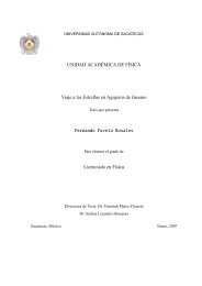
10 2 Differential geometry without a metricSince we are primarily concerned with specific applications, we shall emphasizethe rules of manipulation and calculation in differential geometry.We do not attempt to provide a substitute for standard texts on the subject,e.g. Eisenhart (1927), Schouten (1954), Flanders (1963), Sternberg(1964), Kobayashiand Nomizu (1969), Schutz (1980), Nakahara (1990)and Choquet-Bruhat et al. (1991) to which the reader is referred for fullerinformation and for the proofs of many of the theorems. Useful introductionscan also be found in many modern texts on relativity.For the benefit of those familiar with the traditional approach to tensorcalculus, certain formulae are displayed both in coordinatefree form andin the usual component formalism.2.2 Differentiable manifoldsDifferentiable manifolds are the most basic structures in differential geometry.Intuitively, an (n-dimensional) manifold is a space M such thatany point p ∈Mhas a neighbourhood U⊂Mwhich is homeomorphicto the interior of the (n-dimensional) unit ball. To give a mathematicallyprecise definition of a differentiable manifold we need to introduce someadditional terminology.A chart (U, Φ) in M consists of a subset U of M together with a one-toonemap Φ from U onto the n-dimensional Euclidean space E n or an opensubset of E n ; Φ assigns to every point p ∈U an n-tuple of real variables,the local coordinates (x 1 ,...,x n ). As an aid in later calculations, we shallsometimes use pairs of complex conjugate coordinates instead of pairsof real coordinates, but we shall not consider generalizations to complexmanifolds (for which see e.g. Flaherty (1980) and Penrose and Rindler(1984, 1986)).Two charts (U, Φ), (U ′ , Φ ′ ) are said to be compatible if the combinedmap Φ ′ ◦ Φ −1 on the image Φ(U ∪U ′ ) of the overlap of U and U ′ isa homeomorphism (i.e. continuous, one-to-one, and having a continuousinverse): see Fig. 2.1.An atlas on M is a collection of compatible charts (U α , Φ α ) such thatevery point of M lies in at least one chart neighbourhood U α . In mostcases, it is impossible to cover the manifold with a single chart (an examplewhich cannot be so covered is the n-dimensional sphere, n>0).An n-dimensional (topological) manifold consists of a space M togetherwith an atlas on M. Itisa(C k or analytic) differentiable manifold Mif the maps Φ ′◦ Φ −1 relating different charts are not just continuousbut differentiable (respectively, C k or analytic). Then the coordinates arerelated by n differentiable (C k , analytic) functions, with non-vanishing

2.2 Differentiable manifolds 11UUMΦΦoΦ −1{x }{xΦi i }Fig. 2.1. Two compatible charts of a differentiable manifoldJacobian at each point of the overlap:x i′ = x i′ (x j ), det(∂x i′ /∂x j ) ̸= 0. (2.1)Definitions of manifolds often include additional topological restrictions,such as paracompactness and Hausdorffness, and these are indeed essentialfor the rigorous proof of some of the results we state, as is the precisedegree of smoothness, i.e. the value of k. For brevity, we shall omit anyconsideration of these questions, which are of course fully discussed in theliterature cited earlier.A differentiable manifold M is called orientable if there exists an atlassuch that the Jacobian (2.1) is positive throughout the overlap of any pairof charts.If M and N are manifolds, of dimensions m and n, respectively, the(m + n)-dimensional product M×N can be defined in a natural way.A map Φ : M → N is said to be differentiable if the coordinates(y 1 ,...,y n ) on V ⊂ N are differentiable functions of the coordinates(x 1 ,...,x n ) of the corresponding points in U⊂Mwhere Φ maps (a partof) the neighbourhood U into the neighbourhood V. If Φ(M) ̸= N ,Φ(M) is called a submanifold of N : submanifolds P⊂Nof dimensionp

12 2 Differential geometry without a metricpoγ(t)ΦΦ( p )oΦ(γ(t))M (1x , . . . , x )N ( y , . . . , yn 1n)Fig. 2.2. The map of a smooth curve γ(t) toΦ(γ(t))2.3 Tangent vectorsIn general a vector cannot be considered as an arrow connecting twopoints of the manifold. To get a consistent generalization of the conceptof vectors in E n , one identifies vectors on M with tangent vectors. Atangent vector v at p isanoperator (linear functional) which assigns toeach differentiable function f on M a real number v(f). This operatorsatisfies the axioms(i) v(f + h) =v(f)+v(h),(ii) v(fh)=hv(f)+fv(h),(iii) v(cf) =cv(f), c = const.(2.2)It follows from these axioms that v(c) = 0 for any constant function c.The definition (2.2) is independent of the choice of coordinates. A tangentvector is just a directional derivative along a curve γ(t) through p: expandingany function f in a Taylor series at p, and using the axioms (2.2), onecan easily show that any tangent vector v at p can be written asv = v i ∂/∂x i . (2.3)The real coefficients v i are the components of v at p with respect to thelocal coordinate system (x 1 ,...,x n ) in a neighbourhood of p. Accordingto (2.3), the directional derivatives along the coordinate lines at p forma basis of an n-dimensional vector space the elements of which are thetangent vectors at p. This space is called the tangent space T p . The basis{∂/∂x i } is called a coordinate basis or holonomic frame.A general basis {e a } is formed by n linearly independent vectors e a ;any vector v ∈ T p is a linear combination of these basis vectors, i.e.v = v a e a . (2.4)The action of a basis vector e a on a function f is denoted by the symbolf |a ≡ e a (f). In a coordinate basis we use a comma in place of a solidus,f ,i ≡ ∂f/∂x i . A non-singular linear transformation of the basis {e a }

2.4 One-forms 13induces a change of the components v a of the vector v,e a ′ = L a ′ b e b , v a′ = L a′ bv b , L a′ bL a ′ c = δ c b. (2.5)A coordinate basis {∂/∂x i } represents a special choice of {e a }. In the olderliterature on general relativity the components with respect to coordinatebases were preferred for actual computations. However, for many purposesit is more convenient to use a general basis, often called a frame or n-bein(in four dimensions, a tetrad or vierbein), though when there is a metric,as in Chapter 3, these terms may be reserved for the cases with constantlengths. Well-known examples are the Petrov classification (Chapter 4)and the Newman–Penrose formalism (Chapter 7).The set of all tangent spaces at points p in M forms the tangent bundleT (M) ofM. To make this a differentiable manifold, the charts on T (M)can be defined by extending the charts (U, Φ) of M to charts (U ×R n , Φ×Id) where Id is the identity map on R n , i.e. we can use the components(2.3) to extend coordinates x i on M to coordinates (x i ,v j )onT (M). Thetangent bundle thus has dimension 2n. IfM isaC k manifold, T (M) isC k−1 .We can construct a vector field v(p) onM by assigning to each pointp ∈Ma tangent vector v ∈ T p so that the components v i are differentiablefunctions of the local coordinates. Thus a vector field can beregarded as a smooth map M→T (M) such that each point p → v(p),and is then referred to as a section of the tangent bundle.From the identification of vectors with directional derivatives one concludesthat in general the result of the successive application of two vectorsto a function depends on the order in which the operators are applied.The commutator [u, v] of two vector fields u and v is defined by[u, v](f) =u(v(f)) − v(u(f)). For a given basis {e a }, the commutators[e a , e b ]=D c abe c , D c ab = −D c ba, (2.6)define the commutator coefficients D c ab, which obviously vanish for a coordinatebasis: [∂/∂x i , ∂/∂x j ] = 0. Commutators satisfy the Jacobi identity[u, [v, w]]+[v, [w, u]]+[w, [u, v]] = 0 (2.7)for arbitrary u, v, w, from which one infers, for constant D c ab, the identityD f d[aD d bc] =0. (2.8)2.4 One-formsBy definition, a 1-form (Pfaffian form) σ maps a vector v into a realnumber, the contraction, denoted by the symbol 〈σ, v〉 or v σ, and this

14 2 Differential geometry without a metricmapping is linear:〈σ,au + bv〉 = a〈σ, u〉 + b〈σ, v〉 (2.9)for real a, b, and u, v ∈ T p . Linear combinations of 1-forms σ, τ aredefined by the rule〈aσ + bτ , v〉 = a〈σ, v〉 + b〈τ , v〉 (2.10)for real a, b. The n linearly independent 1-forms ω a which are uniquelydetermined by〈ω a , e b 〉 = δ a b (2.11)form a basis {ω a } of the dual space T ∗ p of the tangent space T p . This basis{ω a } is said to be dual to the basis {e b } of T p . Any 1-form σ ∈ T ∗ p isalinear combination of the basis 1-forms ω a ;σ = σ a ω a . (2.12)For any σ ∈ T ∗ p , v ∈ T p the contraction 〈σ, v〉 can be expressed in termsof the components σ a , v a of σ, v with respect to the bases {ω a }, {e a } by〈σ, v〉 = σ a v a . (2.13)The differential df of an arbitrary function f is a 1-form defined by theproperty〈df,v〉 = v(f) ≡ v a f |a . (2.14)Specializing this definition to the functions f = x 1 ,...,x n one obtainsthe relation〈dx i , ∂/∂x j 〉 = δ i j, (2.15)indicating that the basis {dx i } of Tp∗ is dual to the coordinate basis{∂/∂x i } of T p . Any 1-form σ ∈ Tp∗ can be written with respect to thebasis {dx i } asσ = σ i dx i . (2.16)In local coordinates, the differential df has the usual formdf = f |a ω a = f ,i dx i . (2.17)From 1-forms at points in M we can build the 1-form bundle T ∗ (M)of M, also called the cotangent bundle of M, and define fields of 1-formson M, analogously to the constructions for vectors, the components σ iof a 1-form field being differentiable functions of the local coordinates.In tensor calculus the components σ i are often called ‘components of acovariant vector’.

2.5 Tensors 152.5 TensorsA tensor T of type (r, s), and of order (r + s), at p is an element of theproduct spaceT p (r, s) =T p ⊗···⊗T p ⊗ Tp ∗ ⊗···⊗Tp∗ } {{ } } {{ }r factorss factorsand maps any ordered set of r 1-forms and s vectors,(σ 1 ,...,σ r ; v 1 ,...,v s ), (2.18)at p into a real number. In particular, the tensor u 1 ⊗···⊗u r ⊗ τ 1 ⊗··· ⊗ τ s maps the ordered set (2.18) into the product of contractions,〈σ 1 , u 1 〉···〈σ r , u r 〉〈τ 1 , v 1 〉···〈τ s , v s 〉. The map is multilinear, i.e. linearin each argument. In terms of the bases {e a }, {ω b } an arbitrary tensor Tof type (r, s) can be expressed as a sum of tensor productsT = T a 1···a r b1···b se a1 ⊗···⊗e ar ⊗ ω b1 ···⊗ω bs , (2.19)where all indices run from 1 to n. The coefficients T a 1···a r b1···b swith covariantindices b 1 ···b s and contravariant indices a 1 ···a r are the componentsof T with respect to the bases {e a }, {ω b }. For a general tensor, the factorsin the individual tensor product terms in (2.19) may not be interchanged.Non-singular linear transformations of the bases,e a ′ = L a ′ a e a , ω a′ = L a′ aω a , L a′ bL a ′ c = δ c b, (2.20)change the components of the tensor T according to the transformationlawT a′ 1···a′ r ′ b= L a′1···b′ 1 a1 ···L a′ r b1 bar Lsb ′1···L s b ′ sT a 1···a r b1···b s. (2.21)For transformations connecting two coordinate bases {∂/∂x a }, {∂/∂x a′ },the (n × n) matrices L a′ a, L a ′ a take the special forms L a′ a = ∂x a′ /∂x a ,L a ′ a = ∂x a /∂x a′ .The following algebraic operations are independent of the basis usedin (2.19): addition of tensors of the same type, multiplication by a realnumber, tensor product of two tensors, contraction on any pair of one contravariantand one covariant index, and formation of the (anti)symmetricpart of a tensor.Maps of tensors. The map Φ (Fig. 2.2) sending p ∈Mto Φ(p) ∈Ninduces in a natural way a map Φ ∗ of the real-valued functions f definedon N to functions on M,Φ ∗ f(p) =f(Φ(p)). (2.22)

16 2 Differential geometry without a metricMoreover, induced maps of vectors and 1-formsΦ ∗ : v ∈ T p → Φ ∗ v ∈ T Φ(p) ,Φ ∗ : σ ∈ T ∗ Φ(p) → Φ∗ σ ∈ T ∗ p ,(2.23)are defined by the postulates:(i) the image of a vector satisfiesΦ ∗ v(f)| Φ(p) = v(Φ ∗ f)| p ,(2.24a)Φ ∗ v being the tangent vector to the image curve Φ(γ(t)) at Φ(p), if v isthe tangent vector to γ(t) atp (see Fig. 2.2);(ii) the maps (2.23) preserve the contractions,〈Φ ∗ σ, v〉| p = 〈σ, Φ ∗ v〉| Φ(p) . (2.24b)It follows immediately from (2.24a) that, for any u and v,[Φ ∗ u, Φ ∗ v]=Φ ∗ [u, v]. (2.25)Let us denote local coordinates in corresponding neighbourhoods ofp and Φ(p) by(x 1 ,...,x m ) and (y 1 ,...,y n ) respectively. The map of a1-form σ is given simply by coordinate substitution,(Φ ∗ : σ = σ i (y)dy i → Φ ∗ σ = σ i (y(x)) ∂y i /∂x k) dx k = ˜σ k (x)dx k ,(2.26)i =1,...,n, k =1,...,m.These maps can immediately be extended to tensors of arbitrary type(r, s) provided that the inverse Φ −1 exists, i.e. that Φ is a one-to-onemap. In this case, (2.24b) can be rewritten in the form〈Φ ∗ σ, Φ −1∗ v〉| p = 〈σ, v〉| Φ(p) . (2.27)Note that Φ ∗ maps tensors on N to tensors on M, starting from a mapΦofM to N . Although (2.26) looks like a coordinate transformation, itdefines new tensors, Φ ∗ σ etc. In contrast, under the transformation (2.20)of the basis of a given manifold M any tensor remains the same object;only its components are changed. Tensors are invariantly defined.Up to now we have considered tensors at a given point p. The generalizationto tensor bundles and tensor fields is straightforward. As specialcases we have defined fields of 1-forms and vector fields on M at theends of §§2.3 and 2.4. In the next few sections we shall introduce variousderivatives of tensor fields. For brevity, we shall call tensor fields simplytensors.

2.6 Exterior products and p-forms 172.6 Exterior products and p-formsLet α 1 ,...,α p denote p 1-forms. We define an algebraic operation ∧, theexterior product or wedge product (up to a factor) by the axioms: theexterior product α 1 ∧ α 2 ∧···∧α p(i) is linear in each variable, and(ii) vanishes if any two factors coincide.From these axioms it follows that the exterior product changes sign if anytwo factors are interchanged, i.e. it is completely antisymmetric. From thebasis 1-forms ω 1 ,...,ω n we obtain ( np) independent p-formsω a 1∧···∧ω ap , 1 ≤ a 1

18 2 Differential geometry without a metricso that the p-forms are precisely the antisymmetric tensors of type (0,p)(antisymmetric covariant tensors). The factor of proportionality is fixedby the rule that if α and β have the components α a1···a pand β b1···b q,(p)(q)respectively, then their exterior product has the components( )α ∧ β a 1···a pb 1···b q= α [a1···a pβ b1···b q], (2.34)(p) (q)which leads, for example, to ω 1 ∧ ω 2 =(ω 1 ⊗ ω 2 − ω 2 ⊗ ω 1 )/2. Thecomponent form of (2.33) is thenA p-form α(p)(v α ) a2···a p= v b α ba2···a p. (2.35)(p)is said to be simple if it admits a representation as anexterior product of p linearly independent 1-forms,α = α 1 ∧ α 2 ∧···∧α p . (2.36)(p)2.7 The exterior derivativeIn §2.4 we defined the differential df of a function f by the equation(2.14). The operator d generates a 1-form df from a 0-form f byd:f → df = f ,i dx i . (2.37)We generalize this differentiation to apply to any p-form. The exteriorderivative d maps a p-form into a (p + 1)-form and is completely determinedby the axioms:(i) d(α + β) =dα +dβ, (2.38a)( )(ii) d α ∧ β =dα ∧ β +(−1) p α ∧ d β , (2.38b)(p) (q) (p) (q)(p) (q)(iii) df = f ,i dx i , (2.38c)(iv) d(df) =0. (2.38d)Because of axiom (2.38a) it is sufficient to verify the existence and uniquenessof the exterior derivative for the p-form fdx i 1∧···∧dx ip . One canprove (see e.g. Flanders (1963)) thatd(fdx i 1∧···∧dx ip )=df ∧ dx i 1∧···∧dx ip . (2.39)and that all the axioms (2.38) are then satisfied.

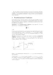
2.7 The exterior derivative 19From a general p-form (2.30) we obtain the (p + 1)-formd α = α i1···i p,jdx j ∧ dx i 1∧···∧dx ip (2.40)(p)by exterior differentiation. The (completely antisymmetric) componentsof d α involve only partial derivatives of the components α i1···i p.Weremarkthat axiom (2.38d) is just the equality of the mixed second partial(p)derivatives of f,From (2.40) we see thatd(df) =d(f ,i dx i )=f ,i,j dx j ∧ dx i =0. (2.41)d(dα) = 0 (2.42)for any p-form α.The following theorems, for proofs of which we refer the reader to theliterature (e.g. for Theorem 2.2 see Flanders (1963)), hold locally, i.e. ina neighbourhood of a point p.Theorem 2.1 (Poincaré’s theorem). If α is a p-form (p ≥ 1) anddα =0, then there is a (p − 1)-form β such that α =dβ. In components,α [i1···i p,j] =0 ⇔ α i1···i p= β [i1···i p−1 ,i p]. (2.43)Theorem 2.2 (Frobenius’s theorem). Let σ 1 ,...,σ r be r 1-forms linearlyindependent at a point p ∈ M. Suppose there are 1-forms τ A B(A, B =1,...,r) satisfying dσ A = τ A B ∧ σ B . Then in a neighbourhoodof p there are functions f A B, h A such that σ A = f A Bdh B .Other formulations of Frobenius’s theorem. Introducing the r-form Σ ≡σ 1 ∧···∧σ r , we can replace the condition dσ A = τ A B ∧ σ B by either ofthe two equivalent conditions:(i) dσ A ∧ Σ =0,(ii) there exists a 1-form λ such that dΣ = λ ∧ Σ.In the case of a single 1-form σ we have the resultor in components,σ ∧ dσ =0⇔ σ = fdh, (2.44)σ [a,b σ c] =0⇔ σ a = fh ,a . (2.45)The surfaces h = constant are called the integral surfaces of the equationσ =0,f −1 being the integrating factor.

20 2 Differential geometry without a metricFrobenius’s theorem is important in the construction of exact solutionsbecause it allows us to introduce local coordinates f, h adapted to givennormal 1-forms (see e.g. §27.1.1).The rank q of a 2-form α is defined byα ∧···∧α} {{ }q factors̸= 0, α} ∧···∧α {{ } =0, 2q ≤ n. (2.46)(q+1) factorsUsing this definition we can generalize the statement (2.44) toTheorem 2.3 (Darboux’s theorem). Let σ be a 1-form and let the 2-formdσ have rank q. Then we can find local coordinates x 1 ,...,x q , ξ 1 ,...,ξ n−qsuch that{ =0:σ = x 1 dξ 1 + ···+ x q dξ q ,if σ ∧ dσ } ∧···∧dσ {{ } ̸= 0:σ = x 1 dξ 1 + ···+ x q dξ q +dξ q+1 (2.47).q factors(For a proof, see Sternberg (1964).)This theorem gives the possible normal forms of a 1-form σ. SpecializingDarboux’s theorem to a four-dimensional manifold one obtains thefollowing classification of a 1-form σ in terms of its components:q =0:σ [a,b] =0: σ a = ξ ,aq =1:σ [a,b] ̸= 0, σ [a,b σ c,d] =0,σ [a,b σ c] =0:σ a = xξ ,aσ [a,b] ̸= 0, σ [a,b σ c,d] =0,σ [a,b σ c] ̸= 0:σ a = xξ ,a + η ,a(2.48)q =2:σ [a,b σ c,d] ̸= 0 σ a = xξ ,a + yη ,a .The real functions denoted by x, y, ξ, η are independent. The secondsubcase is just Frobenius’s theorem applied to a single 1-form σ.Now we give a theorem concerning 2-forms.Theorem 2.4 For any 2-form α of rank q there exists a basis {ω a } suchthatα =(ω 1 ∧ ω 2 )+(ω 3 ∧ ω 4 )+···+(ω 2q−1 ∧ ω 2q ). (2.49)If dα =0, then we can introduce local coordinates x 1 ,...,x q , ξ 1 ,...,ξ n−qsuch thatα =dx 1 ∧ dξ 1 + ···+dx q ∧ dξ q . (2.50)(For a proof, see Sternberg (1964).)To conclude this series of theorems, we consider a map Φ : M→Nbetween two manifolds, as in (2.23), and show by induction

2.8 The Lie derivative 21Theorem 2.5 For the exterior derivative dα of a p-form α we haved(Φ ∗ α)=Φ ∗ (dα). (2.51)Proof: Let us denote local coordinates in corresponding neighbourhoodsof p ∈Mand Φ(p) ∈N by (x 1 ,...,x m ) and (y 1 ,...,y n ) respectively.Obviously, (2.51) is true for a 0-form f:d(Φ ∗ f)= ∂(Φ∗ f)∂x kdx k = ∂f(y(x))∂y i∂y i∂x k dxk =Φ ∗ (df). (2.52)Suppose the relation is valid for the (p − 1)-form β and let α = fdβ.(This is sufficiently general.) Then,d(Φ ∗ α) = d[(Φ ∗ f)d(Φ ∗ β)] = d(Φ ∗ f) ∧ d(Φ ∗ β)=Φ ∗ (dα). (2.53)We do not consider integration on manifolds, except to note that theoperator d of exterior derivation has been defined so that Stokes’s theoremcan be written in the simple form∫ ∫α = dα, (2.54)∂Vwhere α isany(k −1)-form and ∂V denotes the oriented boundary of a k-dimensional manifold with boundary V. (An n-dimensional manifold withboundary is defined by charts which map their neighbourhoods U into thehalf space H n defined by x n ≥ 0 rather than into E n , the boundary thenbeing the set of points mapped to x n = 0.)V2.8 The Lie derivativeFor each point p ∈M, a vector field v on M determines a unique curveγ p (t) such that γ p (0) = p and v is the tangent vector to the curve. Thefamily of these curves is called the congruence associated with the vectorfield. Along a curve γ p (t) the local coordinates (y 1 ,...,y n ) are thesolutions of the system of ordinary differential equationsdy idt = vi (y 1 (t),...,y n (t)) (2.55)with the initial values y i (0) = x i (p).To introduce a new type of differentiation we consider the map Φ t draggingeach point p, with coordinates x i , along the curve γ p (t) through p intothe image point q =Φ t (p) with coordinates y i (t). For sufficiently smallvalues of the parameter t the map Φ t is a one-to-one map which induces

22 2 Differential geometry without a metrica map Φ ∗ t T of any tensor T , called Lie transport. The Lie derivative ofT with respect to v is defined by1LvT ≡ limt→0 t (Φ∗ t T − T ). (2.56)The tensors T and Φ ∗ t T are of the same type (r, s) and are both evaluatedat the same point p. Therefore, the Lie derivative (2.56) is also a tensorof type (r, s) atp. The Lie derivative vanishes if the tensors T and Φ ∗ t Tcoincide. In this case the tensor field T remains in a sense the ‘same’ underLie transport along the integral curves of the vector field v. However,the components of T with respect to the coordinate basis {∂/∂x i } mayvary along the curves. Using coordinate bases {∂/∂x i } and {∂/∂y i },wecompute the components of the Lie derivative. The relations∂y i∂x k ∣ ∣∣∣∣t=0= δ i k,dy idt= v i ,∣ t=0dx idt= −v i (2.57)∣ t=0will be used. We start with the Lie derivatives of functions, 1-forms, andvectors:function f: Lvf = v i f, i (= v(f)). (2.58)Proof:Φ ∗ t f| p = f(y(x, t)),Lvf| p = ∂fdy i∂y i .dt ∣ p1-form σ: Lvσ =(v m σ i,m + σ m v m ,i)dx i . (2.59)Proof:vector u:Proof:Φ ∗ t σ| p = σ j (y(x, t)) ∂yj∂x i dxi ,[∂σj dy m ∂y j ( )]Lvσ| p =∂y m dt ∂x i + σ ∂ dyjj∂x i dtt=0dx i .Lvu =(v m u i ,m − u m v i ,m) ∂∂x i . (2.60)Φ ∗ t u| p = u j (y(x, t)) ∂xi ∂∂y j ∂x i ,[∂ujdy m ∂x i ( )]Lvu| p =∂y m dt ∂y j + ∂ dxiuj∂y j dtt=0∂∂x i .

2.9 The covariant derivative 23The Lie derivative of u with respect to v is equal to the commutator[v, u],Lvu =[v, u] =v m ∂ ( )∂x m u i ∂∂x i − u m ∂ ( )∂x m v i ∂∂x i . (2.61)Two commuting vector fields generate a family of two-dimensional submanifoldsof M on which the parameters of the integral curves of bothvector fields can be taken as coordinates.From the Leibniz product rule and (2.59), (2.60) one obtains the componentsof the Lie derivative of an arbitrary tensor,(LvT ) ij···kl··· = v m T ij···kl···,m − T mj···kl···v i ,m − T im···kl···v j ,m −···+ T ij···ml···v m ,k + T ij···km···v m ,l + ··· . (2.62)Equation (2.61) and the Jacobi identity (2.7) imply that when applied tovectorsL u L v −L v L u = L [u, v] , (2.63)and (2.58) and the Leibniz rule then imply that this is true for any tensor.From (2.51), (2.56), it follows that the Lie derivative applied to formscommutes with the exterior derivative:d(Lvα) =Lv(dα) (2.64)for any p-form α. Of course, this rule can also be verified by using (2.40),(2.62) in terms of components.As will be seen later, the Lie derivative plays an important role indescribing symmetries of gravitational fields and other physical fields.The exterior derivative and the Lie derivative are operations defined ona differentiable manifold without imposing additional structures. Both operationsare generalizations of the partial derivative. The exterior derivativeis a limited generalization acting only on forms. The Lie derivativedepends on the vector v not only at p, but also at neighbouring points.To introduce invariantly defined derivatives which have neither of thesedefects we have to impose a new structure on M, and we proceed to doso in the following section.2.9The covariant derivativeThe covariant derivative ∇v in the direction of the vector v at p mapsan arbitrary tensor into a tensor of the same type. If v is unspecified, thecovariant derivative ∇ generates a tensor of type (r, s + 1) from a tensorof type (r, s). In particular, for a vector u we have the expansion∇u = u a ;be a ⊗ ω b (2.65)

24 2 Differential geometry without a metricwith components u a ;b as yet unspecified. The directional covariant derivativeis given by the vector∇vu =(u a ;bv b )e a . (2.66)The covariant derivative of the basis vector e a in the direction of the basisvector e b can be expanded in terms of basis vectors:∇ b e a =Γ c abe c , Γ c ab = 〈ω c , ∇ b e a 〉. (2.67)For consistency of (2.67) with the Leibniz rule applied to (2.11), the covariantderivative of a dual basis {ω a } is given by∇ b ω a = −Γ a cbω c . (2.68)The coefficients Γ c ab, called the connection coefficients, relate the bases atdifferent points of M, and they have to be imposed as an extra structureon M. We restrict ourselves to covariant derivatives satisfying∇uv −∇vu =[u, v] (2.69)for two arbitrary vectors u and v. This relation is equivalent to the equation2Γ c [ab] = −D c ab, (2.70)where the commutation coefficients are defined by (2.6). In a coordinatebasis, the connection coefficients Γ c ab have a symmetric index pair (ab).Therefore a covariant derivative satisfying (2.69) is called symmetric (ortorsionfree).Using the symmetry axiom (2.70), we may replace the partial derivativesin (2.40) and (2.62) for the components of, respectively, the exteriorderivative and the Lie derivative by covariant derivatives, so that thecommas can be replaced by semicolons.Once the connection coefficients are prescribed, the components u a ;c ofthe covariant derivative of u in the direction of the basis vector e c arecompletely determined,∇ c u = ∇ c (u a e a )=(u a |c +Γ a dcu d )e a = u a ;ce a ,(2.71a)and the components of the covariant derivative ∇T of a tensor (2.19) areT a 1···a r b1···b s;c =(T a 1···a r b1···b s) |c +Γ a 1 dc T d···ar b 1···b s+ ···+Γ ar dcT a 1···d b1···b s−Γ d b 1 cT a 1···a r d···bs −···−Γ d b scT a 1···a r b1···d,(2.71b)where the symbol f |a ≡ e a (f) =f ,i e a i has been used. Note that (2.71b)is valid for a general basis {e a }.

2.10 The curvature tensor 25Since the bases {e a }, {ω a } are linear combinations of coordinate bases,e a = e a i ∂/∂x i , ω a = ω a idx i , (2.72)the connection coefficients (2.67) can be written with respect to thesebases asΓ c ab = ω c kke a ;i e i b = −e k a ω c k;ie i b . (2.73)These are also referred to as the Ricci rotation coefficients. For the exteriorderivative of the basis 1-forms we getdω a = ω a i,jdx j ∧ dx i = ω a i;jdx j ∧ dx i =Γ a bcω b ∧ ω c . (2.74)Introducing the connection 1-formswe can write (2.74) in the formΓ a b ≡ Γ a bcω c , (2.75)dω a = −Γ a b ∧ ω b (2.76)due to Cartan (the first Cartan equation). For a given basis, the antisymmetricpart Γ a [bc] of the connection coefficients can be computed fromthis.The definition of the covariant derivative is equivalent to a definitionof parallellism; the relation is that if w(q) is the vector at q parallel tou(p) atp, and v(p) is the tangent vector at p to a curve γ from p = γ(0)to q = γ(ɛ), the covariant derivative ∇vu is the limit of [w(q) − u(q)]/ɛas ɛ → 0. Thus, a tensor T is said to be parallelly-transported along thecurve with tangent vector v if ∇vT =0.Anautoparallel curve is onewhose tangent vector is parallel to itself along the curve.2.10 The curvature tensorThe curvature tensor (Riemann tensor), R = R a bcde a ⊗ ω b ⊗ ω c ⊗ ω d isa tensor of type (1, 3) mapping the ordered set (σ; w,u,v) of a 1-form σand three vectors w,u,v into the real numberσ a w b u c v d R a bcd = 〈σ, (∇u∇v −∇v∇u −∇ [u,v])w〉= σ a [(w a ;cv c ) ;d u d − (w a ;cu c ) ;d v d − w a ;c(u d v c ;d − v d u c ;d)]= σ a (w a ;cd − w a ;dc)v c u d . (2.77)As the components σ a , v c , u d can be chosen arbitrarily we arrive at theRicci identityw a ;cd − w a ;dc = w b R a bdc. (2.78)

26 2 Differential geometry without a metricThe general rules (2.71) for the components of the covariant derivative ofa tensor imply the formulaR a bcd =Γ a bd|c − Γ a bc|d +Γ e bdΓ a ec − Γ e bcΓ a ed − D e cdΓ a be. (2.79)In a coordinate basis, the last term vanishes. The components (2.79) ofthe curvature tensor satisfy the symmetry relationsR a bcd = −R a bdc, R a [bcd] =0. (2.80)The covariant derivatives of the curvature tensor obey the BianchiidentitiesR a b[cd;e] =0. (2.81)By contraction we obtain the identitiesR a bcd;a +2R b[c;d] =0, (2.82)where the components R bd of the Ricci tensor are defined byR bd ≡ R a bad. (2.83)If a vector is parallelly transported round a closed curve, the initialand final vectors will in general not be equal: this phenomenon is calledholonomy. For infinitesimally small curves the holonomy is given by anintegral of the curvature tensor over an area enclosed by the curve, andconversely this gives an alternative way to define curvature.A compact and efficient method for calculating the components (2.79)with respect to a general basis is provided by Cartan’s procedure. Definingthe curvature 2-forms Θ a b byΘ a b ≡ 1 2 Ra bcdω c ∧ ω d , (2.84)equation (2.79) is completely equivalent to the second Cartan equationdΓ a b + Γ a c ∧ Γ c b = Θ a b, (2.85)which gives an algorithm for the calculation of the curvature from the connection.We collect the relations between the various quantities in Fig. 2.3.In this notation the Bianchi identities (2.81) are the components ofd 2 Γ a b =dΘ a b − Θ a c ∧ Γ c b + Γ a c ∧ Θ c b =0. (2.86)

2.11 Fibre bundles 27Γ a bc (2.79) ✲ R a bcd✻✻(2.75)(2.84)❄❄Γ a b (2.85) ✲ Θ a bFig. 2.3. How to get the curvature from the connection2.11 Fibre bundlesThe tensor bundles introduced in §2.4 are examples of fibre bundles. Asimple picture of a fibre bundle E over a manifold M can be obtainedby imagining a copy of another manifold F, the fibre, to be attached toeach point of M in such a way that for suitable regions where coordinatesx j are given on M and ξ a on the fibre, the fibre bundle has coordinates(x j ,ξ a ), i.e. E is locally M×F; M is called the base manifold. On regionswhere two coordinate systems in M apply, the corresponding coordinatetransformations of E are given by the usual coordinate transformations inM together with fibre transformations ξ b′ = ξ b′ (ξ a ) for each p ∈M; thesefibre transformations belong to a group of transformations of F calledthe structure group of the bundle. (For the tangent bundle the structuregroup just consists of linear transformations of R m .) The structure groupis often a Lie group G, as defined in Chapter 8. (For fuller details, see e.g.Steenrod (1951), Crampin and Pirani (1986).)The map π : E→M;(p, f) ↦→ p is called the projection onto the basemanifold M. Amapσ : M→Ewhich for each point p in M gives aunique point σ(p) ∈ π −1 (p) is called a section, consistently with the useof this term above. All the maps involved in the definition must of coursebe suitably smooth. If F is a vector space, the bundle is called a vectorbundle.The frame bundle F (M) for a manifold M has as the fibre F at p the setof all possible bases of T p (M), so the structure group is the group of nonsingularlinear transformations GL(n, R). Similarly T ∗ p (M) defines thecoframe bundle. Various restricted (co)frame bundles can be obtained byrestricting the set of allowed (co)frames, the most common case, in spacetimes,being restriction to one of the special classes of tetrads, orthonormalor null (see Chapter 3). In frame bundles the structure group and the fibrecan be identified, F ∼ = G, i.e. each choice of frame can be obtained byapplying a unique element of the structure group to a basic choice of

28 2 Differential geometry without a metricframe: a bundle with this property is called a principal bundle. Framebundles play an essential role in the theory underlying Cartan’s methodfor testing equivalence of metrics (see Chapter 9).Given a point in p ∈ F (M) and any tangent vector v at π(p) ∈M,tangent to a curve γ(t) say, we can use the connection to define theparallelly-transported frame at neighbouring points of γ(t), i.e. to definea corresponding lifted curve in F (M). The set of all such lifted curvesdefines an n-dimensional plane at p, called horizontal, and the tangentto the lifted curve at p defines a vector in T (F M)), the horizontal lift ofv. The distribution of horizontal subspaces in fact completely defines theconnection. The basis corresponding to p can be lifted to give a uniquelydefined basis of horizontal vectors at p. One-forms on M can be lifted tothe horizontals in F (M) byπ ∗ ;atapointp, they have a uniquely-definedbasis given by lifting the basis of 1-forms dual to the basis defined by p.Now consider a general curve through p ∈ F (M) with tangent vectorV , and a frame {e a }. The change of frame along the horizontal part ofV , defined by π ∗ (V ), is given by the usual connection, while the changedue to the vertical part of V , i.e. the part tangent to the fibre, is given by(2.5) with L a b = ̂Γ b acV c , where ̂Γ b ac depends on the parametrization ofGL(n, R). The quantities ̂Γ b ac can be added to Γ b ac to define a connectionΓ a b on the bundle; the formulae for covariant derivatives given in §2.9, inparticular (2.76), can then all be extended to F (M). Moreover, given theconnection (and the structure group) the 1-form fields ω a and Γ a b area uniquely defined basis on F (M). Similar remarks apply to the variousrestricted (co)frame bundles.From this connection, one can define a curvature in F (M). Direct calculationshows (see e.g. Araujo et al. (1992)) that the non-zero componentsof the curvature of F (M) atp are just given by those of the usualcurvature at π(p) in the frame {e a } which p represents, and (2.85) stillapplies although Γ a b and Θ a b now refer to the connection and curvatureon F (M). Part of the reason is that since the action of the structuregroup on a fibre maps the horizontal subspaces to one another in a uniqueway, transport in the vertical direction has no holonomy and correspondinglycomponents of the curvature in the vertical direction are zero. Oneshould note that the curvature components are invariantly-defined scalarson F (M) since they are known for a given point in M and frame.The exterior derivative of the components of curvature on F (M) obeysdR abcd = R abcd;e ω e +R ebcd Γ e a+R aecd Γ e b+R abed Γ e c+R abce Γ e d , (2.87)where R abcd;e is evaluated, in the tetrad given by p, atπ(p) ∈M, andsimilar equations hold for higher derivatives.

2.11 Fibre bundles 29Jet bundles J (n) (X, U) are another type of fibre bundle of interest inexact solutions (see Chapter 10). They are used in describing systemsof differential equations. Here the base manifold X is the space of independentvariables and the fibre is the set U of values of the dependentvariables and their first n partial derivatives with respect to the X. A(partial) differential equation, or a system of such equations, specifies asubmanifold in a jet bundle.

3Some topics in Riemannian geometry3.1 IntroductionIn Chapter 2 we treated differential geometry without a metric. In orderto define covariant derivatives we imposed an extra structure on thedifferential manifold M, the connection. Adding a further structure, themetric g ab , and postulating g ab;c = 0, we arrive at Riemannian geometry.General relativity is based on the concept of space-time, which is a fourdimensionaldifferentiable (C ∞ , Hausdorff) manifold M endowed with aLorentzian metric g ab which can be transformed tog ab = η ab ≡ diag(1, 1, 1, −1) (3.1)at any point of M, i.e. space-time is a normal-hyperbolic Riemannianspace V 4 . In what follows, a knowledge of fundamental facts about Riemanniangeometry as given in most textbooks on general relativity is presumed;we give here only some notation and results used in the remainderof this book. For further details the reader is referred to standard textson Riemannian geometry, e.g. Eisenhart (1949) and Schouten (1954).3.2 The metric tensor and tetradsWe introduce as a new structure a symmetric tensor of type (0,2), calledthe metric tensor g, which endows each vector space T p with a scalarproduct (inner product)e a · e b = g ab . (3.2)The tensor g, sometimes called the line element ds 2 , is writteng =ds 2 = g ab ω a ω b . (3.3)30

3.2 The metric tensor and tetrads 31The scalar product of two vectors v, w is given byv · w = g ab v a w b . (3.4)Two vectors v, w are orthogonal if their scalar product vanishes. A nonzerovector v is said to be spacelike, timelike or null, respectively, whenthe product v · v = g ab v a v b is positive, negative or zero. In a coordinatebasis, we write the line element ds 2 asds 2 = g ij dx i dx j . (3.5)The contravariant components, g ab , form the matrix inverse to g ab . Raisingand lowering the indices of the tensor components has to be performed inthe usual manner:v a = g ab v b , v a = g ab v b . (3.6)In this sense, the vector v a e a and the 1-form v a ω a represent the samegeometric object.In space-time, an orthonormal basis or orthonormal tetrad or Lorentzframe {E a } consists of three spacelike vectors E α and one timelike vectorE 4 ≡ t, such that{E a } = {E α , t} = {x, y, z, t}, g ab = x a x b + y a y b + z a z b − t a t b(3.7)⇔ E α · E β = δ αβ , t · t = −1, E α · t =0.If one has a fluid with four-velocity parallel to t, the symbol t is oftenreplaced by u.Complex null tetrads play an important role. A complex null tetradconsists of two real null vectors k, l and two complex conjugate nullvectors m, m:{e a } =(m, m, l, k),⎛⎞01 0 0g ab =2m (a m b) − 2k (a l b) = ⎜ 1 0 0 0⎟⎝ 00 0−1 ⎠00−1 0(3.8)(g ab are the components of g with respect to the complex null tetrad), i.e.the scalar products of the tetrad vectors vanish apart fromk a l a = −1, m a m a =1. (3.9)

32 3 Some topics in Riemannian geometryIn terms of a coordinate basis, a complex null tetrad {e a } and its dual{ω a } will take the forme 1 = m i ∂∂x i , e 2 = m i ∂∂x i , e 3 = l i ∂∂x i , e 4 = k i ∂∂x i ;ω 1 = m i dx i , ω 2 = m i dx i , ω 3 = −k i dx i , ω 4 = −l i dx i .(3.10)The explicit expressions for the directional derivatives f |a of a function fwith respect to the complex null tetrad (3.8) aref |1 = f ,i m i , f |2 = f ,i m i , f |3 = f ,i l i , f |4 = f ,i k i . (3.11)An orthonormal tetrad (3.7) and a complex null tetrad (3.8) may berelated by√ √2 m = E1 − iE 2 , 2 m = E1 +iE 2 ,√ √ (3.12)2 l = E4 − E 3 , 2 k = E4 + E 3 .In flat space-time, (3.12) implies the relationsζ = 1 √2(x +iy), ¯ζ =1 √2 (x − iy), u = 1 √2(t − z), v = 1 √2(t + z), (3.13)between the null coordinates ζ, ¯ζ, u, v (adapted to the basis vectorsm = ∂ ζ , m = ∂¯ζ, l = ∂ u , k = ∂ v ) and the Minkowski coordinates x, y,z, t (adapted to the basis vectors E 1 = ∂ x , E 2 = ∂ y , E 1 = ∂ z , E 4 = ∂ t ).Here we have adopted the convention ∂ ζ = ∂/∂ζ etc. In some approachesthe coordinates ζ, ζ, u and v are considered as four independent complexvariables, thus leading to a complexification of Einstein’s field equationsand the task of regaining real cuts from its complex solutions. Sometimesalso the mixed form of a real null tetrad or half null tetrad (x, y, l, k) isused.Lorentz transformations give rise to the following changes of the basis(3.8):null rotations (l fixed),l ′ = l, m ′ = m + El, k ′ = k + Em + Em + EEl, E complex; (3.14)null rotations (k fixed),k ′ = k, m ′ = m + Bk, l ′ = l + Bm + Bm + BBl, B complex; (3.15)spatial rotations in the m–m-plane,m ′ =e iΘ m, Θ real; (3.16)

3.2 The metric tensor and tetrads 33special Lorentz transformations (boosts) in the k–l-plane,k ′ = Ak, l ′ = A −1 l, A > 0. (3.17)The transformations (3.14)–(3.17) contain six real parameters. The transformationspreserving the k-direction arek ′ = Ak, m ′ =e iΘ (m+Bk), l ′ = A −1 (l+Bm+Bm+BBk). (3.18)Symmetric connection coefficients (2.67) are uniquely determined byadding the metric condition∇g =0 ⇔ g ab;c =0=g ab|c − 2Γ (ab)c , Γ abc ≡ g ad Γ d bc. (3.19)Combining the metric condition (3.19) and the symmetry condition (2.70)one obtains the general formulaΓ abc = 1 2 (g ab|c+g ac|b −g bc|a +D cab +D bac −D abc ), D abc ≡ g ad D d bc, (3.20)expressing the connection coefficients in terms of the metric tensor andthe commutation coefficients. We mention two cases of special interest:coordinate basis (holonomic frame): D ijk =0: Γ i[jk] =0,Γ i jk ≡{ ijk} (= Christoffel symbols);constant metric (rigid frame): g ab|c =0: Γ (ab)c =0.In a holonomic frame, the connection coefficients Γ abc are symmetric inthe index pair (bc), while in a rigid frame they are antisymmetric in theindex pair (ab).When using tetrad methods for a rigid frame, it is common to calculatesimultaneously the components of the basis vectors for the essentialcoordinates of the metric under study and the connection (and hencecommutation) coefficients, which involve only those coordinates. In orderto obtain a coordinate form for the metric, one then has to integrate(2.6) successively for the remaining unknown coordinate components ofthe tetrad basis. The coordinates {y α } not appearing in the commutationcoefficients can be chosen so that the operators ∂ y α are the ‘constants ofintegration’ arising in this process. The relevant integrability conditionsare the Jacobi identities: for further discussion, in the null tetrad context,see §7.3.In §2.9 autoparallels were introduced. One can also consider geodesiccurves, those for which the total length, measured using the metric, isextremal. The tangent vector v of a geodesic satisfies∇ v v = fv; in components: v b v a ;b = fv a . (3.21)

The Outbreak of the Napoleonic Wars 15proposed its neutrality under the guarantee of a thirdparty, Naples. Britain considered the establishment of aNeapolitan garrison, to deter future French designs onMalta, a ridiculous proposition; pending the accession ofthe other Great Powers to an article guaranteeing the island’sindependence, later known as Article X, it ultimatelyacquiesced to the condition.Nevertheless, Britain was remiss in failing to evacuatethe island and admit the 2,000 men of the Neapolitan garrisonwithin the three-month period allowed after the signatureof the treaty. Britain promised France it wouldwithdraw. Britain had, moreover, failed to evacuate entirelyits garrison from Egypt; a portion of its troops had remainedin Alexandria since Egypt’s restoration to Turkey.It was not until the First Consul issued a demand for itscomplete withdrawal that Britain satisfied the conditionsof the treaty on this point.By the new year, a crisis in Anglo-French relations wasgrowing. Austria had already acceded to the article guaranteeingthe sovereignty and independence of Malta, andRussia, despite the conditional nature of its acceptance,was thought amenable to accession. In London, however,the prime minister contemplated retaining the island.Addington’s continued delay in removing British troopssoon amounted to an overt violation of the treaty; Francewas not prepared to let this pass unnoticed, and on 27 FebruaryTalleyrand reminded Lord Whitworth of Britain’ssolemn obligations. Only the accession of Russia to ArticleX and the election of a new Grand Master of the Order ofMalta were wanting, the foreign minister stated. Thus, thetime for delay afforded by a pretext for continued occupationwould soon come to an end.Although Britain had originally agreed to Malta’sevacuation in good faith, in the light of French depredationson the Continent since the signature of Amiens,Addington balked at relinquishing the island to an uncertainfate under a Neapolitan garrison, notwithstandingpledges from Russia, Prussia, Austria, and other powers toguarantee the island’s independence. Moreover, various reportsfrom British envoys, including Sir John Warren at St.Petersburg and the Earl of Elgin, former ambassador toTurkey, aroused suspicions at Downing Street that Francewas contemplating a renewal of its previous designs onTurkey. If these reports alone did not convince the cabinetto retain the garrison indefinitely, a report published in theMoniteur in January 1803 reconfirmed Addington’s convictionthat Malta’s evacuation would be catastrophic toBritish interests in the Mediterranean in general, to Egyptspecifically, and by extension, to India. Similarly, it reinforcedprevailing views within British political and publiccircles that Bonaparte’s ambitions were boundless.The report was the product of the mission of ColonelHorace Sébastiani, a French infantry (later cavalry) officer,who was temporarily charged as an envoy to Turkey. Sébastianiwas ordered to make extensive travels in Egypt, theLevant, and the Balkans on a mission in order, ostensibly, toacquire commercial information on these regions. Irrespectiveof its true purpose, the mission yielded valuable intelligenceon the state of defense of various Ottoman provincesfor purposes of future French conquest. The publication ofSébastiani’s report, in which, among other conclusions, heobserved that 6,000 troops could easily subdue Egypt, excitedindignation in Britain and resolved Addington to refusethe evacuation of Malta as agreed to at Amiens.Lord Whitworth was instructed in early February to informthe French government that Malta would be retainedin compensation for the extensive territorial gains acquiredby France since the signature of Amiens. These gains hadcompletely overturned the balance and stability that bothpowers had pledged to uphold. As the state of possessionhad been so radically altered, Britain reserved the right, thegovernment argued, to seek compensation on the basis ofdiplomatic precedence in international law and the assumedsanction of this principle by France. In view of French gainsin Holland, Switzerland, and Italy, Whitworth was instructedin early February that his country believed it consistentwith the terms of Amiens to claim for itself compensationin order to balance the threat to its security that thesecontinental acquisitions represented; in short, Britain demandeda counterweight to French gains. The Sébastiani report,moreover, suggested continued French designs onEgypt—a wholly unacceptable prospect in British eyes.Whitworth recapitulated these arguments to the foreignminister in mid-February. Talleyrand assured him thatFrance entertained no designs on Egypt or India and referredto Sébastiani’s mission as a strictly commercial venture.The First Consul, he continued, had no desire to disturbthe peace reached at Amiens, and he claimed thatFrench finances would not, in any event, enable him to wagewar. Finally, he expressed surprise that the British governmentshould hold any suspicion of French intentions.Within days, Napoleon had summoned Whitworth tothe Tuileries to explain his position in person. The FirstConsul enumerated the various provocations for which heheld Britain accountable and referred particularly to its failureto evacuate Malta and Egypt in accordance withAmiens. France, he declared, could not tolerate British possessionof Malta. He complained about the virulent personalattacks made against him in the British press and accusedBritain of harboring French émigrés who, heclaimed, had conspired to overthrow his government. If hehad intended to invade Egypt, the First Consul informedWhitworth, it would already have been accomplished.Napoleon claimed that he would not conquer Egypt, muchas he would like it as a colony, because he could obtain itwithout recourse to war as a result of the inevitable collapse

3.4 Bivectors 353.4 BivectorsBivectors are antisymmetric tensors of second order, or 2-forms,X = X ab ω a ∧ ω b . (3.27)A simple bivector, X ab = u [a v b] , represents a 2-surface element spannedby the two tangent vectors u = u a e a and v = v a e a . This surface elementis spacelike, timelike or null according to whether X ab X ab is positive,negative or zero, respectively.Taking a particular orientation of (a neighbourhood in) M, we definethe Levi-Civita 4-form ε to be −4! √ −g ω 1 ∧ ω 2 ∧ ω 3 ∧ ω 4 , where g is thedeterminant of the matrix g ab of metric tensor components with respectto a positively-oriented basis {e a }. Its components are written ε abcd , and,if the positively-oriented basis is an orthonormal tetrad {E a } as in (3.7),are defined byε 1234 = −1. (3.28)This amounts to a choice of orientation of the four-dimensional manifoldin which the basis {E a } represents a Lorentz frame with E 4 pointingtoward the future and with a right-handed spatial triad as {E α }. If thatbasis is related to the complex null tetrad (3.8) by the formula (3.12),then (3.28) can be written asε abcd m a m b l c k d =i. (3.29)The corresponding three-dimensional tensor obtained by contraction witha timelike unit vector u = E 4 , giving components ε abcd u d , will be denotedε αβγ , where as usual α, β, γ =1, 2, 3.With the aid of the Levi-Civita 4-form we define the dual bivector X,∼in index notation, by˜X ab ≡ 1 2 ε abcdX cd . (3.30)To avoid confusion we emphasize that the concepts of dual basis anddual bivector have entirely distinct meanings. Repeated application ofthe duality operation (3.30) givesA bivector is called null (or singular) if( ˜X ab ) ˜ = −X ab . (3.31)X ab X ab =0=X ab ˜X ab (3.32)holds. Two bivectors X and Y satisfy the identitiesX ac Y b c − ˜X bcỸa c = 1 2 g abX cd Y cd , ˜X ab Y ab = X abỸ ab , (3.33)

36 3 Some topics in Riemannian geometrywhich can be verified from the well-known formulaThe complex bivector defined byis self-dual, i.e. it fulfils the conditionε abcd ε fghd = −6δ f [a δg b δh c] . (3.34)X ∗ ab ≡ X ab +i˜X ab (3.35)(X ∗ ab) ˜ = −iX ∗ ab. (3.36)A self-dual bivector is completely determined by a timelike unit vectoru and the projectionaccording to the equationX a ≡ X ∗ abu b , X a u a =0, u c u c = −1, (3.37)X ∗ ab =2u [a X b] +iε abcd u c X d =2(u [a X b] ) ∗ . (3.38)As consequences of this important relation we getX ∗ abX ∗ab = −4X a X a , X ∗ αβ =iε αβγ X γ . (3.39)A general self-dual bivector can be expanded in terms of the basisZ µ =(U, V , W ) constructed from the complex null tetrad (3.8) byZ 1 ≡ U =2m ∧ l : U ab = −l a m b + l b m a ,Z 2 ≡ V =2k ∧ m : V ab = k a m b − k b m a , (3.40)Z 3 ≡ W =2(m ∧ m − k ∧ l) :W ab = m a m b − m b m a − k a l b + k b l a .All contractions vanish exceptU ab V ab =2, W ab W ab = −4. (3.41)With the aid of (3.29) we can verify that the bivectors (3.40) are selfdual:˜Z abα = −iZα ab . The complex conjugate bivectors U, V , W forma basis {Z α } of the space of anti-self-dual bivectors, i.e. those obeying˜Z α ab =iZα ab .The null rotations (3.14), (3.15) induce the following transformationsof the bivectors (3.40):l fixed:U ′ ab = U ab ,V ′ab = V ab − EW ab + E 2 U ab ,W ′ ab = W ab − 2EU ab ,(3.42a)

3.5 Decomposition of the curvature tensor 37k fixed:V ′ab = V ab ,U ′ ab = U ab − BW ab + B 2 V ab ,W ′ ab = W ab − 2BV ab .(3.42b)A general bivector can be expanded in terms of the basis {Z α , Z α }:Finally, we mention the relationX ab = c α Z α ab + d α Z α ab. (3.43)Z α a[bZ β c] a =0. (3.44)Ref.: For bivectors and their application, see also Debever (1966), Zundand Brown (1971), and Israel (1970). For the connection between bivectorsand the complex 3-space used in Chapter 4 see Cahen et al. (1967).3.5 Decomposition of the curvature tensorThe curvature tensor, with components (2.79) with respect to a basis{e a }, can be uniquely decomposed into parts which are irreducible representationsof the full Lorentz group,R abcd = C abcd + E abcd + G abcd , (3.45)where the following abbreviations have been used:E abcd ≡ 1 2 (g acS bd + g bd S ac − g ad S bc − g bc S ad ), (3.46)G abcd ≡ 112 R(g acg bd − g ad g bc ) ≡ 112 Rg abcd, (3.47)S ab ≡ R ab − 1 4 Rg ab, R ≡ R a a. (3.48)R and S ab respectively denote the trace and the traceless part of the Riccitensor R ab defined by (2.83).The decomposition (3.45) defines Weyl’s conformal tensor C abcd (see§3.7 for the relation of this tensor to conformal transformations). It andthe other parts in the decomposition (3.45) have the same symmetries(3.26) as the Riemann tensor. Moreover, we have the relationsC a bad =0, E a bad = S bd , G a bad = 1 4 g bdR. (3.49)The Weyl tensor is completely traceless, i.e. the contraction with respectto each pair of indices vanishes, and it has ten independent components.A space-time with zero Weyl tensor is said to be conformally flat.

38 3 Some topics in Riemannian geometryA decomposition slightly different from (3.45)–(3.48) isR ab cd = C ab cd − 1 3 Rδa [c δb d] +2δ[a [c Rb] d] . (3.50)Because the tensors C abcd , E abcd , G abcd have two pairs of bivector indiceswe can introduce the notions of the left dual and the right dual, e.g.∼ C abcd ≡ 1 2 ε abef C ef cd, C ∼ abcd ≡ 1 2 ε cdef C ab ef . (3.51)It turns out that these dual tensors obey the relations∼ C abcd ≡ C ∼ abcd,∼ E abcd ≡−E ∼ abcd,∼ G abcd ≡ G ∼ abcd. (3.52)For algebraic classification (see Chapters 4, 5 and 9) it is convenient tointroduce the complex tensorsC ∗ abcd ≡ C abcd +iC ∼ abcd,E ∗ abcd ≡ E abcd +iE ∼ abcd,G ∗ abcd ≡ G abcd +iG ∼ abcd,∼ C ∗ abcd = −iC ∗ abcd, (3.53)∼ E ∗ abcd =+iE ∗ abcd, (3.54)∼ G ∗ abcd = −iG ∗ abcd. (3.55)The ‘unit tensor’ defined byI abcd ≡ 1 4 (g abcd +iε abcd )= 1 2 (V abU cd + U ab V cd ) − 1 4 W abW cd (3.56)(so that I abcd Z αcd = Z α ab , cp. (3.40), and G∗ abcd = (R/3)I abcd) is selfdualwith respect to both pairs of bivector indices. Therefore I abcd admitsthe double expansion, given in (3.56), in terms of the basis {Z α }. ThedecompositionsC ∗ abcd = c αβ Z α abZ β cd , E∗ abcd = e αβ Z α abZ β cd , (3.57)are valid for the tensors defined by (3.53), (3.54).Because of the tracelessness of Cabcd ∗ we have the explicit expansion12 C∗ abcd =Ψ 0 U ab U cd +Ψ 1 (U ab W cd + W ab U cd )+Ψ 2 (V ab U cd + U ab V cd+ W ab W cd )+Ψ 3 (V ab W cd + W ab V cd )+Ψ 4 V ab V cd , (3.58)the five complex coefficients Ψ 0 ,...,Ψ 4 , being defined byΨ 0 ≡ C abcd k a m b k c m d , Ψ 3 ≡ C abcd k a l b m c l d ,Ψ 1 ≡ C abcd k a l b k c m d , Ψ 4 ≡ C abcd m a l b m c l d ,Ψ 2 ≡ C abcd k a m b m c l d = 1 2 C abcdk a l b (k c l d − m c m d ).(3.59)

3.5 Decomposition of the curvature tensor 39In these definitions, C ∗ abcd /2 may be substituted for C abcd. The variousterms in (3.58) admit the following physical interpretation (Szekeres1965): the Ψ 4 -term represents a transverse wave in the k-direction, theΨ 3 -term a longitudinal wave component, and the Ψ 2 -term a ‘Coulomb’component; the Ψ 0 - and Ψ 1 -terms represent transverse and longitudinalwave components in the l-direction.With the aid of (3.42) we find the transformation laws of Ψ 0 ,...,Ψ 4under the null rotations (3.14), (3.15):l fixed: Ψ ′ 4 =Ψ 4, Ψ ′ 3 =Ψ 3 + EΨ 4 ,Ψ ′ 2 =Ψ 2 +2EΨ 3 + E 2 Ψ 4 ,Ψ ′ 1 =Ψ 1 +3EΨ 2 +3E 2 Ψ 3 + E 3 Ψ 4 ,(3.60)Ψ ′ 0 =Ψ 0 +4EΨ 1 +6E 2 Ψ 2 +4E 3 Ψ 3 + E 4 Ψ 4 .k fixed: Ψ ′ 0 =Ψ 0, Ψ ′ 1 =Ψ 1 + BΨ 0 ,Ψ ′ 2 =Ψ 2 +2BΨ 1 + B 2 Ψ 0 ,Ψ ′ 3 =Ψ 3 +3BΨ 2 +3B 2 Ψ 1 + B 3 Ψ 0 ,(3.61)Ψ ′ 4 =Ψ 4 +4BΨ 3 +6B 2 Ψ 2 +4B 3 Ψ 1 + B 4 Ψ 0 .Generalizing (3.37), (3.38), we can express Cabcd ∗ in terms of the complextensor−Q ab ≡ Cabcdu ∗ b u d ≡ E ac +iB ac , u c u c = −1, (3.62)according to the formula− 1 2 C∗ abcd =4u [a Q b][d u c] + g a[c Q d]b − g b[c Q d]a+iε abef u e u [c Q d] f +iε cdef u e u [a Q b] f . (3.63)E ac and B ac respectively denote the ‘electric’ and ‘magnetic’ parts of theWeyl tensor for the given four-velocity u a (Matte 1953). The componentsQ ab satisfy the relationsQ a a =0, Q ab = Q ba , Q ab u b =0, (3.64)and can be considered as a symmetric complex (3×3) matrix Q with zerotrace. Using (3.40), (3.58) and (3.62), and expressing the 3×3 matrix withrespect to the orthonormal basis given by (3.12),⎛Ψ 2 − 1 2 (Ψ 10 +Ψ 4 )2 i(Ψ ⎞4 − Ψ 0 ) Ψ 1 − Ψ 3Q = ⎜ 1⎝ 2 i(Ψ 4 − Ψ 0 )Ψ 2 + 1 2 (Ψ 0 +Ψ 4 )i(Ψ 1 +Ψ 3 ) ⎟⎠ . (3.65)Ψ 1 − Ψ 3 i(Ψ 1 +Ψ 3 ) −2Ψ 2

40 3 Some topics in Riemannian geometryThe matrix Q determines ten real numbers corresponding to the ten independentcomponents of the Weyl tensor.3.6 SpinorsSpinor formalism provides a very compact and elegant framework for numerouscalculations in general relativity, e.g. algebraic classification of theWeyl tensor (Chapter 4) and the Newman-Penrose technique (Chapter 7).It can be shown that the (connected) group SL(2, C) of linear transformationsin two complex dimensions, with determinant of modulus 1, hasa two-to-one homomorphism onto the group L ↑ +. The space on whichSL(2, C) acts is called spinor space, and its elements are (one-index)spinors with components ϕ A . Spinor indices like A obviously range over1 and 2, or, commonly, 0 and 1. Every proper Lorentz transformation definesan element of SL(2, C) up to overall sign. Since the defining propertyof L ↑ + (within all linear transformations in four dimensions) is that it is the(connected) group preserving the Minkowski metric, and since SL(2, C)is defined (within all linear transformations of two complex dimensions)as the (connected) group that preserves determinants, we expect that thedeterminant-forming 2-form in spin space, with components( ) 01ε AB = = ε−1 0AB , (3.66)will play the role of the metric. Spinor indices are raised and loweredaccording to the ruleϕ A = ε AB ϕ B ⇔ ϕ A = ϕ B ε BA . (3.67)Note that ϕ A ε AB ̸= ε BA ϕ A . The scalar product of two spinors (withcomponents ϕ A and ψ A ) is then defined byε AB ϕ A ψ B = ϕ A ψ A = −ϕ A ψ A . (3.68)If ϕ B transforms under S A B ∈ SL(2, C), the complex conjugate spinorϕḂ must, for consistency, transform under the complex conjugate SȦḂ ,and similarly ϕ A transforms under the inverse of S A B. Dotted indices areused to indicate that the complex conjugate transformations are to beapplied. The order of dotted and undotted indices is clearly irrelevant.One can obviously build multi-index spinors, in just the same way thattensors are developed from vectors.It is now natural to seek a correspondence between the vectors v ofMinkowski space and spinors. To do so we shall need not one-index

3.6 Spinors 41spinors, but two-index spinors v AḂ, because the sign ambiguity arisingfrom the map of SL(2, C) toL ↑ + must be removed and it must be possibleto relate the length of a vector in the Minkowski metric (quadratic inthe components v a ) to a determinant (also quadratic in the entries of a(2 × 2) matrix). Such a map will be given by any set of spin tensors σ aA Ḃsatisfyingσ aA Ḃ σaCḊ = −δ C A δḊḂ⇔ σ aA Ḃ σbAḂ = −δ b a. (3.69)Then v a corresponds to v AḂ byv a = −σ a AḂvAḂ⇔ v AḂ = σ aAḂv a . (3.70)(Note that the formulae here exhibit some sign changes as compared withPenrose (1960), due to a change of convention about the signature of thespace-time metric.) The spin tensors will be Hermitian,σ aAḂ = σ aB ˙ A ≡ σ aAḂ.(3.71)Given a null vector, its spinor counterpart must be an outer productζ AηḂ since the matrix v A Ḃmust have determinant zero and thus be ofrank 1. Given a null tetrad (m, m, l, k) and a pair of basis spinors o A , ι Asuch that o A ι A =1(adyad), one can choose the map σAḂ a so that inthe orthonormal tetrad associated with (m, m, l, k) by (3.12), and in thespin basis consisting of o A , ι A themselves (so o A =(1, 0) and ι A =(0, 1)),one hasσAḂ 1 = √ 1 ( ) 0 1,σAḂ 2 1 0 2 = √ 1 ( ) 0 i, 2 −i 0σAḂ 3 = √ 1 ( ) 1 0,σAḂ 2 0 −1 4 = √ 1 ( ) (3.72)1 0.2 0 1Thenm a ↔ o A ῑḂ, m a ↔ ι A ōḂ, l a ↔ ι A ῑḂ, k a ↔ o A ōḂ. (3.73)One can check from (3.69), (3.70) that this is consistent with the normalizationof (m, m, l, k). Conversely (3.73) could be used to define a dyadso that (3.72) arises.The null rotations (3.14), (3.15) correspond to the transformationso ′A = o A + Eι A , ι ′A = ι A + Bo A . (3.74)In Table 3.1 we give some examples of spinor equivalents of tensors, constructedaccording to the relation (3.70). The spinor form of the decomposition(3.45) of the curvature tensor is obtained from the spinor

42 3 Some topics in Riemannian geometryTable 3.1. Examples of spinor equivalents, defined as in (3.70)Indices a, b, c, d correspond to index pairs AẆ , BẊ, CẎ , DŻ respectively.TensorSpinor equivalentMetric g ab : ε ABεẆ Ẋ ; ε AB from (3.66)Levi-Civita tensor ε abcd :Null vector n a :Real null vector, n a = n aε A ẆBẊ CẎDŻ ≡ i(δ C Aδ D BδẆŻ δẊẎζ AηẆ±ζ AζẆ−δ D Aδ C BδẆẎ δẊŻ )Bivector X ab : ε ABζẆ Ẋ + ε Ẇ Ẋη AB , η [AB]Real bivector F ab : ε ABΦẆ Ẋ + ε Ẇ ẊΦ AB , Φ [AB] =0Dual bivector ˜F ab : i (ε ABΦẆ Ẋ − ε Ẇ ẊΦ AB )Complex self-dualbivector Fab ∗ : 2Φ AB ε Ẇ ẊV ab , U ab , W ab :=0=ζ[ȦḂ]o Ao BεẆ Ẋ , ι A ι B ε Ẇ Ẋ, −2o (A ι B) ε Ẇ ẊCurvature tensor R abcd :χ ABCDεẆ Ẋ ε Ẏ Ż + ε AB ε CD χ Ẇ ẊẎ Ż+Φ AB Ẏ Żε CD ε Ẇ Ẋ + ε AB ε Ẏ ŻΦ Ẇ ẊCD,Φ AB ĊḊ =Φ (AB)(ĊḊ) = Φ CDȦḂ = Φ ABĊḊWeyl tensor C abcd : Ψ ABCDεẆ Ẋ ε Ẏ Ż + ε AB ε CD Ψ Ẇ ẊẎ Ż,Ψ ABCD= χ (ABCD)C ∗ abcd :Traceless Ricci tensor S ab :2Ψ ABCD ε Ẇ Ẋε Ẏ Ż2Φ AB Ẇ Ẋequivalent of R abcd by using the relationχ ABCD =Ψ ABCD + 112 R(ε ACε BD + ε AD ε BC ). (3.75)The reason why spinors are frequently used in general relativity is thatthe spinor formalism simplifies some relations involving null vectors andbivectors. For example, Table 3.1 shows that the Weyl tensor has a completelysymmetric spinor equivalent Ψ ABCD while the corresponding tensorialsymmetry relations (3.26), (3.49) are much more complicated. In addition,the definitions (3.59) of the complex tetrad components Ψ 0 ,...,Ψ 4

3.7 Conformal transformations 43are very symmetric in the spinor calculus:Ψ 0 =Ψ ABCD o A o B o C o D , Ψ 1 =Ψ ABCD o A o B o C ι D ,Ψ 2 =Ψ ABCD o A o B ι C ι D , Ψ 3 =Ψ ABCD o A ι B ι C ι D ,Ψ 4 =Ψ ABCD ι A ι B ι C ι D .(3.76)Up to now we have been concerned only with algebraic relations. Thecovariant derivatives also have their spinor equivalents:∇ A Ḃ = σa AḂ∇ a ⇔ ∇ a = −σ aAḂ∇A Ḃ . (3.77)The Bianchi identities (2.81), written asR ab[cd;e] =0 ⇔ R ∼ abcd ;d = 0 (3.78)(Lanczos 1962), when transcribed into spinor language become∇ D Ė χ ABCD = ∇ CF ˙Φ AB Ė ˙F . (3.79)For vacuum fields (R ab = 0), in virtue of (3.75), these equations take thesimpler form∇ D Ė Ψ ABCD=0. (3.80)The Weyl tensor C abcd can be written in terms of the derivatives of athird order tensor L abc , the Lanczos potential (Lanczos 1962). The spinorequivalent of this relation readsΨ ABCD = ∇ D Ṡ L ABC Ṡ . (3.81)In vacuum, L abc satisfies a wave equation, see Illge (1988), Dolan andKim (1994) and Edgar and Höglund (1997) for references.The directional derivatives along the null tetrad (m, m, l, k) are denotedby the symbolsD ≡ k a ∇ a = −o A ōḂ∇ A Ḃ , ∆ ≡ la ∇ a = −ι A ῑḂ∇ A Ḃ , (3.82)δ ≡ m a ∇ a = −o A ῑḂ∇ A Ḃ , ¯δ ≡ m a ∇ a = −ι A ōḂ∇ A Ḃ .Ref.: For spinors see Penrose and Rindler (1984, 1986) and Bichteler(1964).3.7 Conformal transformationsA special type of map of metric spaces is given by dilatation (orcontraction) of all lengths by a common factor which varies from point

44 3 Some topics in Riemannian geometryto point,ĝ ab =e 2U g ab , ĝ ab =e −2U g ab , U = U(x n ). (3.83)The connection coefficients and the covariant derivative of a 1-form σ aretransformed tôΓ c ab =Γ c ab +2δ c (a U ,b) − g abU ,c , U ,c ≡ g cd U ,d ,̂∇ âσ b = ∇ a σ b − U ,b σ a − U ,a σ b + g ab U ,c σ c , ̂σ a = σ a .(3.84)The curvature tensors of the two spaces with metrics ĝ ab and g ab areconnected by the relatione 2U ̂R da bc = R da bc +4Y [a[b δd] c] ,Y a b ≡ U ,a ;b − U ,a U ,b + 1 2 δa bU ,e U ,e ,(3.85)which holds for n-dimensional Riemannian spaces ̂V n and V n (the covariantderivative is taken with respect to g ab ). From (3.85) one obtains theequationĉR ab = R ab +(2− n)Y ab − g ab Y c (3.86)for the Ricci tensors in ̂V n and V n . In three dimensions, this equationtakes the form̂R αβ = R αβ − U ,α;β + U ,α U ,β − g αβ (U ,γ ;γ + U ,γ U ,γ ). (3.87)The application of (3.86) to a (flat) space V 2 yieldsdŝ 2 =e 2U (dx 2 +dy 2 ): ̂R AB = Kĝ AB , K = −e −2U U ,A ,A. (3.88)A space is called conformally flat if it can be related, by a conformaltransformation, to flat space. A space V 2 is always conformally flat. Aspace V 3 is conformally flat if and only if the Cotton tensorC a bc ≡ 2(R a [b − 1 4 Rδa [b) ;c] (3.89)vanishes, see Schouten (1954); York (1971) defined a related conformallyinvariant tensor density. A space V n , n>3, is conformally flat if and onlyif the conformal tensorC abcd ≡ R abcd + R(g ac g bd − g ad g bc )/(n − 1)(n − 2)− (g ac R bd − g bc R ad + g bd R ac − g ad R bc )/(n − 2) (3.90)(for V 4 , see (3.50)) vanishes. The conformal tensor components C a bcd areunchanged by (3.83).

3.8 Discontinuities and junction conditions 45The special case U = const of (3.83), i.e. ĝ ab = k 2 g ab with constant k,corresponds to a general symmetry of Einstein’s field equations (1.1), see§10.3: applied to an already known solution, it may lead to a (trivial) newsolution, related to the old by a homothety, and often described by thesame metric form with rescaled values of parameters such as mass.Other than such trivial homothetic relations, attempts to generate onesolution from another by conformal transformation are restricted for vacuumand Einstein spaces by:Theorem 3.1 (Brinkmann’s theorem). If two distinct Einstein spacetimesare properly conformally related, then they are either (a) both vacuumpp-waves (see Chapter 24) or (b) both conformally flat, one beingflat and the other a de Sitter space-time (Brinkmann 1925).Daftardar-Gejji (1998) has generalized this theorem to the cases wherethe two Einstein tensors are equal and where they differ by a cosmologicalconstant term. In the former case, both spaces are (not necessarilyvacuum) pp-waves; in the latter, for perfect fluids with µ ̸= 0, both spacesare Robertson–Walker (see Chapter 14) with equations of state µ+3p =0or µ = p. Further results for other energy-momentum tensors are summarizedin §10.11.2.3.8 Discontinuities and junction conditionsIn the preceding discussion we have not pointed out differentiability requirements:in practice exact solutions are almost always given in a formwhich is analytic or at least C ∞ . However, physical models often requiretwo or more such regions to be joined across a hypersurface of discontinuity,for example at the boundary between a star and interstellar space.This book does not attempt a systematic discussion of such possible solutions,but in this section we briefly introduce the conditions which must beimposed at such a boundary. We shall assume an elementary knowledgeof distribution theory.In general a jump discontinuity in the metric would, by (3.20), leadto a δ-function in the connection and thence, by (2.79), to products ofδ-functions in the curvature, which are not among the usually alloweddistributions. So attention is usually restricted to the case where the connectionhas at worst a jump discontinuity and the curvature at worst aδ-function (see e.g. Taub (1980): for methods that go beyond this restrictionsee e.g. Grosser et al. (2000) and references therein). To meet thisrequirement the space-time manifold must be at least C 1 and piecewiseC 3 . If there is a δ-function, it models a thin shell or surface layer of matteror an impulsive gravitational wave.

46 3 Some topics in Riemannian geometryWe consider manifolds V + and V − with respective metrics g + and g −and bounding hypersurfaces Σ + and Σ − which are to be identified asa single hypersurface Σ in space-time. In either V + or V − , there is amap Φ : Σ → V , so one can define the first fundamental form on Σ bythe pullback Φ ∗ (g) (see §2.5) of the metric. The first requirement at aboundary is that the first fundamental forms calculated on the two sidesare the same. This enables us to pass from a coordinate-free descriptionto one in terms of coordinates: Mars and Senovilla (1993b), generalizingwork of Clarke and Dray (1987), showed that if V + , V − and Φ are C 3 ,g + and g − are C 2 and the first fundamental forms induced on Σ are thesame, then there is a C 1 atlas of charts covering the whole space-time anda continuous metric on the whole space-time which coincides with g + inV + and with g − in V − . In the subsequent discussion, use of such an atlasis assumed.In general Σ may be null in some regions and non-null elsewhere. Olderliterature treats only cases where Σ has the same character everywhere.The null case is more awkward because the first fundamental form isdegenerate and the vector normal to Σ is tangent to Σ. Here we followMars and Senovilla (1993b) and treat all cases simultaneously by usinga vector n normal to Σ (taken in the direction from V − to V + ) and asuitably smooth ‘rigging’ vector field l on Σ with the property n · l =1;for non-null surfaces n and l (or −l) can both be taken to be the unitnormal. Define the tensor H =Φ ∗ (∇l), i.e.H ab = P c aP d bl d;c , (3.91)where P a b = δ a b − l a n b projects into Σ. The second fundamental form Kis given by the same formula (3.91) with n in place of l. Then if thereis a discontinuity [H ab ]=(H ab ) |V+ − (H ab ) |V− , the Riemann tensor has aδ-function singularity with coefficientQ a bcd =2{n a ([H b[c ]n d] ) − n b ([H a [c]n d] )}, (3.92)which for the non-null case can easily be written in terms of the secondfundamental form [K ab ]=(n · n)[H ab ]. The resulting coefficient for the δ-function part of the Einstein tensor (the energy-momentum of the surfacelayer) isτ bc =2n a [H a(b ]n c) − (n · n)[H bc ] − [H a a]n b n c − 1 2 g bc| Σ H, (3.93)where H =2[H ab ]n a n b −2(n·n)[H a a]; this can again readily be expressed,in the non-null case, in terms of K ab .The Einstein tensor has no δ-function part (no surface layer) if and onlyif n is non-null and [H ab ]=0,orn is null, n a [H ab ] = 0 and [H a a]=0.

3.8 Discontinuities and junction conditions 47If [H ab ] = 0 the possible (step function) discontinuities in the Riemanntensor satisfy n a [G ab ]=0=n a [C a bcd]P c eP d f and can be characterizedby specific Riemann tensor components (Mars and Senovilla 1993b).In the non-null case, the required conditions for a matching withouta δ-function part in terms of the equality of first and second fundamentalforms were given first by Darmois (1927) (a formulation in terms ofthe connection in C 1 coordinates had earlier been given by Sen (1924)).They guarantee the existence of coordinates, e.g. Gaussian normal coordinateson both sides of Σ, in which the metric and its first derivativeare continuous, which is the form of junction condition given byLichnerowicz (1955), and similarly the existence of coordinates in whichthe conditions of O’Brien and Synge (1952) are true. The coordinate forms(Lichnerowicz or O’Brien and Synge) imply the Darmois form. In thatsense the formulations are equivalent (Bonnor and Vickers 1981). However,if other coordinates are used the O’Brien and Synge conditions, forexample, give additional, and physically unnecessary, restrictions.For the null case, the corresponding restriction of the above results hasbeen developed in Taub (1980), Clarke and Dray (1987), Barrabés (1989)and Barrabés and Israel (1991).Junction conditions are hard to use in exact solutions except whenthe hypersurface Σ shares a symmetry with the space-time. Most of theapplications have been to cases with spherical, cylindrical or plane symmetry.The best known example in the non-null case is the Einstein andStraus (1945) or ‘Swiss cheese’ model, in which the Schwarzschild solution(15.19) is matched to a Friedmann Robertson–Walker solution (14.6). Forsome examples in the null case see Chapter 25 on colliding plane waves.Note that if two space-times M 1 and M 2 are each divided into tworegions, giving V 1 + , V 1 − , V 2 + and V 2 −+−, and if V 1 is matched with V2 , thenthe same conditions will match V 2 + with V1 − .The conditions stated above concern the gravitational field, and thus,indirectly, the total energy-momentum (see Chapter 5). However, in nonvacuumspace-times, the matter content will have its own field equationsleading to additional boundary conditions which also have to be imposed.

4The Petrov classificationThere are two approaches to the classification of the Weyl tensor – theeigenvalue problem for the matrix Q and the principal null directions –which are completely equivalent. This classification enables one to dividethe gravitational fields in an invariant way into distinct types: the Petrov(1954) types (we use this term although other authors obtained analogousresults, see Géhéniau (1957), Pirani (1957), Debever (1959, 1964), Bel(1959) and Penrose (1960)). The connection between the Penrose andDebever approaches has been discussed by Adler and Sheffield (1973) andLudwig (1969). For introductions to the subject, see also Synge (1964)and Pirani (1965).4.1 The eigenvalue problemWe are interested in invariant characterizations of a gravitational field,independent of any special coordinate system. For this purpose we investigatethe algebraic structure of the tensors C abcd and E abcd introduced in(3.45)–(3.48). The classification of S ab (which is equivalent to E abcd ) willbe treated in Chapter 5. Here we consider the classification of the Weyltensor C abcd (Petrov classification).The starting point is the eigenvalue equation12 C abcdX cd = λX ab (4.1)with eigenbivectors X ab and eigenvalues λ. With each solution (X ab ,λ)of this eigenvalue equation is associated its complex conjugate solution(X ab , λ). Without loss of generality we can rewrite (4.1) in the form14 C∗ abcdX ∗cd = λX ∗ab . (4.2)48

4.2 The Petrov types 49We note that an analogous equation with E abcd in place of C abcd wouldbe inconsistent because of the property (3.54).Multiplying the eigenvalue equation (4.2) by a timelike unit vector u a ,and taking into account the definitions (3.37), (3.62), and the expressions(3.38), (3.63), we reduce the eigenvalue problem to the simple formQ ab X b = λX a , (4.3)which is completely equivalent to the original formulation. In the threedimensionalvector notation suggested by (3.64) we write this asQr = λr, (4.4)i.e. we now have to determine the eigenvectors r and the eigenvalues λof the complex symmetric and traceless (3 × 3) matrix Q: from the fourdimensionalLorentz frame we have passed to a three-dimensional complexspace with Euclidean metric.The group SO(3, C) of proper orthogonal transformations in this complex3-space is isomorphic to the group L ↑ + of proper orthochronousLorentz transformations. The transformation matrices of these twogroups,SO(3, C) : X β ′ = A α β ′X α, A α γ ′A β γ′ = δ α β ,L ↑ + : X ∗ a ′ b ′ =Λc a ′Λd b ′X∗ cd , Λa c ′Λ b c′ = δ a b ,(4.5)are related by the formulaA α β ′ =Λα β ′Λ4 4 ′ − Λ4 β ′Λα 4 ′ +iεα γδΛ γ β ′Λδ 4 ′ , (4.6)which follows from (3.39): each Lorentz transformation induces a uniqueorthogonal transformation in the complex 3-space. The isomorphism isexplicitly verified in Synge (1964).The eigenvalue problem (4.4) leads to the characteristic equationdet(Q − λI) = 0, and determines the orders [m 1 ,...,m k ] of the elementarydivisors (λ − λ 1 ) m 1,...,(λ − λ k ) m k,m 1 + ···+ m k = 3, belonging tothe eigenvalues λ 1 ,...,λ k .4.2 The Petrov typesThe distinct algebraic structures studied by Petrov (1954) (see also Petrov(1966)) are characterized by the elementary divisors and multiplicities ofthe eigenvalues discussed above; the results are displayed in Table 4.1.The algebraic type of the matrix Q provides an invariant characterizationof the gravitational field at a given point p; these characteristics

50 4 The Petrov classificationTable 4.1.The Petrov typesRound brackets indicate that the corresponding eigenvalues coincide, e.g.[(11) 1] means: simple elementary divisors, and λ 1 = λ 2 ̸=λ 3 .Petrov Orders of the Matrix criteriontypes elementary divisors[m 1 , ..., m k ]I [111] (Q − λ 1 I)(Q − λ 2 I)(Q − λ 3 I)=0D [(11) 1] (Q + 1 2λI)(Q − λI) =0II [2 1] (Q + 1 2 λI)2 (Q − λI) =0N [(2 1)] Q 2 =0III [3] Q 3 =0O Q =0are independent of the coordinate system and of the choice of the tetradat p.Table 4.1 also gives matrix criteria for the distinct Petrov types. At agiven point p, the field is of the Petrov type corresponding, in Table 4.1,to the most restrictive of the criteria which the matrix Q satisfies; forinstanceType III ⇔ Q 3 =0, Q 2 ̸= 0. (4.7)A real (or purely imaginary) matrix Q has simple elementary divisors(Petrov types I , D or O). No vacuum solution with a purely magneticWeyl tensor is known (McIntosh et al. 1994).In order to determine the Petrov type of a given metric we can calculatethe complex matrix Q with respect to an arbitrary orthonormal basis{E a } and use the invariant criteria listed in Table 4.1 (see also §9.3).Gravitational fields of Petrov types D, II , N , III , and O are said to bealgebraically special.Lorentz rotations, or, equivalently, elements of the group SO(3, C), canbe applied to find simple normal forms for the various types (Table 4.2).The normal forms of Q and C abcd are uniquely associated.Apart from reflections, which are not considered here, the basis {E a }(see (3.7)) of the normal form of a non-degenerate Petrov type (I , distinctλ α ; II , λ ̸= 0; orIII ) is uniquely determined; for the non-degeneratetypes there is no subgroup of L ↑ + preserving the corresponding normal

Table 4.2. Normal forms of the Weyl tensor, and Petrov typesNormal forms Eigenvalues λα of Q Eigenbivectors Coefficients Ψ0,...,Ψ4 in Petrovof the matrix Q and corresponding Xab ∗ of C∗ abcdthe expansions (3.58) and typeseigenbivectors rα normal forms of Cabcd∗Q =⎛λ1⎜ ⎝λ2λ3⎞λ1 : r1 =(1, 0, 0)⎟ ⎠ λ2 : r2 =(0, 1, 0)λ3 : r3 =(0, 0, 1)X ∗ (1)ab = V ab − UabX ∗ (2)ab =i(V ab + Uab)X ∗ (3)ab = W abΨ0 =Ψ4 =(λ2 − λ1)/2Ψ1 =Ψ3 =0, Ψ2 = −λ3/2;λ1 + λ2 + λ3 =0 C ∗ abcd = − 3 ∑α=1λαX ∗ (α)ab X∗ (α)cdI,D (forλ1 = λ2)Q =⎛1 − λ 2− λ −i 0⎜ ⎝ −i 2 − 100 0 λ⎞λ1 = λ2 = − λ 2 :⎟ ⎠ r1 = ( 12 , − i 2 , 0)λ3 = λ :X ∗ (1)ab = V abX ∗ (2)ab = W abΨ0 =Ψ1 =Ψ3 =0,Ψ2 = − λ 2 , Ψ 4 = −2;C ∗ abcd = −4V abVcd − λ(VabUcdII,N (forλ =0)Q =⎛00i⎜ ⎝ 001i10r2 =(0, 0, 1) +UabVcd + WabWcd)⎞Ψ0 =Ψ1 =Ψ2 =Ψ4 =0,⎟λ1 = λ2 = λ3 =0:⎠r = ( 12 , − i 2 , 0) X∗ ab = V abΨ3 = −i;Cabcd ∗ = −2i(V abWcd + WabVcd)III

52 4 The Petrov classificationforms given in Table 4.2. We call the uniquely determined basis {E a } theWeyl principal tetrad.In the case of Petrov type I we have spacelike and timelike 2-planes(‘blades’) associated with the complex self-dual eigenbivectorsV − U =2(E [4 E 1] +iE [2 E 3] ),i(V + U) =2(E [4 E 2] +iE [3 E 1] ), (4.8)W =2(E [4 E 3] +iE [1 E 2] ),and the intersections of these 2-planes determine the principal tetrad.The principal tetrad is only partially determined by the metric for thetwo degenerate Petrov types D (I , λ 1 = λ 2 ), and N (II , λ = 0). It is notdifficult to find the remaining subgroups of L ↑ + which preserve the normalformsC ∗ abcd = − 1 2 λ(g abcd + iε abcd ) − 3 2 λW abW cd for type D, (4.9)C ∗ abcd = −4V ab V cd for type N . (4.10)In type D metrics this invariance group consists of special Lorentz transformationsin the E 3 –E 4 -plane and spatial rotations in the E 1 –E 2 -plane.In terms of the complex null tetrad, these transformations are given by(3.16), (3.17). In type N metrics the invariance group with V ab ′ = V ab isjust the two-parameter subgroup (3.15).The spinor form (§3.6) of the eigenvalue equation (4.2) with the eigenbivectorXab ∗ ↔ η AB ε ĊḊ readsThe invariantsΨ ABCD η CD = λη AB . (4.11)I ≡ 1 2 Ψ ABCDΨ ABCD = 1 2 (λ2 1 + λ 2 2 + λ 2 3),(4.12)J ≡ 1 6 Ψ ABCDΨ CDEF Ψ AB EF = 1 6 (λ3 1 + λ 3 2 + λ 3 3)= 1 2 λ 1λ 2 λ 3 ,of the Weyl tensor are useful in Petrov classification, since the eigenvaluessatisfy λ 3 − Iλ − 2J = 0; algebraically special fields (all Petrov typesexcept type I ) satisfy the relationI 3 =27J 2 (4.13)and, in particular, for the types III , N and O both invariants (4.12)vanish, I = J =0.

4.3 Principal null directions and the Petrov types 53In terms of the electric and the magnetic parts (3.62) of the Weyl tensor,the invariant I can be written asI = 1 2 (Eab E ab − B ab B ab )+iE ab B ab (4.14)(Matte 1953).Next we give two theorems valid for vacuum fields (R ab = 0).Theorem 4.1 A type I vacuum solution for which one of the eigenvaluesλ α of the Weyl tensor vanishes over an open region (so that J =0in thatregion) must be flat space-time (Brans 1975).Theorem 4.2 Vacuum fields satisfyingthe equation R abcd;e e = αR abcdare either type N (α =0)or type D (α ̸= 0) (Zakharov 1965, 1970).The proof of Theorem 4.2 follows immediately from R ab = 0 and theidentity (Zakharov 1972)R abcd;m m = R m nabR n mcd +2(R m adnR n cbm − R m bdnR n cam) (4.15)written down with respect to a principal tetrad (cp. the normal forms inTable 4.2).4.3 Principal null directions and determination of the PetrovtypesFor Petrov types II and III , the real and imaginary parts of the eigenbivectorV ab =2k [a m b] represent 2-spaces containing the real null vectork. The normal forms (Table 4.2) for these types are adapted to this preferrednull vector, which is significant in what follows.The classification based on the distinct possible solutions of the eigenvalueproblem (4.4) is equivalent to the characterization of the Weyl (conformal)tensor in terms of principal null directions k with the property(Penrose 1960)k [e C a]bc[d k f] k b k c =0 ⇔ Ψ 0 ≡ C abcd k a m b k c m d =0. (4.16)There are at most four such null vectors; to determine them, we applythe inverse of the null rotation (3.14) to an arbitrary complex null tetrad(m ′ , m ′ , l ′ , k ′ ) defined by (3.8). By this means the null vector k ′ can betransformed into any other real null vector except l ′ . The coefficientsΨ 0 ,...,Ψ 4 defined by (3.59) then undergo the transformations (3.60), inparticular,Ψ 0 =Ψ 0 ′ − 4EΨ 1 ′ +6E 2 Ψ 2 ′ − 4E 3 Ψ 3 ′ + E 4 Ψ 4 ′ , (4.17)

54 4 The Petrov classificationand so, from the condition (4.16), we obtain an algebraic equation of atmost fourth order for the complex number E:Ψ 0 ′ − 4EΨ 1 ′ +6E 2 Ψ 2 ′ − 4E 3 Ψ 3 ′ + E 4 Ψ 4 ′ =0. (4.18)The invariants (4.12) are given byI ≡ Ψ 0 Ψ 4 − 4Ψ 1 Ψ 3 +3Ψ 2∣ Ψ 4 Ψ 3 Ψ 2 ∣∣∣∣∣J ≡Ψ 3 Ψ 2 Ψ 1 .∣ Ψ 2 Ψ 1 Ψ 02 ,(4.19)Starting with the normal forms for the various Petrov types given inTable 4.2 and in (4.9), (4.10), we can calculate the roots E given inTable 4.3. Conversely, by solving (4.18) for E for a given Weyl tensor,we can determine its Petrov type.The four distinct principal null directions of a Petrov type I spaceneed not span a four-dimensional space (Trümper 1965). If there exists anobserver (with four-velocity u a ) who sees the Weyl tensor as purely electricor purely magnetic, cp. §3.5, then (McIntosh et al. 1994) the principal nulldirections are linearly dependent, so (McIntosh and Arianrhod 1990a) theinvariant I defined in (4.12) is real and M = I 3 /J 2 − 6 is non-negative(possibly infinite). In the pure electric case I is positive and J is real, whilein the pure magnetic case I is negative and J is imaginary. One may notethat by conformal transformation one can, from a given metric with pureelectric or magnetic Weyl tensor, construct others, with different Riccitensors.In types D and III there is an additional principal null direction l notobtainable with the aid of the null rotations (3.14); l fulfils the conditionl [e C a]bc[d l f] l b l c =0⇐⇒ Ψ 4 ≡ C abcd l a m b l c m d =0. (4.20)In an arbitrarily given tetrad we can determine the Petrov type bydetermining the roots of the quartic algebraic equation (4.18). If the orderof this equation is (4−m), then there are (4−m) principal null directions k,and l represents an m-fold principal null direction. The Petrov type can beobtained immediately, by inspection of Table 4.3, once the multiplicitiesof the roots of (4.18) are known. An equivalent method for determiningthe Petrov type is based on the eigenvalue equation (4.4). One can usethe invariant criteria for the matrix Q which are listed in Table 4.1, Qbeing calculated with respect to an arbitrary orthonormal basis {E a }.For further discussion and references to efficient methods of computationsee Chapter 9.

4.3 Principal null directions and the Petrov types 55Table 4.3.The roots of the algebraic equation (4.18) and their multiplicitiesThe corresponding multiplicities of the principal null directions aresymbolically depicted on the right of this table.Type Roots E MultiplicitiesI√λ2 +2λ 1 ± √ λ 1 +2λ 2√λ1 − λ 2(1,1,1,1)✻✁ ✁✕✁✑ ✑✸ ✲D 0, ∞ (2,2)✡❏ ✘✄ II√0, ± i 32 λ (2,1,1) ✡❏✓✓ ✓✼ ✲III 0, ∞ (3,1)N 0 (4)✡❏✓✼✓✡❏A Weyl tensor is said to be algebraically special if it admits at leastone multiple principal null direction (the multiplicity of a null directionis equal to the multiplicity of the corresponding root of the algebraicequation (4.18)).One can show the validity of the following equations (Jordan et al.1961)k [e C a]bc[d k f] k b k c =0⇐⇒ Ψ 0 =0, Ψ 1 ̸= 0, (4.21)C abc[d k f] k b k c =0⇐⇒ Ψ 0 =Ψ 1 =0, Ψ 2 ̸= 0, (4.22)C abc[d k f] k c =0⇐⇒ Ψ 0 =Ψ 1 =Ψ 2 =0, Ψ 3 ̸= 0, (4.23)C abcd k c =0⇐⇒ Ψ 0 =Ψ 1 =Ψ 2 =Ψ 3 =0, Ψ 4 ̸= 0, (4.24)for principal null directions k of multiplicity 1, 2, 3 and 4 respectively.An equivalent formulation of the criterion (4.22) isk a k c C ∗ abcd = λk b k d , λ ̸= 0. (4.25)

56 4 The Petrov classificationI✠II✠ ❄❄III ✲ N✲❄❄D✲ ❄OFig. 4.1. Penrose diagramAny two of the following conditions for a null direction k imply the third(Hall 1973)C abc[d k f] k b k c =0, R abc[d k f] k b k c =0, R a[b k c] k a =0. (4.26)The last condition in (4.26) means that k is a Ricci eigendirection (§5.1).Type D is characterized by the existence of two double principal nulldirections, k and l,C abc[d k f] k b k c =0⇐⇒ Ψ 0 =Ψ 1 =0, Ψ 2 ̸= 0,C abc[d l f] l b l c =0⇐⇒ Ψ 4 =Ψ 3 =0, Ψ 2 ̸= 0.(4.27)Type O (zero Weyl tensor) does not single out any null directions.In the Penrose diagram (Fig. 4.1) the arrows point in the direction ofincreasing multiplicity of the principal null directions; every arrow indicatesone additional degeneration.The classification in terms of principal null directions can be formulatedin terms of spinors (Penrose 1960). The completely symmetric spinorΨ ABCD can be written as a symmetrized product of one-index spinors,which are uniquely determined apart from factors. The proof is an applicationof the fundamental theorem of algebra: any polynomial may befactorized over C into linear forms,Ψ ABCD ζ A ζ B ζ C ζ D =(o A ζ A )(β B ζ B )(γ C ζ C )(ι D ζ D ). (4.28)The Petrov types are then characterized by the criteria:Type I :Ψ ABCD ∼ o (A β B γ C ι D) ,D :Ψ ABCD ∼ o (A o B ι C ι D) ,II :Ψ ABCD ∼ o (A o B γ C ι D) ,(4.29)III :Ψ ABCD ∼ o (A o B o C ι D) ,N :Ψ ABCD ∼ o (A o B o C o D)(k a ←→ o A ōḂ, l a ←→ ι A ῑḂ).

5Classification of the Ricci tensor and theenergy-momentum tensor5.1 The algebraic types of the Ricci tensorIn §3.5 we decomposed the curvature tensor into irreducible parts. Theinvariant classification of the Weyl tensor was treated in Chapter 4. Nowwe consider the algebraic classification of the remaining part, the tracelessRicci tensor S ab .In a Riemannian space, every second-order symmetric tensor defines alinear mapping which takes a vector v into another vector w. To classifyS ab , it is natural to examine the eigenvalue equationS a bv b = ̂λv a . (5.1)Because a term proportional to g a b merely shifts all eigenvalues by thesame amount, we may as well consider the eigenvalue equation for theRicci tensor R a bR a bv b = λv a ; λ = ̂λ + 1 4R. (5.2)In a positive definite metric, a real symmetric matrix can always bediagonalized by a real orthogonal transformation. However, the Lorentzmetric g ab leads to a more complicated algebraic structure; the elementarydivisors can be non-simple, and the eigenvalues can be complex. Theeigenvalue equation (5.2) determines the orders m 1 ,...,m k of the elementarydivisors belonging to the various eigenvalues. The Segre notation(1884), which also appears in Weiler (1874), gives just these orders, andround brackets indicate that the corresponding eigenvalues coincide. Iftwo eigenvalues are complex conjugates they are symbolized by Z and Z.The Plebański notation (1964) indicates whether the space spanned bythe eigenvectors belonging to a certain real eigenvalue is timelike (T ),null (N) or spacelike (S). The multiplicity of the eigenvalue is written infront of this symbol. Finally the orders of the corresponding factors in57

58 5 Classification of the Ricci tensorthe minimal polynomial for the Ricci tensor (considered as a matrix) areadded as indices enclosed in brackets.Table 5.1 gives a complete list of all possible types for the Ricci tensorR a b of a space-time in both Segre and Plebańskinotation. In accordancewith the conventions established in §§3.1 and 3.2 we have arranged theeigenvalues in such an order that those whose corresponding eigenvectorsare null or timelike (or complex) appear last, and we have used a commato separate these from the eigenvalues with spacelike eigenvectors. Thetable also gives the possible physical interpretations of the types discussedin detail in §5.2. Further refinements of the classification given are possible(see e.g. Ludwig and Scanlan (1971)). A limiting diagram for the Segretypes can be found in Paiva et al. (1998).One can establish the list of possibilities by the following sequence ofresults (Churchill 1932, Hall 1976a). We first define an invariant 2-plane(at any point) as a two-dimensional subspace of the tangent space whichis mapped to itself by R a b; any vector v lying in an invariant 2-plane ismapped by R a b to a vector w in the same plane.(1) There is always an invariant 2-plane.Proof : Either there are two real eigenvectors, or (at least) one complexeigenvector. In the former case the two eigenvectors give the requiredplane; in the latter case, the real and imaginary parts of the eigenvectordo the same.(2) The 2-plane orthogonal to that given in (1) is also invariant.Proof : If the 2-plane of (1) is timelike or spacelike, taking an orthonormalbasis with E 1 , E 2 , lying in the 2-plane breaks R a b into block diagonalform, and so shows the orthogonal 2-plane is invariant. If the 2-plane of(1) is null, let k, x span it. Then in an expansion of R ab using a null tetrad(m, m, l, k) with √ 2m = x +iy only terms in k a k b , k (a l b) , k (a x b) , k (a y b) ,x a x b and y a y b survive. Thence k, y span another invariant 2-plane.(3) If R a b has an invariant timelike (or spacelike) 2-plane, it has two distinctspacelike eigenvectors.Proof : By (2) above the spacelike and timelike cases are the same and R a btakes block diagonal form in an orthonormal tetrad. The (2 × 2) matrixacting on the spacelike 2-plane can be diagonalized by spatial rotation inthe usual way for symmetric matrices.(4) If R a b has an invariant null plane, it has a null eigenvector.Proof : In the proof of (2), we see that k is a null eigenvector.Following Hall (1976a), one can now enumerate the cases listed inTable 5.1 by taking a null tetrad basis and systematically considering first

5.1 The algebraic types of the Ricci tensor 59Table 5.1.The algebraic types of the Ricci tensor (for explanation, see the text)Segre notation Plebański notationPhysical interpretationsA1 [111, 1] [S 1 − S 2 − S 3 − T ] (1111)[11(1, 1)] [S 1 − S 2 − 2T ] (111)[(11)1, 1] [2S 1 − S 2 − T ] (111)[(11)(1, 1)] [2S − 2T ] (11) Non-null Maxwell field[1(11, 1)] [S − 3T ] (11)[(111), 1] [3S − T ] (11) Perfect fluid[(111, 1)] [4T ] (1) Λ-termA2 [11,ZZ] [S 1 − S 2 − Z − Z] (1111)[(11),ZZ] [2S − Z − Z] (111)A3 [11, 2] [S 1 − S − 2N] (112)[1(1, 2)] [S − 3N] (12)[(11), 2] [2S − 2N] (12)[(11, 2)] [4N] (2) Null Maxwell field, pure rad.B [1, 3] [S − 3N] (13)[(1, 3)] [4N] (3)the cases where R a b has a null eigenvector, and then the cases wherethere is no null eigenvector. In the table the different cases are dividedinto classes according to whether or not there is a timelike (and hencealso a spacelike) invariant 2-plane. The distinct types areA: Timelike invariant 2-planeA1: Two real orthogonal eigenvectors exist in this planeA2: No real eigenvectors exist in this planeA3: One double null real eigenvector exists in this plane.B: Null invariant 2-plane: one triple null real eigenvector exists.In each case one can transform R ab to a canonical form:A1: R ab = λ 1 x a x b + λ 2 y a y b + λ 3 z a z b − λ 4 u a u b , (5.3a)A2: R ab = λ 1 x a x b + λ 2 y a y b + λ 3 k (a l b) + λ 4 (k a k b − l a l b ), (5.3b)A3: R ab = λ 1 x a x b + λ 2 y a y b − 2λ 3 k (a l b) ± k a k b , (5.3c)B: R ab = λ 1 x a x b + λ 2 y a y b + λ 3 k (a l b) + k (a x b) . (5.3d)

60 5 Classification of the Ricci tensorTable 5.2.Invariance groupInvariance groups of the Ricci tensor typesRicci tensor typesNone [111, 1], [11,ZZ], [11, 2], [1, 3]Spatial rotations (3.16) [(11)1, 1], [(11),ZZ], [(11), 2]Boosts (3.17) [11(1, 1)]Boosts (3.17) and rotations (3.16) [(11)(1, 1)]SO(3) rotations [(111), 1]SO(2, 1): three-dimensional Lorentz group [1(11, 1)]One-parameter group of null rotations [1(1, 2)], [(1, 3)]Null rotations (3.15) and rotations (3.16) [(11, 2)]Full Lorentz group [(111, 1)], R a b =0Here (x, y, z, u) is an orthonormal tetrad, and (x, y, k, l) a real (or half-)null tetrad. In each case the associated orthonormal tetrad is called theRicci principal tetrad.The Ricci tensor types are called degenerate when there is more thanone elementary divisor with the same eigenvalue; in the Segre notationthese degeneracies are indicated by round brackets (in Table 5.1).If the Ricci tensor is non-degenerate and the elementary divisors aresimple, the type is said to be algebraically general. Otherwise it is calledalgebraically special. These ideas are analogous to those for Petrov types(Chapter 4). As we see in the next section, the physically most importanttypes are algebraically special.The Ricci principal tetrads of the non-degenerate types (where theeigenvalues of different elementary divisors are distinct) are uniquely determined(cp. §4.2), but in other cases some freedom is allowed. We listthe possibilities in Table 5.2.Ref.: For other approaches to the classification of symmetric tensors seeCrade and Hall (1982), Penrose and Rindler (1986) and Chapter 9.5.2 The energy-momentum tensorThe Einstein field equations (1.1)R ab − 1 2 Rg ab +Λg ab = κ 0 T ab (5.4)(κ 0 being Einstein’s gravitational constant and Λ the cosmological constant)connect the Ricci tensor R ab with the energy-momentum tensor

5.2 The energy-momentum tensor 61T ab . The Bianchi identities (2.81) imply the important relationAs well as vacuum fields (empty spaces)κ 0 T ab ;b =(R ab − 1 2 Rgab ) ;b =0. (5.5)R ab =0, (5.6)with zero T ab and Λ, we shall consider solutions of the field equations(5.4) for the following physically relevant energy-momentum tensors:(i) electromagnetic field (Maxwell field):T ab = F ac F b c − 1 4 g abF cd F cd = 1 2 (F acF b c + ˜F ac ˜F b c )= 1 2 F ∗ca F ∗ bc,F ∗ ab ≡ F ab +i˜F ab , ˜F ab ≡ 1 2 ε abcdF cd , F ∗ab ;b =0,(ii) pure radiation field (null dust):(iii) perfect fluid:(5.7)T ab =Φ 2 k a k b , k a k a =0, (5.8)T ab =(µ + p)u a u b + pg ab , u a u a = −1. (5.9)In the perfect fluid case we normally assume µ + p ̸= 0, µ > 0. Inthe particular case where T ab = 0 and Λ ̸= 0, or where T ab is of perfectfluid type (5.9) but with µ + p = 0, we shall say the Ricci tensor isof Λ-term type. Thus the perfect fluid solutions formally include Λ-termcases, the Einstein spaces R ab =Λg ab . They also include the combinationof a perfect fluid and a Λ-term. The latter can be incorporated in thefluid quantities by substituting (p − Λ/κ 0 ) for p and (µ +Λ/κ 0 ) for µ;of course this substitution may violate the condition µ>0. Note thatno invariant direction for u a is determined by a Λ-term; the kinematicquantities defined in §6.2 have no invariant meaning in this case. In theother non-vacuum cases the cosmological constant Λ is usually set equalto zero; occasionally solutions including Λ are listed.In general we do not consider superpositions of these energy-momentumtensors.By virtue of the field equations (5.4), T ab has the same algebraic typeas R ab . We shall now determine these types for the energy-momentumtensors (5.7)–(5.9).(i) The complex self-dual electromagnetic field tensor F ∗ ab can be expandedin terms of the basis (U, V , W ) (see §3.4) as12 F ∗ ab =Φ 0 U ab +Φ 1 W ab +Φ 2 V ab , (5.10)

62 5 Classification of the Ricci tensorΦ 0 ,Φ 1 ,Φ 2 being complex functions. There is an invariant, F ∗ ab F ∗ab =16(Φ 0 Φ 2 −Φ1 2 ). If it is non-zero, the electromagnetic field is said to be nonnull(or non-singular), while if the invariant is zero, the electromagneticfield is said to be null (or singular). In either case one can, with the aidof a tetrad rotation, set Φ 0 =0.A non-null electromagnetic field and the corresponding energymomentumtensor (5.7) can be transformed intoF ∗ ab =2Φ 1 W ab =4Φ 1 (m [a m b] − k [a l b] ), (5.11)T ab =4Φ 1 Φ 1 (m (a m b) + k (a l b) ) (5.12)(the null tetrad is adapted to the two null eigendirections of the Maxwellfield). In terms of an orthonormal tetrad related to the null tetrad by(3.12), expression (5.12) can be rewritten in the canonical form (5.3a),T ab =Φ 2 (x a x b + y a y b − z a z b + u a u b ), Φ 2 =2Φ 1 Φ 1 . (5.13)In the principal tetrad (x, y, z, u) so defined, the electric and magneticfields (E a and B a ) are parallel to each other,E a +iB a ≡ F ∗ abu b =(E +iB)z a =2Φ 1 z a . (5.14)From the canonical form (5.13) one infers that for gravitational fieldsproduced by a non-null electromagnetic field the Ricci tensor has the type[(11)(1,1)] with λ 1 = λ 2 = −λ 3 = −λ 4 =2κ 0 Φ 1 Φ 1 = κ 0 (E 2 + B 2 )/2; thedouble roots have equal magnitude and opposite sign. The Ricci tensorobeys the relation(R b a − λg b a)(R c b + λg c b) = 0 (5.15)(compare the similar equations for the Q-matrix in Table 4.1).A null electromagnetic field and the corresponding energy-momentumtensor (5.7) can be transformed intoF ∗ ab =2Φ 2 V ab =4Φ 2 k [a m b] , (5.16)T ab =Φ 2 k a k b , Φ 2 =2Φ 2 Φ 2 . (5.17)Obviously, the Ricci tensor is [(11,2)] with eigenvalue zero.Of course, having the correct structure (5.12) or (5.17) of the energymomentumtensor does not guarantee that the corresponding F ∗ ab satisfiesthe Maxwell equations.(ii) The energy-momentum tensor (5.8) of a pure radiation field has thesame algebraic type as (5.17). However, it need not arise from a Maxwellfield, and when such a Maxwell field exists it need not be unique (see

5.3 The energy conditions 63e.g. (13.47)). The same form of energy-momentum tensor also arises fromother types of directed massless radiation, for example, massless scalarfields or neutrino fields. It may be considered as representing the incoherentsuperposition of waves with random phases and polarizations but thesame propagation direction. For any particular solution with T ab =Φ 2 k a k bone may investigate whether or not there is a null electromagnetic fieldsatisfying the (sourcefree) Maxwell equations or whether one could actuallysolve the equations for the other possibly underlying physicalfields.(iii) The energy-momentum tensor (5.9) of perfect fluid type has thealgebraic type [(111),1]; three eigenvalues coincide. For dust solutions (p =0) the triple eigenvalue of T ab is equal to zero and the eigenvalues of R abare λ 1 = λ 2 = λ 3 = −λ 4 = κ 0 µ/2. Energy-momentum tensors of Λ-termtype are clearly of algebraic type [(111,1)].Energy-momentum tensors of the perfect fluid type also arise fromscalar fields ψ with a timelike gradient ψ ,a , and in particular masslessscalar fields give ‘stiff matter’ µ = p. It may happen that a perfect fluidadmits an interpretation as a viscous fluid (King and Ellis 1973) or a magnetohydrodynamicfield (and an electromagnetic field as a viscous fluid),see e.g. Tupper (1981, 1983), Raychaudhuriand Saha (1981) and Hall andNegm (1986).The energy-momentum tensors (5.7)–(5.9) (and the associated Riccitensors) have very simple algebraic types, namely [(11)(1,1)], [(11,2)] and[(111),1].5.3 The energy conditionsA physically reasonable energy-momentum tensor has to obey the dominantenergy condition: the local energy density as measured by an observerwith 4-velocity u is non-negative and the local energy flow vectorq is non-spacelike,T ab u a u b ≥ 0,(5.18a)q a q a ≤ 0, q a ≡ T a bu b . (5.18b)For discussion of energy conditions, see Plebański(1964) and Hawkingand Ellis (1973). The dominant energy condition (5.18) should hold forall timelike (unit) vectors u and, by continuity, these inequalities muststill be true if we replace u by a null vector k.For type [111,1] (and its degeneracies), T ab can be diagonalized, so thatT ab = diag(p 1 ,p 2 ,p 3 ,µ), and (5.18) is then satisfied ifµ ≥ 0, −µ ≤ p α ≤ µ (α =1, 2, 3). (5.19)

64 5 Classification of the Ricci tensorThese inequalities hold for a non-null electromagnetic field (see (5.13))and impose reasonable restrictions on the energy density µ and pressurep (p = p 1 = p 2 = p 3 ) of a perfect fluid. The dominant energy condition(5.18) is also satisfied by the energy-momentum tensors of pure radiationfields and null electromagnetic fields.Types [11,ZZ] and [1,3] (and their degeneracies) in Table 5.1, i.e. typesA2 and B, violate even the weak energy condition (5.18a). Therefore thesetypes are not physically significant.5.4 The Rainich conditionsLocally, a gravitational field originates in a non-null electromagnetic field(outside matter and charges), or is a Rainich geometry, if and only ifthe space-time metric and its derivatives satisfy the Rainich conditions(Rainich 1925, Misner and Wheeler 1957). These conditions naturally splitinto two parts:algebraic : R a bR b c = 1 4 δa c R bd R bd ̸= 0, R a a =0,u a u a < 0 ⇒ R ab u a u b > 0,(5.20)analytic : α a,b − α b,a =0, α a ≡ (R mn R mn ) −1 ε abcd R b eR ed;c . (5.21)To prove this assertion of Rainich’s ‘already unified theory’ one firsthas to find the so-called ‘extremal’ field f ab which satisfiesf ab ˜f ab =0, f ab f ab < 0, ˜f ab ≡ 1 2 ε abcdf cd , (5.22)and then obtain from f ab a solution F ab of the Maxwell equations withthe aid of a duality rotationF ab = f ab cos α − ˜f ab sin α, ˜F ab = f ab sin α + ˜f ab cos α (5.23)at each point p of V 4 .The Einstein–Maxwell system of simultaneous equations (outside thecharge and current distribution) readsR ab = 1 2 κ 0(F ac F b c + ˜F ac ˜F b c ) ⇔ R ab = 1 2 κ 0(f ac f b c + ˜f ac ˜f b c ), (5.24)F ab ;b =0= ˜F ab ;b ⇔ f ab ;b − α ,b ˜f ab =0= ˜f ab ;b + α ,b f ab . (5.25)The Einstein equations (5.24) can be rewritten, using (3.46) and (5.20),in the formE abcd = 1 2 (g acR bd − g bc R ad + g bd R ac − g ad R bc )= 1 2 κ 0(f ab f cd + ˜f ab ˜f cd ).(5.26)

Together with (5.22), they imply the formula5.5 Perfect fluids 65κ 0 f ab f cd = E abcd − (R mn R mn ) −1/2 E abef E cd ef , (5.27)which enables one to find f ab (up to an overall sign) provided that (5.20)is satisfied. The explicit determination of f ab can most easily be carriedout in a tetrad system in which R a b has the diagonal formR a b = diag(λ, λ, −λ, −λ), λ > 0, (5.28)in accordance with the algebraic Rainich conditions (5.20).As the next step one has to determine the scalar field α in the dualityrotation (5.23) so that F ab is a solution of the Maxwell equations (5.25),from which one obtainsα ,b =2(f mn f mn ) −1 ( ˜f ba f ac ;c + f ab ˜f ac ;c). (5.29)(The identity (3.33) for arbitrary bivectors has been applied to f ab and˜f ab .) In order to express the gradient α ,a in terms of geometrical quantities,one uses the relationsE ∼ abcd = 1 2 ε cdef (δ e aR f b − δ e bR f a)= 1 2 κ 0(f ab ˜f cd − ˜f ab f cd ),E abcd ;d = 1 2 (Rac;b − R bc;a )= 1 2 κ 0(f ab f cd + ˜f ab ˜f cd ) ;d ,(5.30)which follow from (5.26). The resulting formulaα ,a = −8(κ 0 f mn f mn ) −2 E ∼ abcdE cdbf ;f =(R mn R mn ) −1 ε abcd R b eR ed;c = α a(5.31)enables one to find the ‘complexion’ α (up to an additive constant) providedthat (5.21) is satisfied. Hence, a Rainich geometry determines theassociated electromagnetic field F ab uniquely up to a constant dualityrotation. This method, implemented in the computer algebra packageCLASSI (Åman 2002), was used to check Maxwell fields for Einstein–Maxwell solutions in this book.The problem of determining a null electromagnetic field from the geometryhas not yet been completely solved (Jordan and Kundt 1961, Ludwig1970).5.5 Perfect fluidsIn order to describe a perfect fluid completely, the energy-momentumtensor (5.9) of perfect fluid type has to be supplemented by an equationof state expressing, say, the density ρ of rest mass as a function of the

66 5 Classification of the Ricci tensorenergy density µ and the pressure p (taking a picture of a fluid composed ofconserved microscopic particles). Conservation of the number of particlescan be formulated as(ρu a ) ;a =0. (5.32)The conservation law T ab ;b = 0 and the thermodynamic relationdh =dp/ρ + T ds, h ≡ (µ + p)/ρ, (5.33)where h and s denote respectively the specific enthalpy and entropy, leadto the equationΩ ab u b = −Ts ,a , Ω ab ≡ (hu a ) ;b − (hu b ) ;a . (5.34)From (5.34) we obtain s ,a u a = 0 (isentropic motion).For constant specific entropy s, (5.33) readsdµ =(µ + p)dρ/ρ, (5.35)i.e. both µ and p depend only on ρ, or, p is a function of µ : p = p(µ).Two approaches are commonly used to deal with perfect fluid solutions:either a relation p = p(µ) is prescribed, or µ and p are evaluated from thefield equations, there being, in general, no relation p = p(µ) between them.We shall not investigate the question of whether or not solutions of thelatter type allow a thermodynamic interpretation in accordance with(5.33) and so have physical significance; for a discussion of this problemand further references see e.g. Krasiński et al. (1997) and Israel andStewart (1980). On the other hand one can construct physical situations,such as the presence of viscous fluids, in which it becomes imperative toconsider more general Ricci tensor types than those treated in this book.In those cases where an equation of state of a perfect fluid is prescribedbefore the field equations are solved, a ‘barotropic equation of state’ p =p(µ) of the simple formp =(γ − 1)µ, (5.36)where γ is a constant, has frequently been taken; we shall refer to suchcases as ‘γ-law perfect fluids’. Cases regarded as of particular interest arethe ‘dust’ casep =0, γ =1, (5.37)the ‘incoherent radiation’ casep = µ/3, γ =4/3, (5.38)so called because it represents the superposition of waves of a masslessfield (e.g. the electromagnetic field) with random propagation direction,and the ‘stiff matter’ casep = µ, γ =2. (5.39)

5.5 Perfect fluids 67Because (5.39) leads to a sound speed equal to the velocity of light, thecharacteristics of its governing equations are the same as those of thegravitational field, and consequently such solutions can often be derivedfrom vacuum solutions as described in Theorem 10.2.The question of whether a thermodynamic perfect fluid can be determinedfrom the geometry in a manner analogous to the Rainich treatmentof the Maxwell field (§5.4) has also been addressed. The problemdivides into two questions: whether the Ricci tensor R ab has the correctalgebraic structure, and whether the necessary thermodynamic relationsabove can be satisfied, see Coll and Ferrando (1989) and Quevedo andSussman (1995) for further references.

6Vector fields6.1 Vector fields and their invariant classificationVector fields in four-dimensional Riemannian spaces are frequently characterizedby the properties of their first covariant derivatives and the invariantsof the fields which can be built from these derivatives. The methodsbeing standard, we give only the definitions and some simple applicationsfor further reference. The physical meaning and the interpretation of theinvariants in question can be found in the literature (Ehlers 1961, Jordanet al. 1961).A vector field v(x i ) i s sai d to be hypersurface-orthogonal or nonrotatingor normal, if it is proportional to a gradient,i.e. if and only if the rotation ω a ,v a = λf ,a , (6.1)ω a := ε abcd v b;c v d , (6.2)vanishes. (A factor 1 2might be expected on the right-hand side of (6.2),by analogy with (3.30) or (6.18), and is often used in defining the vorticityof a fluid, cp. §6.2.1, but would complicate other formulae later in thisbook.)A vector field v(x i )issaidtobegeodesic if it is proportional to thetangent vector field t of a congruence of geodesics (see (3.22)),v a = λt a , Dt a /dτ =0, (6.3)τ being an affine parameter. Equation (6.3) is equivalent tov [a v b];c v c =0. (6.4)68

6.1 Vector fields and their invariant classification 69A vector field v is said to be recurrent (or parallel), if its covariantderivative is proportional to itself,v a;b = v a K b , (6.5)K = K i ∂/∂x i being the recurrence vector. As can be checked, a recurrentvector is geodesic and non-rotating and its components can therefore bewritten as v a = λf ,a . Together with (6.5) this givesf ,a;b = f ,a (K b − λ ,b /λ). (6.6)If v is non-null (f ,a f ,a ̸= 0), then (6.6) impliesK a = λ ,aλ + f ,b f ,b;af ,c f ,c= 1 2 (ln λ2 f ,b f ,b ) ,a , (6.7)K is a gradient, and a function α =(λ 2 f ,b f ,b ) −1/2 can be found such thatαv a = w a , w a;b =0. (6.8)Consequently, a non-null recurrent vector field is proportional to a (covariantly)constant vector field.If v is null, we can infer from (6.6) that the null vector k (k a ≡ f ,a )obeysk a;b = βk a k b , (6.9)because f ,a;b is symmetric in a and b, and the right-hand side must besymmetric too. This null vector is proportional to a constant vector only ifβ ,[a k b] = 0. Space-times admitting a recurrent null vector are algebraicallyspecial (Debever and Cahen 1961, Öktem 1976).A vector field ξ isaconformal motion if it satisfiesL ξ g ab ≡ ξ a;b + ξ b;a =2φ(x k )g ab . (6.10)If φ is constant, ξ isahomothetic vector, and if φ =0aKillingvectorsatisfying Killing’s equationξ a;b + ξ b;a =0. (6.11)Because of their considerable importance, we devote an extra chapterto Killing and homothetic vectors and groups of motion (Chapter 8);conformal motions are discussed in Chapter 35.Two vector fields v, w are said to be surface-forming if the Lie derivativeof one vector with respect to the other lies in the plane defined by vand w,v a w b ;a − w a v b ;a =(Lvw) b = −(Lwv) b = λv b + µw b , (6.12)or, equivalently,ε abcd v b w c (Lvw) d =0. (6.13)

70 6 Vector fields6.1.1 Timelike unit vector fieldsThe covariant derivative of a timelike unit vector field u(x i ), u a u a = −1,can be decomposed as follows:u a;b = − ˙u a u b + ω ab + σ ab +Θh ab /3,˙u a := u a;b u b = Du a /dτ, ˙u a u a =0,ω ab := u [a;b] +˙u [a u b] , ω ab u b =0,σ ab := u (a;b) +˙u (a u b) − Θh ab /3, σ ab u b =0,(6.14)h ab := g ab + u a u b , h ab u b =0,Θ:=u a ;a.Physically, the timelike vector field u is often taken to be the 4-velocityof a fluid, and the quantities ˙u a ,Θ,ω ab and σ ab are accordingly calledacceleration, expansion, rotation (or vorticity) and shear, respectively.When we study the conformal properties of space-time, it is interestingto know how these invariants change under a conformal transformationĝ ab =e 2U g ab , cp. (3.83). The world lines x i (τ) being the same, the 4-velocities are related to each other by û a =e −U u a ,û b =e U u b , and weobtain̂σ ab =e U σ ab , ̂Θ =e −U (Θ+3u a U ,a ),̂ω ab =e U ω ab , ̂˙u a =˙u a + u a u b U ,b + U ,a ,for the invariant parts of their derivatives.(6.15)6.1.2 Geodesic null vector fieldsTo get the decomposition of the covariant derivative of a (affinely parametrized)geodesic null vector field k(x i ) fulfillingk a;b k b =0, (6.16)one usually introduces the complex null tetrad (m, m, l, k) defined in(3.8). The result isk a;b = 2Re[(Θ+iω) m a m b − σm a m b ]+v a k b + k a w b ,v a k a =0=w a k a ,Θ:= 1 2 ka ;a, ω 2 := 1 2 k [a;b]k a;b ,(6.17)σσ := 1 2 k (a;b)k a;b − 1 4 (ka ;a) 2 .

6.1 Vector fields and their invariant classification 71k is given, but the vectors m, m, l are not uniquely defined by it. Nevertheless,the quantities Θ, ω 2 and σσ are invariants of k and independentof the choice of the null tetrad.As a consequence of (3.29) and of (6.17), ω may also be defined by12 εabcd k b k c;d = ωk a . (6.18)As can be seen from (6.17), k a;b obeys ε abcd k a;b k c;d = 0 (the rank of thematrix k a;b is maximally two); this and the identity ε abcd k c;da = 0 allowone to conclude from (6.18) that(ωk a ) ;a = ω ,a k a +2Θω =0. (6.19)The null geodesic congruence k is hypersurface-orthogonal if and only ifω vanishes. If an arbitrary null congruence is normal, it is also geodesic.Physically, geodesic null vector fields can be interpreted as the tangentvectors of optical rays. Accordingly, the quantities Θ, ω and σ are calledexpansion (or divergence), twist (or rotation) and shear, respectively. Thedecomposition (6.17) impliesρ := −(Θ+iω) =−k a;b m a m b ,σ := −k a;b m a m b , κ := −k a;b m a k b =0.(6.20)The expressions ρ, σ and κ are three of the twelve (complex) Newman–Penrose spin coefficients, see §7.1. Note that we have changed the sign ofσ in (6.17) and (6.20) from that of Ehlers and Kundt (1962) to achieveconformity with the usual definition of the spin coefficients.If we carry out a conformal transformation ĝ ab =e 2U g ab , see (3.83), butretain the condition k a;b k b = 0 for the transformed vector, then the nullvector field has to be transformed by ̂k a = k a ; this impliesand̂k a;b = k a;b − k a U ,b − k b U ,a + g ab k c U ,c (6.21)̂ω =e −2U ω, ̂Θ =e −2U (Θ + k a U ,a ). (6.22)The importance of the invariant classification of vector fields in thecontext of exact solutions is twofold. If a solution defines a preferredvector field (velocity field, eigenvector field of the Weyl tensor, etc.), aclassification of the vector field is also a classification of the solution inquestion. On the other hand, the existence of a vector field a n with somespecial properties (shearfree, rotationfree, etc.) imposes conditions on themetric via2a a;[bc] = a d R d abc. (6.23)We shall discuss this in detail in the following section.

72 6 Vector fields6.2 Vector fields and the curvature tensor6.2.1 Timelike unit vector fieldsThe main idea of this section is to evaluate the Ricci identity (6.23),using the decomposition (6.14),u a;bc − u a;cb = R d abcu d , (6.24)u a;b = − ˙u a u b + ω ab + σ ab +Θh ab /3, (6.25)and see what limitations on the metric (curvature tensor) follow from theexistence of a vector field u with special derivative properties.Writing down (6.24) in detail, one easily gets12 Rd abcu d = − ˙u a (ω bc − ˙u [b u c] ) − ˙u a;[c u b] + ω a[b;c] + σ a[b;c] + 1 3 Θ ,[ch b]a+ 1 3 Θ(u aω bc − u a ˙u [b u c] + ω a[c u b] + σ a[c u b] + 1 3 Θh a[cu b] ),(6.26)and from this, by contraction and/or multiplication with u b ,R a bu a =˙u a ω ab − ˙u a ;au b − ˙u a σ ab + ω a b;a+ σ a b;a − 2 3 Θ ,b + 1 ˙Θu 3 b + 1 3 Θ2 u b , (6.27)(R d abcu d u b =˙u a ˙u c − ω ab ω b c − 1 3˙Θ+13 Θ2) h ca− σ ab σ b c − 2 3 Θσ ac + h d ah e c(˙u (d;e) − ˙σ de ), (6.28)R a bu a u b =˙u a ;a + ω ab ω ab − σ ab σ ab − ˙Θ − Θ 2 /3. (6.29)Equation (6.29) is often called the Raychaudhuri equation (Raychaudhuri1955).Formulae (6.27)–(6.29) may be considered as equations governing thetemporal variation of u a , σ ab and Θ. In the context of exact solutions,however, we prefer to interpret them as equations determining some componentsof the curvature tensor if the properties of the vector field areprescribed or known. The implications of (6.26)–(6.29) for the self-dualWeyl tensor Cabcd ∗ can be calculated using the definition (3.50) and theprevious equations. The result isC ∗ abcdu a u c =˙u b ˙u d − ω bc ω c d − σ bc σ c d − 2 3 Θσ bd + h e bh f d[˙u (e;f) − ˙σ ef]− 1 3 h bd(˙u a ;a + ω ae ω ae − σ ae σ ae )+ 1 2 he bh f d R ef− 1 6 h bdh ef R ef − ih g (bε d)c ef u c [ω ge;f + σ ge;f − ˙u g ω ef ] . (6.30)

6.2 Vector fields and the curvature tensor 73The most remarkable property of this formula is the simplicity of theimaginary part of the tensor Q ab ≡−Cacbd ∗ uc u d = E bd +iB bd . As shownin Chapter 4, the Petrov classification is the classification of this tensorQ ab , and if Q ab is real (i.e. the Weyl tensor is purely electric, B ab =0)then the space-time is of Petrov type I, D or O. The following theoremshold:Theorem 6.1 If a space-time admits a timelike unit vector field u satisfyingB bd ≡ h g (bε ef d)c u c [ω ge;f + σ ge;f − ˙u g ω ef ]=0, (6.31)then it is of Petrov type I, D or O (Trümper 1965).Theorem 6.2 If there is a shearfree perfect fluid (σ ab =0)with fourvelocityu such that the Weyl tensor is purely electric, then the fourvelocityis hypersurface-orthogonal (ω ab =0),orω a is a Weyl eigenvectorwith eigenvalue −(µ + p)/3 (Glass 1975, Barnes 1984). The rotatingsolutionsare given by (21.61) (Collins 1984, Senovilla 1987b).Theorem 6.3 If a space-time has a purely electric Weyl tensor and admitsan irrotational timelike unit vector field u with non-vanishingshear,then the eigenframes of the shear and the Weyl tensor coincide. ForPetrov type I, all the eigenvectors of this frame are hypersurface orthogonal(Barnes and Rowlingson 1989).Simple examples of vector fields satisfying (6.31) are those which arehypersurface-orthogonal and shearfree (ω ab =0=σ ab ). All vacuum solutionsadmitting such a vector field are static (Barnes 1973b). Shearfreeand non-rotating perfect fluids were also discussed by Barnes (1973b);those of type I are necessarily static.Diverging vacuum type D solutions (Chapters 28 and 29) are twistfreeexactly if the Weyl tensor is purely electric (McIntosh et al. 1994).For static metrics, characterized by the existence of a timelike nonrotatingKilling vector ξ, the vector field u = ξ/ √ −ξ a ξ a obeys u a;b =− ˙u a u b because of the Killing equation (6.11). Consequently, all staticmetrics are of type I, D or O.Rigid motions of a (test) body correspond to vector fields u satisfyingΘ=0=σ ab , i.e. Luh ab = 0. Einstein spaces admitting rigid motionsare either flat, or of constant curvature, or they are degenerate staticmetrics of class B (Wahlquist and Estabrook (1966); see also Mason andPooe (1987)).The energy-momentum tensor being specified, (6.26)–(6.31) togetherwith the Bianchi identities can be used to derive results relevant to exactsolutions; for example, if a perfect fluid with non-constant pressure p isgeodesic, then it is irrotational (Synge 1937). Another such result is:

74 6 Vector fieldsTheorem 6.4 For shearfree dust, Θ(ω ab ω ab ) = 0 (Ellis 1967).Much effort has been put into trying to prove the analogous result forperfect fluids, i.e. to show that all shearfree perfect fluids with an equationof state p = p(µ), p+ µ ̸= 0, are non-rotating (ω ab = 0) or non-expanding(Θ = 0) or both. All known solutions support this conjecture, but sofar it has been shown to be true only for subcases, e.g. if Θ and µ orΘ and ω are functionally dependent (Lang and Collins 1988, White andCollins 1984, Sopuerta 1998a), for a purely electric Weyl tensor (Collins1984), for a purely magnetic Weyl tensor or an equation of state µ +3p = const (Lang 1993), for vanishing acceleration (Senovilla et al. 1998),for Petrov type N (Carminati 1987), and for Petrov type III (for whichnecessarily Θ = 0 and ω ab ̸= 0) (Carminatiand Cyganowski1997). For thehistory of this conjecture and a more complete list of its confirmations, seeCollins (1986), Lang (1993), Sopuerta (1998a) and Van den Bergh (1999).Dust solutions which are non-rotating and have a purely electric Weyltensor are called silent universes. Lists of those universes, and discussionsof the conjecture that there are no spatially inhomogeneous silentuniverses of Petrov type I, can be found in Sopuerta (1997), van Elstet al. (1997) and Mars (1999). A corresponding discussion of solutionswith a purely magnetic Weyl tensor is given in Maartens et al. (1998).Ref.: For additional relations between the Weyl tensor and kinematicproperties of a 4-velocity see also Lesame et al. (1996) and Collins andWainwright (1983). For an application in covariant characterization ofspace-times see van Elst and Ellis (1996).6.2.2 Null vector fieldsOne can perform a detailed evaluation ofk a;bc − k a;cb = R d abck d , (6.32)similar to the one which was carried out for timelike vector fields in thepreceding section. This is best done by means of the Newman–Penroseformalism, which we shall introduce in the next chapter. We only mentionhere one conclusion which can be drawn without specifying the tetrad(m, m, k, l): from (6.32) and (6.17) we get (for geodesic null vector fields)Θ ,a k a − ω 2 +Θ 2 + σσ = − 1 2 R abk a k b , (6.33)and, using (6.19), we can write this in the form(Θ+iω) ,a k a +(Θ+iω) 2 + σσ = − 1 2 R abk a k b . (6.34)Ref.: For spacelike congruences see e.g. Tsamparlis and Mason (1983).

7The Newman–Penrose and relatedformalisms7.1 The spin coefficients and their transformation lawsThe null tetrad formalism due to Newman and Penrose (1962) has provedvery useful in the construction of exact solutions, in particular for studyingalgebraically special gravitational fields (for some of the earliest examples,see Kinnersley (1969b), Talbot (1969), and Lind (1974)). Despitethe fact that we have to solve a considerably larger number of equationsthan arise when we use coordinates directly, this formalism has greatadvantages. All differential equations are of first order. Gauge transformationsof the tetrad can be used to simplify the field equations. Onecan extract invariant properties of the gravitational field without usinga coordinate basis. We give here an outline of this important approachto general relativity; see also Frolov (1977), Penrose and Rindler (1984,1986) and Stewart (1990).Using the complex null tetrad {e a } =(m, m, l, k), and recalling thedefinition (2.67),∇ b e a =Γ c abe c , (7.1)of the connection coefficients Γ c ab, we can define the so-called spin coefficients,12 independent complex linear combinations of the connection coefficients.Explicitly, the spin coefficients are defined in tensor and spinornotation as follows:−κ ≡ Γ 144 = k a;b m a k b = m a Dk a = o A ōḂo C ∇ A Ḃ o C ,−ρ ≡ Γ 142 = k a;b m a m b = m a¯δka = ι A ōḂo C ∇ A Ḃ o C ,−σ ≡ Γ 141 = k a;b m a m b = m a δk a = o A ῑḂo C ∇ A Ḃ o C ,−τ ≡ Γ 143 = k a;b m a l b = m a ∆k a = ι A ῑḂo C ∇ A Ḃ o C ,(7.2a)(7.2b)(7.2c)(7.2d)75

76 7 The Newman–Penrose and related formalismsν ≡ Γ 233 = l a;b m a l b = m a ∆l a = −ι A ῑḂι C ∇ A Ḃ ι C ,(7.2e)µ ≡ Γ 231 = l a;b m a m b = m a δl a = −o A ῑḂι C ∇ A Ḃ ι C , (7.2f)λ ≡ Γ 232 = l a;b m a m b = m a¯δla = −ι A ōḂι C ∇ A Ḃ ι C ,π ≡ Γ 234 = l a;b m a k b = m a Dl a = −o A ōḂι C ∇ A Ḃ ι C ,(7.2g)(7.2h)−ε ≡ 1 2 (Γ 344 − Γ 214 )= 1 2 (k a;bl a k b − m a;b m a k b )= 1 2 (la Dk a − m a Dm a )=o A ōḂι C ∇ A Ḃ o C , (7.2i)−β ≡ 1 2 (Γ 341 − Γ 211 )= 1 2 (k a;bl a m b − m a;b m a m b )= 1 2 (la δk a − m a δm a )=o A ῑḂι C ∇ A Ḃ o C , (7.2j)γ ≡ 1 2 (Γ 433 − Γ 123 )= 1 2 (l a;bk a l b − m a;b m a l b )= 1 2 (ka ∆l a − m a ∆m a )=−ι A ῑḂo C ∇ A Ḃ ι C , (7.2k)α ≡ 1 2 (Γ 432 − Γ 122 )= 1 2 (l a;bk a m b − m a;b m a m b )= 1 2 (ka¯δla − m a¯δma )=−ι A ōḂo C ∇ A Ḃ ι C , (7.2l)where we have used the notation (3.82), i.e.D ≡ k a ∇ a = −o A ōḂ∇ A Ḃ , ∆ ≡ la ∇ a = −ι A ῑḂ∇ A Ḃ , (7.3)δ ≡ m a ∇ a = −o A ῑḂ∇ A Ḃ , ¯δ ≡ m a ∇ a = −ι A ōḂ∇ A Ḃ ,for the directional derivatives D, ∆,δ, δ . Some of these spin coefficientshave already been introduced in (6.20). From the spinor expressions forthe spin coefficients and from the relationo Aι A =1 =⇒ ι C ∇ A Ḃ o C = oC ∇ A Ḃ ι C(7.4)it follows that all connection coefficients can be expressed in terms of the12 complex spin coefficients (7.2). One can also give the spin coefficientsas partial derivatives, e.g. κ = k [a,b] m a k b . These formulae can be obtainedfrom the commutator relations (see (7.6) below) and are given e.g. inCocke (1989).

7.1 The spin coefficients and their transformation laws 77Since the metric components in the complex null basis are constant,the commutators introduced previously in (2.6) and (2.70),[e a , e b ]=D c abe c , D c ab = −2Γ c [ab], (7.5)are given explicitly in the present notation as follows:(∆D − D∆) = (γ +¯γ)D +(ε +¯ε)∆ − (τ +¯π)¯δ − (¯τ + π)δ,(δD − Dδ) = (ᾱ + β − ¯π)D + κ∆ − σ¯δ − (¯ρ + ε − ¯ε)δ,(δ∆ − ∆δ) = −¯νD +(τ − ᾱ − β)∆ + ¯λ¯δ +(µ − γ +¯γ)δ,(7.6a)(7.6b)(7.6c)(¯δδ − δ¯δ) = (¯µ − µ)D +(¯ρ − ρ)∆ − (ᾱ − β)¯δ − ( ¯β − α)δ. (7.6d)These relations and the rigid frame conditions are equivalent to (7.2), asnoted by Papapetrou (1971a, 1971b). The application of the commutatorrelations (7.6a)–(7.6d) to scalar functions (e.g. the space-time coordinatesx i ) may yield information useful in solving the field equations.In many applications, the null direction k is fixed; under Lorentz transformations(3.18) preserving this direction, i.e. underk ′ = k, m ′ = m + Bk, l ′ = l + Bm + Bm + BBk, (7.7a)andk ′ = Ak, m ′ =e iΘ m, l ′ = A −1 l, (7.7b)the spin coefficients have the following transformation laws (Carmeli andKaye 1976, Stewart 1990):κ ′ = κ,τ ′ = τ + Bσ + Bρ + BBκ,ρ ′ = ρ + Bκ, α ′ = α + B(ε + ρ)+B 2 κ,σ ′ = σ + Bκ,ε ′ = ε + Bκ,β ′ = β + Bσ + Bε + BBκ,π ′ = π +2Bε + B 2 κ + DB,γ ′ = γ + Bα + B(τ + β)+BB(ρ + ε)+B 2 σ + B 2 Bκ,(7.7c)λ ′ = λ + B(π +2α)+B 2 (ρ +2ε)+B 3 κ + BDB + δ B,µ ′ = µ +2Bβ + Bπ + B 2 σ +2BBε + BB 2 κ + BDB + δB,ν ′ = ν + B(2γ + µ)+Bλ + B 2 (τ +2β)+BB(π +2α)+B 3 σ+BB 2 (ρ +2ε)+BB 3 κ +∆B + BδB + Bδ B + BBDB,

78 7 The Newman–Penrose and related formalismsand]κ ′ = A 2 e iΘ κ, ν ′ = A −2 e −iΘ ν, ε ′ = A[ε + 1 2 D(ln A +iΘ) ,[ ]ρ ′ = Aρ, µ ′ = A −1 µ, β ′ =e iΘ β + 1 2 δ(ln A +iΘ) ,[ ]σ ′ = Ae 2iΘ σ, λ ′ = A −1 e −2iΘ , γ ′ = A −1 γ + 1 2 ∆(ln A +iΘ) ,[ ]τ ′ =e iΘ τ, π ′ =e −iΘ π, α ′ =e −iΘ α + 1 2 δ(ln A +iΘ) .(7.7d)To get the transformation law for a null rotation (3.14) about l,l ′ = l, m ′ = Em, k ′ = k + Em + Em + EEl, (7.8)one can take (7.7c), replace B by E, and make the interchange(κ, σ, ρ, τ, β, ε) ←→ (ν, −λ, −µ, −π, −α, −γ).7.2 The Ricci equationsTo derive the curvature in terms of the spin coefficients, it is convenientto work with the connection formsΓ 14 ≡ m a k b Γ abc ω c = −σω 1 − ρω 2 − τω 3 − κω 4 ,Γ 23 ≡ m a l b Γ abc ω c = µω 1 + λω 2 + νω 3 + πω 4 , (7.9)12 (Γ 12 + Γ 34 ) ≡ 1 2 (ma m b + l a k b )Γ abc ω c = −βω 1 − αω 2 − γω 3 − εω 4 ,introduced in §3.3. We now take the second Cartan equation in the form(3.25). On the right-hand side of these equations we insert the decomposition(3.45) of the curvature tensor, using the following abbreviations forthe tetrad components of the traceless Ricci tensor (S ab ≡ R ab − g ab R/4)and the Weyl tensor:Φ 00 ≡ 1 2 S abk a k b =Φ AB ĊḊoA o B ōĊōḊ = Φ 00 = 1 2 R 44, (7.10)Φ 01 ≡ 1 2 S abk a m b =Φ AB ĊḊoA o B ōĊῑḊ = Φ 10 = 1 2 R 41, (7.11)Φ 02 ≡ 1 2 S abm a m b =Φ AB ĊḊoA o B ῑĊῑḊ = Φ 20 = 1 2 R 11, (7.12)Φ 11 ≡ 1 4 S ab(k a l b + m a m b )=Φ AB ĊḊoA ι B ōĊῑḊ= Φ 11 =(R 43 + R 12 )/4, (7.13)Φ 12 ≡ 1 2 S abl a m b =Φ AB ĊḊoA ι B ῑĊῑḊ = Φ 21 = 1 2 R 31, (7.14)

7.2 The Ricci equations 79Φ 22 ≡ 1 2 S abl a l b =Φ AB ĊḊιA ι B ῑĊῑḊ = Φ 22 = 1 2 R 33; (7.15)Ψ 0 ≡ C abcd k a m b k c m d =Ψ ABCD o A o B o C o D , (7.16)Ψ 1 ≡ C abcd k a l b k c m d =Ψ ABCD o A o B o C ι D , (7.17)Ψ 2 ≡−C abcd k a m b l c m d =Ψ ABCD o A o B ι C ι D , (7.18)Ψ 3 ≡ C abcd l a k b l c m d =Ψ ABCD o A ι B ι C ι D , (7.19)Ψ 4 ≡ C abcd l a m b l c m d =Ψ ABCD ι A ι B ι C ι D (7.20)(the definitions (7.16)–(7.20) agree with (3.59), (3.76)). On the left-handside of equations (3.25) we calculate the exterior derivatives dΓ ab , usingthe notation (7.3) for the directional derivatives. We thus arrive at theRicci identities, often called the Newman–Penrose equations:Dρ − ¯δκ = ρ 2 + σ¯σ +(ε +¯ε)ρ − ¯κτ − κ(3α + ¯β − π)+Φ 00 ,Dσ − δκ =(ρ +¯ρ)σ +(3ε − ¯ε)σ − (τ − ¯π +ᾱ +3β)κ +Ψ 0 ,(7.21a)(7.21b)Dτ − ∆κ =(τ +¯π)ρ +(¯τ + π)σ +(ε − ¯ε)τ − (3γ +¯γ)κ+Ψ 1 +Φ 01 , (7.21c)Dα − ¯δε =(ρ +¯ε − 2ε)α + β¯σ − ¯βε − κλ − ¯κγ +(ε + ρ)π +Φ 10 ,(7.21d)Dβ − δε =(α + π)σ +(¯ρ − ¯ε)β − (µ + γ)κ − (ᾱ − ¯π)ε +Ψ 1 ,(7.21e)Dγ − ∆ε =(τ +¯π)α +(¯τ + π)β − (ε +¯ε)γ − (γ +¯γ)ε+τπ − νκ +Ψ 2 +Φ 11 − R/24,Dλ − ¯δπ = ρλ +¯σµ + π 2 +(α − ¯β)π − ν¯κ − (3ε − ¯ε)λ +Φ 20 ,(7.21f)(7.21g)Dµ − δπ =¯ρµ + σλ + π¯π − (ε +¯ε)µ − π(ᾱ − β) − νκ+Ψ 2 + R/12, (7.21h)Dν − ∆π =(π +¯τ)µ +(¯π + τ)λ +(γ − ¯γ)π − (3ε +¯ε)ν+Ψ 3 +Φ 21 , (7.21i)∆λ − ¯δν = −(µ +¯µ)λ − (3γ − ¯γ)λ +(3α + ¯β + π − ¯τ)ν − Ψ 4 ,(7.21j)δρ − ¯δσ = ρ(ᾱ + β) − σ(3α − ¯β)+(ρ − ¯ρ)τ +(µ − ¯µ)κ−Ψ 1 +Φ 01 ,(7.21k)

80 7 The Newman–Penrose and related formalismsδα − ¯δβ = µρ − λσ + αᾱ + β ¯β − 2αβ + γ(ρ − ¯ρ)+ε(µ − ¯µ)−Ψ 2 +Φ 11 + R/24,(7.21l)δλ − ¯δµ =(ρ − ¯ρ)ν +(µ − ¯µ)π + µ(α + ¯β)+λ(ᾱ − 3β)−Ψ 3 +Φ 21 ,δν − ∆µ = µ 2 + λ¯λ +(γ +¯γ)µ − ¯νπ +(τ − 3β − ᾱ)ν +Φ 22 ,(7.21m)(7.21n)δγ − ∆β =(τ − ᾱ − β)γ + µτ − σν − ε¯ν − β(γ − ¯γ − µ)+α¯λ +Φ 12 ,δτ − ∆σ = µσ + ¯λρ +(τ + β − ᾱ)τ − (3γ − ¯γ)σ − κ¯ν +Φ 02 ,(7.21o)(7.21p)∆ρ − ¯δτ = −(ρ¯µ + σλ)+(¯β − α − ¯τ)τ +(γ +¯γ)ρ + νκ−Ψ 2 − R/12,∆α − ¯δγ =(ρ + ε)ν − (τ + β)λ +(¯γ − ¯µ)α +(¯β − ¯τ)γ − Ψ 3 .(7.21q)(7.21r)The definitions of {e a }, ∇ a ,Γ a bc and R a bcd coincide with those of theoriginal paper (Newman and Penrose 1962). Whenever the metric is employedto move indices we have to remember the change of signature (forsign conventions see Ernst (1978a)).The Einstein field equations have not been used so far: they give conditionson, or relations between, the quantities Φ AB ′ and Λ in the aboveequations.In the Newman–Penrose formalism, the Maxwell equations readwhere the notationDΦ 1 − ¯δΦ 0 =(π − 2α)Φ 0 +2ρΦ 1 − κΦ 2 , (7.22)DΦ 2 − ¯δΦ 1 = −λΦ 0 +2πΦ 1 +(ρ − 2ε)Φ 2 , (7.23)δΦ 1 − ∆Φ 0 =(µ − 2γ)Φ 0 +2τΦ 1 − σΦ 2 , (7.24)δΦ 2 − ∆Φ 1 = −νΦ 0 +2µΦ 1 +(τ − 2β)Φ 2 , (7.25)Φ 0 ≡ F ab k a m b = 1 4 F ∗ abV ab =Φ AB o A o B , (7.26)Φ 1 ≡ 1 2 F ab(k a l b + m a m b )=− 1 8 F ∗ abW ab =Φ AB o A ι B , (7.27)Φ 2 ≡ F ab m a l b = 1 4 F ∗ abU ab =Φ AB ι A ι B , (7.28)is used for the tetrad components of the electromagnetic field tensor (cp.(5.10)). The Ricci tensor components (7.10)–(7.15) of Einstein–Maxwell

7.3 The Bianchi identities 81fields are given byΦ αβ = κ 0 Φ α Φ β , α,β =0, 1, 2. (7.29)Ref.: Hall et al. (1987) developed an analogous formalism for (2+1)-dimensionalspace-times, Stoeger et al. (1992) for a tetrad incorporating a timelikeunit vector, and Ramos and Vickers (1996b) a calculus based on asingle null direction which generalizes the GHP-formalism to be treatedin §7.4.7.3 The Bianchi identitiesThe Bianchi identities (3.78) (better referred to as equations in thiscontext),R ab[cd;e] =0, (7.30)are the remaining set of equations to be satisfied. Written in terms of thetetrad components and the directional derivatives, they have the formR ab[cd|f] = −2R abe[c Γ e df ] +Γ e a[cR df ]eb − Γ e b[cR df ]ea . (7.31)In full, they read (Pirani 1965, p. 350):¯δΨ 0 − DΨ 1 + DΦ 01 − δΦ 00 =(4α − π)Ψ 0 − 2(2ρ + ε)Ψ 1 +3κΨ 2+(¯π − 2ᾱ − 2β)Φ 00 +2(ε +¯ρ)Φ 01 +2σΦ 10 − 2κΦ 11 − ¯κΦ 02 , (7.32a)∆Ψ 0 − δΨ 1 + DΦ 02 − δΦ 01 =(4γ − µ)Ψ 0 − 2(2τ + β)Ψ 1 +3σΨ 2+(2ε − 2¯ε +¯ρ)Φ 02 +2(¯π − β)Φ 01 +2σΦ 11 − 2κΦ 12 − ¯λΦ 00 , (7.32b)¯δΨ 3 − DΨ 4 + ¯δΦ 21 − ∆Φ 20 =(4ε − ρ)Ψ 4 − 2(2π + α)Ψ 3 +3λΨ 2+(2γ − 2¯γ +¯µ)Φ 20 +2(¯τ − α)Φ 21 +2λΦ 11 − 2νΦ 10 − ¯σΦ 22 , (7.32c)∆Ψ 3 − δΨ 4 + ¯δΦ 22 − ∆Φ 21 =(4β − τ)Ψ 4 − 2(2µ + γ)Ψ 3 +3νΨ 2+(¯τ − 2 ¯β − 2α)Φ 22 +2(γ +¯µ)Φ 21 +2λΦ 12 − 2νΦ 11 − ¯νΦ 20 , (7.32d)DΨ 2 − ¯δΨ 1 +∆Φ 00 − ¯δΦ 01 + 112 DR =− λΨ 0 +2(π − α)Ψ 1 +3ρΨ 2 − 2κΨ 3+(2γ +2¯γ − ¯µ)Φ 00 − 2(¯τ + α)Φ 01 − 2τΦ 10 +2ρΦ 11 +¯σΦ 02 , (7.32e)∆Ψ 2 − δΨ 3 + DΦ 22 − δΦ 21 + 112 ∆R =σΨ 4 +2(β − τ)Ψ 3 − 3µΨ 2 +2νΨ 1+(¯ρ − 2ε − 2¯ε)Φ 22 +2(¯π + β)Φ 21 +2πΦ 12 − 2µΦ 11 − ¯λΦ 20 , (7.32f)

82 7 The Newman–Penrose and related formalismsDΨ 3 − ¯δΨ 2 − DΦ 21 + δΦ 20 − 112 ¯δR =− κΨ 4 +2(ρ − ε)Ψ 3 +3πΨ 2 − 2λΨ 1+(2ᾱ − 2β − ¯π)Φ 20 − 2(¯ρ − ε)Φ 21 − 2πΦ 11 +2µΦ 10 +¯κΦ 22 , (7.32g)∆Ψ 1 − δΨ 2 − ∆Φ 01 + ¯δΦ 02 − 112 δR =νΨ 0 +2(γ − µ)Ψ 1 − 3τΨ 2 +2σΨ 3+(¯τ − 2 ¯β +2α)Φ 02 +2(¯µ − γ)Φ 01 +2τΦ 11 − 2ρΦ 12 − ¯νΦ 00 , (7.32h)DΦ 11 − δΦ 10 − ¯δΦ 01 +∆Φ 00 + 1 8 DR =(2γ − µ +2¯γ − ¯µ)Φ 00 +(π − 2α − 2¯τ)Φ 01 +(¯π − 2ᾱ − 2τ)Φ 10+2(ρ +¯ρ)Φ 11 +¯σΦ 02 + σΦ 20 − ¯κΦ 12 − κΦ 21 ,(7.32i)DΦ 12 − δΦ 11 − ¯δΦ 02 +∆Φ 01 + 1 8 δR =(−2α +2¯β + π − ¯τ)Φ 02 +(¯ρ +2ρ − 2¯ε)Φ 12 +2(¯π − τ)Φ 11+(2γ − 2¯µ − µ)Φ 01 +¯νΦ 00 − ¯λΦ 10 + σΦ 21 − κΦ 22 ,(7.32j)DΦ 22 − δΦ 21 − ¯δΦ 12 +∆Φ 11 + 1 8 ∆R =(ρ +¯ρ − 2ε − 2¯ε)Φ 22 +(2¯β +2π − ¯τ)Φ 12 +(2β +2¯π − τ)Φ 21− 2(µ +¯µ)Φ 11 + νΦ 01 +¯νΦ 10 − ¯λΦ 20 − λΦ 02 .(7.32k)The consistency, completeness and integrability of the Newman–Penrose formalism has been considered in a number of papers, e.g.Papapetrou (1971a, 1971b) and Edgar (1980, 1992). As given here, theequations are a set of differential equations for the tetrad components e aiwith respect to a coordinate basis {∂/∂x i }, the spin coefficients (7.2) andthe Riemann tensor components (7.10)–(7.20), the corresponding equationsbeing respectively either the commutator relations (7.6) togetherwith the rigid frame condition dg ab = 0 or the definitions (7.2), the Ricci(Newman–Penrose) equations (7.21) and the Bianchi equations (7.32). Itis (implicitly) assumed that the connection coefficients and Riemann tensorcomponents not mentioned explicitly in (7.2) and (7.10)–(7.20) canbe found from the symmetry relations Γ (ab)c = 0 and (3.26).There is redundancy between these equations in the sense that someof them (or combinations of some of them) are integrability conditionsfor others. The underlying reason is that (7.6) and (7.21) are versionsof the Cartan structure equations (2.76) and (2.85), which have as integrabilityconditions the first and second Bianchi identities, i.e. d 2 ω a =0

7.3 The Bianchi identities 83(or equivalently the Jacobi identities (2.7) or the symmetry given by thesecond part of (2.80)) and d 2 Γ a b = 0 or (2.81); however, the situation iscomplicated by the fact that the Cartan equations have been contractedwith tetrad vectors, substitutions have been made from (7.6) in (7.21),and so on. Details of the resulting relations, which show that the generalsystem is complete and consistent, are given by Edgar (1980, 1992), notonly for the Newman–Penrose formalism but for general sets of tetradswith constant metrics and for the GHP formalism discussed in §7.4.In the system as defined above, the integrability conditions of the secondBianchi equations (2.86), d 2 Θ a b = 0, which could be called the thirdBianchi identities, are identically satisfied. The analysis above could, however,be extended by introducing derivatives of Riemann tensor componentsas extra variables so that the third Bianchi identities become additionalequations, and so on.One may note that the 36 real equations formed by the real and imaginaryparts of (7.21) can be combined into the 16 real Jacobi (first Bianchi)equations for the commutators (7.6) and 20 real equations giving theRiemann tensor components (7.10)–(7.20) as differential expressions inthe spin coefficients. Thus if functions Γ a bc(x i ) for the spin coefficients aregiven which satisfy the 16 Jacobi relations, the integrability conditions ofthe commutator equations (7.6) are satisfied and one can integrate thecommutator relations for the e a i and thence the line-element, withoutconsidering the remaining 20 real components of (7.21), or (7.32). (Herewe assume that there are no analytic or topological obstructions to the integrability.)However, calculation of the derivatives of the spin coefficientsimplies at least partial knowledge of the e a i already.It is less simple to characterize useful subsystems which involve R abcdand guarantee integrability of the remaining equations, because to satisfyeither the remaining 20 real parts of the Ricci equations or the Bianchiequations we need both Γ a bc(x i ) and R abcd (x i ) (and information on howto calculate their tetrad derivatives). In principle for any given situationthe completeness of a given subset could be studied by specialization ofthe results of Edgar (1980, 1992).In practice, additional constraints are always imposed. For example, theconsistency of the general vacuum case was studied by Papapetrou (1971a,1971b). A number of papers have studied the system for Petrov type Ivacua arising from the further specialization to a tetrad in which Ψ 0 =Ψ 4and Ψ 1 =Ψ 3 = 0, i.e. the tetrad of the canonical form in Table 4.2,valid in a region where the Petrov type does not degenerate and thespecial tetrad can be chosen in a smooth manner. In this case the tetradconditions and their derivatives have to be added to the Newman–Penrosesystem, and the third Bianchi equations are also needed. The resulting

84 7 The Newman–Penrose and related formalismsadditional equations in Ψ 0 and Ψ 2 and their derivatives (Brans 1977,Edgar 1979) are called the post-Bianchi or Brans–Edgar equations (theywere first derived as conditions on a spin-2 field in space-time by Bell andSzekeres (1972)). The consistency conditions, i.e. fourth Bianchi identities,were explicitly checked, some of them turning out to depend algebraicallyon the Ricci equations in this case, but consistency is guaranteed a prioriby the fact that the Newman–Penrose system could in principle be solvedin a general tetrad and then the special tetrad could have been foundpointwise, algebraically.Individual investigations, such as many of those quoted in later chapters,use various combinations of assumptions and may therefore requirea separate consistency analysis (which may be negative: see for exampleTheorem 33.2); the assumptions may also imply that only a particularsubset of the general set of equations is needed, which might for examplenot explicitly include the commutator equations, these instead followingas consistency conditions (Edgar 1992).Ref.: For further discussion of the post-Bianchi equations see Ludwig(1996), Bonanos (1996) and references therein.7.4 The GHP calculusGeroch et al. (1973) developed a modified calculus, the GHP-formalism,adapted to physical situations in which a pair of real null directions isnaturally picked out at each space-time point. (Further modified and extendedversions of the formalism were given by Held (1974a, 1975) andLudwig (1988).) This version of the spin coefficient method leads to evensimpler formulae than the standard Newman–Penrose technique.In spinor notation, the most general transformation preserving the twopreferred null directions and the dyad normalization o A ι A = 1 is given byo A −→ Co A , ι A −→ C −1 ι A , C complex. (7.33)The corresponding two-parameter subgroup of the Lorentz group (boostand spatial rotations) affects the complex null tetrad (m, m, l, k) as follows(cp. (7.7b)):k −→ Ak, l −→ A −1 l, m −→ e iΘ m; A = C ¯C, e iΘ = C ¯C −1 . (7.34)A scalar η which undergoes the transformationη −→ C p ¯Cq η (7.35)is called a weighted scalar of type (p, q), or a spin- and boost-weightedscalar of type ( 1 2 (p − q), 1 2(p + q)). The components of the Weyl and Ricci

7.4 The GHP calculus 85tensors, and the spin coefficients κ, λ, µ, ν, π, ρ, σ, τ, have the typesΨ 0 :(4, 0), Ψ 1 :(2, 0), Ψ 2 :(0, 0), Ψ 3 :(−2, 0), Ψ 4 :(−4, 0),Φ 00 :(2, 2), Φ 01 :(2, 0), Φ 10 :(0, 2), Φ 02 :(2, −2), Φ 20 :(−2, 2),Φ 11 :(0, 0), Φ 12 :(0, −2), Φ 21 :(−2, 0), Φ 22 :(−2, −2), (7.36)κ :(3, 1), λ :(−3, 1), µ :(−1, −1), ν :(−3, −1),π :(−1, 1), ρ :(1, 1), σ :(3, −1), τ :(1, −1).In the GHP calculus the replacementk ←→ l, m ←→ m, (7.37)is indicated by a prime on the symbols, for instanceκ ′ ≡−ν, σ ′ ≡−λ, ρ ′ ≡−µ, τ ′ ≡−π, β ′ ≡−α, ε ′ ≡−γ. (7.38)There is also the star operation given bywhich leads tok ←→ m, l ←→ m, (7.39)κ ∗ ≡ σ, λ ∗ ≡ ν, µ ∗ ≡ π, ρ ∗ ≡ τ, β ∗ ≡ ε, α ∗ ≡ γ,(7.40)¯κ ∗ ≡−¯λ, ¯µ ∗ ≡−¯τ, ¯ρ ∗ ≡−¯π, ¯σ ∗ ≡−¯ν, ¯β∗ ≡−¯γ, ᾱ ∗ ≡−¯ε.Applied to a type (p, q) scalar η, the operations given by the substitutions(7.37) and (7.39) and by complex conjugation respectively produce scalarsη ′ of type (−p, −q), η ∗ of type (p, −q) and ¯η of type (q, p). The prime andstar conventions considerably reduce the notational effort, and are helpfulin checking formulae; e.g. the Newman–Penrose equation (7.21n)issimplythe primed version of (7.21a), etc.The spin coefficients β, β ′ , ε, ε ′ transform, under the tetrad change(7.33)–(7.34), according to inhomogeneous laws (7.7d) containing derivativesof C (resp. A and Θ). Therefore, these spin coefficients do not appeardirectly in the modified equations. However, they enter the new derivativeoperators acting on weighted scalars η of type (p, q):þη ≡ (D − pε − q¯ε)η,ðη ≡ (δ − pβ + q ¯β ′ )η,þ ′ η ≡ (∆ + pε ′ + q¯ε ′ )η,ð ′ η ≡ (¯δ + pβ ′ − q ¯β)η.(7.41)One can understand this transformation of operators as an example of‘absorption of torsion’ (Gardner 1989, Olver 1995).The operators þ and ð (‘thorn’ and ‘edth’) respectively map a scalarof type (p, q) into scalars of types (p +1,q + 1) and (p +1,q − 1). In

86 7 The Newman–Penrose and related formalismsconsequence of the definitions (7.38) and (7.41), the commutators (7.6),Ricci (Newman–Penrose) equations (7.21), and Bianchi equations (7.32)get new explicit forms. They contain only scalars and derivative operatorsof good weight, and split into two sets of equations, one being theprimed version of the other. It is important to note that the new commutatorsinclude weight-dependent terms, which, as can be seen from (7.41),contain some of the information formerly in the Newman–Penrose equations(7.21), so that to extract the full information contained in them onemust apply them to quantities of non-zero weight, as well as some of zeroweight.To use this formalism for exact solutions, one attempts to choose thetetrad invariantly, any remaining gauge freedom being used to simplifyformulae, and then find as many zero-weighted independent combinationsof the variables as possible (Edgar and Ludwig 1997b). These can then beused as invariantly-defined coordinates. By completing the tables for theaction of the operators (7.41) on these coordinates and on some suitableobject of non-zero spin and boost weight, adding new variables and tableswhere needed (cp. Kerr (1998)), one may be able to carry out a completeintegration of the field equations, the advantage of the method being thatthe first part of the integration is a coordinate-free procedure, and thefinal coordinates are invariantly chosen.Examples of elegant discussions on these lines are given by Held for aclass of type D vacuum metrics (1974a) and algebraically special metricsin general (1975), and by Edgar and Ludwig (1997b) for conformallyflat pure radiation metrics. The GHP technique is also useful in dealingwith fields in algebraically special background metrics, especially the Kerrmetric, see e.g. Breuer (1975).Ref.: For a presentation of the GHP-formalism see also Penrose andRindler (1984).7.5 Geodesic null congruencesIn §6.1 we dealt with geodesic null congruences, whose tangent vectorfields k satisfyκ ≡−k a;b m a k b =0, (7.42)and introduced the complex divergence ρ and the complex shear σ,ρ ≡−k a;b m a m b = −(Θ+iω), σ ≡−k a;b m a m b , (7.43)(see (6.17) and (6.20)), in agreement with the definitions (7.2b), (7.2c), ofthese spin coefficients. If σ = 0, the congruence will be called shearfree.

7.6 The Goldberg–Sachs theorem and its generalizations 87Here we consider the possible simplifications of the Newman–Penroseequations when the null vector k is geodesic. Null vector fields which areboth geodesic and shearfree will be the subject of the next section.Choosing k so that the geodesics are affinely parametrized, we havek a;b k b =0 ⇔ κ =0, ε+¯ε =0. (7.44)Then (7.21a) is equivalent to the propagation equation (6.34),Dρ = ρ 2 + σ¯σ +Φ 00 . (7.45)If k is a double principal null direction of the Weyl tensor (Ψ 0 =Ψ 1 = 0),then for vacuum fields the Bianchi identity (7.32e) takes the simple formDΨ 2 =3ρΨ 2 . (7.46)If the null tetrad {e a } is parallelly propagated along the geodesic nullcongruence k, we obtainκ = ε = π =0, (7.47)i.e. three (complex) spin coefficients are zero. This choice of tetrad isvery convenient for certain calculations; the left-hand sides of (7.21a)–(7.21i) become directional derivatives Dρ,...,Dν of the remaining spincoefficients and thus in a coordinate system with k = ∂ r , these equationsdetermine the r-dependence of the spin coefficients.A simple geodesic principal null direction k of a vacuum field is nontwisting,k [a;b k c] = 0 (Kammerer 1966).7.6 The Goldberg–Sachs theorem and its generalizationsThe Goldberg–Sachs theorem is very useful in constructing algebraicallyspecial solutions. It exhibits a close connection between certain geometricalproperties of a null congruence and Petrov type. The original paper(Goldberg and Sachs 1962) presents the proof of two theorems:Theorem 7.1 If a gravitational field contains a shearfree geodesic nullcongruence k (κ =0=σ) and ifR ab k a k b = R ab k a m b = R ab m a m b =0, (7.48)then the field is algebraically special, and k is a degenerate eigendirection;C abc[d k e] k b k c =0 ⇔ Ψ 0 =0=Ψ 1 . (7.49)Remark: The conditions (7.48) are invariant with respect to the nullrotations (7.7a).

88 7 The Newman–Penrose and related formalismsTheorem 7.2 If a vacuum metric (R ab =0)is algebraically special, thenthe multiple principal null vector is tangent to a shearfree geodesic nullcongruence.Combining these two theorems one obtains the well-known form of theGoldberg–Sachs theorem:Theorem 7.3 (Goldberg–Sachs theorem). A vacuum metric is algebraicallyspecial if and only if it contains a shearfree geodesic null congruence,κ =0=σ ⇔ Ψ 0 =0=Ψ 1 . (7.50)All statements in (7.50) remain unchanged under conformal transformations(3.83). This remark leads to an obvious generalization of theGoldberg–Sachs theorem, namely to any gravitational field that is conformalto a vacuum field (Robinson and Schild 1963). The Goldberg–Sachstheorem was proved in Newman and Penrose (1962) using the formalismoutlined in §§7.1–7.3. From the Bianchi equations (7.32a)–(7.32k) itiseasily seen that with the assumption Ψ 0 =0=Ψ 1 we obtain κ =0=σ.The converse is more difficult to prove. In the special case ρ = 0 we obtainΨ 0 =0=Ψ 1 from equations (7.21b), (7.21k). If ρ ̸= 0 one can always setα+ ¯β = 0 by tetrad rotations and from (7.21b), (7.21d), (7.21e) and (7.44)we arrive at Ψ 0 =0,Ψ 1 = ρπ. Various steps using the commutators andBianchi equations lead to the final result π =0=Ψ 1 .For empty space-times which are algebraically special on a given submanifoldS, which is either a spacelike hypersurface or a timelike worldline, the vector field tangent to a principal null direction of the curvaturetensor and pointing, on S, in the repeated principal null direction isgeodesic and shearfree on S (Collinson 1967).We give (without proof) an interesting theorem (Mariot 1954, Robinson1961) which allows a reformulation of the Goldberg–Sachs theorem.Theorem 7.4 (Mariot–Robinson theorem). An arbitrary space-time V 4admits a geodesic shearfree null congruence if and only if V 4 admits anelectromagnetic null field (‘test field’) satisfyingthe Maxwell equationsin V 4 :κ =0=σ ⇔ Fabk ∗ b =0, F ∗ab ;b =0. (7.51)Conditions (7.48) show that only a part of the vacuum field equations isneeded to prove Theorem 7.1. Thus we have theCorollary. The Weyl tensor of Einstein–Maxwell fields with an electromagneticnull field is algebraically special.Proof: The Ricci tensor obeys the conditions (7.48) and the Maxwellequations demand that k is geodesic and shearfree (Theorem 7.4).

7.6 The Goldberg–Sachs theorem and its generalizations 89A generalization of the Goldberg–Sachs theorem, not restricted to vacuumsolutions, is due to Kundt and Thompson (1962) and Robinson andSchild (1963):Theorem 7.5 (Kundt–Thompson theorem). Any two of the followingimply the third:(A) the Weyl tensor is algebraically special, k beingthe repeated nullvector.(B) k is shearfree and geodesic (σ = κ =0).(C) V ab C ;d abcd V ce =0for Petrov type II or D,V ab C;d abcd =0for Petrov type III,U ab C ;d abcd V ce =0for Petrov type N.Proof: By elementary calculation we derive the following equations(Szekeres 1966b):Type II, D (Ψ 0 =Ψ 1 =0):V ab C abcd ;d V ce =6Ψ 2 (σk e − κm e ), (7.52a)Type III (Ψ 0 =Ψ 1 =Ψ 2 =0):V ab C abcd ;d =4Ψ 3 (σk c − κm c ), (7.52b)Type N (Ψ 0 =Ψ 1 =Ψ 2 =Ψ 3 =0):U ab C abcd ;d V ce =2Ψ 4 (σk e − κm e ), (7.52c)from the decomposition (3.58). Here we have used the definitions (3.40)of the complex self-dual bivectors U ab , V ab , W ab , and the normalization(3.9) of the complex null tetrad. From (7.52) it is clear that (A), (B) ⇒(C) and (A), (C) ⇒ (B). The proof that (B), (C) implies (A) is less trivialand is omitted here. Condition (C) of the Kundt–Thompson theorem maybe replaced (Bell and Szekeres 1972) by the condition (C ′ ): there existsa null type solution (Φ AB···M =Φo A o B ···o M ) of the zero rest-mass freefield equation ∇ AẊΦ AB···M = 0 for some spin value s>1.For vacuum fields, condition (C) of Theorem 7.5 is automatically trueand (A) ⇔ (B) is just the Goldberg–Sachs theorem (Theorem 7.3). Thisfollows from the Bianchi identities (3.78) written in the formC abcd ;d = R c[a;b] − 1 6 g c[aR ,b] (7.53)(this form can be obtained by using the relations (3.50) and (3.52)).Suppose we have an algebraically special Einstein–Maxwell field with anon-null electromagnetic field such that one of the eigendirections of the

90 7 The Newman–Penrose and related formalismsMaxwell tensor is aligned with the multiple principal null direction of theWeyl tensor. Then it follows from the Bianchi identities (7.32a), (7.32b),and expressions (7.29), (5.12) that(2κ 0 Φ 1 Φ 1 +3Ψ 2 )σ =0, (−2κ 0 Φ 1 Φ 1 +3Ψ 2 )κ = 0 (7.54)(Kundt and Trümper 1962). If Ψ 2 = 0 (Petrov type III and more specialtypes), then κ = σ =0.IfΨ 2 ̸= 0 one obtainsκσ = 0, i.e. either κ or σmust vanish. Relation (7.52a) also leads to (7.54).Unfortunately, the Kundt–Thompson theorem does not directly specifythe most general matter distribution which would allow one to concludethat (A) ⇒ (B). For instance, the assumption that the Ricci tensor is ofpure radiation type,R ab = κ 0 Φ 2 k a k b = κ 0 T ab , (7.55)does not guarantee condition (C) for fields of Petrov type N ; in generalthe shear of k does not vanish, cp. §26.1. However, if T ab in (7.55)is the energy-momentum tensor of an electromagnetic (null) field, thecongruence k is necessarily shearfree because of the above corollary toTheorem 7.4.

8Continuous groups of transformations;isometry and homothety groupsIn this chapter we shall summarize those elements of the theory of continuousgroups of transformations which we require for the following chapters.As far as we know, the most extensive treatment of this subject is to befound in Eisenhart (1933), while more recent applications to general relativitycan be found in the works of Petrov (1966) and Defrise (1969),for example. General treatments of Lie groups and transformation groupsin coordinatefree terms can be found in, for example, Cohn (1957),Warner (1971) and Brickell and Clark (1970), but none of these coverthe whole of the material contained in Eisenhart’s treatise.Einstein’s equations have as the possible generators of similarity solutionseither isometries or homotheties (see §10.2.3). Hence we treat thesetypes of symmetry here, the other types of symmetry, which are more generalin the sense of imposing weaker conditions, but are more special in thesense of occurring rarely in exact solutions, being discussed in Chapter 35.Isometries have been widely used in constructing solutions, as the resultsdescribed in Part II show. Many of the solutions found also admit properhomotheties (homotheties which are not isometries), and these are listedin Tables 11.2–11.4, but only since the 1980s have homotheties been usedexplicitly in the construction of solutions.8.1 Lie groups and Lie algebrasWe begin by introducing the concepts of Lie groups and Lie algebras, andthe relation between them. A Lie group G is (i) a group (in the usual senseof algebra), with elements q 0 ,q 1 ,q 2 ,...say, q 0 being the identity element,and (ii) a differentiable manifold (§2.2) such that the map Φ : G×G → Ggiven by the algebraic product (q 1 ,q 2 ) → q 1 q 2 is analytic. Coordinates in(a neighbourhood of the identity q 0 of) G are called group parameters,91

92 8 Continuous groups of transformationsand the analytic functions describing Φ in such coordinates are calledcomposition functions.We shall not discuss the differentiability conditions required to ensurethat a continuous group (and, in later sections, the action of a continuoustransformation group) is analytic; for these see e.g. Cohn (1957). In ourapplications such conditions always hold. Moreover, as in the rest of thebook, many of the results stated apply only locally, i.e. in a neighbourhood:for example, in what follows, we may say that a manifold is invariantunder a group, whereas all that we really require is that a neighbourhood(on which we solve the Einstein equations) is isometric to a neighbourhoodin a space with the stated symmetry. In a few places where the distinctionis crucial we shall remind the reader of it by inserting ‘locally’.Schmidt (1971) and Hall (1989) give some results on the relation of localand global groups of transformations.Our aim is to study transformation groups. An abstract Lie group naturallyhas associated with it two transformation groups. One of themconsists of the left translations, the left translation associated with q ∈ Gbeing the map L q of G to G such thatq ′ −→ qq ′ ;the other consists of right translations R q defined similarly byq ′ −→ q ′ q.(8.1a)(8.1b)Each of these has associated with it a set of vector fields related to onedimensionalsubgroups of transformations in the same way as v is relatedto Φ t in §2.8.As is easily seen, right translations commute with left translations,R q L q ′ = L q ′R q . (8.2)If we follow the convention that maps are written on the left (e.g.L q (q ′ ) = qq ′ ), then the left translation group is isomorphic to G andis called the parameter group, while the right translation group is algebraicallydual to G. (If maps are written on the right, ‘right’ and ‘left’must be interchanged in all subsequent statements.) The vector fields relatedto left translations turn out to be right-invariant vector fields, whichwe now study.A right-invariant vector field v on G is defined to be one satisfying(R q ) ∗ v = v (8.3)(for definitions, see (2.23), (2.24)). The value v(q) of such a vector fieldatapointq gives, and is given by, its value v(q 0 ) at the group identity:v(q) =(R q ) ∗ v(q 0 ), v(q 0 )=(R q −1) ∗ v(q). (8.4)

8.1 Lie groups and Lie algebras 93Equations (8.4) show that the group G has the same dimension r at allpoints, and that the set of all right-invariant vector fields and the tangentspace T q0 to G at q 0 are isomorphic vector spaces. An r-dimensional groupis denoted by G r and said to be of r parameters.The transformations Φ t generated by a right-invariant vector field v,in the way described in §2.8, clearly commute with right translations. IfΦ t q 0 = q(t), we findΦ t q ′ =Φ t R q ′q 0 = R q ′Φ t q 0 = R q ′q(t) =q(t)q ′ , (8.5)so that Φ t = L q(t) ; the right-invariant vector fields represent infinitesimalleft translations. From (2.25), the commutator of two right-invariantvector fields is also right-invariant, so that if we take a basis {ξ A ,A=1,...,r} of the space of right-invariant vector fields we must have[ξ A , ξ B ]=C C ABξ C , C C AB = −C C BA. (8.6)The coefficients C C AB are known as the structure constants of the group.A Lie algebra is defined to be a (finite-dimensional) vector space in whicha bilinear operation [u, v], obeying [u, v] =−[v, u] and the Jacobi identity(2.7), is defined. Thus we have provedTheorem 8.1 A Lie group defines a unique Lie algebra.It is possible to show that the converse also holds.Theorem 8.2 Every Lie algebra defines a unique (simply-connected) Liegroup.For a proof, see e.g. Cohn (1957). The elements of the Lie algebra, ora basis of them, are said to generate the group. Noting that the Jacobiidentity (2.7) holds for (8.6) if and only ifwe can rewrite Theorem 8.2 asC E [ABC F C]E =0, (8.7)Theorem 8.3 (Lie’s third fundamental theorem). Any set of constantsC A BC satisfying C A BC = C A [BC] and (8.7) are the structure constants ofa group.Theorem 8.2 does not imply that a given Lie algebra arises from onlyone Lie group. For example the Lorentz group L ↑ + and the group SL(2,C)(see §3.6) have the same Lie algebra. It is true, however, that all connectedLie groups with a given Lie algebra are homomorphic images of the onespecified in Theorem 8.2.

94 8 Continuous groups of transformationsAll the above work can be repeated interchanging left and right. Weshall denote a basis of the Lie algebra of left-invariant fields by {η A ,A=1,...,r}. For all A and B, (8.2) implies[ξ A , η B ]=0. (8.8)Clearly there must be some position-dependent matrix M A B (q) such thatη A = M A B ξ B , with inverse (M −1 ) A B. Equations (8.8) and (8.6) showthat[η A , η B ]=−M A C M B D C E CD(M −1 ) F Eη F , (8.9)so that the structure constants D A BE of the basis {η A } are related to theC A BE. Choosing η A = −ξ A at q 0 shows that the Lie algebras, and hencethe Lie groups, of the left and right translations are isomorphic. However,it is more usual to take η A = ξ A , leading toD A BC = −C A BC. (8.10)The commutators [u, v] of the right-invariant vector fields are the infinitesimalgenerators of the commutator subgroup of G (i.e. that formedfrom all products of the form q 1 q 2 (q 1 ) −1 (q 2 ) −1 ). This is also known as the(first) derived group, and its Lie algebra, which is spanned by C A BCξ A ,is the derived algebra. A group is said to be Abelian if every pair of elementscommutes: for Lie groups, this is true if and only if all the structureconstants are zero. A subgroup H of a group G is said to be normal orinvariant if qhq −1 ∈ H for any h ∈ H and q ∈ G; for Lie groups this istrue if and only if the generators ζ i (i =1,...,p)ofH obey[ξ A , ζ i ]=C j Ai ζ j (8.11)for all A and i. A group is said to be simple if it has no invariant subgroupother than the group itself and the identity, and semisimple if it similarlyhas no invariant Abelian subgroup. The derived group is always invariant.If the sequence {G ri }, where G ri is the derived group of G ri−1 and G r0 =G r , satisfies r>r 1 > ··· >r k = 0, then the group G r is said to besolvable (or integrable); this can be tested by calculating the dimensionsof the successive derived algebras.Any subalgebra of the Lie algebra of a Lie group generates a Lie subgroup,and a subalgebra with basis {ζ i } satisfying (8.11), known as anideal, generates an invariant subgroup.It is possible to define canonical coordinates on a Lie group G in sucha way that a given basis {ξ A } has ξ A = ∂/∂x A at q 0 ; actually, this canbe done in more than one way (Cohn 1957).

8.2 Enumeration of distinct group structures 958.2 Enumeration of distinct group structuresLinear transformations of the basis {ξ a } transform the C A BC of (8.6)as a tensor. To find distinct algebras we need sets of constants C A BCwhich cannot be related by such a linear transformation. The enumerationstherefore naturally use properties, such as the dimension of thederived algebra, which are invariant under these transformations. Methodsof enumerating all complex Lie algebras are wellknown, being useful inpure mathematics and quantum physics, but the enumeration of the realLie algebras, although its foundations have also long been known, is not sowidely studied. We give here the distinct structures for groups G 2 and G 3 ,and some information on classification of the G 4 . We omit the full list ofG 4 because many cases do not arise in exact solutions. MacCallum (1999)gives an enumeration and compares it with previous classifications suchas those of Petrov (1966) and Patera and Winternitz (1977).In a G 2 there is only one (non-trivial) commutator; hence all G 2 aresolvable. If the G 2 is Abelian, it is called type G 2 I. If it is non-Abelian,one can choose ξ 1 in the derived algebra, and scale ξ 2 so that[ξ 1 , ξ 2 ]=ξ 1 ; (8.12)this case is called type G 2 II.The G 3 were originally enumerated by Bianchi (1898). There are ninetypes, Bianchi I to Bianchi IX , two of which, VI and VII , are oneparameterfamilies of distinct group structures. Complex transformationsrelate types VIII and IX , and types VI and VII . Bianchi’s method began,like that above for the G 2 , by considering the dimension of the derivedalgebra, but we shall obtain the result in a different way (Schücking,unpublished, 1957, Estabrook et al. 1968, Ellis and MacCallum 1969).Taking any completely skew tensor ε ABC on the Lie algebra we write12 CD BCε BCE = N DE +ε DEF A F , A D ≡ 1 2 CB DB, N DE = N (DE) , (8.13)so that, with ε DEF obeying ε ABC ε DEF =6δ[D A δB E δC F ]as usual,The Jacobi identity (8.7) reduces toC D BC = ε BCF N DF +2δ D [C A B]. (8.14)N DE A E =0. (8.15)N DE is defined up to an overall factor (since ε ABC is). Its invariant propertiesare its rank and the modulus of its signature. In types VI and VIIthere is a further invariant h, defined by(1 − h)C A BAC D CD = −2hC A DBC D AC, (8.16)

96 8 Continuous groups of transformationsTable 8.1.Enumeration of, and canonical structure constants for, the BianchitypesClass G 3 A G 3 BType I II VI 0 VII 0 V III IX V IV III V I h VII hRank (N DE ) 0 1 2 2 3 3 0 1 2 2 2|Signature 0 1 0 2 1 3 0 1 0 0 2(N DE )|A 0 0 0 0 0 0 1 1 1 √ −h√hN 1 0 1 0 0 −1 1 0 0 0 0 0N 2 0 0 −1 1 1 1 0 0 −1 −1 1N 3 0 0 1 1 1 1 0 1 1 1 1Dimensions 9 6 4 4 3 3 6 4 4 4 4of canonical basis freedomwhich supplies the one parameter required to subdivide these Bianchitypes: in type VI, h0. The relation betweenh and Bianchi’s parameters q for types VI and VII isgivenbyh =−(1 + q) 2 /(1 − q) 2 and h = q 2 /(4 − q 2 ) respectively. Bianchi type III isthe same as VI h with h = −1.There are two main classes of G 3 , Class G 3 A (A E = 0) and Class G 3 B(A E ̸= 0). In all cases, by rotation and rescaling of the basis {ξ A }, onecan set N DE = diag(N 1 ,N 2 ,N 3 ), A E =(A, 0, 0), with N 1 , N 2 , N 3 equalto0or±1 as appropriate, and A = √ hN 2 N 3 (for Bianchi types VI , VII ,and III ). Thus one obtains Table 8.1 which lists all types and canonicalforms of the structure constants. All types are solvable, except VIII andIX which are semisimple. The canonical form does not uniquely specifythe basis. The dimension of the subgroup of the linear transformationswhich preserves the canonical form is shown in Table 8.1 (for a proof seeSiklos (1976a)).The G 4 can similarly be divided into two classes by whether A E =12 CB EB = 0 or not. In the first case one has (Farnsworth and Kerr 1966):Theorem 8.4 If A E =0, then either (i) the structure constants of theG 4 can be written in the formC A BC =Θ A [BP C] (8.17)or (ii) if no form (8.17) exists, there is a non-zero vector L A such thatC A BCL B = 0 (8.18)

As a corollary of this theorem, we have8.3 Transformation groups 97Theorem 8.5 (Egorov). Every G 4 contains a G 3 (locally); (see Petrov(1966), p. 180).Proof. If A E ̸= 0, the Jacobi identities yield A B C B CD = 0, showingthat the derived algebra is three-dimensional (at most). If A E = 0 theforms (8.17), (8.18) show clearly that the derived algebra is again at mostthree-dimensional. In all cases the derived algebra (together, if necessary,with enough linearly independent vectors to make the dimension three)generates a G 3 .A slightly different proof was found by Kantowski (see Collins (1977a)).Patera and Winternitz (1977) have explicitly calculated all subgroups G 2and G 3 of the real G 4 .Another result due to Egorov (see Petrov (1966), p. 180) isTheorem 8.6 Every G 5 contains a subgroup G 4 .8.3 Transformation groupsLet M be a differentiable (analytic) manifold and G a Lie group of rparameters. An action of G on M is an (analytic) map µ : G ×M →M;(q, p) → τ q p. Each element q of G is associated with a transformationτ q : M→M. It is assumed that the identity q 0 of G is associated withthe identity map I : p → p of M, and thatτ q τ q ′p = τ qq ′p (8.19)so that the transformations τ q form a group isomorphic with G. The groupis said to be effective (and the parameters essential) ifτ q = I impliesq = q 0 ; only such groups need be considered.The orbit (or trajectory, orminimum invariant variety) ofG through agiven p in M is defined to be O p = {p ′ : p ′ ∈Mand p ′ = τ q p for some q ∈G}. It is a submanifold of M. The group G is said to be transitive on itsorbits, and to be either transitive on M (when O p = M) orintransitive(O p ̸=M). It is simply-transitive on an orbit if τ q p = τ q ′p implies q = q ′ ;otherwise it is multiply-transitive. A group may be simply-transitive ongeneral orbits but multiply-transitive on some special orbit(s). The set ofq in G such that τ q p = p forms a subgroup of G called the stability groupS(p) ofp. Ifp ′ ∈O p , so that there is a q in G such that τ q p = p ′ , and ifq ′ ∈ S(p), then τ q τ q ′τ q −1p ′ = p ′ and hence qq ′ q −1 ∈ S(p ′ ). Thus S(p) andS(p ′ ) are conjugate subgroups of G, and have the same dimension, s say;for brevity, one often refers to the stability subgroup S s of an orbit.For each orbit, a map µ p : G →O p ; q → τ q p can be defined. The map(µ p ) ∗ then maps the right-invariant vector fields on G to vector fields

98 8 Continuous groups of transformationstangent to O p . It can be shown that the choice of base point p in O p doesnot affect (µ p ) ∗ . Hence, using a map (µ p ) ∗ in each O p , we can define a Liealgebra of vector fields on M by taking the image of the Lie algebra ofG. At the risk of some confusion we use {ξ A } to denote a basis of eitherLie algebra. The two algebras are isomorphic because G is assumed to beeffective, and so (µ p ) ∗ v = 0 for all p only if v = 0.The stability group of p is generated by those v such that (µ p ) ∗ v =0 atp; this is clearly the kernel of the map (µ p ) ∗ at q 0 . Denoting the dimensionof O p by d we thus haver = d + s. (8.20)The classical theorems on continuous transformation groups can beexpressed asTheorem 8.7 (Lie’s first fundamental theorem). An action µ : G×M →M of a continuous (Lie) group of transformations defines and is definedby a linear map of the right-invariant vector fields on G r onto an r-dimensional set of (smooth) vector fields on M.Theorem 8.8 (Lie’s second fundamental theorem). A set of r (smooth)linearly independent vector fields {ξ A } on M obeying (8.6) defines and isdefined by a continuous (Lie) group of transformations on M.A single generator ξ of a transformation group G r gives rise to a oneparametersubgroup Φ x (see §2.8) of G r , and by choosing one point pin each orbit of this group as x = 0 we can find a coordinate x in Msuch that ξ = ∂ x (the term trajectory is sometimes reserved for such onedimensionalorbits). If there are m commuting generators {ξ A } (formingan Abelian subgroup), all non-zero at p, then one can thus find m coordinates(x 1 ,...,x m ) such that ξ A = ∂/∂x A (A =1,...,m).8.4 Groups of motionsManifolds with structure, such as Riemannian manifolds V n , may admit(continuous) groups of transformations preserving this structure. In a V n ,the map Φ t corresponding (as in §2.8) to a conformal motion obeying(6.10) has the property (Φ t g) ab =e 2U g ab , where U is the integral of the φin (6.10) along a curve, i.e. it preserves the metric up to a factor. This isa conformal transformation (§3.7), whence the name conformal motion.It is a homothety if φ is constant, and a motion (or isometry), whosegenerator obeys Killing’s equation (6.11) and which preserves the metric,if φ = 0. Here we shall consider motions. Homothety groups are discussedfurther in §8.7 and more general symmetries in §35.4.

8.4 Groups of motions 99The set of all solutions of Killing’s equation (6.11), i.e.ξ a;b + ξ b;a =0, (8.21)can easily be seen to form a Lie algebra (8.6) and hence, by Theorem 8.8,to generate a Lie group of transformations, called a group of motions orisometry group. If we use the coordinate x adapted to a Killing vector ξ,so that ξ = ∂ x , then g ab is independent of x.Some special terminology is used for groups of motions. The stabilitygroup of p in a group G r of motions is called the isotropy group I s ofp. We use the term generalized orthogonal group for the set of lineartransformations of the tangent space at p which preserve scalar productsformed with the metric g by (3.4). By Lie dragging, (2.60), I s gives riseto the linear isotropy group Î of p, acting in the tangent space to theorbit O p at p, which is a subgroup of the generalized orthogonal group.For a space-time, the generalized orthogonal group is the Lorentz group.The orbits (with dimension d) of a group of motions may be spacelike,null, or timelike submanifolds, and these are denoted by S d , N d and T d ,respectively. If we use V d it denotes either an S d or a T d . A space V d onwhich a group of motions acts transitively is called homogeneous.The quantity K ab = ξ a;b = ξ [a,b] , the Killingbivector, can be interpretedin terms of a Lorentz transformation between a tetrad Lie-dragged alongan integral curve of ξ A and one parallelly transported along the samecurve (a rotation if K ab is simple and spacelike, a boost if K ab is simpleand timelike and a null rotation if K ab is null) (Kobayashi and Nomizu1969, Hall 1988a). Properties of the Killing bivector can be related tothose of the curvature (see e.g. Catenacci et al. (1980)): for example, anon-flat vacuum with a null Killing bivector must be algebraically special.We now consider the question of the dimension r of the (maximal)group of motions admitted by a given Riemannian manifold. A usefulstep is provided by the following result.Theorem 8.9 If a Killingvector field ξ has ξ a =0and ξ a;b =0at apoint p, then ξ ≡ 0.Proof. Locally, any point p ′ may be joined to p by a geodesic, with tangentvector v at p, say. Then ξ fixes p and v (by (2.60)), and preserves theaffine parameter distance along the geodesic with tangent vector v at p.It thus fixes p ′ .Thusξ = 0 at any point p ′ .Under appropriate smoothness conditions this can also be proved byconsidering the linear differential equation (8.22).From this result we see that (i) the isotropy and linear isotropy groups ofp are isomorphic, and (ii) a Killing vector field will be completely specified

100 8 Continuous groups of transformationsgiven the n(n +1)/2 values of ξ a and ξ a;b at a point p. Thus we have onlyto check if there are further restrictions on these values. In general allsuch restrictions for systems of partial differential equations are obtainedby repeated differentiation (see e.g. Eisenhart (1933)). In the case of theKilling equation, the first differentiation of (8.21) gives(L ξ Γ ) a bc =0⇔ ξ a;bc = R abcd ξ d , (8.22)which, together with (8.21), gives a system of first-order differential equationsfor the quantities ξ a , ξ b;c . Vectors satisfying (only) (8.22) are calledaffine collineations, cp. §35.4. The integrability conditions given by furtherdifferentiation are exactly the equationsL ξ R =0, L ξ (∇ a1 ···∇ aN R)=0, N =1, 2,... (8.23)for the successive covariant derivatives of the Riemann tensor R. Each ofthese gives an equation linear in ξ a and ξ b;c (as we see from §2.8). Sincethere can be at most n(n +1)/2 independent conditions, we see theremust exist an integer Q such that the conditions (8.23) for N>Qdependalgebraically on those for N ≤ Q at any point. From this argument, andsimilar considerations for the isotropy group (ξ a = 0) and the group ofconformal motions, one obtains the following results.Theorem 8.10 If the rank of the linear algebraic equations (8.23) forξ a and ξ a;b is q, then the maximal group G r of motions of the V n hasr = 1 2n(n +1)− q parameters.Theorem 8.11 For a V n admittinga group G r of motions, the rank ofthe linear algebraic equations (8.23) for ξ a;b with ξ c =0is p if and onlyif there is an isotropy subgroup I s , s = 1 2n(n − 1) − p (Defrise 1969).Theorem 8.12 The maximal order of a group G r of conformal transformationsin a V n is r = 1 2n(n + 1)(n + 2) (see e.g. Eisenhart 1949).To find the Killing vectors of a metric, or, alternatively, to find the restrictionson the metric and curvature of a space admitting a group G rof motions with given r, one can use (8.23). Petrov (1966) largely workedby this method. For a given metric, one can often obtain results equivalentto (8.23) by remarking that any invariantly-defined geometric object(e.g. a principal null direction of the Weyl tensor, the velocity vector ofa perfect fluid, the bivector fields defined by the eigenblades of a type DWeyl tensor) must be invariant under the isometries; the coordinates areusually adapted to some such invariant structure, and this facilitates thecalculation.

8.5 Spaces of constant curvature 101In particular, scalar invariants of the Riemann tensor and its derivatives(see §9.1) must be invariant under isometries. Kerr (1963b) proved that ina four-dimensional Einstein space, the number of functionally independentscalar invariants is 4 − d, where d is the dimension of the orbits of themaximal group of motions.Ref.: Swift et al. (1986) considered classes of solutions where the isometriesare specializations of diffeomorphisms preserving the whole class.8.5 Spaces of constant curvatureA two-dimensional Riemannian space has only one independent component,R 1212 say, of its curvature tensor. The tensor g abcd , defined as in(3.47), has the same index symmetries as R abcd , and is non-zero (being,in two dimensions, essentially the determinant of g ab ). Thus in twodimensionsR abcd = K(g ac g bd − g ad g bc ). (8.24)K is called the Gaussian curvature.In a Riemannian space of more than two dimensions one can, at anypoint p, form a two-dimensional submanifold by taking all geodesicsthrough p whose initial tangent vector is of the form αv + βw, whereα, β are real and v and w are fixed vectors at p. Equation (8.24) thendefines the sectional curvature K of this two-dimensional manifold, assumingit is non-null, and it can be shown thatK =R abcd v a w b v c w d(g ac g bd − g ad g bc )v a w b v c w d . (8.25)The space V n is said to be of constant curvature if K in (8.25) is independentof p and of v and w. Then (8.25) leads toQ abcd + Q adcb + Q cbad + Q cdab =0,Q abcd ≡ R abcd − K(g ac g bd − g ad g bc ),(8.26)and the Riemann tensor symmetries yield (8.24) for the Riemann tensorof the V n , with constant K.If we take a space of constant curvature, conditions (8.23) are all identicallysatisfied, so by Theorem 8.10 there is a group of motions of 1 2 n(n+1)parameters.If a space V n admits an isotropy group of 1 2n(n−1) parameters, it is thewhole of the relevant generalized orthogonal group (see Theorem 8.11). Inthis case (8.25) is independent of the choice of v and w and, as above, weobtain (8.26) and (8.24). The Bianchi identities R ab[cd;e] = 0, contracted

102 8 Continuous groups of transformationson b and d, yield (n − 2)(K ,a g ce − K ,c g ae ) = 0, and contracting again ona and e gives (n − 2)(n − 1)K ,c = 0. Thus, if n ≥ 3, K is constant andthe space admits a G r (r = 1 2n(n + 1)) of motions. Conversely if a spaceV n admits a G r (r = 1 2 n(n + 1)) of motions then by (8.20) it admits an I s(s = 1 2n(n − 1)) of isotropies and is thus of constant curvature if n ≥ 3.If n =2,aG 2 (or G 3 ) of motions must be transitive and then L ξ R =0for the Riemann tensor leads to K = constant.Collecting together these arguments we find we have provedTheorem 8.13 A Riemannian space is of constant curvature if and onlyif it (locally) admits a group G r of motions with r = 1 2n(n +1).Theorem 8.14 A Riemannian space V n (n ≥ 3) is of constant curvatureif and only if it (locally) admits an isotropy group I s of s = 1 2n(n − 1)parameters at each point.Theorem 8.15 A two-dimensional Riemannian space admittinga G 2 ofmotions admits a G 3 of motions.Substituting (8.24) into the definition (3.50) of the Weyl tensor we findC a bcd = 0, and so (3.85) can be solved to find the factor e 2U in (3.83)relating the metric to that of a flat space of the same dimension andsignature, ˚g ab = diag(ε 1 ,...,ε n ), where ε 1 ,...,ε n = ±1 as appropriate.Equations (3.85) are satisfied if2(e −U ) ,ab = K˚g ab , (e −U ) ,a (e −U ) ,a = K(e −U − 1), (8.27)the solution of which can be transformed toe −U =1+ 1 4 K˚g abx a x b . (8.28)Hence the metric of a space V n of constant curvature can always be writtenasds 2 dx a dx a=) 2(8.29)(1+ 1 4 Kx bx b(indices raised and lowered with ˚g ab ), for any value of K or signature ofV n , and any two metrics of the same constant curvature and signaturemust be locally equivalent.A space V n of non-zero constant curvature, K ̸= 0, can be consideredas a hypersurfaceZ a Z a + k(Z n+1 ) 2 = kY 2 , K = kY −2 , k = ±1, (8.30)inan(n + 1)-dimensional pseudo-Euclidean space with metricds 2 =dZ a dZ a + k(dZ n+1 ) 2 . (8.31)

8.5 Spaces of constant curvature 103For each parametrization of Z a and Z n+1 in terms of coordinates (e.g.angular coordinates) in V n , in accordance with the surface equation (8.30),the metric of V n can be obtained from (8.31), and the relationx a =2Z a1+(1− KZ b Z b ) 1/2 (8.32)yields the transformation from the x a in (8.29) to the new coordinates inV n .In the remainder of this section we consider some special cases whichplay an important role in general relativity. The metricds 2 dx 2 +dy 2 +dz 2 − dt 2= [] 2(8.33)1+ 1 4 K(x2 + y 2 + z 2 − t 2 )of a space-time V 4 of constant curvature (de Sitter space if K>0orantide Sitter space if K

104 8 Continuous groups of transformationsleads (Barnes 1973a) to the formdσ 2 = Y 2 [−(dx 1 ) 2 +sin 2 x 1 (dx 2 ) 2 ]. (8.40)The specific case of spacelike surfaces S 2 frequently occurs. For thesedσ 2 =2dζd¯ζ( ) 2, ζ = √ 1 (x 1 +ix 2 ) , (8.41)1+ 1 2 Kζ¯ζ2where x 1 , x 2 are as in (8.29). For k =1,ζ = √ 2/K cot(ϑ/2) exp(iϕ) givesthe usual form for the sphere of radius Ydσ 2 = Y 2 (dϑ 2 +sin 2 ϑ dϕ 2 ). (8.42)√For k = −1, the transformation z =(1+z ′ )/(1 − z ′ ), z ′ = − 1 2Kζ, leadstodσ 2 =4Y 2 dz d¯z(z +¯z) 2 . (8.43)Besides (8.41)–(8.43), other coordinate systems are frequently used inthe literature, e.g. for S 2 , k = −1,dσ 2 = Y 2 (dϑ 2 + cosh 2 ϑ dϕ 2 ), (8.44)dσ 2 = Y 2 (dx 2 +e 2x dy 2 ). (8.45)All the results given above follow from well-known classical methodsand theorems and are described in many texts, e.g. Eisenhart (1933),Petrov (1966), Plebański(1967), Weinberg (1972).8.6 Orbits of isometry groupsFrom the previous section we know a great deal about orbits V n of groupsof motions G r with r = 1 2n(n + 1). In the present section we shall discussorbits of smaller groups of motions. We first note the following well-knowntheorems (see e.g. Eisenhart (1933)).Theorem 8.16 If the orbits of a group of motions are hypersurfaces thentheir normals are geodesics, and if the hypersurfaces are non-null theyare geodesically parallel, i.e. takingan affine parameter alongthe normalgeodesics as the coordinate x n , the metric has the formds 2 = g µν dx µ x ν + ε(dx n ) 2 , µ, ν =1,...,(n − 1), ε = ±1. (8.46)Theorem 8.17 (Fubini’s theorem). A Riemannian manifold V n of dimensionn ≥ 2 cannot have a maximal group of motions of 1 2n(n +1)− 1parameters.

8.6 Orbits of isometry groups 1058.6.1 Simply-transitive groupsIf a group is simply-transitive, the map µ p : G →O p used in §8.3 is anisomorphism and thus (µ p ) ∗ can be used to map the left-invariant vectorfields. Taking a basis of these, {e A = η A ; A =1,...,r}, in each orbit, themetric in the orbit isdσ 2 =(η A · η B )ω A ω B = g AB ω A ω B , (8.47)where the ω A are dual, in O p , to the η A . For any Killing vector ξ, (8.21)and (8.8) show that L ξ g AB = 0, so that the g AB are constant in the orbit.If a simply-transitive group G r is intransitive on the V n , one can choosea basis {e A = η A ; A =1,...,r} separately in each orbit, and complete abasis {e a ; a =1,...,n} of the tangent space at one point p in each orbitby adding (n − r) arbitrary vectors, in a suitably smooth way. If vectorfields {e a ; a = r +1,...,n} are then defined throughout O p by using the(τ q ) ∗ on the {e a } at p we find, using the dual basis {ω a }, thatds 2 = g ab ω a ω b (8.48)with g ab constant in each orbit. This can be done in such a way thatω a = ω A for A =1,...,r: for a non-null O p one can use vectors orthogonalto O p to complete the basis; this cannot be done for a null O p becausethe null normal lies in the orbit but a related prescription can be given.The vector fields η A generate a group of transformations on each orbit,called the reciprocal group; it will not necessarily have any of the symmetryproperties of the transformation group G r , i.e. in the present case it willnot in general consist of isometries.It is often convenient to choose an orthonormal basis of reciprocal groupgenerators in each orbit. Their Lie algebra cannot then be completelyreduced to canonical form because only the generalized orthogonal groupof linear transformations, and not the general linear group, is available.For a simply-transitive G 3 on S 3 we can reduce the commutators of suchorthonormal reciprocal group generators {E α ; α =1, 2, 3} to the form[E α , E β ]=γ δ αβE δ ,12 γδ αβε αβϕ = n (δϕ) + ε δϕν a ν , (8.49)n (δϕ) = diag(n 1 ,n 2 ,n 3 ) and a ν =(a, 0, 0), (8.50)where ε αβγ is the natural skew tensor defined by g αβ (up to sign). In thecase of a G 4 simply-transitive on space-time the orthonormal reciprocalgroup generators have commutators[E a , E b ]=D c abE c , (8.51)where, from (8.10) and Theorem 8.4, D c ca ̸= 0 or (8.17) or (8.18) holds.

106 8 Continuous groups of transformationsMost steps in this argument do not use the fact that the {ξ A } aremotions, and so, by a very similar argument, one can prove (Hoenselaers1988), in n dimensions,Theorem 8.18 An n-dimensional simply-transitive group of affine collineationswith generators {ξ A } exists if and only if there is a frame {η A }the Ricci rotation coefficients of which are constant; the η A generate thereciprocal group and the bases are related by (8.8).In the case of a (non-null) orbit of a simply-transitive group the curvaturetensor of the orbit is easily calculated from (3.20) and (2.79), rememberingthat here, using (8.47), the g AB and D C AB are constants. OnegetsΓ CAB = 1 2 (D ACB + D BCA − D CAB ), (8.52)R D ABC =Γ E ACΓ D EB − Γ E ABΓ D EC − D E BCΓ D AE, (8.53)R AB= − 1 2 DE DAD D EB − 1 2 DE DAD ED B + 1 4 D ADED BDE− 1 2 (DD DE)(D AB E + D BA E ), (8.54)where indices are to be raised and lowered by g AB and g AB . One can,by the choice giving (8.10), use the group structure constants directly.For space-time metrics with groups G 3 simply-transitive on hypersurfaces(e.g. spatially-homogeneous cosmologies), it will be convenient to haveexpressions for ξ A , η A and ω A obeying (8.10), (8.47) and Table 8.1 interms of the canonical coordinates mentioned at the end of §8.1. Theseare given as Table 8.2. Note that such coordinates can still be chosen inmany different ways, owing to the initial basis freedom listed in Table 8.1and the freedom of choice of p for µ p in the orbit (§8.3).8.6.2 Multiply-transitive groupsHere we consider only non-null orbits. Schmidt (1968) has shown how tocalculate all possible Lie algebras for a given isotropy group and dimensionand signature of orbit, and how to find the curvature of the resultingorbits.The method is as follows. The isotropy subgroup I s of a chosen pointp must be a (known) subgroup of the generalized orthogonal group andhence the commutators of its generators, {Y i ; i =1,...,s}, are known.The basis of generators of the complete group of motions can be completedby adding d non-zero Killing vectors {ξ α ; α =1,...,d} which may bechosen at p in a way adapted to the isotropy group (e.g. if I s consists

Table 8.2. Killing vectors and reciprocal group generators by Bianchi typeExpressions are given in canonical coordinates: for full explanation, see text.I II IV V VI (including III ) VIIξ A ∂x ∂x ∂x − y∂y − (y + z)∂z ∂x − y∂y − z∂z ∂x +(z − Ay)∂y ∂x +(z − Ay)∂y+(y − Az)∂z − (y + Az)∂z∂y ∂y ∂y ∂y ∂y ∂y∂z ∂z + y∂x ∂z ∂z ∂z ∂zη A ∂x ∂x ∂x ∂x ∂x ∂x∂y ∂y + z∂x e −x (∂y − x∂z) e −x ∂y e −Ax (cosh x∂y + sinh x∂z) e −Ax (cos x∂y − sin x∂z)∂z ∂z e −x ∂z e −x ∂z e −Ax (sinh x∂y + cosh x∂z) e −Ax (sin x∂y + cos x∂z)ω A dx dx − z dy dx dx dx dxdy dy e x dy e x dy e Ax (cosh x dy − sinh x dz) e Ax (cos x dy − sin x dz)dz dz e x (dz + x dy) e x dz e Ax (− sinh x dy + cosh x dz) e Ax (sin x dy + cos x dz)VIII IXξ A sech y cosh z∂x + sinh z∂y − tanh y cosh z∂z sec y cos z∂x +sinz∂y − tan y cos z∂zsech y sinh z∂x + cosh z∂y − tanh y sinh z∂z − sec y sin z∂x + cos z∂y + tan y sin z∂z∂z ∂zη A ∂x ∂x− sin x tanh y∂x + cos x∂y − sin x sech y∂z sin x tan y∂x + cos x∂y − sin x sec y∂zcos x tanh y∂x +sinx∂y + cos x sech y∂z − cos x tan y∂x +sinx∂y + cos x sec y∂zω A dx − sinh y dz dx +siny dzcos x dy − sin x cosh y dz cos x dy − sin x cos y dzsin x dy + cos x cosh y dz sin x dy + cos x cos y dz

108 8 Continuous groups of transformationsof null rotations fixing a vector k, choose ξ 1 = k). The action of the(linear) isotropy group on vectors at p is known (from that of the generalizedorthogonal group) and hence the commutators [ξ α , Y i ] are knownup to terms in Y j , i.e. the structure constants C β αi are known. Theunknown structure constants C j iα, C j αβ, C γ αβ must satisfy the Jacobiidentities (8.7) and all possibilities can then be enumerated. One can addto Schmidt’s remarks that if the group has a simply-transitive subgroup,this latter must have a basis {Z α ; α =1,...,d} agreeing with {ξ α } at p.Therefore one must haveZ α = ξ α + A α i Y i , (8.55)where the A α i are constants. One can easily evaluate the commutators[Z α , Z β ], and the condition that these should be spanned by the Z α (sothat a subalgebra is generated) gives restrictions on the A α i . All possiblesimply-transitive subgroups can thus be determined.Using the basis vector fields {ξ α } in a neighbourhood of p, it is possibleto determine the curvature of O p at p as follows (Schmidt 1971). Theconnection coefficients are given by∇ ξα ξ β =Γ γ βαξ γ . (8.56)The commutator gives−2Γ γ [αβ] = C γ αβ (8.57)at p. Note that [ξ α , ξ γ ] · ξ β = C βαγ need only hold at p, since Y i · ξ βneed not and in general will not be zero elsewhere. The symmetric partΓ γ (αβ) of the connection can be found using the Killing equations whichyield Γ βαγ +Γ γαβ = 0 and thuswhence2Γ γ(αβ) = C βαγ + C αβγ , (8.58)2∇ ξα ξ β =[ξ α , ξ β ]+{[ξ α , ξ γ ] · ξ β +[ξ β , ξ γ ] · ξ α }g γδ ξ δ . (8.59)Now to compute the next derivative, and hence the Riemann tensor,by (2.77), we need ∇ ξα g and ∇ ξα Y i . The first of these involves only∇ ξα ξ β and ∇ ξα ξ γ since L ξα g = 0; these are already known at p. Also∇ ξα Y i = ∇ Y iξ α +[ξ α , Y i ] and since Y i = 0 at p, this simplifies, at p, to∇ ξα Y i =[ξ α , Y i ] which is known. Thus the components of the Riemanntensor of the orbit can be evaluated at p in the basis {ξ α }.We now give some examples of this method with applications in the sequel.First we determine the possible isometry groups of two-dimensional

8.6 Orbits of isometry groups 109positive-definite spaces of constant curvature. The isotropy Y is a spatialrotation, and ξ 1 and ξ 2 can be chosen at p so that[ξ 1 , Y ]=ξ 2 + αY , [ξ 2 , Y ]=ξ 1 + βY . (8.60a)A linear transformation ξ 1 → ξ 1 + βY , ξ 2 → ξ 2 + αY eliminates α andβ. Using the finite rotation Φ : (ξ 1 , ξ 2 ) → (−ξ 1 , −ξ 2 ), Φ[ξ 1 , ξ 2 ]=[ξ 1 , ξ 2 ]implies[ξ 1 , ξ 2 ]=KY . (8.60b)By the method outlined above one can compute the Riemann tensor andshow that K is its constant curvature. Clearly the isometry group is a G 3of Bianchi type IX, VII 0 ,orVIII respectively when K is positive, zero ornegative. On changing the basis to Z 1 = ξ 1 + αY , Z 2 = ξ 2 + βY we find[Z 1 , Z 2 ]=−αZ 1 − βZ 2 +(K + α 2 + β 2 )Y . (8.61)Thus there is a simply-transitive subgroup of type G 2 I if K = 0 (given byα = β = 0), and a one-parameter family of simply-transitive subgroupsof type G 2 II (conjugate to one another within the G 3 )ifK0 there are no simplytransitivesubgroups; this is equivalent to the statement that the rotationgroup of three-dimensional space (whose orbits are the spheres centredat the origin) has no two-dimensional subgroup. The three-dimensional‘Lorentz group’ (Bianchi VIII ), however, has simply-transitive G 2 subgroups;they are generated by the combinations of a null rotation and aboost.It is quite useful to calculate the Killing vectors for the S 2 of constantcurvature. For the form (8.41) they have components given byξ ζ = 1 2 γKζ2 +iaζ +¯γ (8.62)where a is real and γ complex.A second application of Schmidt’s method is to prove that the maximalisotropy group of a space-time cannot consist of a (non-trivial) combinationof a boost and a spatial rotation. If it did, the full isometry groupmust be G 5 on V 4 (because a G 3 on V 2 or G 4 on V 3 would have isotropiesacting only in two- or three-dimensional subspaces of the tangent space).Using a basis at p in which ξ 1 and ξ 2 are spacelike unit vectors in therotation plane, and ξ 3 and ξ 4 null vectors in the boosted plane such thatξ 3 · ξ 4 = −1, Schmidt’s calculation shows that the four Killing vectors(ξ 1 , ξ 2 , ξ 3 , ξ 4 ) form an Abelian group and thus the space is flat. Henceits isotropy group is really an I 6 .

110 8 Continuous groups of transformationsThe result of Theorem 8.16 is a special case of a phenomenon knownas orthogonal transitivity. This occurs when the orbits of a group of motionsare submanifolds of a V n which have orthogonal surfaces and is ofparticular interest for space-times admitting a group G 2 I (see Chapter 17et seq.). Schmidt proved a number of further theorems on this matter,includingTheorem 8.19 If a group G r of motions of r = 1 2d(d +1), (d >1),parameters has orbits of dimension d the orbits admit orthogonal surfaces(Schmidt 1967).8.7 Homothety groupsThe equation defining a homothetic (or ‘homothetic Killing’) vector,(L ξ g) ab = ξ a;b + ξ b;a =2Φg ab , Φ = const, (8.63)implies related equations for other geometrically defined tensors, e.g.(L ξ R) a bcd =0, L ξ R = −2ΦR, (8.64)and conversely these equations give a sequence of integrability conditionsin the same way as (8.23). Note that from (8.64) Einstein spaces with Λ ̸=0 cannot admit proper homothetic motions. In classifying homotheties,the ‘homothetic bivector’ ξ [a,b] is of importance; for example, if it vanishesand ξ is null, the space-time must be algebraically special (McIntosh andvan Leeuwen 1982).Now consider a homothety group (i.e. a Lie group each of whose elementsis a homothety). A basis of its generators will obey(L ξAg) ab =Φ A g ab , (8.65)where each Φ A is a constant, possibly 0, and in general Φ A ̸= Φ B ifA ̸=B. Since the Lie derivative is linear (over R) in the vector field used,the generators w = C A ξ A satisfy Lwg ab =(σ c w c )g ab for some 1-formσ. Generators satisfying σ c w c = 0 are isometries and so a space-timeadmitting a group H r of homothetic motions necessarily admits a groupG r−1 of motions. From (2.63) the commutator of any two homotheties orisometries must be an isometry, so the G r−1 is an invariant subgroup ofthe H r . The structure constants of the basis (8.65) must satisfyC A BCΦ A =0, (8.66)(Yano 1955) and so dσ = 0. The generators of the H n can thus be chosenso that only one of them is a proper homothety (i.e. a homothetic motion

8.7 Homothety groups 111which is not an isometry, so Φ ̸= 0 in (8.63)), and this generator can itselfbe scaled so that Φ = 1.Using these properties, Eardley (1974) has enumerated all possibleH 3 , giving a refinement of the classification of Table 8.2 (see alsoMcIntosh (1979)), and Koutras (1992b) has enumerated the possible H 4 ,by refinement of the classification in MacCallum (1999).As a special case of Theorem 35.12, a sufficiently smooth space-timeadmitting a group of homothetic motions is locally conformal, exceptwhere the homothety has a fixed point, to a space-time admitting the samegroup as a group of motions, unless it is a pp-wave or conformally flat.Although the related space-time will have an energy-momentum tensor ofa different and perhaps unphysical type, this may still provide a way tofind solutions with proper homothetic motions since the relation betweenthe two metrics must be as given in §3.7; see Kerr (1998).In a region where a proper homothety has no fixed point, one canconsider a coordinate z such that ξ = ∂ z . Then one can write the metricas ds 2 =e 2Φz ds 2 0 where ds2 0 is independent of z. A change of origin ofz can then be used to remove an overall scale parameter in the metric.Moreover, invariants such as the eigenvalues of the Ricci tensor will have asimple exponential behaviour along integral curves of ξ, which may implythe existence of a singularity (Collins and Lang 1986, Hall 1988b).

9Invariants and the characterizationof geometriesWhen discussing solutions, we should often like to be able to decide, inan invariant manner, whether two metrics, each given in some specificcoordinate system, are identical or not, or whether a given metric is newor not. For such purposes it is useful to have an invariantly-defined andunique complete characterization of each metric. Such a characterizationcan be attempted using scalar polynomial invariants, whose definitionand construction are discussed in §9.1. However, it turns out that thoseinvariants do not characterize space-times uniquely.A method which does provide a unique coordinate-independent characterization,using Cartan invariants, is described in §9.2. This enablesone to compare metrics given in differing coordinate systems, which distinguishesthe results from those on uniqueness of the metric given thecoordinate components for curvature and its derivatives (for which seee.g. Ihrig (1975), Hall and Kay (1988)). That uniqueness is related to thestructure of the holonomy group, defined for each point p as the group oflinear transformations of the tangent space at p generated by the holonomy(see §2.10) for different closed curves, or of the infinitesimal holonomygroup, which is generated by the curvature and its derivatives but is equalto the holonomy group at almost all points in simply-connected smoothmanifolds. These groups are subgroups of the Lorentz group and theirproperties can also be related to classification of curvature and the existenceof constant tensor fields (Goldberg and Kerr 1961, Beiglböck 1964,Ihrig 1975, Hall 1991).To apply the method using Cartan invariants in practice, one may proceedby finding the Petrov type (Chapter 4) and Segre type (Chapter 5)of the space-time, and §9.3 discusses the methods for doing so. The remainderof this chapter concerns applications of these ideas.112

9.1 Scalar invariants and covariants 113All the considerations here concern purely local equivalence. If two metricsare given which cover disjoint regions of a single analytic space-time,the fact that each is in the analytic continuation of the other cannotbe detected by these methods. Conversely, topological identifications, ornon-trivial homotopies of the metric as a section of the bundle of symmetrictensors (called ‘kinks’; see e.g. Whiston (1981)), may give locallyequivalent but globally inequivalent metrics. A further limitation is thatwe assume that all classifying quantities, discrete or continuous, are respectivelyconstant or sufficiently smooth in the (open) neighbourhoodsconsidered. For classifications like the Petrov type this follows from thesmoothness of the invariants whose vanishing or otherwise characterizesthe type; for smooth metrics such types change only on submanifolds oflower dimension.In principle a space-time for which a Cauchy problem is well posed, andall its properties, can also be characterized by Cauchy data on a suitablehypersurface, since such data completely determine (a neighbourhood in)the space-time (see e.g. Friedrich and Rendall (2000)).The method described in §9.2 and various of the methods described in§9.3 have been implemented in computer algebra programs. We do not describesuch programs here as this information would rapidly become outdated:instead we refer interested readers to the reviews of Hartley (1996)and MacCallum (1996). However, we do discuss some efficiency considerationsin §9.3. In preparing this book, we used the system CLASSI (Åman2002), based on SHEEP and REDUCE, as described in MacCallum andSkea (1994).9.1 Scalar invariants and covariantsScalars constructed from the metric and its derivatives must be functionsof the metric itself and the Riemann tensor and its covariant derivatives(Christoffel 1869). In a manifold M of n dimensions, at most n suchscalars can be functionally independent, i.e. independent functions onM. (The term ‘functional independence’ may also, confusingly, be usedfor functional independence over the bundle of symmetric tensors or somejet bundle thereof.) The number of algebraically independent scalar invariants,i.e. invariants not satisfying any polynomial relation (called asyzygy) is rather larger: it can be calculated, e.g. by considering Taylorexpansions of the metric and of the possible coordinate transformations(Siklos 1976a). The result (Thomas 1934) is that in a general V n the numberof algebraically independent scalars constructible from the metric andits derivatives up to the pth order (the Riemann tensor and its derivatives

114 9 Invariants and the characterization of geometriesup to the (p − 2)th) is 0 for p =0orp = 1 andN(n, p) =n[n + 1][(n + p)!]2n! p!−(n + p + 1)!+ n, (9.1)(n − 1)! (p + 1)!for p ≥ 2, except for N(2, 2) = 1. Thus in a general space-time theRiemann tensor has N(4, 2) = 14 algebraically independent scalar invariants.In particular cases, including all exact solutions here, the number isreduced.It is natural to try to express the algebraically independent scalar invariantsas polynomials in the curvature and its derivatives, i.e. scalarpolynomial invariants, and to aim to find such a set which contains themaximum number of independent scalar invariants even in special cases.One may also attempt to find a set of such invariants {I 1 ,I 2 ,..., I n }that is complete in the sense that any other such scalar can be writtenas a polynomial (or, in some definitions, a rational function, i.e. a ratioof polynomials) in the I j but no invariant in the set can be so expressedin terms of the others. It has been shown that any complete set of scalarpolynomial invariants of the Riemann tensor, and any set which alwayscontains a maximal set of independent scalars, contains redundant elements.Such sets contain more than 14 scalars, in four dimensions, andthese are related by syzygies (but the syzygies cannot be solved for one ofthe invariants as a polynomial in the others). Hence all attempts to satisfythe above aims for space-times using 14 explicit scalar polynomials inthe Riemann tensor failed (these attempts are reviewed in Zakhary andMcIntosh (1997)).The smallest known set of scalar polynomial invariants for the Riemanntensor which will always contain a maximal set of algebraically independentscalars consists of 17 polynomials (Zakhary and McIntosh1997), though 16 suffice for perfect fluids and Einstein-Maxwell fields(Carminati and McLenaghan 1991). The origin of many of the syzygiescan be understood in terms of the vanishing of any object skewed over(n+1) indices in n dimensions (Harvey 1995, Bonanos 1998, Edgar 1999).The smallest set known to be complete has 38 scalars (Sneddon 1999).For the Weyl tensor, there are four scalar invariants given by the realand imaginary parts of I and J defined by (4.12). The Ricci tensor definesthe invariant Ricci scalar and the three eigenvalues of (5.1) whichsatisfyλ 4 − 1 2 I 6λ 2 − 1 3 I 7λ + 1 8 (I2 6 − 2I 8 )=0, (9.2)

9.1 Scalar invariants and covariants 115where the scalar polynomial invariants I k are given byI 6 = S a bS b a =4Φ AB ẊẎ ΦABẊẎ ,I 7 = S a bS b cS c a =8Φ AB ẊẎ ΦA E Ẋ ŻΦ EBŻẎ , (9.3)I 8 = S a bS b cS c dS d a = 16Φ AB ẊẎ ΦACẊŻΦ CD ŻẆ ΦDBẆ Ẏ .The further invariants of the Riemann tensor needed to make up the set of17 mentioned above, or the larger complete set, will not be given in detailhere. They involve contractions between the Weyl and Ricci curvaturesand are known as mixed invariants; they give information on the relativealignment of frames defined by the Weyl and Ricci tensors.Less attention has been given, except in the context of possible Lagrangiansin quantum gravity (cp. Fulling et al. (1992)), to the explicitconstruction of scalar polynomial invariants or algebraically invariantscalars of higher differential order in general metrics.Even if algebraically independent or complete, no set of scalar polynomialinvariants serves to characterize all space-times uniquely, thoughthey are often sufficient to prove inequivalence, may be useful in provingequivalence (Cartan 1946, Eleuterio and Mendes 1982), and are importantin investigating singularities and other properties. One can see thiseasily by noting that homogeneous plane waves and flat space both haveall scalar polynomial invariants, of all orders, equal to zero (Jordan et al.1960). Non-vacuum solutions, and metrics without symmetries, can alsohave this property (see e.g. Bueken and Vanhecke (1997), Skea (2000)).Algebraically special solutions with a cosmological constant provide examplesof inequivalent metrics with equal but non-zero scalar polynomialinvariants of all orders (Siklos 1985, Bičák and Pravda 1998, Pravda 1999).These ambiguities, and the consequent inadequacy of scalar polynomialinvariants as classifying quantities, are associated with the indefinitenessof the metric and the non-compactness of the Lorentz group (Schmidt1998).Thus to find a set of invariants defined by the Riemann tensor andits derivatives that will always suffice to characterize a space-time, onemust follow a different approach. A starting point is that 14 invariantsof the Riemann tensor can be considered to arise from the four independentreal eigenvalues of the Ricci tensor and the four real quantitiesin the canonical forms of the Weyl tensor (Table 4.2), together with sixparameters specifying the Lorentz transformation between the Weyl andRicci principal tetrads (Ehlers and Kundt 1962). More generally one candefine tetrads invariantly from the Riemann tensor and its derivatives

116 9 Invariants and the characterization of geometriesand then use the remaining non-zero components of those tensors in thechosen tetrads, which are scalar contractions between the curvature or itsderivatives and the tetrad vectors, as the scalar invariants required. Theseare the so-called Cartan invariants or Cartan scalars. That they are notequivalent to the scalar polynomial invariants can be seen by consideringplane waves again; in that case the surviving Cartan invariant of theRiemann tensor is Ψ 4 = 1, whereas all the scalar polynomial invariantsare zero. We describe in the next section how the Cartan invariants canbe used to locally characterize space-times.One may also consider covariants of the Riemann tensor and its derivatives.In general, for a given tensor or spinor and a scalar polynomialinvariant obtained by contracting it with arbitrary vectors or spinors, acovariant is defined to be any other scalar polynomial in the same variables;for example, a covariant of φ AB A˙ζA ζ B ¯ζȦ is a scalar expression inthe coefficients φ AB Ȧ and the variables ζB , ¯ζ A ˙ . Covariants differ from invariantsin that they do not depend solely on the (metric and the) tensoror spinor itself. The degree of a covariant is the degree in the tensor orspinor, e.g. in φ AB Ȧ. Covariants and invariants together are called concomitants.For example, the covariantsQ =Ψ AB EF Ψ CDEF ζ A ζ B ζ C ζ D ,R =Ψ ABC K Ψ DE LM Ψ FKLM ζ A ζ B ζ C ζ D ζ E ζ F ,(9.4)of the expression (4.28) involving the Weyl spinor are used in some methodsof Petrov classification; see §9.3.9.2 The Cartan equivalence method for space-timesThe method to be outlined here is a specialized form of a more generalmethod, due to Cartan, applicable to the equivalence of sets of differentialforms on manifolds under appropriate transformation groups (Gardner1989, Olver 1995). For sufficiently smooth metrics, it gives sets of scalarsproviding a unique local characterization, and thus leads to a procedurefor comparing metrics.To relate two apparently different metrics, we need to consider coordinateor basis transformations, and therefore to consider a frame bundleas defined in §2.11. The basis of the method is that if the metrics areequivalent, the frame bundles they define are identical (locally). Moreover,the frame bundles possess uniquely-defined bases of 1-form fields,{ω a , Γ a b}, as described in §2.11, which would therefore also be identicalfor equivalent metrics. The same is more generally true for any (sufficientlysmooth) manifolds equipped with uniquely-defined 1-form bases

9.2 The Cartan equivalence method for space-times 117{σ I }. For two such manifolds to be identified, the exterior derivativesdσ I = C I JKσ J ∧ σ K of these basis 1-forms, and hence the C I JK, mustagree. In the case of space-times, the Cartan structure equations (2.76)and (2.85) show that this implies the components of the curvature on theframe bundle must be equatable.This condition is necessary, but not sufficient. Cartan showed that asufficient condition is obtained by repeatedly taking (exterior) derivativesstarting with dC I JK until no new functionally independent quantityarises; if at any step of differentiation no such quantity arises, the processterminates because then any further derivatives depend on those alreadyknown. The relations between the independent invariants and the dependentones must be the same in (neighbourhoods in) both manifolds forequivalence. The number k of functionally independent quantities, calledthe rank, is assumed constant in a neighbourhood whose points are thencalled regular. Since k is at most the dimension m of the manifold, theprocess necessarily terminates in a finite number of steps. If k

118 9 Invariants and the characterization of geometriesframe bundle has dimension n(n +1)/2 so that the maximum order ofdifferentiation of the Riemann tensor for space-times is at most 10. Cartanalso showed how the method applied to metrics with isometries, the argumentbeing completed by Sternberg (1964); for k

9.2 The Cartan equivalence method for space-times 119is usually implemented by first putting the Weyl tensor into the appropriateone of the forms given in Table 4.2 and then using any residualfreedom in the tetrad to put the Ricci tensor into canonical form, if possible(in the exceptional case of conformally flat space-times, the first stepis to bring the Ricci tensor to one of the forms discussed in Chapter 5,as, e.g., in Bradley (1986)). Finding such a canonical tetrad, though formallydecidable in four dimensions (as it can be done by finding roots ofquartics), can be somewhat intractable in practice. The curvature componentsin this tetrad are the first set of the invariants required. The nextstep is to calculate the first derivatives of the curvature and use themto further fix the tetrad if necessary, and so on. Details of the canonicalforms used in practice can be found from MacCallum and Skea (1994)and references therein ; see also Pollney et al. (2000). It is the remainingnon-zero components that are referred to as the Cartan scalars.The resulting procedure is as follows:1. Set the order of differentiation q to 0.2. Calculate the derivatives of the Riemann tensor up to the qth.3. Find the canonical form of the Riemann tensor and its derivatives.4. Fix the frame as far as possible by this canonical form, and note theresidual frame freedom (the group of allowed transformations is thelinear isotropy group Îq). The dimension of Îq is the dimension ofthe remaining vertical part of the frame bundle.5. Find the number t q of independent functions of space-time positionin the components of the Riemann tensor and its derivatives incanonical form. This tells us the remaining horizontal freedom.6. If the isotropy group and number of independent functions are thesame as at the previous step, let p +1=q and stop; if they differ(or if q = 0) increment q by 1 and go to step 2.The space-time is then characterized by the canonical form used, thesuccessive isotropy groups and independent function counts and the valuesof the non-zero Cartan invariants. Since there are t p essential space-timecoordinates, clearly the remaining 4 − t p are ignorable, so the isotropygroup of the space-time will have dimension s =dimÎp and the isometrygroup has dimension r = s +4− t p (see e.g. Karlhede (1980b)). To comparetwo space-times one can first compare the discrete properties such asthe sequence of isotropy groups, and only if those all match does one haveto check whether the set of equations obtained by equating correspondingCartan invariants has a solution. This final step is not algorithmic, andcould in principle be unsolvable, but in practice is not usually the difficultstep. Note that while the discrete properties can prove inequivalenceof manifolds, they are insufficient to prove equivalence in general.

120 9 Invariants and the characterization of geometriesSince the method gives the dimension of the isometry group, it canbe used to find those subcases within a class of solutions which have(additional) isometries (e.g. Seixas (1992b)). In principle, it could be usedto identify metrics given separately one of which is a subcase of another(as Schwarzschild is of Kerr), but this depends on inspection of the valuesof invariants and is probably better tackled by taking limits of families(see §9.5) and comparing them with other solutions.The system CLASSI, mentioned in §9.1, uses the Newman–Penrose formalism(Chapter 7) in implementing this procedure, but the calculationscan be carried out in other sets of frames. Conformally flat perfect fluidshave been investigated in orthonormal frames (Seixas 1992b) and the formalismof Ramos and Vickers (1996b) based on a single null congruencehas also been applied (see e.g. Ramos (1998)).Since the continuous isotropy group for non-zero Weyl and/or tracefreeRicci tensors is at most an I 3 (see §4.2 and Table 5.2), the maximumdimension of the reduced tetrad frame bundle required in this procedureis 7. (One should note, however, that a discrete isotropy group consistingof frame changes that interchange principal null directions may need tobe considered.) The exceptional case where both tensors vanish has constantcurvature and is detected at the first step of differentiation. Thus nomore than the seventh derivatives of the curvature could be needed; forPetrov types I–III this reduces by a similar argument to at most five(Karlhede 1980b). More detailed consideration leads to the results inTable 9.1 (Skea, unpublished). The cases where the two bounds given disagreeare those which are not yet fully understood: these include two caseswhere exhaustive inspection of possible metrics gives a bound smaller thanhas been proved in any other way (Petrov type D vacua and conformallyflat metrics of Segre type [(11)(1,1)]).One can consider partial equivalences, where only R q , q ≤ p, or partsthereof, are equated: these give families of space-times related in some way.Brinkmann’s theorem (Theorem 3.1) is an example: see also e.g. Collinsonand Vaz (1982), Lor and Rozoy (1991), Bueken and Vanhecke (1997).Cartan scalars can similarly be used to characterize or subclassify familiesof metrics (see e.g. Edgar (1986)).9.3 Calculating the Cartan scalars9.3.1 Determination of the Petrov and Segre typesThe Petrov and Segre classifications both depend on the handling of quarticswhich may have multiple roots.For the Petrov type of (the Weyl tensor of) a gravitational field at agiven point p, we have (see Table 4.3) to determine the multiplicities of

Table 9.1.9.3 Calculatingthe Cartan scalars 121Maximum number of derivatives required to characterize a metriclocallyThe column ‘p ≥’ gives the value from examples analysed so far; if marked Athis is obtained by exhaustive analysis of all possible metrics. ‘p ≤’ gives theupper bound from theoretical arguments.Petrov Ricci p ≥ p ≤ Referencestype tensorI All 1 5II Vacuum 2 4 Paiva, unpublishedOthers 1 5III Vacuum 2 5Others 1 5D Vacuum 2 A 3 Collins et al. (1991), Åman (1984)Others 2 6 Collins and d’Inverno (1993)N Vacuum 3 5 Ramos and Vickers (1996a)Others 5 5 Ramos (1998), Skea (2000)O [(111),1] 3 A 3 Bradley (1986), Seixas (1992b)[1(11,1)] 1 A 7[(112)] 4 A 4 Koutras (1992c), Skea (1997and unpublished)[(11)(1,1)] 1 A 5 Paiva and Skea, unpublishedOthers 1 5 Paiva and Skea, unpublishedthe roots of the quartic algebraic equation (4.18),Ψ 0 − 4EΨ 1 +6E 2 Ψ 2 − 4E 3 Ψ 3 + E 4 Ψ 4 =0, (9.5)where the coefficients Ψ 0 ,...,Ψ 4 defined by (3.59) can be calculated withrespect to an arbitrary complex null tetrad at p. If the degree of thealgebraic equation (9.5) is (4 − m), then there are (4 − m) principal nulldirections k, and l represents an m-fold principal null direction.The classical algorithm for determining the multiplicities from the coefficientsΨ 0 ,...,Ψ 4 , based on considering the discriminant of the quartic,is displayed in Fig. 9.1 (d’Inverno and Russell-Clark 1971). Provided thatΨ 4 ̸= 0, the additional definitions used in the flow diagram areK ≡ Ψ 1 Ψ 2 4 − 3Ψ 4 Ψ 3 Ψ 2 +2Ψ 33L ≡ Ψ 2 Ψ 4 − Ψ 23 , N ≡ 12L 2 − Ψ 24 I(9.6)(K and L are coefficients in the covariants (9.4)). If Ψ 4 = 0, but Ψ 0 ̸= 0,one has to interchange Ψ 0 with Ψ 4 and Ψ 1 with Ψ 3 in these definitions,

122 9 Invariants and the characterization of geometriesΨ 0 , Ψ 1 , Ψ 2 , Ψ 3 , Ψ 4 ✏ ✏✏✏ ✏❄ ❅ ❅I 3 =27J❅2 ❅ ❅❅ ❅✲ yes ❅❅I=J=0 ❅❅❅ ❅yes✲❄TypeIno❄no ❅❅K=N=0 ❅❅❅ ❅❄ noTypeIIyes❄TypeD ❅❅K=L=0❅❅❅ ❅no❄TypeIIIyes❄TypeNFig. 9.1. Flow diagram for determining the Petrov type by the classicalmethodand the algorithm proceeds as before. For Ψ 0 =Ψ 4 = 0, the multiplicitiesof the roots of (9.5) are very simple to determine.If both the invariants I and J vanish, then at least three of the principalnull directions coincide. If not, then from the diagram and the definitions(9.6) it follows that gravitational fields with a repeated principal nulldirection k (Ψ 0 =Ψ 1 = 0) are type D if and only if the remaining tetradcomponents of the Weyl tensor satisfy the condition3Ψ 2 Ψ 4 =2Ψ3 2 . (9.7)An equivalent method for determining the Petrov type is based on theeigenvalue equation (4.4). One can use the invariant criteria for the matrixQ which are listed in Table 4.1, Q being calculated with respect to anarbitrary orthonormal basis {E a }.These algorithms are far from optimal computationally. The first improvementswere those of Fitch (1971), which used ideas similar to thoselater (re-)introduced and extended by others (Hon 1975, Åman et al. 1984,

9.3 Calculatingthe Cartan scalars 1231991, Letniowski and McLenaghan 1988). The main sources of improvementsare as follows.First, cases can be separated according to whether or not one or more ofthe Newman–Penrose components Ψ A of the Weyl tensor vanish. In manycases this immediately gives the Petrov type. The basic idea was introducedindependently by Hon (1975) and Åman et al. (1984). Secondly,and relatedly, one arranges the tests so that any calculation of the fulldiscriminant (a sixth degree polynomial, a sextic, in the components Ψ A )is put off until it becomes unavoidable (Hon 1975, Åman et al. 1984).Thirdly, one can build up more complicated expressions in the componentsΨ A by a series of binary operations followed by simplification. Thiswill in general save both time and computer memory in the calculationsof quantities of high degree (Åman et al. 1984). Finally, one must lookvery closely at the tests required to determine the Petrov type in thoseremaining cases where a number of types are possible. The algorithms insuccessive treatments differ essentially only at this point. A deeper understandingof the origin of the special tests arises from formulating themas consequences of the Euclidean algorithm applied to finding simultaneousroots of the quartic (9.5) and its derivative (Åman et al. 1991).An alternative understanding and procedure comes from considering thecovariants (Zund 1986, Penrose and Rindler 1986, Zakhary 1994); thismay in practice involve longer calculations (Piper 1997). The ranking ofthe different versions of the improved methods now depends on rathersubjective estimates of whether the expense of a test is justified by itsprobability of success.The calculation of the Segre type (Joly and MacCallum 1990, Seixas1991, Paiva et al. 1998) makes use of the same methods for quartics asthe Petrov classification. It has two parts. The first part classifies thePlebański spinor (the coefficient in a degree-two covariant of the Riccispinor)ΦĊḊΦ(AB CD) ĊḊ (9.8)into types algebraically equivalent to the Petrov types, called Plebański–Petrov types, by the same method as for Petrov classification. Unfortunately,different Ricci tensor types give the same Plebański–Petrov type,so a second stage is usually required, in which particular methods forseparating the subcases are used. These are based on considering (9.2),by similar methods. The process aims only at separation into the differentSegre types, and does not consider refinements, e.g. those discussedby Penrose and Rindler (1986). Further improvements to the computationhave been suggested by Paiva and Skea (unpublished, 1998) andZakhary (1994).

124 9 Invariants and the characterization of geometries9.3.2 The remainingstepsHaving thus dealt with step 2 for q = 0 of the procedure given in theprevious section, we now have to bring the Riemann tensor into canonicalform by Lorentz transformations. Although this is in principle algorithmic(since quartics have an algorithmic solution, and the quartic forPetrov classification has as its roots the parameters of the required nullrotations), it is in practice often the most difficult step, especially in thePetrov type I case. In algebraically special cases, we are helped by the factthat the method used for Petrov classification can be related to theEuclidean algorithm for simultaneous roots of polynomials, so that whenthere are equal roots they are readily found.The fourth and fifth steps are straightforward in principle. Functionaldependence is tested by finding the rank of the Jacobians between thepossibly independent functions, and the isotropy can be found from thecanonical form.Now we reach step 1 again for q =1.Forq ≥ 1 it is very importantin calculations to cut down the number of quantities to be computed bytaking only a minimal set of derivatives of the Riemann tensor, which canbe done because the derivatives obey the Ricci and Bianchi identities. Anexplicit minimal set of derivatives was found by MacCallum and Åman(1986), generalizing the treatment of the electrovac case in Penrose (1960).In terms of the Newman–Penrose quantities Ψ ABCD , Φ AB ȦḂ and Λ it canbe described as follows. One has to take, in the general case, the followingcomponents for q ≥ 0 (where the term ‘totally symmetrized’ means thata spinor is to be symmetrized over all its free dotted indices and over allits free undotted indices):1. The totally symmetrized qth derivatives of Λ.2. The totally symmetrized qth derivatives of Ψ ABCD .3. The totally symmetrized qth derivatives of Φ AB4. For q ≥ 1, the totally symmetrized (q − 1)th derivatives ȦḂ.ofΞ ABC Ḋ = ∇D Ḋ Ψ DABC which is one side of one of the Bianchiidentities.5. For q ≥ 2, the d’Alembertian ∇ AA˙∇ A A˙applied to all the quantitiescalculated for the derivatives of order q − 2.Steps 2 and 3 of the procedure for q ≥ 1 are handled in existing programsin a manner which is capable of refinements that would probablybe useful in creating more precise classifications. In fact, in most cases allthat is tested is whether any invariance at the q = 0 stage persists, and ifit does not, new canonical forms are not found. Steps 4 and 5 continue tobe in principle straightforward, if more time-consuming (because of theincreasing numbers of components to be tested).

9.4 Extensions and applications of the Cartan method 125Ref.: For a covariant approach to location of the frame in Petrov type Isee Ferrando and Sáez (1997).9.4 Extensions and applications of the Cartan methodThe procedure also supplies information from which the Lie algebraicstructure of the isometry group can be obtained (Karlhede and MacCallum1982, Araujo et al. 1992, MacCallum and Skea 1994): the applicationof similar ideas to three-dimensional manifolds has been consideredby Bona and Coll (1992, 1994). An extension of the arguments aboutisometries, by considering ratios of Cartan scalars, enables one to testfor the presence of homotheties (Koutras 1992b, Koutras and Skea 1998).Note the close relation to methods based on extensions of the GHP technique(§7.4) in which invariantly-defined scalars are sought (e.g. Ludwigand Edgar (2000)).Although the Cartan invariants give a complete local characterizationof the space-time, the detailed relationships between these scalars andphysical properties are unknown at present.Another particular question of some interest is whether a metric notgiven in diagonal form can be expressed in coordinates in which it is diagonal.The solution to this question (Tod 1992) can be formulated in a mannersimilar to but not identical with the classification by Cartan scalars.Brans (1965) pointed out that one could find a metric from an invariantcharacterization by Cartan scalars. This idea has been developed andapplied by Karlhede (1980a), Karlhede and Lindström (1983), Bradley(1986), Bradley and Karlhede (1990), Bradley and Marklund (1996) andMarklund (1997). One has to assume part of the structure of the framebundle, or a specified reduction thereof. Then one takes a manifold Nof suitable dimension, a constant matrix η ij and a set of C I JK on Nsatisfying the Cartan structure equations (2.76) and (2.85) (note that theindexing implies some information on the fibration of N , and that theusual index symmetries are implicitly assumed). Specifying a set of I αamong the Riemann tensor and its derivatives which are to be independentand will be used as coordinates, one has to find suitable I α |L as functionsof I β . The quantities found either have to be from a minimal set whichdefines the rest of R p+1 , using the Bianchi and Ricci identities, or (Bradleyand Karlhede 1990, Bradley and Marklund 1996) have to satisfy thoseidentities as integrability conditions. Note that the Ricci identities for thecurvature are Bianchi identities d 2 I α = 0 for the scalars on the framebundle representing the components, due to (2.87).To obtain the metric from these values if the matrix of I α |L is invertible(i.e. if the number of functionally independent I α equals the dimension

126 9 Invariants and the characterization of geometriesof N ), one obtains the basis 1-forms from ω K = I K βdI α , where the componentsI K β form the inverse of I α |L, and the metric is then given byη ij ω i ∧ ω j (Karlhede 1980a). If the matrix (I α |L) is not invertible thereis a continuous symmetry: if the rank of (I α |L) (the number of indexsets in A) isk, one has to give (dim N ) − k 1-forms ω P , introducing additionalcoordinates on N , subject to d 2 ω P = 0 and then one can findω A = I A α(dI α −I α |P ω P ) for 1 ≤ A ≤ k using the inverse of I β A (Bradleyand Karlhede 1990, Bradley and Marklund 1996). When using a reducedframe bundle with an assumed symmetry group, one can give values ina fixed frame together with the generators of the rotations and appropriatelyspecialize the method just outlined. This method has mainly beenapplied to recovering already known solutions (Karlhede and Lindström1983, Bradley and Karlhede 1990, Bradley 1986) but some new solutionshave been found also (see Bradley and Marklund (1996), Marklund (1997),Marklund and Bradley (1999)).A considerable number of papers report applications of the aboveCartan equivalence procedure (see e.g. the references in MacCallum andSkea (1994)), some of them cited in Table 9.1. Special adaptations of themethods can be made for classes of metrics with special properties. Forexample, the spatially homogeneous Bianchi metrics can be dealt within terms of the automorphism group variables described in Chapter 13(Araujo and Skea 1988a) and the subset of metrics with two commutingKilling vectors which are computationally tractable can be widened usingthe factorization method of §20.7 (Seixas 1992a), although such metricscan be made arbitrarily complicated and intractable by repeated applicationof the generating techniques (Chapter 34).These methods can also be applied to classification of the potentialspaces arising in Hamiltonian descriptions, e.g. of those for space-timeswith a G 3 on S 3 (Chapters 13 and 14) or H 3 on T 3 containing a G 2 Ion S 2 (Uggla et al. 1995a). The potential spaces may themselves havesymmetries (see §34.1 and Uggla et al. (1995a)). The general Cartanmethod has been used to classify the null bundle of space-time (Nurowskiet al. 1999), leading to a classification procedure for non-conformally-flatEinstein spaces, and null hypersurfaces (Nurowski and Robinson 2000).9.5 Limits of families of space-timesIt is possible in principle that one could find new solutions of Einstein’sequations as limits of known solutions. In practice, since the limits aregenerally simpler than the space-times in the parent families, this rarelyhappens: the limits are usually already known. The general situation forthe case where the limit is a non-singular (region of) space-time was

9.5 Limits of families of space-times 127investigated first by Geroch (1969) and more recently by Paiva et al.(1993). There is also the possibility of singular limits which can be interpretedas shocks or impulsive waves (cp. Chapters 24 and 25), cp. §3.8.The idea is that one has a family of metrics sufficiently smoothly dependenton some parameter λ, and wishes to study the limit as λ → 0.Geroch (1969) defined hereditary properties to be those which the limitingsolution must inherit from the general family. For example, if thegeneral family all have an isometry group G r , the limit will have an isometrygroup G t where t ≥ r. From the methods of Petrov classificationdescribed in Chapter 4 and §9.3, and the fact that invariants will be continuousfunctions of λ, one can see that ‘being of a Petrov type at leastas special as . . . ’ is a hereditary property. The possible limiting processesare as implied by Fig. 4.1. The corresponding specialization diagram forSegre type has been given by Paiva et al. (1998); essentially the sameinformation arises from considering perturbing the Weyl or Ricci tensorof the limiting type, in the sense of Arnol’d (Ellis and McCarthy 1987,Guzman S. et al. 1991).Since the coordinate transformations giving the form of the line elementfrom which the limit is to be derived may themselves be λ-dependent, andin a way that may be singular as λ → 0, most of the examples have beenderived in an ad hoc manner. Examples of limits found in this way aregiven in §§20.6 and 21.1.2, but such methods do not provide a systematicway of finding all possibilities. Paiva et al. (1993) pointed out thatthe possibilities can be enumerated without directly seeking the coordinatetransformations, by using the Cartan invariants defined in §9.2. Thisapproach arises because the Cartan invariants give a unique local characterizationof the geometry, and will be continuous functions of λ which, forregular limits, will have finite values as λ → 0 if the limiting space-time isnon-singular. Thus one can enumerate the limits by studying the possiblelimiting values of the Cartan invariants: in particular any λ-independentequation relating Cartan invariants must be a hereditary property. Oncethe limiting spaces are known one can then find appropriate coordinatetransformations.This can lead to cases overlooked in applications of other methods.For example, Paiva et al. (1993) rediscussed the limits of the family ofSchwarzschild metrics (15.19) as 1/m → 0 and found five possible limits,rather than the two (flat space and the axisymmetric Kasner metric(13.53) with p 1 = p 2 =2/3, p 3 = −1/3) found by Geroch (1969). The extracases are one inhomogeneous and two homogeneous forms of vacuumplane wave solutions. For m → 0 one gets only flat space. The methodhas also been used to show that the Levi-Civita metric (22.7) appears asa limit of the Zipoy–Voorhees metrics (20.11) (Herrera et al. 1999).

128 9 Invariants and the characterization of geometriesAs yet, this method has limitations. It does not so far give a completealgorithm for all possible limits, due to complications like the singularrelation of canonical frames for different Petrov types and the absence ofa complete classification of the derivatives for all cases; it assumes thatthe limit is a four-dimensional space-time (limits which become singularor shock hypersurfaces, representing shells or impulsive waves that can beboundaries of regions of other space-times, are not covered by this techniquethough examples have been given in the literature, e.g. Aichelburgand Sexl (1971), Ferrariand Pendenza (1990), Hotta and Tanaka (1993),Balasin and Nachbagauer (1996)); it does not give the coordinate transformationfor coordinates which are ignorable in the limiting space-time;and it does not ensure that the limit is global.

10Generation techniques10.1 IntroductionEinstein’s equations are a system of non-linear partial differential equationsand thus rather difficult to solve. A book on exact solutions is thus –among other things – a catalogue of tricks invented to solve such a complicatedsystem. Many of these tricks are not special to Einstein’s equations,but can be used on any similar system; in fact, several of them come fromoutside relativity.In this chapter we want to give a concise survey of some of these methods.We have selected those which could help in understanding the generalapproach to finding solutions, or those which have been frequently usedin the search for solutions, or those which have been proved to be extremelypowerful. Here, we shall make only cursory references to generalrelativity; the applications are discussed in Chapter 34.10.2 Lie symmetries of Einstein’s equations10.2.1 Point transformations and their generatorsA Lie point symmetry of a systemH A (x n ,u α ,u α ,n,u α ,nm,...) = 0 (10.1)of partial differential equations in the independent variables x n , the dependentvariables u α (x n ) and their derivatives is a mapping (point transformation)˜x n =˜x n (x i ,u β ; ε), ũ α =ũ α (x i ,u β ; ε) (10.2)in the space of independent and dependent variables which maps solutionsinto solutions. These mappings form a group. They may depend on129

130 10 Generation techniquesarbitrary functions or arbitrary parameters; in the following we shall assumethat at least one arbitrary parameter ε exists.It is immediately clear from the above definition that symmetries can beused to generate solutions: if one has found a solution, then the applicationof a symmetry may lead to a new solution.To apply a symmetry to a differential equation, one has to extend (prolong)the mapping (10.2) to the derivatives. This is done in the obviousway by definingũ α ,n =ũ α ,n = ∂ũα∂˜x n ,˜ u α ,nm =ũ α ,nm =The corresponding infinitesimal transformations are∂2 ũ α∂˜x n , etc. (10.3)∂˜x m˜x n =x n + εξ n (x i ,u β )+···, ξ n = ∂˜x n /∂ε| ε=0 ,ũ α =u α + εη α (x i ,u β )+···, η α = ∂ũ α /∂ε| ε=0 ,ũ α ,n=u α ,n + εηn(x α i ,u β ,u β ,i)+···, ···,ũ α ,nm=u α ,nm + εηnm(x α i ,u β ,u β ,i ,uβ ,ik)+···, ···, (10.4)where the η α n,η α nm, ... are given in terms of the functions ξ n and η α byηn α = DηαDx n − Dξ iuα ,iDx n ,ηα nm = Dηα nDx m − Dξ iuα ,niDx n , ···, (10.5)and the operator D/Dx n is defined asDDx n =∂∂x n + ∂uα ,n∂u α + uα ,nm∂∂u α ,m+ ···. (10.6)Note that the η α n etc. are not simply the partial derivatives of the η α etc!From the infinitesimal transformations (10.4) the generator X can beread off asX = ξ n ∂∂x n + ∂ηα∂u α + ηα n∂∂u α ,n+ η α nm∂∂u α ,nm+ ···. (10.7)By performing an appropriate point transformation in the ξ i –u α -space(taking the integral curves of X as coordinate lines) the generator can inprinciple always be transformed to its normal formX = ∂ ∂s . (10.8)If the point transformations depend on r parameters ε A , then there existr generators X A that form the Lie algebra of the corresponding group G r .

10.2 Lie symmetries of Einstein’s equations 13110.2.2 How to find the Lie point symmetries of a given differentialequationIf a point transformation (10.2) is a symmetry of a system H A = 0, then,as well as u α (x i ), ũ α (˜x i ) is also a solution of that system, i.e.H A (˜x i , ũ α , ũ α ,n, ũ α ,nm,...) = 0 (10.9)has to be a consequence of (10.1). Inserting the infinitesimal transformation(10.4) into this equation, one obtains the necessary conditionXH A ≡ 0(modH A =0). (10.10)Here the identity sign ≡ indicates that this condition on the coefficients ofX has to be satisfied identically in x i ,u α , and all the derivatives, since ithas to be true for every solution, which means that at each point arbitraryvalues can be assigned to all these variables. These conditions are alsosufficient if e.g. the differential equations are written so that they arelinear in the highest derivatives.Written in full, the symmetry conditions are a system of linear partialdifferential equations for the components ξ i ,η α of the generator. It may,or may not, have non-trivial solutions, which may depend on arbitraryparameters or functions. For ordinary differential equations, which areincluded here as a special case, the generators cannot depend on arbitraryfunctions. In most cases occurring in practice, the system (10.10) can besolved and the symmetries can thus be determined. For a review of theavailable computer programs see e.g. Hereman (1996).For Einstein’s vacuum field equations, the symmetries have the form(Ibragimov 1985)X = ξ i (x n )∂/∂x i − (ξ k ,mg kn + ξ k ,ng mk − 2ag nm )∂/∂g nm , (10.11)where the ξ i (x n ) are arbitrary functions, and a is a constant.For a perfect fluid, the four-velocity components u i and pressure p andmass-density µ have to be added to the list of dependent functions. Thesymmetries for this case areX = ξ i (x k )∂/∂x i − (ξ k ,ig kn + ξ k ,ng ik − 2ag in )∂/∂g in+(ξ i ,ku k + au i )∂/∂u i +2ap ∂/∂p +2aµ∂/∂µ. (10.12)Equations (10.11)–(10.12) show that the finite Lie symmetries ofEinstein’s equations are (only) diffeomorphisms (˜x i = x i + εξ i (x n )+···,together with the appropriate change of vectors and tensors), and scalings˜g in =e 2εa g ik . If one is dealing only with a subset of the solutions of

132 10 Generation techniquesEinstein’s equations, e.g. with the class of algebraically special or somespherically-symmetric solutions, new types of Lie symmetries could inprinciple arise; in practice, in most cases one only recovers the generatorgiven above or its subcases.10.2.3 How to use Lie point symmetries: similarity reductionA first way to use a symmetry is to generate new solutions from knownones. In the case of the symmetries of Einstein’s equations this idea is lessfruitful. Although a coordinate transformation of a solution leads againto a solution, the two are trivially related. Similarly, the constant e 2εa bywhich the two line elementsd˜s 2 =e 2εa ds 2 (10.13)differ can often be incorporated into the coordinates (as for flat spacetime)or leads only to new values of a parameter already existing in themetric (as for the exterior Schwarzschild solution (15.19), where it can beabsorbed into the mass m by the transformation ˜r =e εa , ˜t =e εa t, ˜m =e εa m).A second way to use a symmetry is similarity reduction. For (systemsof) partial differential equations the existence of a symmetry shows thatit makes sense, and does not lead to immediate contradictions, to ask forfixed points of the transformations, i.e. solutions for which the solutionsurfaceu α − u α (x i ) = 0 (10.14)does not change under the action of the symmetry; these solutions arealso called similarity solutions. Applying the generator X to (10.14), oneobtainsη α − u α ,kξ k =0, (10.15)or, with (10.11), for Einstein’s equations,L ξ g nm = g nm,i ξ i + g ni ξ i ,m + g mi ξ i ,n =2ag nm . (10.16)The similarity solutions of Einstein’s equations are those which admit ahomothetic vector (for a ̸= 0) or a Killing vector (for a = 0). This connectionwith the symmetries explains the outstanding rôle Killing vectorsand homothetic vectors play compared with other vector fields.If one transforms the generator to its normal form (10.8) and takes s as acoordinate, say x 1 , then (10.15) implies that the solutions are independentof x 1 and depend only on those coordinates y k for which Xy k =0:asimilarity reduction (of partial differential equations) is a reduction of the

10.2 Lie symmetries of Einstein’s equations 133number of independent variables. In the case of Einstein’s equations, oneusually does not achieve a completely normal form of the generator: oneoften takes X = ∂/∂x 1 −2ag nm ∂/∂g nm or X = x 1 ∂/∂x 1 −2ag nm ∂/∂g nm ,so that (10.16) amounts to either of the two formsg nm (x 1 ,x 2 ,x 3 ,x 4 )=e 2ax1 ĝ nm (x 2 ,x 3 ,x 4 ), (10.17)g nm (x 1 ,x 2 ,x 3 ,x 4 )=(x 1 ) 2a ĝ nm (x 2 ,x 3 ,x 4 ) (10.18)(power-law behaviour). If the coordinate system is already fixed, e.g. intime-dependent spherically-symmetric fields, then the generator may havethe typical form X = r∂/∂r + t∂/∂t; the solutions depend only on thesimilarity variable z = r/t.For an ordinary differential equation such asy ′′ = ω(x, y, y ′ ), (10.19)where the condition (10.10) for the components ξ,η of the generator Xreadsω(η ,y − 2ξ ,x − 3y ′ ξ ,y ) − ω ,y ′[η ,x + y ′ (η ,y − ξ ,x ) − y ′2 ξ ,y ] − ω ,x ξ(10.20)−ω ,y η + η ,xx + y ′ (2η ,xy − ξ ,xx )+y ′2 (η ,yy − 2ξ ,xy ) − y ′3 ξ ,yy =0,the existence of a symmetry implies the possibility of a reduction in order:if one takes x as the coordinate s in which X has its normal form, thenbecause of the symmetry condition (10.10) ω cannot depend on x: thedifferential equation (10.19) is in fact a first-order equation for y ′ (y).Of course, the above procedure can be applied repeatedly: for partialdifferential equations this can lead to solutions depending on fewer andfewer variables (for the Einstein equations: solutions with more than onehomothetic or Killing vector), ending up with ordinary differential equations,and for ordinary differential equations with more than one firstintegral. The details depend very much on the structure of the group ofsymmetries and its Lie algebra. If for an ordinary second-order differentialequation two or more symmetries exist, these symmetries can be used toconstruct its general solution.The numerous applications of the similarity reduction to Einstein’sequations are dealt with in the relevant chapters of this book.Ref.: For textbooks on symmetries of differential equations see e.g. Ovsiannikov(1982), Ibragimov (1985), Olver (1986), Bluman and Kumei (1989),and Stephani(1989).

10.3 Symmetries more general than Lie symmetries 135the symmetry condition XR ab = 0 for the vacuum equations amounts tof n a;bn + f n b;an − f ab;n ;n − f n n;ab =0.(10.22b)Its solution f ab has to satisfy (10.22b) for every vacuum metric g ab .For the full set of Einstein’s vacuum equations no such symmetry (exceptthe trivial one f ab = L ξ g ab − 2ag ab ) is known. But if one assumes theexistence of a Killing vector ξ i , then for the enlarged setR ab =0, L ξ g ab = ξ a;b + ξ b;a = 0 (10.23)such non-trivial symmetries can be found.Following Kramer and Neugebauer (1968b) and Geroch (1972), for anon-null Killing vector (ξ a ξ a = λ ̸= 0) one can introduce the functionsω, α a and β b byω ,a = ε abcd ξ d;c ξ b , α b,a − α a,b = ε abcd ξ d;c ,β b,a − β a,b =4λξ b;a +2ωε abcd ξ d;c ,(10.24)and gauge them byξ a α a = ω, ξ a β a = ω 2 + λ 2 . (10.25)The integrability conditions are satisfied because of (10.23). In terms ofthese quantities, the generator of the symmetry is given byXg ab = f ab = −2ωg ab +2(ξ a α b + ξ b α a ),Xα a =2ωα a − β a , Xβ a =2(ω 2 + λ 2 )α a .(10.26)If one calculates the action of this generator on λ, ω, and the 3-metrich ab = g ab − ξ a ξ b /λ, then one obtainsXλ =2ωλ, Xω = ω 2 − λ 2 , Xh ab = −2ωh ab . (10.27)The components of the generator (10.26) are non-local functions of themetric and the Killing vector’s components, but in terms of the ‘potentials’ω, λ and h ab (10.27) describes the action of a simple Lie symmetry. Thefinite symmetry transformations can be found by solving the system∂˜λ/∂ε =2˜ω˜λ, ∂ ˜ω/∂ε =˜ω 2 − ˜λ 2 , ∂˜h ab /∂ε = −2˜ω˜h ab . (10.28)The result is the equations˜λ = λ/ [ 1 − 2εω + ε 2 (λ 2 + ω 2 ) ] , ˜g ab = λh ab /˜λ + ˜ξ a ˜ξb /˜λ,(10.29)˜ω = ˜λ [ ω − ε(λ 2 + ω 2 ) ] /λ, ˜ξa = ξ a + ˜λ(2εα a − ε 2 β a ).

136 10 Generation techniquesThey show how to find the new metric ˜g ab if the old metric g ab (andλ, ω, α a , and β a constructed from it) is known. This is discussed fromanother point of view in §34.1.This idea can be generalized to include some special perfect fluid caseswhich we now give (see e.g. Stephani (1988)). R ab and T ab are separatelyinvariant under the symmetry; the transformation of the metric is againgiven by (10.29). If the Killing vector ξ a is parallel to the four-velocityand the equation of state is µ +3p =0, then the fluid variables obeyXµ = 2ωµ, ˜µ = µ/[1 − 2εω + ε 2 (λ 2 + ω 2 )], (10.30)Xu a = −ωu a , ũ a = u a [1 − 2εω + ε 2 (λ 2 + ω 2 )] 1/2 . (10.31)If the Killing vector is orthogonal to the four-velocity and the equationof state is µ = p, then (10.30) is still valid, but instead of (10.31) we haveXu a = −ωu a , ũ a = u a [1 − 2εω + ε 2 (λ 2 + ω 2 )] 1/2 . (10.32)For a null Killing vector ξ a , one knows that λ and the twist ω vanish;it then follows from (10.24)–(10.25) that α a and β a are parallel to ξ a . Ingeneralizing (10.26), one may start fromThe symmetry conditions (10.22b) then yieldXg ab = f ab = N(x i )ξ a ξ b . (10.33)N ,a ξ a =0, N ,r ;rξ i ξ k +4Nξ m ξ r R mirk −2N ,r (ξ r;k ξ i +ξ r;i ξ k )=0, (10.34)and the finite symmetry transformation is given by˜g ab = g ab + εN(x i )ξ a ξ b , (10.35)where N(x i ) is a solution of (10.34). This transformation can be used togenerate the vacuum pp-waves from flat space-time and all other vacuumsolutions with a null Killing vector from a special type D metric, see §24.4,equations (24.37b) and (24.39).Also the method of constructing a stiff perfect fluid solution from thevacuum (Theorem 10.2) or a perfect fluid (which applies if there is anAbelian G 2 ) can be understood in terms of a symmetry (Stephani 1988).In terms of the metric (17.4), the finite symmetry transformation reads˜M = M + ˜Ω, ˜σ = σ + ετ, (10.36a)where τ satisfies τ ,a ,a =0, and ˜Ω is to be determined from˜Ω ,a =2W (W ,b W ,b ) −1 [2ε (τ ,n W ,n σ ,a + σ ,n W ,n τ ,a − τ ,n σ ,n W ,a )+ ε 2 (τ ,n W ,n τ ,a − τ ,n τ ,nb W ,a )]. (10.36b)

10.4 Prolongation 137Other examples of a generalized symmetry are the Kerr–Schild transformations(Chapter 32) and the linear superposition of Einstein–Maxwellfields discussed by Xanthopoulos (1986).10.4 ProlongationThe method of prolongation structures was invented by Harrison andEstabrook (1971), Wahlquist and Estabrook (1975) and Estabrook andWahlquist (1976), cp. also Estabrook (1982). It consists of a systematicway to introduce new functions, called pseudopotentials, and use them toderive new solutions from known ones. It uses the calculus of differentialforms, cp. §§2.4–2.8, and is particularly well adapted to equations withtwo independent variables.For the purpose of the following two subsections, a partial differentialequation of order n is a subvariety of a finite jet bundle J (n) (X, U), i.e. aspace parametrized by the independent variables and all derivatives of thedependent variables up to order n, where X is the space of independentvariables and U the space of dependent variables in the original equation.10.4.1 Integral manifolds of differential formsSolutions of differential equations lie in and foliate the integral manifoldsof a certain set of differential forms (Cartan 1945). A subspace V l ofdimension l immersed in a space V k of dimension k can be described bygiving k −l variables as functions of l others, thus showing the distinctionbetween dependent and independent variables. In this section we shalldefine the so-called integral manifolds of a given set of differential forms,see e.g. Estabrook (1976, 1982). Consider, for instance, that we are giveninak-dimensional space a set of l forms ω A together with their exteriorderivatives dω A ; here, we take without loss of generality the ω A to be1-forms and A = 1,...,l. We then find a set of linearly independentvector fields V i ,i=1,...,ksuch that they lie in a family of k-dimensionalsubspaces – this requires [V a , V b ]=fab c V c – and such that they annulany ω A , viz.V i ω A =0. (10.37)By operating with L Vjwe find that alsoV i V j dω A =0. (10.38)The subspace spanned by the V i is called an integral manifold of the set{ω A , dω A }. The definition given here can easily be extended to includeforms of higher rank and their exterior derivatives.

138 10 Generation techniquesDescribing a subspace as a map Φ : V l →V k we have seen in Chapter 2that forms transform under the inverse map Φ ∗ ; they can be “pulled back”by Φ ∗ onto V l where we denote them by ˜ω A and d˜ω A . Since the contractionof ω A with any vector in V l and dω A with any pair of vectors in V l bothvanish, the condition determining integral submanifolds can be stated as˜ω A = 0 and d˜ω A = 0. For a general set of forms the integral manifold isdefined by requiring them to vanish when pulled back onto it.Since the forms ω A ,dω A , etc. only enter the definition of an integralmanifold through linear homogeneous equations, any algebraically equivalentset can be used. Indeed it is the entire ideal – defined as in e.g.Cartan (1945) – of forms generated by the given forms, here ω A and dω A ,which vanishes on an integral manifold. 1-forms like f A ω A , 2-forms likeψ A ∧ ω A + f A dω A (with arbitrary functions f A and 1-forms ψ A ) etc. obviouslyall vanish when pulled back to the integral manifold. An ideal offorms is called closed if it contains the exterior derivatives of all forms inthe set; we shall consider only closed ideals.Introducing coordinates y a in the immersing space V k and x α in thesubspace V l we get with ω A = ω A a dy a and dω A = ω A a,b dyb ∧dy a˜ω A = ωaA ∂y a∂x α dxα , d˜ω A = ωa,bA ∂y b ∂y a∂x β ∂x α dxβ ∧ dx α . (10.39)Setting these expressions equal to zero gives a coupled set of partial differentialequations for k unknown functions y a in terms of l independentvariables x α .How can the integral manifold of a given set of forms be constructed,at least in principle? To this end we consider some general point p withcoordinates y a and a vector V 1 such thatV 1 ω A = 0 (10.40)at p. These are homogeneous linear algebraic equations for the componentsof V 1 in terms of the components of ω A . Denote the rank of thissystem by s 0 ;thusl 1 = k − s 0 components of V 1 can be chosen arbitrarily.We assume the rank of (10.40) to be maximal at the point p and ina neighbourhood thereof. We now construct a one-dimensional integralmanifold V 1 = {y a | y a = f a (s)} by integratingdf a /ds = V a 1(s). (10.41)In doing so we have made l 1 choices of functions of one variable. At eachpoint of V 1 we now choose a vector V 2 such thatV 2 ω A =0, V 1 V 2 dω A =0. (10.42)

10.4 Prolongation 139If there were other 2-forms given apart from the dω A we would includethem in the last equation. The rank of this set of linear equations is notless than s 0 ; we denote it by s 0 + s 1 . Now we can choose l 2 = n − (s 0 + s 1 )components of V 2 arbitrarily. N.b., V 1 is a solution of the above equationsand thus is to be included in the n − (s 0 + s 1 ) arbitrary choices. If it werethe only solution, we would not be able to construct a V 2 ; thus we assumel 2 > 1. We now construct an integral manifold V 2 = {y a | y a = f a (s, t)}by integratingdf a /ds = V a 1(s, t), df a /dt = V a 2(s, t), [V 1 , V 2 ]=0. (10.43)The last equation guarantees that V 1 and V 2 are indeed surface-forming.Moreover, in the process of integration we have chosen l 2 arbitrary functionsof two variables.The construction continues. At each point of V 2 we find a vector V 3such thatV 3 ω A =0, V 1 V 3 dω A =0, V 2 V 3 dω A =0. (10.44)We would include any independent 3-forms at this stage. The algebraicrank of this system is s 0 + s 1 + s 2 and l 3 = n − (s 0 + s 1 + s 2 ) componentsof V 3 can be chosen arbitrarily. If l 3 > 2 an integral manifold V 3 canbe constructed containing l 3 free functions of three variables. V 1 andV 2 are again constructed along the way by [V 1 , V 2 ]=0,[V 1 , V 3 ]=0,[V 2 , V 3 ]=0.The integers s i are the so-called Cartan characters and they are numericalinvariants of the ideal of forms. Since l i ≤ l i−1 and we require l i >i−1the process must eventually terminate and there must be a maximal dimensionfor the integral manifolds. Let the largest value of i be denoted gand called the genus. Then we have l g = n − (s 0 + s 1 + ···+ s g−1 ) >g− 1and l g+1 = n − (s 0 + s 1 + ···+ s g ) ≤ g. Ifl g >gthe integration schemeremains undetermined at the last step: the equivalent set of partial differentialequations (10.38) for n − g functions of g variables will be suchthat arbitrary functions of g variables enter the solution.The most interesting case is l g = g. In this case there is no freedom inthe last step of the construction; V g is determined by data given at itsboundary, i.e. at V g−1 . The above inequalities require the relationn − g = s 0 + s 1 + ···+ s g . (10.45)This is an important criterion for a closed differential ideal to representa proper set of partial differential equations. If this equation holds, thesolution will not contain an arbitrary function of g variables.

140 10 Generation techniques10.4.2 Isovectors, similarity solutions and conservation lawsIn what follows we shall assume that we are given a closed ideal of differentialforms. A characteristic vector is defined by the property thatcontracting it with any form of the ideal gives again a form in the ideal;it corresponds to a ‘conditional symmetry’. For instance, let the set inquestion consist of 1-forms ω A and 2-forms α a . A characteristic vectorsatisfiesφ a AY ω A =0, Y α a = φ a A ω A =0(mod ideal) : (10.46)are undetermined functions. If there is another characteristic vector,Z, we find by taking the Lie derivative of (10.46) with respect to Z that[Y, Z] is also a characteristic vector. Thus the characteristics are surfaceforming.We note that adjoining a characteristic to each point of a regularintegral manifold gives again a regular integral manifold. The maximalintegral manifold thus must contain all characteristics.A generalization of a characteristic vector is an isovector. Now it is theLie derivative of any form in the ideal which has to be in the ideal. Thus,for the example considered above, X is an isovector ifL X ω A =0(mod ideal), L X α a =0(mod ideal). (10.47)X is a solution of an overdetermined set of linear partial differential equations;any constant linear combination of isovectors is again an isovector.Moreover, if X and Y are isovectors then [X, Y] is again an isovector.The set of all isovectors generates the isogroup. Isovectors correspond toLie–Bäcklund symmetries, cp. §10.3.1.An ideal of forms remains invariant under the infinitesimal mappingsgenerated by its isovectors. Thus the isovectors also map integral manifoldsinto integral manifolds and the finite transformations, found inanalogy to (10.87), generate new solutions of the underlying differentialequations.Given an isovector which is not a characteristic vector a number of newforms can be found by contracting it with the forms in the ideal. Adjoiningthese to the original ideal one finds a larger closed ideal of forms theintegral manifold of which is a subset of the integral manifold of the originalideal. These are the most general similarity solutions. The integrationto find similarity solutions involves at least one less independent variablesince the larger ideal has a characteristic vector.Suppose that, in a given closed ideal of genus g, we have found an exactk-form, k =1,...,g. Denote this exact form by dϑ, where ϑ isa(k − 1)-form determined up to the exterior derivative of a (k − 2)-form. From

Stokes’s theorem we have10.4 Prolongation 141∫V∫dϑ =∂Vϑ (10.48)for any k-volume V with the closed boundary dV. IfV lies in an integralmanifold, the pull-back d ˜ϑ vanishes and we get ∫ ∂V ˜ϑ = 0 over any closed(k − 1)-manifold in an integral manifold. From the point of view of gindependent variables, this is an integral conservation law which is nontrivialif ˜ϑ ̸= 0.10.4.3 Prolongation structuresConservation laws as discussed in the previous subsection with k = 2 allowa useful extension of the ideal. When such a conservation law can befound, we add the 1-form dy − ϑ to the ideal and at the same time introducea new variable, y, called a potential. Since the exterior derivative ofthis 1-form is already in the ideal, the extended ideal still has the samegenus and independent variables. To find such a conservation law one isintegrating an overdetermined set of linear partial differential equationsfor auxiliary functions Θ i defined as the components of ϑ in the local coordinatebase, i.e. ϑ =Θ i dx i . The Θ i have to satisfy dϑ = 0 (mod ideal).Once a potential has been found the process can be iterated and thenew potentials depend on the original variables and the previously foundpotentials.The generalization is to let Θ i depend on y itself. This leads to theconcept of pseudopotentials: a set of an a priori unspecified number offunctions y α such that the exterior derivatives of the 1-forms dy α −Θ α i dx i(where Θ α i depends on the original variables as well as all the y α ) are inthe prolonged ideal, i.e. in the ideal one obtains by adjoining the above1-forms to the original ideal. Once pseudopotentials have been found onetries to find a Bäcklund transformation by writing a new solution of theequations as a function of a known solution and its pseudopotentials.The method is particularly useful if the genus of the system is 2 andwe shall discuss it in more detail below (see also Guo et al. (1983a), forreviews see Harrison (1984) and Gaffet (1988)).The starting point is the differential equations (10.1) but now writtenas a system of first-order equations with two independent variables whichwe shall, for the purpose of this section, call x and t. The equations readH A (x, t, u a ,x,u a ,t) =0. (10.49)According to the methods outlined above, we now consider a manifoldU with coordinates {x, t, u a } and a set of 2-forms ω A defined on this

142 10 Generation techniquesmanifold such that the pull-back of ω A to the submanifold labelled by{x, t} yields (10.49). It should be noted that this process is by no meansunique; in many cases there are several spaces with corresponding idealswhich are effective in the sense that they describe the original differentialequation (Finley and McIver 1995). The resulting prolongation structurewill depend on the choice of the ideal. For the ideal – which we here taketo be generated by ω A – to be closed we requireThen we introduce the 1-formsdω A =0(mod ω A ). (10.50)ϑ α =dy α − F α (x, t, u a ,y α )dx − G α (x, t, u a ,y α )dt. (10.51)The prolonged ideal is now {ω A ,ϑ α } and the requirement that the exteriorderivative of forms in the ideal is contained in the ideal readsdϑ α =0(modω A ,ϑ α )=−dF α ∧dx−dG α ∧dt = f α A ω A +η α β ∧ϑ β . (10.52)By comparing the coefficients of the various independent 2-forms in(10.52) the following information is obtained. First, we determine thedependence of F α and G α on the variables in U. Secondly, we are able toexpress the previously unknown multipliers fA α and ηα β in terms of derivativesof F α and G α . While the continuation of the prolongation methoddoes not require explicit knowledge of these multipliers, it is nonethelessquite important that the final F α and G α are such that fA α ̸= 0. After all,they contain the information enabling the prolongation structure to ‘remember’the original ideal and the equation from where it came. Thirdly,the dx∧dt generate a commutator equation for F α and G α as vector fieldsvertical to U. More specifically we get−dϑ α = ∂Fα∂y β dyβ ∧ dx + ∂Fα∂u a dua ∧ dx − ∂Fα∂tdx ∧ dt +∂Gα∂y µ dyµ ∧ dt+ ∂Gα∂u a dua ∧ dt + ∂Gα dx ∧ dt∂t( ∂Gα)=∂y µ F µ − ∂Fα∂y µ Gµ + ∂Gα∂x − ∂Fα∂tdx ∧ dt + ∂Fα∂u a dua ∧ dx+ ∂Gα∂u a dua ∧ dt + ∂Fα∂y µ ϑµ ∧ dx + ∂Gα∂y µ ϑµ ∧ dt. (10.53)The first two terms in the last expression form the commutator of F αand G α with respect to the y α ; we thus define[F + ∂ x ,G+ ∂ t ] α = ∂Gα∂y µ F µ − ∂Fα∂y µ Gµ + ∂Gα∂x − ∂Fα∂t . (10.54)

10.4 Prolongation 143The terms with du a ∧dx and du a ∧dt in (10.53) are eliminated as muchas possible using ω A and the resulting equations always have the generalforms[F + ∂ x ,G+ ∂ t ] α ∂F α= A a∂u a + B ∂G αa∂u a , (10.55a)∂F α0=C a∂u a + D ∂G αa∂u a .(10.55b)A a , B a , C a and D a are functions of {x, t, u a } the precise form of whichdepends on the system under consideration. These equations are used todetermine the dependence of F α and G α on {x, t, u a }. N.b., this processinvolves solving first-order linear partial differential equations and is thusnot algorithmic; in practical applications, however, one rarely encountersproblems here. Having integrated (10.55) with respect to {x, t, u a } we getthe solution in the formF α = F A X α A, G α = G A X α A, (10.56)where F A and G A are functions of {x, t, u a } and the vertical vector fieldsXA α depend on yα only. If F α and G α are inserted into (10.55a) andthe resulting expression sorted with respect to functions of {x, t, u a } oneobtains relations for the XA α which typically look like[X A ,X B ]=C M AB X M , (10.57a)0=[X M ,X N ]+[X U ,X V ]+X W(10.57b)(in the remainder of this section we shall omit the superscript α on X A :itis understood that the X A are vector fields). The first of these equationsjust prescribes the commutator of two vector fields whereas equations ofthe type (10.57b) may be absent in a particular situation. In any case,not all commutators will be given. For instance, the commutator of twovectors appearing only in F α cannot show up in (10.57).One then constructs the free algebra generated from (10.57a) by checkingthe Jacobi identities and introducing new vectors for as yet unknowncommutators subject to the restrictions imposed by (10.57b). This algebrais called the prolongation algebra. In most cases the Jacobi identities willat a certain stage determine all commutators and the algebra is finitedimensional.In those cases where this happens the original equation cannotbe reconstructed from the algebra, i.e. some of the multipliers f α A in(10.52) vanish (e.g. Kramer 1988b). In general no Bäcklund transformationsexist; there is, however one rather curious counterexample known(Hoenselaers 1986).Assume now that the process of introducing new vectors appears to beopen-ended. The main problem of the procedure then is to identify the

144 10 Generation techniquesalgebra. In some cases it suffices to make the ansatz that a vector to beintroduced is a linear combination of the previous ones (Wahlquist andEstabrook 1975, Hoenselaers 1985b). The choice has to be such that theJacobi identities determine the commutators and one is left with a finitealgebra the structure constants of which depend on at least one parameter.Of course, the ansatz has to leave the functions fA α in (10.52) non-zero.This process requires some familiarity with algebras and we shall not gointo the details; rather we shall briefly describe the results (for a suitabletext on algebras see e.g. Kac (1990)). In every case where the prolongationmethod has been successful the resulting algebra could be recognized as,essentially, the loop algebra of some semisimple algebra or, sometimes,the semidirect product of such an algebra with a finite-dimensional one(Wahlquist and Estabrook 1975).It has been mentioned above that one uses the pseudopotentials to deriveBäcklund transformations. It is thus essential to have a representationfor the algebra one has found. Even though infinite-dimensional algebrashave been found as prolongation algebras and in some cases have also beenidentified – Finley (1996) has found the contragradient algebra known asK 2 for a certain subcase of the Robinson–Trautman equations – the lackof a representation means that one cannot proceed further.Let us thus assume that the prolongation algebra is the loop algebraof some semisimple algebra. In this case we have a natural grading of thealgebra by introducing a spectral parameter λ (Kac 1990). For practicalpurposes we use a matrix representation of the semisimple algebra and amatrix generating function Φ(λ) for the pseudopotentials. The pull-backof (10.51) onto a solution manifold, i.e. ¯ϑ α = 0, can be rewritten aswithdΦ(λ) =H(λ)Φ(λ) (10.58)H(λ) =F A X Aa λ a dx + G A X Aa λ a dt. (10.59)In this expression F A and G A are the coefficients from (10.56), X Aa arematrices from the representation of the semisimple algebra – they areconsequently tracefree and so is H(λ) – and the summation over a extendsonly from finite, possibly negative, values up to finite values. Theintegrability condition for (10.58) readsdH(λ) =H(λ) ∧ H(λ). (10.60)This equation is to hold identically in λ and yields the original equations(10.49). It is the matrix version of (10.52) with non-vanishing multipliersfA α . The linear problem (10.58) is the starting point for many solution

10.5 Solutions of the linearized equations 145generating techniques. Loosely speaking, they centre around the constructionof a new Φ new (λ) from a given Φ(λ) and then reading off H new (λ)from (10.58). The fields which are of interest are coded in H(λ) and theconstruction has to be such that the algebraic properties of H(λ) are preserved.By construction, H new (λ) will satisfy the original equations whichare coded in (10.60). Methods for doing this will be developed below.Often it is also useful, and indeed shorter, to try to construct a new solutiondirectly from a given solution and the pseudopotentials constructedfrom it by writing in (10.49) ũ = f(u, y) with the ys being solutions of(10.51) with dϑ α =0. The vectors F and G are given by the prolongationstructure, and f(u, y) has to be determined by inserting ũ into theoriginal equation.Some generalization to more than three independent variables is possible,see Morris (1976).10.5 Solutions of the linearized equationsWe assume that we have a one-parameter, ε, say, family of solutions andwe denote the derivative with respect to ε by an overdot. The idea is tofind the general solution to the linearized equations and then exponentiatethis solution. Taking a derivative of (10.58) with respect to ε yieldsd ˙Φ(λ) =Ḣ(λ)Φ(λ)+H(λ) ˙Φ(λ). (10.61)To find a solution of this equation we introduce an additional parameterσ, say, and use the ansatz ˙Φ(λ) = . Φ (λ, σ) =µ(λ, σ)P (σ)Φ(λ) with amatrix P (σ) and a scalar function µ(λ, σ). By inserting this ansatz into(10.61) and choosing µ(λ, σ) =λ·(λ−σ) −1 , it can be shown (Hoenselaers1993) that P (σ) satisfiesdP (σ) =H(σ)P (σ) − P (σ)H(σ). (10.62)Using (10.58), this equation can be integrated immediately yieldingP (σ) = Φ(σ)αΦ −1 (σ) with a constant matrix α. However, the resultingΦ . would not be defined at λ = σ. This can be remedied by addinga term proportional to Φ(λ)α, which is a solution of (10.61), to ˙Φ(λ) toobtain˙Φ(λ) =λ(λ − σ) −1 [Φ(σ)αΦ −1 (σ)Φ(λ) − Φ(λ)α]. (10.63)Here, α enters as an additional parameter. To find the finite transformationone has to integrate∂ ε Φ(λ, σ, α, ε) =λ(λ − σ) −1 [Φ(σ, σ, α, ε)αΦ −1 (σ, σ, α, ε)Φ(λ, σ, α, ε)− Φ(λ, σ, α, ε)α], (10.64)

146 10 Generation techniqueswhere we have listed all the arguments on which Φ depends. It is the firstargument of Φ which is relevant for (10.60) and (10.61).We now consider the functionG (λ, µ) =(λ − µ) −1 [−λ1 + µΦ −1 (λ)Φ(µ)] = ∑ N nm λ n µ m (10.65)and its expansion coefficients N nm . Under an infinitesimal transformation(10.63) it transforms asĠ (λ, µ) =α(λ − σ) −1 [G(λ, µ) − G (σ, µ)] (10.66)−(µ − σ) −1 [µG (λ, µ) − σG (λ, σ)]α − G (λ, σ) αG (σ, µ) .The transformation of the coefficients N nm depends continuously on theparameter σ. For each power of σ there is thus an infinitesimal transformationT (α k ) parametrized by a matrix α k which maps the N nm suchthat they obeyk∑Ṅ nm = α k N n+k,m − N n,m+k α k − N ns α k N k−s,m . (10.67)s=1The commutator of two such transformations is[T (α k ) ,T (α l )] = T (α k+l ) ,α k+l =[α k ,α l ] . (10.68)This is precisely the structure which Kinnersley and Chitre (1977, 1978a)have found for the Geroch (1972) ‘group’ in general relativity. Using themethods of Schmidt (1984) it can be shown that this algebra of infinitesimaltransformations yields a Banach Lie group, see also the review articleby Breitenlohner and Maison (1987).10.6 Bäcklund transformationsWe return to (10.58) and seek a new solution by the ansatz (Neugebauerand Meinel 1984)Φ(λ) =P (λ)Φ 0 (λ) , (10.69)where Φ 0 (λ) is a solution of (10.58) for some given H 0 (λ), and, here,P (λ) is a finite polynomial in λ of degree m, i.e.m∑P (λ) = P k λ k , det(P 0 ) ̸= 0, det (P m ) ̸= 0 (10.70)k=0(cp. Meinel et al. (1991), Chapter 4.3). The new H (λ) isgivenbyH (λ) =[dP (λ)+P (λ) H 0 (λ)] P (λ) −1 . (10.71)

10.6 Bäcklund transformations 147To preserve the expansion of H(λ) as finite Taylor resp. Laurent series inλ we want to choose P (λ) such that H (λ) has the same pole structure asH 0 (λ). First we note that at λ = 0 and at λ = ∞ the poles of H (λ) are ofthe same order as the ones of H 0 (λ). It remains to analyse the behaviourof H (λ) at the zeros of det (P (λ)).Wehavem·n ∏det (P (λ)) = det (P m ) (λ − λ k ) , (10.72)where n is the size of the matrix. The zeros of the determinant, whichwe assume for the moment to be disjunct, are simple poles of the inversematrix, and withP (λ) −1 = ˜P (λ) / det (P (λ)) (10.73)we haveH (λ) = [det P (λ)] −1 [dP (λ)+P (λ) H 0 (λ)] ˜P (λ) . (10.74)Hence using (10.69) we requirek=1[dP (λ k )+P (λ k ) H 0 (λ k )] ˜P (λ k )= dΦ (λ k) ˜Φ(λ k )det (Φ 0 (λ k ))=0. (10.75)As d det(Φ 0 (λ)) = TrH (λ) = 0, we have without loss of generalitydet(Φ 0 (λ)) ̸= 0. Moreover, det (Φ (λ k )) = 0 and consequently there existnon-trivial eigenvectors p (k) such thatΦ(λ k ) p (k) =0,k=1,...,n· m. (10.76)Here, p (k) is a column vector of length n. For constant p (k) we also havedΦ (λ k ) p (k) = 0 and thusdΦ (λ k ) ˜Φ(λ k )=0. (10.77)This result follows from the fact that if two square matrices A and B havea common non-trivial eigenvector with eigenvalue zero, i.e. Ap = Bp =0,then A ˜B = 0. The matrices dΦ (λ k ) and ˜Φ(λ k ) are such a pair of matrices.The matrix P (λ) is to be constructed algebraically from the equationP (λ k )Φ 0 (λ k ) p (k) =0, k =1,...,n· m. (10.78)With a normalization condition, e.g. P m = 1, this is an inhomogeneousalgebraic system for the other expansion coefficients. Finally, H (λ) is calculatedvia (10.71). N.b., the constants λ k and the constant componentsof p (k) enter as parameters into the new solution. In a concrete case thechoice of parameters may be restricted by the requirement of preservingnot only the pole structure of H (λ) but also its ‘inner structure’, i.e. thealgebraic structure of its expansion coefficients. This may necessitate thatthe λ k and the components of p (k) are complex.

148 10 Generation techniques10.7 Riemann–Hilbert problemsWe again seek a new solution of (10.58) by the ansatz (10.69), viz.dΦ(λ) =H(λ)Φ(λ) , Φ(λ) =P (λ)Φ 0 (λ) , (10.79)and assume without loss of generality det (Φ) ̸= 0 and Φ (0) = 1. Theparameter λ is extended into the complex plane. The requirement thatΦ(λ) has the same analyticity properties as Φ 0 (λ) implies that P (λ) hasto be a holomorphic function in a neighbourhood of λ = 0. However,P (λ) cannot be holomorphic in the whole complex plane without beingconstant. To get a non-trivial transformation one has to use differentmatrices in different neighbourhoods, say of the origin and λ = ∞, andmatch them on the intersection of those neighbourhoods.Let L be a contour enclosing the origin in the complex λ-plane, L +its interior and L − its exterior. The Riemann–Hilbert problem consistsof finding matrices P + (λ) and P − (λ) such that P + (λ) is holomorphic inL + and continuous with non-vanishing determinant in L + ∪L and P − (λ)is holomorphic in L − and continuous with non-vanishing determinant inL − ∪L. On the contour L we have the condition[dP + (λ)+P + (λ) H 0 (λ)]P + (λ) −1=[dP − (λ)+P − (λ) H 0 (λ)]P − (λ) −1 = H (λ) ∀λ ∈L. (10.80)This is equivalent toP − (λ) =P + (λ)Φ 0 (λ) u (λ)Φ 0 (λ) −1 ∀λ ∈L, (10.81)where u (λ) is a constant matrix depending on λ only.The solution of this problem leads to integral equations of the Cauchytype which are discussed in e.g. Muskhelishvili (1953) and Ablowitz andFokas (1997), where also methods for solving them are given. For therelations of Riemann–Hilbert problems to Kac–Moody algebras cp. Chauand Ge (1989) and Liand Hou (1989).10.8 Harmonic mapsLet M be a m-dimensional Riemannian space with coordinates x a andmetric γ ab (x) and let N be an n-dimensional space with coordinates ϕ Aand metric G AB (ϕ); M is called the background space and N is thepotential space. A map M→Nis called harmonic if it is such thatϕ A (x a ) satisfies the Euler–Lagrange equations of a variational principleδL/δϕ A = 0 (10.82)

10.8 Harmonic maps 149with a Lagrangian of the form (Neugebauer and Kramer 1969, Neugebauer1969)L = √ γG AB (ϕ C )γ ab ϕ A ,aϕ B ,b, (10.83)where γ = det(γ ab ). Moreover, we assume det(G AB ) ̸= 0. The field equationsareϕ A ;a ;a +Γ A BCϕ B ,aϕ C,a =0, (10.84)where Γ A BC are the Christoffel symbols formed with G AB . We shall see inChapter 34 that the equations for electrovac space-times with one non-nullKilling vector are just of this form.The field equations are invariant under infinitesimal transformations ofthe formϕ A → ϕ A + εX A (ϕ), (10.85)if X A is an affine collineation, i.e. if it satisfiesX A;BC = R ABCD X D , (10.86)where R ABCD is the Riemann tensor of G AB . The finite transformationcan be found by integratingdϕ A /d ε = X A (ϕ). (10.87)If ϕ A | ε=0 is a solution of the field equations (10.84) then a solution of(10.87), i.e. a symmetry, yields a one-parameter family of solutions.In the particular case where X A is a Killing vector, i.e. X (A;B) = 0, theinfinitesimal transformation (10.85) leaves the Lagrangian (10.83) invariantand gives rise to a conserved quantity, viz.(X A ϕ A,a ) ;a =0. (10.88)This is Noether’s theorem in the present context. Moreover, the tensorT ab = K AB ϕ A ,aϕ B ,b − 1 2 γ abK AB ϕ A ,nϕ B,n (10.89)is divergencefree if and only if K AB is covariantly constant, i.e.T ab ;b =0 ⇐⇒ K AB;C =0. (10.90)In particular, if K AB = G AB , T ab is the canonical energy-momentumtensor.Besides the study of the affine symmetries of the metric G AB associatedwith (10.83) other geometrical investigations of the potential space(geodesics, subspaces) are important in simplifying the field equations(Neugebauer and Kramer 1969, Hoenselaers 1978d). Let us assume that

150 10 Generation techniquesthe fields ϕ A depend only on a single potential λ. The ansatz ϕ A = ϕ A (λ)reduces the field equations (10.84) todϕ A (ddλ λ ,a ;a2 ϕ A dϕ B dϕ C )+dλ 2 +ΓA BCλ ,a λ ,a =0. (10.91)dλ dλThe potential λ is determined up to a transformation λ → λ ′ (λ). It followsfrom (10.91) that λ ,a ;a = f(λ)λ ,a λ ,a and thus the above transformation canbe used to achieve λ ,a ;a =0.Forλ ,a λ ,a ̸= 0 the field equations reduce toλ ;a,a =0, D 2 ϕ A /dλ 2 =0. (10.92)Here, ϕ A are solutions of the geodesic equation in the potential spaceand λ is a solution of the Laplace–Beltrami equation in the backgroundspace. If, however, λ not only solves the Laplace–Beltramiequation butalso is such that its gradient is a null vector, i.e. λ ,a λ ,a = 0 (this presupposesthat the background space is of indefinite signature), then itcan be seen from (10.91) that there are no restrictions on ϕ A (λ); thesefunctions can then be chosen arbitrarily.The case in which the background space is two-dimensional and flat isof particular interest. In this case (see e.g. Hoenselaers (1988)) one canshow that the canonical energy-momentum tensor associated with theLagrangian (10.83), viz.T ab = G AB ϕ A ,aϕ B ,b − 1 2 γ abG AB ϕ A ,nϕ B,n ≡ 0, (10.93)actually vanishes identically. As this tensor is symmetric and tracefree,these are two equations of first order in addition to the field equations(10.84).In what follows we assume in addition to the above that the potentialspace admits a hypersurface-orthogonal Killing vector, viz.X (A;B) =0, X [A;B X C] =0. (10.94)One can introduce a function κ such that X A = ∂ κ . The Lagrangian(10.83) can be rewritten asL = G ′ ABϕ A ,aϕ B,a + f(ϕ C )κ ,a κ ,a (A, B =1, ..., N − 1), (10.95)where neither G ′ AB nor f depend on κ. Variation with respect to κ yields(fκ ,a ) ,a =0, (10.96)which is the integrability condition for a function ψ defined by( )ψ ,a = fε ab κ ,b 0 −1, ε ab = . (10.97)1 0

10.9 Variational Bäcklund transformations 151The equations for the other fields are obtained by the variational derivativeof the Lagrangian (10.95) with respect to the ϕ A . Replacing κ by ψin the field equations is tantamount to the Legendre transformationL ′ = L − κ ,a ∂L/∂κ ,a = G ′ ABϕ A ,aϕ B,a − ψ ,a ψ ,a /f(ϕ C ). (10.98)Clearly, L ′ admits at least one Killing vector, ∂ ψ , and the transformationassociated with it is ψ → ψ+ const which leaves κ unaffected. If, however,L ′ admits more than one Killing vector it can be used to generate newsolutions. Moreover, if this other Killing vector is hypersurface-orthogonalone can iterate the process and at each step generate new solutions.For a two-dimensional background space with real coordinates x andy, say, we can introduce derivative operators ∂ = ∂ x + i∂ y ,∂ ∗ = ∂ x − i∂ y ,respectively ∂ = ∂ x +∂ y ,∂ ∗ = ∂ x −∂ y , depending on whether the signatureis 2 or 0. Moreover, we use an n-bein in the potential space such thatG AB = e α A e Bα , G αβ = e A α e Aβ , (10.99)where we do not require the frame metric G αβ to be constant or diagonal.Projecting the derivatives of the fields ϕ A onto the frame vectors we defineM α = e α A ∂ϕ A , M ∗α = e α A ∂ ∗ ϕ A . (10.100)The field equations (10.84) together with the integrability conditions ofthese equations become∂ ∗ M α +Γ α βγM β M ∗γ =0, ∂M α +Γ α βγM ∗β M γ =0, (10.101)where Γ α βγ are the Ricci rotation coefficients, Γ α βγ = e αA e βA;B e B γ .The advantage of this formulation of the field equations is that the nonlinearitiesbecome purely quadratic if it is possible to choose the framevectors such that the rotation coefficients are constant. According to Theorem8.18 this is possible if G AB admits a simply-transitive n-dimensionalgroup of affine collineations.10.9Variational Bäcklund transformationsIn this section we assume that the equations in question are againEuler–Lagrange equations of the form (10.82) with a general LagrangianL(ϕ A ,ϕ A ,a,ϕ A ,ab,...) which is supposed to be polynomial in the derivativesof the fields. The field equations to be derived from this Lagrangian containderivatives of order 2n if L is of order n. IfL can be factorized,i.e.L = L 1 (ϕ A ,ϕ A ,a,ϕ A ,ab,...) L 2 (ϕ A ,ϕ A ,a,ϕ A ,ab,...) + divergence terms,(10.102)

152 10 Generation techniqueswhere L 1 and L 2 are again polynomial in the derivatives of ϕ A , then asolution of the differential equationsL 1 (ϕ A ,ϕ A ,a,ϕ A ,ab,...)=0, L 2 (ϕ A ,ϕ A ,a,ϕ A ,ab,...) = 0 (10.103)is also a solution of the field equations derived from L (Rund 1976). Theterm ‘variational Bäcklund transformation’ comes from the use of (10.103)for deriving Bäcklund transformations for the sine-Gordon equation andother non-linear partial differential equations. If one has one equation tobe derived from a Lagrangian L(ϕ, ϕ ,a ,...) for one function and wantsto derive an auto-Bäcklund transformation one uses the total LagrangianL tot = L(ϕ, ϕ ,a ,...) − L(ψ, ψ ,a ,...) and tries to factorize it. If successful,(10.103) provides relations between ϕ and ψ which are of lower order thanthe field equations and constitute the well-known Bäcklund transformationsfor various equations.10.10 Hirota’s methodHirota’s direct method introduces derivative operators D x defined byD n x(a ∗ b) =(∂ x − ∂ x ′) n [a(x) b(x ′ )] | x=x ′ (10.104)(Hirota 1976). Thus D x (a ∗ b) =b∂ x a − a∂ x b and D 2 x(a ∗ b) =b∂ 2 xa −2∂ x a∂ x b + a∂ 2 xb etc. This is particularly effective if the solution to theequation(s) in question can be written as a ratio f/g, say, and additionalequations can be introduced such that the resulting system can be writtenusing D operators only. It has been applied to many equations and thestandard n-soliton solutions can be found easily.10.11 Generation methods including perfect fluidsFor perfect fluids, the known generation methods are less powerful thanin the vacuum case. In this section we want to present some of the moregeneral ones. Those using only properties of a particular type of equation,e.g. a linear differential equation or a Riccati equation, for which oneknown solution may be used to get a second solution, will be treated inthe relevant chapters.10.11.1 Methods usingthe existence of KillingvectorsIf a perfect fluid solution admits a (spacelike) Killing vector ξ perpendicularto the four-velocity and has an equation of state µ = p, or admitsa (timelike) Killing vector ξ parallel to the four-velocity (rigid motion),

10.11 Generation methods includingperfect fluids 153and has an equation of state µ +3p = 0, then a one-parameter familyof solutions can be generated from this solution. The method relies onthe existence of a twist potential ω ,a = ε abcd ξ d;c ξ b ; for details see §10.3.2above and Stephani (1988). Since the equation of state µ+3p = 0 is ratherunphysical, only very few examples have been discussed for this case, seee.g. Rácz and Zsigrai (1996). For stiff matter µ = p, two more generationmethods are available which we shall discuss now.If the four-velocity is irrotational, it can be written in terms of a scalarfunction σ(z,t) asu n = σ ,n (−σ ,a σ ,a ) −1/2 , (10.105)and Einstein’s field equations for a stiff fluid readR ab =2σ ,a σ ,b , κ 0 p = κ 0 µ = −σ ,n σ ,n (10.106)(Tabensky and Taub 1973). If the metric admits a spacelike hypersurfaceorthogonalKilling vector ξ = ∂ x , it can be written asds 2 =e 2U dx 2 +e −2U γ αβ dx α dx β , α,β =1, 2, 3. (10.107)With respect to (10.107), the field equations read3Rαβ= 2U ,α U ,β +2σ ,α σ ,b , U ;α,α = 0 (10.108)(with ξ n σ ,n =0=ξ n U ,n ), cp. Theorem 18.1. Four-velocity (σ ,a ) and thegradient of U enter in a very symmetric way, and the following theorem(Kroriand Nandy 1984) can easily be read off:Theorem 10.1 If ds 2 =e 2V dx 2 +e −2V γ αβ dx α dx β is a vacuum solutionwith V ,α V α < 0, then (10.107) with U =(1− λ)V , λ = const, is a stifffluid solution with σ =(2λ − λ 2 ) 1/2 V .Unfortunately there are not many non-static solutions with only oneKilling vector (so that in the applications (Krori and Nandy 1984, Baillieand Madsen 1985) of this theorem some seed metrics admit even a G 3 ).Most of the possible seed metrics admit a G 2 , and then a more powerfulmethod is available.If the metric admits two commuting spacelike Killing vectors ∂ x and ∂ y(orthogonally transitive), the line element can be written asds 2 =e M (dz 2 − dt 2 )+W [e −Ψ dy 2 +e Ψ (dx + Ady) 2 ], W > 0, (10.109)cp. §17.1.2. If the four-velocity is orthogonal to the group orbits, it isnecessarily irrotational, so that (10.105) is satisfied. The Bianchi identities

154 10 Generation techniquesthen imply that σ satisfies the same equation (17.13) as ψ does for A =0, i.e.σ ,a ;a =0=(Wσ ,z ) ,z − (Wσ ,t ) ,t (10.110)(Letelier 1975, Ray 1976). Taking now a vacuum solution of the form(10.109) and adding a function Ω to M,˜M = M vac +Ω, (10.111)one sees that the resulting Ricci tensor ˜R ab is exactly of the formprovided the function Ω satisfies the equation˜R ab =2σ ,a σ ,b , (10.112)Ω ,a =2Wσ ,b (2W ,b σ ,a − σ ,b W ,a )/(W ,n W ,n ). (10.113)Note that only the metric function W enters this equation (M drops out).Theorem 10.2 If the metric (10.109) – with W ,a W ,a ̸= 0– satisfies thevacuum field equations R ab =0, then the perfect fluid field equations fora stiff fluid ˜R ab =2σ ,a σ ,b are satisfied by the metric d˜s 2 which differsfrom (17.4) by the substitution ˜M = M +Ω, where σ and Ω are solutionsof (10.110) and (10.113), respectively (Letelier and Tabensky (1975) forA = 0 = Ψ, Wainwright et al. (1979), Belinskii (1979)).For W ,n W ,n =0,W ̸= const, by an obvious generalization one can generatefrom a vacuum solution with W = W (z + t) a pure radiation solutionwith σ = σ(z + t) by adding an Ω = ω 0 (z − t)+ ω 1 (z + t) withω ′ 1 = W (σ′ ) 2 /2W ′ .The technique described by the above theorem can be – and has been –applied to many solutions: the class of vacuum metrics (17.4) belongsto those metrics with an orthogonally transitive Abelian G 2 on S 2 wheresoliton techniques can be used to generate vacuum solutions, see above andChapter 34. Moreover, since the metric function W does not change underthese generation techniques, the same functions σ and Ω can be used forall vacuum solutions obtained from the same vacuum seed. A differentway of looking at the class of solutions covered by Theorem 10.2 is tostart from a stiff fluid solution, perform a transformation to a vacuumsolution, apply a soliton-generation technique and then go back to thestiff fluid: one then may speak of a solution describing solitons travellingin the background of a (particular) stiff fluid of higher symmetry. Ofcourse, since σ and Ω need not be changed, it suffices to immediatelytransform only the vacuum part of the metric.

10.11 Generation methods includingperfect fluids 155We cannot give in detail all solutions found by using these ideas, butonly give the references (see also §23.3). The generation techniques havebeen applied to:flat space: Belinskii and Fargion (1980a), Jantzen (1980a),FRW-cosmologies: Belinskii (1979), Jantzen (1980a), Kitchingham(1986), Alencar and Letelier (1986), Gleiser et al. (1988a), Griffiths(1993b), Alekseev and Griffiths (1995);vacuum solutions with a G 3 (different Bianchi types): Wainwrightet al. (1979), Wainwright and Marshman (1979), Letelier (1979), Jantzen(1980a), Kitchingham (1984, 1986), Alekseev and Griffiths (1995);other vacuum metrics: Wainwright et al. (1979), Carmeli et al. (1981,1983), Tseitlin (1985), Kitchingham (1986), Oliver and Verdaguer (1989),Davidson (1993a, 1998), Fernandez-Jambrina (1997).We end this subsection by mentioning two methods which work forstatic metrics and use a discrete symmetry of the field equations. Thefirst is the Ehlers transformation described in Theorem 21.1 which relatesa rigidly rotating stationary dust solution to each static vacuum solution.The second is the Buchdahl transformation (Buchdahl 1956). For a staticperfect fluid with metricds 2 =e −2U γ µν dx µ dx v − e 2U dt 2 , (10.114)the field equations are equivalent to the system̂R ab =2U ,a U ,b − 2κ 0 pe −2U γ ab , U ,a ;a = − 1 2 κ 0(µ +3p)e −2U , (10.115)cp. Theorem 18.1. If we make the substitutionŨ = − U, ˜p =e −4U p, ˜µ = − e −4U (µ +6p), (10.116)we get a ‘reciprocal’ static perfect fluid solution. The resulting mass density˜µ will be physical (positive) only in those regions of the seed solution(choice of constants of integration!) where µ +6p is negative (Stewart1982).10.11.2 Conformal transformationsWhile few space-times admit proper conformal motions (see §35.4), it maystill be possible to obtain new solutions from old by conformal transformation.Conformally flat solutions are discussed in full in Chapter 37, sowe restrict attention here to cases where two space-times which are notconformally flat are conformally related. If one applies a conformal transformationg ab =e −2Φ ĝ ab to a vacuum metric ̂R ab = 0, then the resultingRicci tensorR ab =2Φ ,a;b − 2Φ ,a Φ ,b − g ab (Φ ,n ;n +2Φ ,n Φ ,n ) (10.117)

156 10 Generation techniquesmay be of the perfect fluid type, in which case2Φ ,a;b − 2Φ ,a Φ ,b + g ab Φ ,n Φ ,n = κ 0 (µ + p)u a u b + 1 3 κ 0pg ab (10.118)holds, cp. §3.7 (the covariant derivatives are understood with respect tog ab ). The integrability conditions for this system of differential equationsfor Φ have been studied by Kozameh et al. (1985) and in a series ofpapers by Van den Bergh. Obviously, all conformally flat perfect fluids(see Theorem 37.17) are contained here. The general solution of (10.117)is not known, but (for µ+p ̸= 0) the following results have been obtained.(1) If the fluid and vacuum solutions share a G r , r ≥ 2, or if the fluid hasan equation of state p = p(µ) and the conformal factor obeys Φ ,a u a =0,the solutions are shearfree or irrotational (Van den Bergh 1988b).(2) Shearfree solutions are conformally flat and thus covered by Theorem37.17, or of Petrov type D and locally rotationally symmetric andthus known (Van den Bergh 1986b, 1986e, Ellis 1967, Stewart and Ellis1968).(3) Irrotational fluids are conformally flat (if Φ ,a is parallel to u a ), orshearfree and non-expanding with a G 3 on V 2 or conformally related tothe Bianchi type VI 0 vacuum solution (13.58) (if Φ ,a is orthogonal to u a ),or expansionfree and admit a G 3 on V 2 (in the general case) (Van denBergh 1986d).(4) The vacuum solutions cannot be of Petrov type N, and Φ ,n cannotbe proportional to a Killing vector (Van den Bergh 1986c, 1987).The only null Einstein–Maxwell fields obtainable in a similar mannerare pp-waves (Van den Bergh 1986a). The conformally Ricci-flat pureradiation solutions are either pp-waves or contained in a Petrov type Nsolution in Kundt’s class, (31.38) with W o = 0 and (31.39) replaced by( )[](ζ + ¯ζ)H0H oζ + ¯ζ =(ζ +ia)+c.c. (10.119),ζ ¯ζ(ζ +ia)(¯ζ − ia)(Wils 1989a).The Einstein spaces conformal to pp-waves have been given by Siklos(1985) within a more general class including a pure radiation field; byTheorem 3.1, the pp-waves are necessarily non-vacuum.All these results are somewhat disappointing in that conformal transformationdid not really lead to new solutions. The same is true for attemptsto use five-dimensional backgrounds for a generation method (which leadsto equations very similar to (10.117) for the scalar field connected withg 55 ).,ζ

Part IISolutions with groups of motions11Classification of solutions withisometries or homotheties11.1 The possible space-times with isometriesIn specifying the symmetry properties of a metric one has to state thedimension of the maximal group of motions or homotheties, its algebraicstructure, and the nature and dimension of its orbits. For this purposewe shall, as in §8.4, use the following notation: the symbols S, T andN will denote, respectively, spacelike, timelike and null orbits, and willbe followed by a subscript giving the dimension. If an isometry groupis transitive on the whole manifold V 4 , the space-time will be said to behomogeneous. If an isometry group is transitive on S 3 , T 3 or N 3 , the spacetimewill be called hypersurface-homogeneous (or, respectively, spatiallyhomogeneous,time-homogeneous, or null-homogeneous).Petrov (1966) and his colleagues were the first to give a systematictreatment of metrics with isometries, and we therefore inevitably recovermany of Petrov’s results in the following chapters.It turns out that if the orbits are null, the construction of the metricand the understanding of its properties have to be achieved by a ratherdifferent method from that used when the orbits are non-null. Accordinglywe give first the discussion of non-null orbits (Chapters 12–22) andlater the discussion of null orbits (Chapter 24). Within this broad divisionwe proceed in order of decreasing dimension of the orbits. A further157

158 11 Classification of solutions with isometries or homothetiessubdivision occurs because the group may be multiply- or simplytransitiveon its orbits. We shall in general treat the higher-dimensional(multiply-transitive) case first. However, it frequently happens that themultiply-transitive group contains a subgroup simply-transitive onthe same orbits, and in this case it may be advantageous to make use ofthe simply-transitive subgroup.All these subdivisions give a rather long list of inequivalent possiblestructures. As far as possible we shall try to group these together whenlooking for exact solutions, and for each case we shall first discuss theform of the metric and only subsequently insert this into the Einsteinfield equations. As usual we shall restrict ourselves to vacuum, electromagnetic,pure radiation and perfect fluid energy-momentum tensors andonly occasionally mention combinations such as Einstein–Maxwell fieldswith a cosmological constant.Even a short search of the literature reveals that certain types of spacetimesymmetry have attracted much more attention than others, eitherbecause of their physical importance, or because they are mathematicallytractable and interesting. We have therefore devoted separate chapters tosome of these special cases, these chapters following the appropriate moregeneral chapters.One particular complication is that the maximal group of motions of aspace-time may contain a considerable number of inequivalent subgroups.The metric may therefore be rediscovered as a special case of a space-timeinvariant under one of these subgroups, often in a form which makes itdifficult to recognize unless the methods of Chapter 9 are applied. Weshall try to indicate such possibilities.Isometries necessarily leave the energy-momentum tensor unchanged.For perfect fluids, this implies that the quantities appearing in (5.9) havethe same symmetries as the metric (Hoenselaers 1978c). For pure radiation,invariance of (5.8) shows that L ξ k a ∝ k a , and one can scale k a sothat L ξ k a =0=L ξ Φ (this is possible simultaneously for all generators ofa group since k a must be invariant under any isotropy in the group). Theanalogous result for Einstein–Maxwell fields is not true, however. Insteadwe haveTheorem 11.1 If the metric of a sourcefree Einstein–Maxwell field admitsa Killingvector field ξ, thenL ξ F ab =Ψ˜F ab , (11.1)where Ψ is a constant for a non-null electromagnetic field, and Ψ ,[a k b] =0for a null field with repeated principal null direction k (Ray and Thompson1975, Coll 1975). When Ψ=0, the Maxwell field is said to inherit thesymmetry.

11.2 Isotropy and the curvature tensor 159Proof. In the non-null case the Rainich formulation (§5.4) is used. Theextremal field f ab and the gradient α ,a of the complexion are determinedby the metric. Hence L ξ f ab =0=L ξ α ,a , and (5.23) then yields (11.1)with Ψ = ξ a α ,a . For null Maxwell fields, the form (5.17) allows us, aswith pure radiation, to take L ξ k a =0=L ξ Φ. Then, writing the real andimaginary parts of (5.16) as F ab =2k [a E b] and ˜F ab =2k [a H b] , invarianceof T ab and of k a E a = 0 yields E a L ξ E a = k a L ξ E a = 0, so L ξ E a liesin the k a –H a -plane and (11.1) follows. The condition Ψ ,[a k b] = 0 followsimmediately from (2.64) and the Maxwell equations: it implies that eitherΨ is constant or k is hypersurface-orthogonal.To investigate possible non-inheritance we first note (Henneaux 1984)that whether F ab is null or not, Theorem 11.1 shows that any isometryT ∈ G r acts on F ab by T ∗ F ab = Fab 0 cos β − ˜F ab 0 sin β, where F ab 0 is the valueat some arbitrarily-chosen initial point in the orbit, in analogy with (5.23).Thus Theorem 11.1 implies that in all cases there is a homomorphism fromG r to a one-parameter group of duality rotations, the kernel of whichconsists of inherited symmetries. Consequently the derived algebra mustbe inherited, and if Ψ A is the factor in (11.1) for a generator ξ A thenΨ A C A BC =0. (11.2)This and the previous results restrict possible non-inheritance. For example,in space-times admitting groups of Bianchi type IX (includingspherical symmetry; Michalski and Wainwright (1975), Wainwright andYaremovicz (1976b)) the Maxwell field must inherit those symmetries, andthe same is true for space-times with two hypersurface-orthogonal commutingnon-null Killing vectors and a non-null Maxwell field (Michalskiand Wainwright 1975). Consideration of the action of an isotropy on theinvariant F ∗ ab F ∗ab shows that non-inheritance of an isotropy is only possiblefor a null field (Henneaux 1984). Further related results are discussedby Goenner (1984), Henneaux (1984) and Carigi and Herrera (1986).A number of solutions are known in which the Maxwell field does notinherit the symmetry. For non-null fields the non-inherited Killing vectormay be hypersurface-orthogonal (see §22.2), or twisting, as in (12.21).Examples of null non-inheriting Maxwell fields, which are also pure radiationsolutions, are given by (13.46) and the pp-waves described in§24.5 (Wainwright and Yaremovicz 1976b, cp. (12.37); see also Lukácsand Perjés (1976)), and in §15.4.11.2 Isotropy and the curvature tensorAt fixed points of a group of motions, only suitable energy-momentum andPetrov types are possible. The isometry concerned is then usually given

160 11 Classification of solutions with isometries or homothetiesthe same name as the local isotropy it induces at the fixed points, so onemay have a rotation, i.e. a Killing vector field whose zeros form a fixedaxis of rotation at which the isotropy can be represented by (3.16), andsimilarly a boost, with fixed points with isotropy (3.17), or a null rotationwhose fixed points have isotropy (3.14) (or (3.15)). The implications forthe curvature at the fixed points are the same whether the maximal groupis simply-transitive except on a submanifold, or is multiply-transitive,which is the case we now discuss.Following the remarks in §8.4 we see that if a space-time admits a groupG r of motions transitive on orbits of dimension d(< r), each point has anisotropy group of dimension r −d (see (8.20)), which must be (isomorphicto) a subgroup of the Lorentz group.Space-times with such isotropy have been particularly intensively studied.The term locally isotropic has been introduced for the cases whereevery point p has a non-trivial continuous isotropy group (Cahen and Defrise1968); when this group consists of spatial rotations the space-timeis called locally rotationally symmetric or LRS (Ellis 1967). Some generalremarks about the possible cases are given in this section. It can beshown that local isotropy of the Riemann tensor and a few of its derivatives(in some important cases, just the first) is sufficient to ensure theexistence of a group of motions (see Chapter 9). Such a group mustclearly be continuous, since every point in some neighbourhood has anisotropy subgroup of at least one parameter, and is at least a G 3 (actingon 2-surfaces). Weakening the assumptions to invariance of the Weyl tensorand the quantities in (6.14) only adds Szekeres solutions (see §33.3.2)to the LRS cases (Mustapha et al. 2000).Schmidt (1968) gave a calculation of all possible Lie algebras of isometrygroups acting transitively on a V 4 with local isotropy, and Defrise (1969)determined all distinct locally isotropic metric forms. MacCallum (1980)gave the Lie algebras and other information for locally isotropic metricswith non-null homogeneous hypersurfaces. Cahen and Defrise (1968)found all locally isotropic vacuum type D metrics, while Ellis (1967) andStewart and Ellis (1968) studied LRS metrics with perfect fluid and electromagneticfield; the approaches used were rather similar, in that tetradswere defined up to the isotropy by properties of the curvature tensor, andthe invariance under the isotropy was then imposed.In §§4.2 and 5.1 (see Table 5.2) the maximal linear isotropy group wasdetermined for each Petrov and Segre type. We recall that only in Petrovtypes D, N or O was any continuous isotropy possible. In these cases thepermitted isotropies were, respectively, the group generated by spatialrotations (3.16) and boosts (3.17), the group of null rotations (3.15), andthe Lorentz group; subgroups of these are, of course, permitted.

11.2 Isotropy and the curvature tensor 161One can determine every possible subgroup of the Lorentz group; thedetails are given in many texts. For our purpose, some of these possibilitiesare irrelevant, because only certain isotropies are consistent with givenWeyl and Ricci tensors. To begin with we can combine the informationof §§4.2, 5.1 and 8.5 to obtainTheorem 11.2 The only Einstein spaces (R ab =Λg ab ) with a group ofmotions G r , r ≥ 7, are the spaces of constant curvature (8.33) whichadmit a G 10 .Further we can see that there are no space-times with a G r (r ≥ 7)containing an electromagnetic field with C = 0 in (11.1), and thatthe only possible metrics with exactly a G 7 are a perfect fluid solutionwith an I 3 of spatial rotations at each point, and a pure radiationsolution with an I 3 generated by null rotations (3.15) and spatialrotations (3.16). Both these spaces must be conformally flat. Both infact exist, being the Einstein static universe and special plane waves(see Chapter 12). The same energy-momentum tensors would be requiredfor the cases where the maximal group is a G 6 with the same isotropygroups I 3 .Now let us briefly list the less-highly-symmetric cases with isotropypermitted by the algebra of the curvature tensor.For vacuum, one might have locally isotropic homogeneous Petrov typeD or type N solutions with an I 2 or I 1 . Actually the only case will beshown in Chapter 12 to be the plane waves of Petrov type N , with a G 6 ,and an I 2 of null rotations at each point. One has inhomogeneous spaceswith a multiply-transitive G 3 or G 4 (see Chapters 13 and 15), or with nullorbits (see Chapter 24) and a G 5 (which is impossible for non-null orbitsby Theorem 8.17).For the Λ-term, the situation is essentially the same as for vacuum,except that there is a Petrov type D solution with a G 6 and a metric ofthe form (12.8).With a non-null Einstein–Maxwell field the locally isotropic metricsare either conformally flat or of Petrov type D, and in the latter casethe invariant planes of R ab , Cabcd ∗ and F ab ∗ all coincide. The only suchhomogeneous space-time is found in Chapter 12 to admit a G 6 ;itistheBertotti–Robinson metric, and is conformally flat. The solutions with aG 4 on V 3 or G 3 on V 2 are discussed in Chapters 13 and 15.For a null electromagnetic field, a locally isotropic solution must beconformally flat or Petrov type N , the invariant planes of Cabcd ∗ (if nonzero)and Fab ∗ again agree, and they define the same principal null directionas R ab . The only homogeneous cases turn out to be special plane waves(see Chapter 12). Cases with lesser symmetry could have a G 5 or G 4 on

162 11 Classification of solutions with isometries or homothetiesN 3 or a G 3 on N 2 , in principle (but see Chapter 24). The only conformallyflat cases are the special plane waves, see §37.5.The situation for pure radiation is essentially the same as for null electromagneticfields (disregarding remarks about Fab ∗ ).Finally we come to the case of perfect fluid solutions. The conformallyflat perfect fluid solutions (§37.5) admitting an isotropy are theFriedmann–Robertson–Walker universes (§14.2) and the interior Schwarzschildmetric (§16.1). The locally isotropic non-conformally-flat perfectfluids admit a I 1 of spatial rotations. Such solutions exist for a G 5 on V 4(the Gödel solution), G 4 on V 3 and G 3 on V 2 , and were discussed in detailby Ellis (1967) and Stewart and Ellis (1968). Note that no solution withan I 2 of spatial rotations arises, essentially because, as noted in §8.6, therotation group has no two-dimensional subgroup.These locally rotationally symmetric solutions were divided by Ellis(1967) into three classes, assuming the metric has an invariantly-definedorthonormal basis (e 1 , e 4 ) in the plane orthogonal to the plane of therotational symmetry, which is spanned by (e 2 , e 3 ). Then one can showthat ωk = 0, where D 4 23 = ω, D 1 23 = k in (2.6) (Ellis 1967, Stewart andEllis 1968). Ellis thus divided the cases into three classes. In Class I ω ̸= 0,so that there is a timelike congruence with rotation, and the 2-planes inwhich the isotropy acts are non-integrable; these are stationary or staticmetrics admitting a G 4 on T 3 . In Class II ω = k = 0, the 2-planes inwhich the isotropy acts are integrable, and the timelike congruence isnon-rotating; the metrics admit a G 3 on S 2 . In Class III k ̸= 0,sothetimelike congruence is non-rotating but the 2-planes are non-integrable;the metrics are spatially-homogeneous, admitting a G 4 on S 3 .The arrangement of the subsequent chapters of Part II is given byTable 11.1.11.3 The possible space-times with properhomothetic motionsRelatively few solutions have been found by assuming in advance theexistence of a proper homothetic motion. However, a great many solutionsin fact have proper homothetic motions whose existence accounts for thecomparatively simple forms of their line elements and consequently fortheir discovery. A number of these appear in Chapters 13, 14 and 23, andothers are summarized in §11.4.The relation between homothety and similarity solutions of the Einsteinequations gives rise to the alternative name ‘self-similar’ for solutions withhomothetic motions, more precisely ‘similarity of the first kind’, similarityof the zeroth and second kinds being defined like the kinematic similarityof (35.64) (Carter and Henriksen 1989). There are arguments for believing

11.3 The possible space-times with proper homothetic motions 163Table 11.1.Metrics with isometries listed by orbit and group action, andwhere to find themEquations (3.15) are null rotations, (3.16) spatial rotations, and (3.17) boosts.Orbit Maximal Isotropy subgroup Relevant chaptersgroupand sectionsV 4 G 7 I 3 of space rotations 12.4(3.15) and (3.16) 12.5G 6 (3.15) 12.2, 12.5(3.16) and (3.17) 12.3, 12.5G 5 (3.15), real B 12.5(3.16) 12.4G 4 None 12S 3 G 6 I 3 of space rotations 13.1, 14G 4 (3.16) 13, 14, 15.4, 15.7G 3 None 13, 14T 3 G 6 3-dim. Lorentz group 13G 4 (3.16) and (3.17) 13, 15.4, 15.7, 16.1G 3 None 13, 22.2S 2 G 3 (3.16) 15, 16G 2 None 17, 22, 23, 25T 2 G 3 (3.17) 15G 2 None 17, 19–21S 1 G 1 None 17.3, 23.4T 1 G 1 None 17.3, 18N 3 , N 2 , N 1 G r If any, 24(1 ≤ r ≤ 6) (3.15) and/or (3.16)that self-similar solutions will in general represent asymptotic statesof more general solutions, for example the behaviour of cosmologiesnear a big-bang or at late stages of expansion (Coley 1997b, Carr andColey 1999), and this has been proved in, for example, some classes ofthe hypersurface-homogeneous cosmologies of Chapter 14 (Wainwrightand Ellis 1997). However, self-similar solutions cannot in general beasymptotically flat or spatially compact (Eardley et al. 1986).At a fixed point of a proper homothety all scalar invariants polynomialin the curvature vanish, because they would have to map to themselvesunder the homothety, but this would multiply them by a non-trivial factor.

164 11 Classification of solutions with isometries or homothetiesThence a space-time admitting a proper homothetic motion with a fixedpoint p must be of Petrov type III, N or O and Segre type [(2, 11)] or[(3, 1)] at p. Such fixed points are either isolated or form null geodesics;in the former case, the Ricci tensor can only be non-zero if it has theunphysical Segre type [(3 1)] at least on a three-dimensional submanifold(or vacuum, for which in Petrov type N see da Costa and Vaz (1992)),and in the latter case, the space-time is either flat or a generalized planewave (Hall 1988a). These restrictions apply to all points if the H r and itsG r−1 subgroup have the same orbits; this can only happen if the orbitsare either V 4 or N 3 (Hall and Steele 1990).This further limits the groups of proper homothetic motions H r for larger, which must anyway be included among the possible spaces with a groupG r−1 of motions listed in §11.2; for reviews of space-times with H r forr ≥ 3 see Hall and Steele (1990) and Carot and Sintes (1997). The possibleSegre types include some not considered in this book. Flat space has anH 11 but there are no space-times with an H r for r = 9 or 10. The onlysolutions with an H 8 (and G 7 ) are (12.37). Other homogenous plane waves(12.12) admit an H 6 and may admit an H 7 on V 4 , while inhomogeneousplane waves may admit an H 7 on N 3 . The Robertson-Walker metrics,with a G 6 on S 3 , may have an H 7 on V 4 . For an H 6 , only the generalizedplane waves, in which the orbits are N 3 , are possible, while an H 5 mustact on a V 4 in which the G 4 acts on three-dimensional orbits (Hall andSteele 1990). Solutions with an H 5 must therefore be locally rotationallysymmetric or similarly locally boost or null rotation symmetric, and henceof Petrov types D or N (or conformally flat). An H 4 on V 3 or V 4 , withan isometry group G 3 on, respectively, a three- or two-dimensional orbit,is possible but the case of an H 4 and G 3 on N 3 is excluded. Examples ofspaces explicitly found by these assumptions appear in Chapters 14 and23; see also Tables 11.2–11.4. There are no multiply-transitive H 3 .AnAbelian orthogonally-transitive proper H 2 acting on non-null orbits in anon-flat vacuum is impossible (Kolassis and Ludwig 1996).In a non-flat vacuum, a proper homothety must be non-null: if it has anon-null homothetic bivector it must be shearfree and expanding but nothypersurface-orthogonal or geodesic; if the homothetic bivector is null thePetrov type is III or N (McIntosh 1976a).As with isometries, homotheties may imply inheritance of symmetry bythe matter content. For a perfect fluid, homothety implies thatL ξ µ = −2Φµ, L ξ p = −2Φp, L ξ u a =Φu a , (11.3)and the symmetry is always inherited. These equations imply that ifthere is a barotropic equation of state p = p(µ), it must be (5.36), i.e.p =(γ − 1)µ for some constant γ (Cahill and Taub 1971, Collins 1977b,Wainwright 1985), and the homothety cannot then be orthogonal to the

Table 11.2. Solutions with proper homothety groups Hr, r>4The H4 act on V4 except in (24.46) where the action is on N3. References are to where the homothety (not thesolution) was first given. The proper homothety generator is only defined up to addition of a Killing vector. Theenergy-momentum notation is defined in the main text.Hr Metric Tab Homothety Reference(s)H8 (12.37) [in (12.12)] E 2v∂v + ζ∂ζ + ¯ζ∂¯ζ Eardley (1974)H7 (12.12), (37.104) E 2v∂v + ζ∂ζ + ¯ζ∂¯ζ Eardley (1974)(14.8b) F t∂t +(1− 2/3γ)r∂r Eardley (1974)§14.2: (12.9), ε ̸= 0,γ = 2 3F t∂tH6 (24.46) E 2v∂v + ζ∂ζ + ¯ζ∂¯ζ Eardley (1974)H5 LRS subcase of (13.51)≡(22.7), cp. V x 4 ∂ x 4 + ∑ 3i=1 (1 + a4 − ai)x i ∂ x i Godfrey (1972)(13.53) and Table 18.2, including(15.12), k =0,e 2ν =1/x 3 (BIII) V 4x 4 ∂ x 4 +2x 3 ∂ x 3 + x 1 ∂ x 1 Koutras (1992b)(15.17), k =0,H = −2m/r (AIII) V 4u∂u +2r∂r + x 1 ∂ x 1 Halford and Kerr (1980)(13.79) F w∂w Daishev (1984)(13.85), a =0 F 4x∂x +(2q + 1)(y∂y + z∂z + t∂t) Wainwright (1985)(14.19) F t∂t +(1− c)x∂x Sintes (1996)(14.20) F (13.52), a4 =0,ai = pi Hsu and Wainwright (1986)(14.28b), LRS case F (13.52) Koutras (1992b)(15.17), k =0,H = e 2 /r 2 E 3u∂u + r∂r + x 1 ∂ x 1 Carminati and McIntosh (1980)(15.50), L = 1: see §15.6.2 F r∂r + at∂t(15.65) with A = a/r n ,B= br n F t∂t + r∂r Ponce de León (1988)(15.76a) with 6/7

Table 11.3. Solutions with proper homothety groups H4 on V4, described using the conventions of Table 11.2Metric Tab Homothety Reference(s)(13.51)≡(22.7), cp. (13.53) V (13.52) Godfrey (1972)(13.72) E 2t∂t + y∂y + z∂z Koutras (1992b)(13.73) E 2r∂r + y∂y + z∂z Koutras (1992b)(13.76) E (1 − k 2 )v∂v + t∂t + y∂y − k 2 φ∂φ McIntosh (1979)(13.87) F r∂r + s(φ∂φ + t∂t) Hermann (1983)(14.28b) F (13.52) Hsu and Wainwright (1986)(14.30) F t∂t +2qx∂x +(1− 3q)y∂y +(1− q)z∂z Hewitt (1991b)(14.31) F 3∂t +6x∂x +4y∂y +2z∂z Hewitt et al. (2001)(14.33) F t∂t +(1− p2)y∂y +(1− p3)z∂z Hsu and Wainwright (1986)(14.41) F 5t∂t +4y∂y +2z∂z Hsu and Wainwright (1986)(14.42) F t∂t +(1+q − s)y∂y +(1− q − s)z∂z Rosquist and Jantzen (1985)(15.17), k =0,H = const u q /r R 4u∂u +2(q +1)r∂r +(1− q)x 1 ∂ x 1 Koutras (1992b)(20.32) with Ω = log ρ V (φ − 2t)∂φ + t∂t +4(ρ∂ρ + z∂z) Steele (1991)(20.32) with Ω = z V 3∂φ − t∂t +4(ρ∂ρ + z∂z) Steele (1991)(22.27a), a =0,β = χ, F ∂ρ +4q(γ − 1)(φ∂φ + z∂z) Debever and Kamran (1982)α =4(γ − 1)(qρ + r) + ((2γ − 4)q +2b)t∂t(24.40), H = ln(ζ ¯ζ), ζ = x +iy V x∂x + y∂y + u∂u +(v − 2u)∂v Steele (1991)(28.16), cp. (13.64) V r∂r + u∂u McIntosh (1976b)(33.30) F x∂x + y∂y − u∂u, y =Imζ Koutras (1992b)

11.4 Summary of solutions with homotheties 167fluid four-velocity u unless µ = p (McIntosh 1976a), or parallel to u unlessγ =2/3 (Wainwright 1985).Fluid solutions with an H r have been studied in several works.Robertson–Walker metrics with an H 7 and solutions with an H 4 on V 4 oran H 5 on V 4 containing a G 4 on V 3 are covered by Chapters 13 and 14,solutions with an H 4 on V 3 (and G 3 on V 2 ) by Chapters 15 and 16, andthose with a maximal H 3 by Chapter 23. See also the tables in §11.4.The analogue of (11.1) for homothetic motions in Einstein–Maxwellsolutions reads (Wainwright and Yaremovicz 1976a, 1976b)L ξA F ab =Ψ A ˜F ab +Φ A F ab , (11.4)and (11.2), Ψ A C A BC = 0, again holds.For a non-null Maxwell field, if there is a non-null proper homothetyξ, it cannot be hypersurface-orthogonal (McIntosh 1979); if a geodesicshearfree principal null direction of the Maxwell field coincides with onefor a non-null homothetic bivector, the solution is algebraically special;and if both principal null directions coincide, they cannot be geodesic andthe homothety cannot be hypersurface-orthogonal (Faridi 1990). For thenull case, Ψ ,[a k b] = 0, where k b is the repeated principal null direction ofthe Maxwell field, and Ψ is therefore constant if k b is twisting (Wainwrightand Yaremovicz 1976b). An example of a non-inherited homothety is givenby (13.76).A homothetic motion is often apparent in a metric’s power-law form,which indicates that a homogeneity transformation of the type x ′i = k n ix ifor each i, with some constants k, n i , maps the metric to a multiple ofitself: in that case ξ = ∑ i n ix i ∂ x i is a homothetic vector. For examplethe proper homothety (13.56) of the Kasner metric (13.53) is of this type.Homothety is also readily recognized if one or more of the x i is replaced byexp(y i ). The detection of homothety by coordinate independent methodsis discussed in Koutras (1992b), Koutras and Skea (1998) and Chapter 9.It is rather common for a proper homothetic vector field to be timelike insome regions and spacelike in others.11.4 Summary of solutions with homothetiesWhereas solutions with G r are treated systematically in the followingchapters, solutions among them and elsewhere which admit an H r arenot. Hence, for reference, Tables 11.2–11.4 list all solutions given explicitlyin this book and known to admit a homothety group H r for r ≥ 3. Inthe tables the abbreviations for the energy-momentum are as follows: Vdenotes vacuum, E Einstein–Maxwell, F perfect fluid, and R radiation

Table 11.4. Solutions with proper homothety groups Hr on V3, described using the conventions of Table 11.2Hr Metric Tab Homothety Reference(s)H4 (15.39) F t∂t + r∂r Henriksen and Wesson (1978), Bona (1988a)(15.72), A =e 2r ∂r Bogoyavlensky and Moschetti(1982)(15.75), a =0 F r∂r Collins and Lang (1987)(15.81), a =0 F ∑ a xa ∂xa Collins and Lang (1987)(15.81), b =0 F r∂r − D(x∂x + y∂y)(15.82) F ∂z Lorenz (1983c)(15.83), c =0 F t∂t +(D − 1)(y∂y + z∂z) Collins and Lang (1987)(15.84) F 2γt∂t +(3γ − 2)(y∂y + z∂z) Goode (1980)(15.85) F ∂t + ∂x − (y∂y + z∂z) Carot and Sintes (1997)(15.86), N = z F z∂z(15.90) F x n ∂nSee §16.2.2 F t∂t + r∂r Dyer et al. (1987), Havas (1992)(22.17) with c =0 E 4(r∂r + z∂z)+3θ∂θ − t∂t Koutras (1992b)(37.57) F r∂r Collins and Lang (1987)H3 (17.14) V ∂y − ∂t Phan (1993)(18.66), a = −1, N =e z F ∂z Bogoyavlensky and Moschetti(1982)(19.21), A =0,U = α ln ρ + z, V ∂z +2αϕ∂ϕ +2(α − 1)t∂t Godfrey (1972)k = α 2 ln ρ +2αz − ρ 2 /2(19.21), A =0,e U = ρ α (r + z) β , V ρ∂ρ + z∂z + α(2β + α)ϕ∂ϕ Godfrey (1972)e k = ρ α2 (r + z) 2β(α+β) /r 2β2 +(α − 1)(2β + α − 1)t∂t(21.61), µ = p F ∂z Hermann (1983)(21.72) F ∂z − σ[ϕ∂ϕ + t∂t) Hermann (1983)(23.1) F ∂x − 2ncz∂y − ab(y∂y + z∂z) McIntosh (1978a)

p − 1 )(y∂ y + z∂z) Table 11.4 contd.(23.2) F ∂x − [(m 2 − n 2 − 1+2(a 2 − b 2 )) McIntosh (1978a)(y∂y + z∂z)/2] − n(y∂y − z∂z)(23.3) F ∂x +(nm − αβ)(y∂y + z∂z) − n(y∂y − z∂z) McIntosh (1978a)(23.4) F A[∂w +( 3 4 + b2 − a 2 − 1 2 m2 )(y∂y + z∂z)] McIntosh (1978a)+ z∂y − y∂z(23.6), F =e −u F 2∂x +(2z + y)∂y + z∂z McIntosh (1978a)(23.6), F = u −2p F t∂t + x∂x − 1 2 z∂ z +(q − Collins (1991)(23.7) 4 )(y∂ F ∂x +4y∂y − z∂z Wils (1991)(23.8) F ∂x + 4(2 − a)y∂y − 2(1 + a)z∂z Wils (1991)(23.11) F ∂t + ∂x + y∂y Carot and Sintes (1997)(23.14), T =e at [§23.2] F (1 − n 2 )∂t + ma[(1 − n)y∂y +(1+n)z∂z](23.14), P =1, F 2t∂t +2x∂x +(2m(1 − c)+1− n)y∂y A special case is inT = t, G = x c +(2m(1 − c)+1+n)z∂z Carot and Sintes (1997)(23.23) F 2∂t + b(y∂y +3z∂z(23.32), ε =0 F ∂t Senovilla and Vera (1998)(23.36) F ∂x +(c − 1 2 a)(y∂ y + z∂z)+bl(y∂y − z∂z) Senovilla and Vera (2001)(23.38), (i)/(ii), c2 =0, F [t +(1− λ)x]∂t +[x +(1− λ)t]∂x Senovilla and Vera (1997)λ =4b/(2b +2q +1) +[b(λ − 2) + 1]y∂y +[(b − 1)λ +1]z∂z(23.46) F 2∂t +(2q − b)(y∂y + z∂z) − (y∂y − z∂z) Koutras (see Haager and Mars (1998))(23.51), δ =0 F 6t∂t +6x∂x +(5c + 16)y∂y +8z∂z Wils (1991), Koutras (1992b)(28.17) V 2r∂r + u∂u + ζ∂ζ + ¯ζ∂¯ζ Halford and Kerr (1980), Lun et al. (1988)(28.25), C-metric V r∂r +2u∂u +2ζ∂ζ +2¯ζ∂¯ζ Godfrey (1972)(28.26) V r∂r +2u∂u − ζ∂ζ − ¯ζ∂¯ζ Halford and Kerr (1980), Lun et al. (1988)(28.72) R r∂r + u∂u Koutras (1992b)(29.46)–(29.47), l =0 V r∂r +2u∂u − ζ∂ζ − ¯ζ∂¯ζ Halford and Kerr (1980), Lun et al. (1988)(35.77) F 2t∂t +2x∂x +(1+a)(∂y + ∂z)+b(∂y − ∂z) Mars and Wolf (1997)

170 11 Classification of solutions with isometries or homothetiessolutions. Some references to solutions known to admit an H r , r ≥ 3,which are not given explicitly, appear in §§15.7, 16.2.2, 20.2, 21.1.5, 22.2–22.4, 23.2, 30.7.4 and 33.1. Hsu and Wainwright (1986) and Koutras(1992b) proved that (14.28b), (14.33) and (14.41) contain all Petrov typeI perfect fluid solutions in which the fluid flow is orthogonal to the orbitsof the G 3 .For vacuum, Kerr and Debney (1970), McIntosh and Steele (1991) andKerr (1998) have shown that certain sets of solutions with H r , r ≥ 3, areexhaustive. The algebraically special cases with diverging rays and an H r ,for 5 ≥ r ≥ 1, were studied by Halford and Kerr (1980), Halford (1980)and Lun et al. (1988). Not all cases could be solved explicitly. Most arepreviously known solutions.Robinson–Trautman solutions admitting an H r are reviewed inSingleton (1990); homotheties of Petrov type N vacuum solutions inKundt’s class are discussed in Salazar I. et al. (1983); and reductions of thefield equations for twisting algebraically special vacua with an H 2 or H 1are discussed in §§29.2 and 29.3; see also Stephaniand Herlt (1985) andMcIntosh et al. (1987).There are a number of solutions known to admit an H 2 , which we nowcite. There are 16 explicitly known algebraically special vacuum metricswith a maximal H 2 : six are twisting solutions in the class discussed in§29.2.5, arising from special choices of the arbitrary functions (Halford1980, Lun et al. 1988); five are Robinson–Trautman solutions of type N(Singleton 1990); two are Robinson–Trautman solutions of type III (Lunet al. 1988, Singleton 1990 and §17.3); two are type N solutions in Kundt’sclass (Salazar I. et al. 1983); and the other is the Hauser solution (29.72).Of the 17 non-degenerate Harrison solutions of Petrov type I (see§17.3), 13 admit homotheties, i.e. an H 2 , at least for certain subcases(Koutras 1992b). A further solution with an H 2 is given by (18.48)and others are mentioned in §29.2. Godfrey (1972) found solutions withH 3 and H 4 in Weyl’s static axisymmetric vacuum class (§20.2), andKolassis (1996) has shown that these include all Petrov type I vacuumsolutions admitting an H 2 which is orthogonally transitive.The null Einstein–Maxwell solution (28.56b) with m 0 =0,ɛ = 1, admitsa homothety (Koutras 1992b). Pure radiation solutions with an H 2 arementioned in §30.7.4, and some conformally flat solutions with homothetyin §37.5.1.Perfect fluid solutions with a maximal H 2 arise in §17.3. Koutras(1992b) has shown that certain subcases of the Petrov type N perfectfluid solutions of Oleson’s Class I, (33.48), admit an H 2 or H 1 , and thatone subcase of Class II also has an H 1 .

12Homogeneous space-times12.1 The possible metricsA homogeneous space-time is one which admits a transitive group of motions.It is quite easy to write down all possible metrics for the case wherethe group is or contains a simply-transitive G 4 ; see §8.6 and below. Difficultiesmay arise when there is a multiply-transitive group G r , r>4,not containing a simply-transitive subgroup, and we shall consider suchpossibilities first. In such space-times, there is an isotropy group at eachpoint. From the remarks in §11.2 we see that there are only a limitednumber of cases to consider, and we take each possible isotropy groupin turn.For G r , r ≥ 8, we have only the metrics (8.33) with constant curvatureadmitting an I 6 and a G 10 .If the space-time admits a G 6 or G 7 , and its isotropy group containsthe two-parameter group of null rotations (3.15), but its metric is not ofconstant curvature, then it is either of Petrov type N , in which case wecan find a complex null tetrad such that (4.10) holds, or it is conformallyflat, with a pure radiation energy-momentum tensor, and we can choosea null tetrad such that (5.8) holds with Φ 2 = 1. In either case the tetradis fixed up to null rotations (together with a spatial rotation in the lattercase). The covariant derivative of k in this tetrad must be invariant underthe null rotations, which immediately givesκ = ρ = σ = ε +¯ε = τ +ᾱ + β =0. (12.1)Since τ and σ are invariantly defined for the tetrad described, (7.21p)yieldsτ(τ + β − ᾱ) =0, (12.2)171

172 12 Homogeneous space-timesand thus either τ = 0, in which case k is (proportional to) a covariantlyconstant vector and we arrive at homogeneous plane waves (§24.5), orτ + β =0=α. (12.3)In the latter case (7.21o) yields γ = 0 and (7.21q) shows thatΛ=−6τ ¯τ ̸= 0, (12.4)so we must have Petrov type N. It is convenient to alter the tetrad choiceso that Ψ 4 =Λ/2; (7.32d) then shows that τ = ±¯τ, and, correspondingly,Φ 22 = ∓5Λ/6, so for positive energy we need Λ < 0. A position-dependentnull rotation of the tetrad is still permitted, and may be used to set¯π = −τ, λ = µ =0, ν = −τ. (12.5)Since the resulting tetrad has constant spin coefficients, it generates atransformation group whose reciprocal group must be a simply-transitiveisometry group. With the choice (12.5) the commutators enable one tointroduce coordinates so that the metric isds 2 = 3|Λ|y 2 [dy 2 +dz 2 − dv(du − Λdv|Λ|y 2 )]. (12.6)This is a pure radiation solution of Petrov type N with a cosmologicalconstant and a G 6 . It was first given by Defrise (1969).In the case with an additional spatial rotation symmetry and a G 7 , thesymmetry implies that for the null tetrad fixed by Φ 22 =1,τ = 0, andthus only a special homogeneous plane wave is possible. From §24.5, theplane wave solutions areds 2 =2dζ d¯ζ − 2du dv − 2[A(u)¯ζ 2 + A(u)ζ 2 + B(u)ζ ¯ζ]du 2 (12.7)with R ab = B(u)k a k b , and for them to admit a G 6 or G 7 we require specialforms for A(u) and B(u) (see Table 24.2 and §12.5).The other possible cases with a maximal G 6 are those with an isotropygroup composed of boosts (3.17) and rotations (3.16). A short calculationby Schmidt’s method (§8.6) reveals that the metric must be that of theproduct of two 2-spaces of constant curvature, i.e.ds 2 = A 2 [dx 2 +Σ 2 (x, k)dy 2 ]+B 2 [dz 2 − Σ 2 (z,k ′ )dt 2 ], (12.8)where A and B are constants. This space is symmetric, cp. (35.29).A metric with a G 7 and an isotropy group I 3 consisting of rotations mustcontain a preferred timelike vector field u. The isotropy of the covariant

12.1 The possible metrics 173derivative of u shows that u is hypersurface-orthogonal and shearfree.The hypersurfaces to which u is orthogonal have constant curvature (byTheorem 8.14), and Theorem 8.16 and (8.36) give the metric asds 2 = a 2 (t)[dr 2 +Σ 2 (r, k)(dϑ 2 +sin 2 ϑ dϕ 2 )] − dt 2 , (12.9)which is the well-known Robertson–Walker metric form (Robertson 1929,1935, 1936, Walker 1936). For a homogeneous space-time we shall requirea(t) to be constant, since it is clearly an invariant (assuming the I 3 is themaximal isotropy group), or, in the case k = 0, invariant up to a constantscale.Now we have to consider the possibility of a maximal isotropy group I 1 .For the case of an I 1 of spatial rotations, Schmidt’s calculations (1968)show that there is a simply-transitive subgroup G 4 except in the casewhere the full group of motions is a G 6 and the metric is (12.8). The sameholds for the case of an I 1 of Lorentz transformations (3.17). Finally wehave the case of an I 1 of null rotations. Here a calculation by Schmidt’smethod again shows that there is a simply-transitive G 4 subgroup in allcases. We have now exhausted the possible multiply-transitive groups.The existence of a simply-transitive group G 4 enables one to make thesolution of the field equations into a purely algebraic problem. To do soone simply chooses a set of reciprocal group generators which form anorthonormal or a complex null tetrad; the connection coefficients (§3.3)or spin coefficients (§7.1) will be constants, and the curvature is easilycalculated (cp. §8.6, (8.52)–(8.54)), in terms of the structure constants ofthe simply-transitive isometry group; such computations are given by e.g.Sengier-Diels (1974b, 1974a) and Fee (1979).The classification of groups G 4 following Theorem 8.4 (§8.2) permitsthe further simplification of aligning one of the tetrad vectors with thedistinguished vector of the class (A E , P C or L B ), except in the trivial caseA = L = P = 0 when the space-time is flat. The resulting Ricci tensorshave been given in detail by Hiromoto and Ozsváth (1978). (Essentiallythe same results can be achieved by taking the reciprocal group generatorsso that C A BC is in canonical form and algebraically determining the g AB .)The space-times thus found tend to have a rather large number ofdifferent invariant characterizations, and so may be recovered in variousways. As a consequence of Theorem 8.5 all the space-times with a simplytransitiveG 4 have a G 3 transitive on hypersurfaces, and so, in principle,recur in Chapters 13, 14 and 24.Computation of the permissible homogeneous spaces for a given energymomentumtensor by the systematic treatment of the various possibilitieslisted above is very laborious, and more elegant proofs are available insome cases, see §§12.2 and 12.3.

174 12 Homogeneous space-times12.2 Homogeneous vacuum and null Einstein-Maxwellspace-timesConsider a homogeneous null electromagnetic field. Taking a complex nulltetrad such that Φ 2 =1,Φ 0 =Φ 1 = 0, (7.22)–(7.25) yieldκ = σ = ρ − 2ε = τ − 2β = 0 (12.10)and (6.34) then shows that ρ = 0 (since ρ must be constant, being aninvariant). From the Goldberg–Sachs theorem, Ψ 0 =Ψ 1 = 0. Now (7.21p)and (7.21q) giveΨ 2 =0,τ(τ +β −ᾱ) = 0, (7.21l )givesα− ¯β = 0 and thusτ = 0. This leads to plane waves (§24.5), since k must be proportional toa covariantly constant vector.The homogeneous vacuum spaces were given by Petrov (1962) (cp.Hiromoto and Ozsváth (1978)). Non-flat homogeneous vacua with amultiply-transitive group must be type D or N . Taking a geodesic shearfreek, the Bianchi identities in the type D case giveκ = σ = λ = ν = ρ = µ = τ = π =0, (12.11)and (7.21q) then gives Ψ 2 = 0. In the type N case, τ is an invariant, and(7.21p) and (7.21q) yield τ = 0, again giving plane waves. Thus we haveTheorem 12.1 The plane wavesds 2 =2dζd¯ζ − 2e εu du dv − 2du 2 [2a Re(ζ 2 e −2iγu )+b 2 ζ ¯ζ] (12.12)represent all homogeneous null Einstein–Maxwell fields (with L ξ F ab =0),and all non-flat vacuum homogeneous solutions with a multiply-transitivegroup.In (12.12) a, b, γ are real constants, ε = 0 or 1, the Petrov type is N ifa ̸= 0orO if a = 0, and the space-time is empty if b =0.Ifa =0=εone can set b = 1, and if a ̸= 0=ε one can set 2a = 1. The latter case,with γ =1,ζ =(x +iy)/ √ 2, gives an interesting special solutionds 2 =dx 2 +dy 2 − 2du dv − 2[(x 2 − y 2 ) cos(2u) − 2xy sin(2u)]du 2 , (12.13)the ‘anti-Mach’ metric of Ozsváth and Schücking (1962). It is geodesicallycomplete and without curvature singularities.The metrics (12.12) admit null Maxwell fields with non-zero componentsgiven by √ κ 0 F uζ = be if(u) , where f(u) is an arbitrary function;hence the Maxwell field may but need not share all the space-time’s symmetries(cp. §11.1) and in general is invariant only under the subgroup G 5of the group of motions which acts in surfaces u = const (for the specialcases (12.37) this was noted by Pasqua (1975)).

12.3 Homogeneous non-null electromagnetic fields 175The group G 6 acting on (12.12) (see §24.5) may contain a simplytransitiveG 4 and subgroups G 3 of Bianchi types IV , VI h or VII h actingon hypersurfaces (see Siklos (1976a, 1981) and §13.3.2). The isometrygroup structure of the vacuum metrics was studied by Klekowska andOsinovski (1971). The vacuum solutions admit an H 7 and the conformallyflat Einstein–Maxwell fields an H 8 .By the methods described in §12.1, one can show thatTheorem 12.2 The only vacuum solution admittinga simply-transitiveG 4 as its maximal group of motions is given byk 2 ds 2 =dx 2 +e −2x dy 2 +e x [cos √ 3x(dz 2 −dt 2 )−2sin √ 3x dz dt], (12.14)where k is an arbitrary constant (Petrov 1962).The Killing vectors of (12.14) are∂ t , ∂ z , ∂ y , ∂ x + y∂ y + 1 2 (√ 3t − z)∂ z − 1 2 (t + √ 3z)∂ t , (12.15)and the group obeys (8.17) with spacelike P . There are subgroups G 3of Bianchi types I and VII h acting in timelike hypersurfaces. The solution(12.14) is Petrov type I , and the eigenvalues of the Riemann tensorare the roots of λ 3 = −k 3 . It is, after a complex coordinate transformation,a special case of (13.51) with a 1 = −1 and (a 2 ,a 3 ,a 4 ) =(−1, 1 2 (1+i√ 3), 1 2 (1 + i√ 3)) (cp. Debever (1965)) and thus of a cylindricallysymmetric vacuum metric (Bonnor 1979a; see §22.2).12.3 Homogeneous non-null electromagnetic fieldsTheorem 12.3 The only Einstein–Maxwell field that is homogeneousand has a homogeneous non-null Maxwell field isds 2 = k 2 (dϑ 2 +sin 2 ϑ dϕ 2 +dx 2 − sinh 2 x dt 2 ). (12.16)Proof: (Kramer 1978) From the Rainich conditions (5.21), and the invarianceof α, we can obtain(m c m a;c − m c m a;c )k a =(m c m a;c − m c m a;c )l a =0,(k c l a;c − l c k a;c )m a =0,(12.17)by inserting (5.12) in (5.31). (Note that Φ 1 Φ 1 must be a constant forhomogeneous fields.) Equations (12.17) show that there are two familiesof orthogonal 2-surfaces, and the space-time is of the form (12.8), the2-surfaces having equal and opposite curvatures.

176 12 Homogeneous space-timesThe group G 6 admitted by (12.16) contains no simply-transitive G 4 ,in agreement with Ozsváth’s conclusion (1965a) that (12.12) includesall electromagnetic solutions with simply-transitive G 4 obeying F ab ̸= 0,L ξ F ab = 0, Λ = 0. The metric (12.16) does admit subgroups transitiveon S 3 , N 3 and T 3 , and has therefore been rediscovered as a sphericallysymmetricand spatially-homogeneous solution (Lovelock 1967, Dolan1968). It was first given by Levi-Civita (1917b), but is more usually associatedwith the names of Bertotti (1959), who gave the more general casewith Λ ̸= 0, and Robinson (1959).Some alternative forms of the line element areds 2 = k2r 2 (dr2 + r 2 [dϑ 2 +sin 2 ϑ dϕ 2 ] − dτ 2 ), (12.18)ds 2 =(1− λy 2 )dx 2 +(1− λy 2 ) −1 dy 2 +(1+λz 2 ) −1 dz 2−(1 + λz 2 )dt 2 , (12.19)where λk 2 = 1. In the metric form (12.19) the electromagnetic field is√κ0 F 12 = √ 2λ sin β,√κ0 F 43 = √ 2λ cos β, β = const. (12.20)The solution is conformally flat; it is the only conformally flat nonnullsolution of the (sourcefree) Einstein–Maxwell equations (cp. Theorem37.18). By taking the more general form (12.8) with unequalcurvatures for the two 2-spaces one can obtain similar homogeneousEinstein–Maxwell solutions with a cosmological constant, see, e.g.,Bertotti(1959), Cahen and Defrise (1968) and §35.2.McLenaghan and Tariq (1975) and Tupper (1976) presented a homogeneousmetric obeying the Einstein–Maxwell equations whose non-nullMaxwell field does not share the space-time symmetry, showing that thecondition that the Maxwell field shares the space-time symmetry is essentialin Theorem 12.3 (cp. §11.1). It can be written asds 2 = a 2 x −2 (dx 2 +dy 2 )+x 2 dϕ 2 − (dt − 2y dϕ) 2 , a = const. (12.21)The parameter a just gives an overall constant scale: the case a 2 =2had been given earlier by Tariq and Tupper (1975). This metric admitsa simply-transitive group G 4 with Killing vectors ∂ t , ∂ ϕ ,2ϕ∂ t + ∂ y andξ ≡ x∂ x + y∂ y − ϕ∂ ϕ ; there is no hypersurface orthogonal Killing vector.It is of Petrov type I and its Maxwell and Weyl tensors have no commonnull eigendirection (non-aligned case); it is characterized by the existenceof a tetrad parallelly propagated along the two geodesic non-expandingnull congruences of the non-null Maxwell field. In (12.21), the Maxwell

12.4 Homogeneous perfect fluid solutions 177field, for which L ξ F ab ̸= 0,is√κ0 F tx = √ κ 0 F xy /2y = cos(2 log x)/x,√κ0 F yϕ = − sin(2 log x).(12.22)12.4 Homogeneous perfect fluid solutionsPure Λ-term solutions, which could be regarded as fluids with µ + p =0,are treated in the next section, so we assume here that µ + p ̸= 0. Withthis restriction, the following result was proved by Ozsváth (1965c) andFarnsworth and Kerr (1966), by the method outlined in §12.1. Their resultsare stated for dust, with a cosmological constant, but as all invariantsare constants, only κ 0 µ + Λ and κ 0 p − Λ are fixed and the solutions canbe reinterpreted as perfect fluid solutions with Λ = 0 (see §5.2) or withsome given relation p = p(µ) and a cosmological constant.Theorem 12.4 The homogeneous perfect fluid solutions are (12.24) and(12.26)–(12.33) below. The only such solution with a maximal G 5 is theGödel solution (12.26).The resulting list of solutions is as follows (note that a perfect fluidsolution cannot have a transitive maximal G 6 , see §11.2).(i) The only fluid solution with a G 7 is (12.9) with constant a. The fieldequations giveκ 0 µ +Λ=−3(κ 0 p − Λ) = 3ε/a 2 . (12.23)To satisfy the dominant energy condition (5.19) we require ε =1(Λ ≥ 0 implies µ +3p ≥ 0 and Λ ≥ ε/a 2 gives p ≥ 0). This isEinstein’s static universe (Einstein 1917). Some alternative metricforms are(ds 2 =1+ r24a 2 ) −2dx α dx α − dt 2 , r 2 = x α x α , (12.24a)ds 2 = a 2 [dχ 2 +sin 2 χ(dϑ 2 +sin 2 ϑ dϕ 2 ) − dt 2 ],ds 2 =(12.24b)dr 2(1 − r 2 /a 2 ) + r2 (dϑ 2 +sin 2 ϑ dϕ 2 ) − dt 2 . (12.24c)The G 7 includes a simply-transitive G 4 , groups G 4 and G 3 transitiveon both S 3 and T 3 , and a G 6 on S 3 with generators( )ξ α = 1 − r24a 2 ∂ α + 12a 2 x α(x β ∂ β ), η α = ε αβγ x β ∂ γ , (12.25a)

178 12 Homogeneous space-timesin the coordinates of (12.24a) and[η ± α, η ± β]=∓ 2 K ε αβγη ±γ , η ± α ≡ ξ α ± 1 K η α, (12.25b)as the non-vanishing commutators. The G 6 is SO(4) ∼ = SO(3) ×SO(3), arising from the embedding of the S 3 in R 4 (see §8.5). Theseventh Killing vector is ∂ t . The fluid velocity is covariantly constant.(ii) The solutions with a G 5 arise as special cases of those with a transitiveG 4 . In fact there is only one such solution, the Gödel (1949)solutionds 2 = a 2 [dx 2 +dy 2 + 1 2 e2x dz 2 − (dt +e x dz) 2 ]. (12.26)This solution has κ 0 µ +Λ = κ 0 p − Λ = 1/2a 2 . Admitting anAbelian G 3 on T 3 , it can be interpreted as a stationary cylindricallysymmetricsolution (see Chapter 22). There are also groups ofBianchi type III on both S 3 and T 3 , and type VIII on T 3 .(iii) Solutions whose G 4 has A E = 0 (see §8.2). These all obey (8.18) andso are of case (i). If L is null we get only the Einstein static andGödel solutions.If L is timelike, one obtains the Farnsworth–Kerr class I solutionds 2 = a 2 [ (1 − k)(ω 1 ) 2 +(1+k)(ω 2 ) 2+2(ω 3 ) 2 − (dt + √ 1 − 2k 2 ω 3 ) 2] , (12.27)where the ω A are those for type IX in Table 8.2 and 2|k| < 1.This is a rotating solution, extensively discussed by Ozsváth andSchücking (1969). k = 0 in (12.27) gives the Einstein static solution.(12.27) admits a G 3 of Bianchi type IX on S 3 .If L is spacelike, there are two metrics, Farnsworth–Kerr classes IIand III ,givenbyds 2 = a 2 [ (1 − k)(ω 1 ) 2 +(1+k)(ω 2 ) 2+(du + √ 1 − 2k 2 ω 3 ) 2 − 2(ω 3 ) 2] , (12.28)ds 2 = a 2 [(1 − s)(ω 1 ) 2 +(1+s)(ω 2 ) 2 +du 2 − 2(ω 3 ) 2 ], (12.29)with the ω A of Bianchi type VIII (Table 8.2); a, k and s are constantsobeying 1 < 4k 2 ≤ 2 and |s| < 1. In (12.29), κ 0 p − Λ=κ 0 µ +Λ=1/2a 2 and in (12.27) and (12.28) κ 0 (µ + p) = 2(4k 2 − 1)(κ 0 p − Λ) = |4k 2 − 1|/4a 2 (1 − k 2 ). The metrics (12.28) and

12.4 Homogeneous perfect fluid solutions 179(12.29) were investigated in detail by Ozsváth (1970); see alsoRosquist (1980). They both admit groups G 3 of Bianchi type VIIIon T 3 and type III on S 3 . The limit |k| =1/ √ 2 of (12.28) is includedin (12.29), while the limit |k| =1/2 is a pure radiation solution ofPetrov type I with a Λ-term. (12.29) contains the Gödel solution(12.26) as the special case s =0.(iv) Solutions whose G 4 has A E ̸= 0. Following Ozsv´ ath (1965b) we usea parameter s 2 , 1 2 ≤ s2 ≤ 2. If β 2 ≡ 1+2s 2 (1 − s 2 )(3 − s 2 ), then wehaveβ 2 > 0:ds 2 = a 2 [4(Ae Az dt + Be Bz dx) 2 /b 2 +(e Fz dy) 2 +dz 2− (e Az dt +e Bz dx) 2 ], (12.30)β 2 =0:ds 2 = a 2 [e z dx 2 +e 2Fz dy 2 +dz 2− 1 4 (b − 1/b)2 e z (dt + z dx) 2 ], (12.31)β 2 = −4k 2 < 0:ds 2 = a 2 [(e Fz dy) 2 +dz 2+e z ((cos kz − 2k sin kz)dt +(2k cos kz +sinkz)dx) 2 /b 2− e z (cos kz dt +sinkz dx) 2 ], (12.32)where A = 1 2 (1−β), B = 1 2 (1+β), F =1−s2 , b = √ 2s(3−s 2 ), and ais constant (a correction found by Koutras (private communication)has been incorporated in (12.31)). These metrics all haveκ 0 p − Λ=(2− s 2 )/2a 2 ; κ 0 (µ + p) =(2s 2 − 1)(2 − s 2 )/a 2 . (12.33)The special cases s 2 = 2, s 2 = 1, s 2 = 1 2give, respectively, thePetrov vacuum solution (12.14), the Gödel solution (12.26), and thehomogeneous Petrov type N Einstein space (12.34). All these metricshave an Abelian G 3 on T 3 and (12.30), (12.31), have G 3 of Bianchitype VI h on S 3 ; (12.32) has a G 3 of type VII h on T 3 , (12.31) has agroup G 3 of type IV on T 3 and (12.30) a group of type VI on T 3 .Gödel’s solution and (12.29) are of Petrov type D, but the other metricsabove are in general of Petrov type I .InGödel’s solution the four-velocityof the fluid is a Killing vector but not hypersurface-orthogonal; the vorticityω = ∂ y is covariantly constant. Gödel’s solution has interesting globalproperties and has been widely used to illustrate possible cosmologicaleffects of rotation (Hawking and Ellis 1973, Ryan and Shepley 1975).

180 12 Homogeneous space-times12.5 Other homogeneous solutionsAll homogeneous solutions with a (non-zero) Λ-term have been found.Plane waves cannot have a Λ-term, so the type N solutions have a maximalG 5 . The type D solutions are either of the form (12.8), in which casethey must be composed of two 2-spaces of equal curvature, or have at mosta G 5 . By the usual arguments, all these spaces have simply-transitive G 4 ,and G 3 transitive on hypersurfaces. They were given by Kaigorodov (1962)and have been investigated and rediscovered by several other authors (e.g.Cahen (1964), Siklos (1981), Ozsváth (1987)).Theorem 12.5 The homogeneous Einstein spaces with Λ ̸= 0are: (8.33)with K ̸= 0; (12.8) with 3Ψ 2 = −Λ =k/A 2 = k ′ /B 2 ̸= 0 (Nariai 1950);ds 2 =3dz 2 /|Λ| + εe z dx 2 +e −2z (dy 2 +2du dx) (12.34)where ε = ±1 and Λ < 0; andds 2 =3dz 2 /|Λ| +e 4z dx 2 +4e z dx dy +2e −2z (dy 2 +du dx) (12.35)with Λ < 0.Solutions (8.33) are conformally flat and admit a G 10 ; (12.8) is of Petrovtype D and admits a G 6 and its Einstein space specialization admitsgroups G 3 III acting on T 3 and, if Λ < 0, on S 3 ; (12.34) is of Petrov typeN with a maximal G 5 and groups G 3 I, II and VI h , h = −4/9, − 49/9and −16, on T 3 and G 3 VI −1/9 on S 3 ; and (12.35) is of Petrov type IIIwith a maximal G 4 and G 3 I and G 3 VI h , h = −1/9 or−49/9, acting onT 3 (for the groups, see MacCallum and Siklos (1992)). Thus there are nohomogeneous Einstein spaces with Λ ̸= 0 of Petrov typesI or II .Theorem 12.6 The only homogeneous pure radiation solutions are ofPetrov type N and are given by (12.12) with b ̸= 0, andds 2 =dx 2 +dy 2 +2du dv − 2e 2ρx du 2 , (12.36)where ρ is a constant (Wils 1989a, Steele 1990).The plane waves (12.12) have a G 6 or G 7 ; the cases with a G 7 haveA(u) =0,B(u) =b/u 2 or B = b, where b is a constant, and can betransformed to the form (Petrov 1966)ds 2 = C 2 (u)(dx 2 +dy 2 ) − 2du dv, ¨C +2BC =0, (12.37)cp. §24.5 and the metrics (15.18), (24.51). The metric (12.36) was givenby Sippel and Goenner (1986), has a maximal G 5 , and does not admit

12.6 Summary 181Table 12.1.Homogeneous solutionsSourceMaximal groupG 4 G 5 G 6 G 7Vacuum A Petrov (12.14) ∄ A Plane waves ∄(12.12), b =0E-M ∄ ∄ A Bertotti– ∄non-nullRobinson(12.16)E-M null ∄ ∄ A Plane waves ∄(12.12), b ̸= 0Perfect A Ozsváth A Gödel ∄ A Einsteinfluid (12.27)–(12.32) (12.26) (12.24)Λ-term A (12.35) A (12.34) A (12.8), ∄special casePure ∄ A (12.36) A Plane waves A Plane wavesradiation (12.12), b ̸= 0 (12.37)a Maxwell field. Thus (12.12) are the only homogeneous geometries withnon-inheriting null Maxwell fields; in general they also have inheritingnull Maxwell fields, but (12.37) does not.Other energy-momentum tensors have been considered. For example,Ozsváth (1965a) found a non-null Maxwell field with Λ ̸= 0 and theunique null Maxwell field with Λ ̸= 0. The latter can also be consideredas the member k = 2 of the family (Siklos 1985)ds 2 = 3 (|Λ|y 2 dy 2 +dz 2 − du dv − εy 2k dv 2) (12.38)of pure radiation solutions of Petrov type N with Λ < 0, where ε = ±1(and k(2k − 3)ε >0 for positive energy) admitting a G 5 and containing(12.6) and (12.34) as the special cases k = −1 and k =3/2; the family(12.38) are conformal to (non-flat) pp-waves (§24.5). Homogeneous pureradiation solutions with Λ ̸= 0 and a maximal G r , r ≤ 5, and homogeneoussolutions with non-inheriting non-null Maxwell fields, have notbeen exhaustively treated.12.6 SummaryThe results in this chapter are summarized in Table 12.1. There it is assumedthat L ξ F ab = 0 for electromagnetic solutions (the known solutions

182 12 Homogeneous space-timesgiven above which do not satisfy this condition, other than the reinterpretationof (12.12), are the metrics (12.21) with Maxwell field (12.22),and (12.37)). The spaces of constant curvature, with a G 10 , are omittedfrom the table. The solutions with a maximal G 7 shown are the only possibleones. The symbol A means that all solutions are known; ∄ indicatesnon-existence.

13Hypersurface-homogeneous space-times13.1 The possible metricsThis chapter is concerned with metrics admitting a group of motionstransitiveon S 3 or T 3 . Some solutions, such as the well-known Taub–NUT (Newman, Unti, Tamburino) metrics (13.49), cover regions of bothtypes, joined across a null hypersurface which is a special group orbit(metrics admitting a G r whose general orbits are N 3 are considered inChapter 24). As in the case of the homogeneous space-times (Chapter 12)we first consider the cases with multiply-transitive groups. From Theorems8.10 and 8.17 we see that only G 6 and G 4 are possible.13.1.1 Metrics with a G 6 on V 3From §12.1, the space-times with a G 6 on S 3 have the metric (12.9); thisalways admits G 3 transitive on hypersurfaces t = const and the variouscases are thus included in (13.1)–(13.3) and (13.20) below. The relevantG 3 types are V and VII h if k = −1, I and VII 0 if k = 0, and IX if k =1.Of the energy-momentum tensors considered in this book, the spacetimeswith a G 6 on T 3 permit only vacuum and Λ-term Ricci tensors (seeChapter 5). Thus they will give only the spaces of constant curvature,with a complete G 10 , which also arise with G 6 on S 3 and those energymomentumtypes. Metrics with maximal G 6 on S 3 are non-empty andhave an energy-momentum of perfect fluid type: see §14.2.13.1.2 Metrics with a G 4 on V 3The metric forms with a G 4 on S 3 or T 3 are easily determined by usingSchmidt’s method (§8.6) to find the possible G 4 , followed by use ofTheorems 8.16 and 8.19 to determine the complete metric (MacCallum183

184 13 Hypersurface-homogeneous space-times1980). The (one-dimensional) isotropy subgroup of the G 4 may consist ofspatial rotations, boosts or null rotations, and we refer to these cases asspatial rotation isotropy, also known as local rotational symmetry (LRS),boost isotropy and null rotation isotropy respectively: the isotropy hasthe same nature everywhere in an orbit and thus throughout a neighbourhood.From §4.2 the metrics are of Petrov type D (or conformallyflat) for the LRS and boost isotropic cases, and type N or conformallyflat for null rotation isotropy, and they are all among the metrics found byCahen and Defrise (1968) and Defrise (1969) except for the most generalform of one of the Petrov type N metrics. We list them below: an almostcomplete list was given by Petrov (1966).Spatial rotation isotropyWe give first the LRS metrics with a G 4 (Ellis 1967, Stewart and Ellis1968). The possible cases are, with ɛ = ±1, k = ±1 or0andtheΣof(8.37),ds 2 = ɛ[−dt 2 + A 2 (t)dx 2 ]+B 2 (t)[dy 2 +Σ 2 (y, k)dz 2 ], (13.1)ds 2 = ɛ[−dt 2 + A 2 (t)(σ 1 ) 2 ]+B 2 (t)[dy 2 +Σ 2 (y, k)dz 2 ], (13.2)ds 2 = ɛ[−dt 2 + A 2 (t)dx 2 ]+B 2 (t)e 2x (dy 2 +dz 2 ), (13.3)where in (13.2) we haveσ 1 =dx + cos y dz if k =1, (13.4)σ 1 =dx + 1 2 y2 dz if k =0, (13.5)σ 1 =dx + cosh y dz if k = −1. (13.6)The metric (13.2) with ɛ = −1 is in Ellis class I (as defined in §11.2);(13.1) and (13.3) are in class II ; and (13.2) with ɛ = 1 is in class III.Except for (13.1) with k = 1, these metrics can all be written asds 2 = ɛ[−dt 2 + A 2 (t)(ω 1 ) 2 ]+B 2 (t)[(ω 2 ) 2 +(ω 3 ) 2 ], (13.7)where the ω α are dual to a basis of reciprocal group generators of a G 3 .The possible G 3 types are: for (13.1), I or VII 0 if k = 0, and III ifk = −1; for (13.2), IX if k =1,II if k = 0, and VIII or III if k = −1;and for (13.3), V or VII h .Iftheω α of Table 8.2 are substituted in(13.7), the results in general differ from (13.1)–(13.6) only by coordinatetransformations; however, for the G 3 III one must, before making thesubstitution, transform to a new basis ω ′α , e.g. for (13.1), k = −1, onerequiresω ′2 = ω 1 , ω ′3 = ω 2 − ω 3 , ω ′1 = ω 2 + ω 3 . (13.8)

13.1 The possible metrics 185The exceptional case, (13.1) with k = 1, admits no simply-transitive G 3 ,and, with ɛ = 1, gives the only spatially-homogeneous solutions with thisproperty (Kantowskiand Sachs 1966, Kantowski1966; cp. Collins 1977a);with ɛ = −1 it gives the spherically-symmetric static metrics (for whichsee Chapters 15 and 16). The metrics (13.1)–(13.3) can also be derivedby considering the extensions of Lie algebras of groups G 3 on S 2 or S 3 ,see Kantowski (1966), Shikin (1972).The metrics (13.1) and (13.2) can jointly be written as[ds 2 = Y 2 2dζd¯ζ(w)[1 + 1 2 kζ ¯ζ ] 2 + dw2f(w) − f(w) dt +il ζd¯ζ − ¯ζdζ] 21+ 1 , (13.9)2kζ ¯ζwhere l ̸= 0 corresponds to (13.2), and f(w) may have either sign, ɛ ≡−f(w)/|f(w)|. The Killing vectors of (13.9) areξ 1 =i[1− 1 2 kζ2 ]∂ ζ − i[1 − 1 2 k¯ζ 2 ]∂¯ζ + l(ζ + ¯ζ)∂ t , ξ 3 =i(ζ∂ ζ − ¯ζ∂¯ζ),(13.10)ξ 2 =[1+ 1 2 kζ2 ]∂ ζ +[1+ 1 2 k¯ζ 2 ]∂¯ζ +il(ζ − ¯ζ)∂ t , ξ 4 = ∂ t .A fifth Killing vector, making the space-time homogeneous, cannot occurfor the energy-momentum tensors we consider; for such metrics seeOzsváth (1966). In the basisω 1 = Ydζ[1 + 1 2 kζ ¯ζ ] , ω4 = X[dt +il ζd¯ζ − ¯ζdζ1+ 1 2kζ ¯ζω 2 = ¯ω 1 , ω 3 =dw/X, f = −ɛX 2 , ɛ = ±1,],(13.11)the Ricci tensor of (13.9) has, as its only non-zero tetrad components,R 12 = kY 2 + 2l2 fY 4 − f ′ Y ′Y( f ′ Y ′ 2fY′′R 33 = ɛ +Y YfY′2−Y 2 −+ f ′′2fY′′Y , (13.12)(f ′ Y ′Y+ 2l2 fY 4 + f ′′ ),2), R 14 = −ɛand is of type [(11)1, 1] or its specializations. The Ricci tensor for (13.3),in the basis (Aω 1 ,Bω 2 ,Bω 3 , dt), has non-zero tetrad components,R 44 = −ÄA − 2 ¨BB , R 14 = 2 (ȦA A − Ḃ), R 11 = ÄBA + 2ȦḂAB − 2 A 2 ,( (13.13)¨BR 22 = R 33 = ɛB + Ḃ2B 2 + ȦḂAB − 2 )A 2 ,

186 13 Hypersurface-homogeneous space-timeswhose Segre type is [(11)1,1] or [(11), 2], or their specializations. No G 5on V 4 is possible in (13.3), but G 6 on V 3 occurs if R 14 =0,soforɛ =1we then recover (12.9).Boost isotropyThe metrics with a G 4 on T 3 and boost isotropy areds 2 =dw 2 + A 2 (w)dx 2 + B 2 (w)[dy 2 − Σ 2 (y, k)dt 2 ], (13.14)ds 2 =dw 2 + A 2 (w)(ω 1 ) 2 − 2B 2 (w)ω 2 ω 3 , (13.15)where (13.15) covers four cases given by taking the ω α of Table 8.2 forG 3 V or G 3 II,orω ′α related to those given for G 3 VIII byω ′1 = ω 1 , ω ′2 = ω 2 + ω 3 , ω ′3 = ±(ω 2 − ω 3 ). (13.16)The possible simply-transitive G 3 are then: for (13.14), G 3 III if |k| =1and G 3 I or G 3 VI 0 if k = 0; for (13.15) with (13.16), G 3 V III andG 3 III; (13.15) with ω α of G 3 II, G 3 II; and (13.15) with ω α of G 3 V ,G 3 V or G 3 VI h or G 3 III. With the exception of the last case (which admitsa normal null Killing vector, see §24.4), these metrics can be combinedas() 2ds 2 = Y 2 2du dv dw2(w)[1 + 1 +2kuv]2 f(w) + f(w) u dv − v dudx + l1+ 1 2 kuv (13.17)with f(w) > 0. Equation (13.17) can be derived from (13.9) with f(w) > 0by the complex substitutionζ → u, ¯ζ → v, t → ix, (13.18)which, when applied to (13.10) and (13.12), also yields the Killing vectorsand Ricci tensor; the latter must be of type [1 1(1, 1)] or its specializations.Null rotation isotropyThe (Petrov type N ) metrics with a G 4 on T 3 and a null rotationisotropy are either special cases of the metrics with a G 3 on N 2 includinga null Killing vector (for which see Petrov (1966), Defrise (1969), Barnes(1979) and §24.4) ords 2 =dw 2 + A 2 (w)[dy 2 − 2e y dv(du + B(w)e y dv)], (13.19)which also has a null Killing vector, ∂ u . They all have a Ricci tensorof type [1 (1,2)] or a specialization thereof, so only vacuum, nullEinstein–Maxwell and pure radiation energy-momentum tensors arepossible.

13.1 The possible metrics 187Summarizing the results on the multiply-transitive groups G 4 we have:Theorem 13.1 Apart from the cases with null (sub)orbits, all metricswith a G 4 on V 3 are covered by the metrics (13.3), (13.9) and (13.17).The metrics with null (sub)orbits are discussed in Chapter 24.13.1.3 Metrics with a G 3 on V 3Finally, there are the space-times with a maximal G 3 on S 3 or T 3 , withmetrics given by the ω α of Table 8.2 andds 2 = −dt 2 + g αβ (t)ω α ω β , det(g αβ ) > 0, (13.20)ds 2 = dt 2 + g αβ (t)ω α ω β , det(g αβ ) < 0. (13.21)From the detailed results above we have:Theorem 13.2 All metrics admittinga G r , r ≥ 3, actingon S 3 or T 3 ,are included in (13.20), (13.21), and (13.1) with k =1.The spatially-homogeneous cosmologies, i.e. solutions with a perfectfluid matter content and a group transitive on S 3 , are discussed in Chapter14. A number of the other metric forms just given recur elsewhere inthe book, and the solutions of their field equations are accordingly alsonot discussed in full here. The metrics concerned are as follows. Metrics(13.1) and (13.3) admit a G 3 on S 2 , while their counterparts contained in(13.14) and (13.15) admit G 3 on T 2 ; these metrics are therefore treated inChapter 15. In particular, metrics (13.1) with k = 1 or 0 and ɛ = −1 arespherically and plane symmetric static metrics, and are treated in bothChapters 15 and 16. All solutions with a group of motions transitive onT 3 are stationary or static. Metrics of the formds 2 =dw 2 + A 2 (w)dx 2 + B 2 (w)dy 2 − C 2 (w)dt 2 (13.22)with a G 3 I on T 3 are often interpreted as cylindrically-symmetric static orstationary metrics (assuming a combination of x and y to be an angularcoordinate) and these are treated in Chapter 22; this includes some metricswith plane symmetry. Metrics (13.14) with k = 0 and (13.15) withthe ω α of G 3 II and G 3 V admit groups on null orbits and are covered inChapter 24, as are all the metrics with a null rotation isotropy. Some ofthe cases of (13.21) also admit groups on null orbits; for example, nearlyall Kellner’s metrics with a G 3 I on T 3 contain a normal null Killing vector(Kellner 1975), see e.g. (20.32), the BIII metric of Table 18.2, and(33.30). The tables at the end of this chapter summarize the solutionsgiven in this and the next chapter, and give references to occurrences ofsolutions with G 3 on V 3 elsewhere in this book.

188 13 Hypersurface-homogeneous space-timesIt should be noted that hypersurface-homogeneous perfect fluids arealways locally barotropic, provided µ(x) and p(x) have non-zero x derivatives,where x labels the homogeneous hypersurfaces.13.2 Formulations of the field equationsThe Einstein equations for hypersurface-homogeneous space-times reduceto a system of ordinary differential equations. At least for thespatially-homogeneous case, they form a well-posed Cauchy problem(Taub 1951) and, although they have not been completely integrated,their qualitative properties have been discussed in many papers: see Wainwrightand Ellis (1997) for an extensive survey of the results, and e.g. Ryanand Shepley (1975), MacCallum (1973, 1979a), Bogoyavlenskii (1980),and Rosquist and Jantzen (1988) for useful earlier reviews. Methods fromdynamical systems theory which proved fruitful in elucidating these propertieshave also led to ways of restricting the general case to more readilysolvable subcases and thence to new exact solutions (see e.g. Ugglaet al. (1995b) for a summary). Nearly all of these methods were developedinitially for use in the spatially-homogeneous case (‘cosmologies’,for brevity), and we shall therefore describe the methods in this contextalthough they can be adapted to the G 3 on T 3 and H 3 on V 3 cases also(e.g. for an orthonormal tetrad method for G 3 on T 3 see Harness (1982)).The number of degrees of freedom, i.e. the number of essential arbitraryconstants required in a general cosmology for each Bianchi type, has beenstudied by Siklos (1976a) (cp. MacCallum (1979b), Wainwright and Ellis(1997)). Table 13.1 summarizes the results for vacua and perfect fluids.The fluid here may be ‘tilted’, i.e. the velocity u need not coincide withthe normal n to the hypersurfaces of homogeneity. In general such fluidcosmologies can have four more parameters than the corresponding vacuabut Bianchi types I , where u = n, II and VI −1/9 are special cases inwhich the constraints on the Cauchy problem arising from the G 4 α fieldequations are not linearly independent. In the last case, type VI −1/9 , theeffect is an extra degree of freedom in the vacuum solutions, and solutionswhere this is activated are denoted type VI−1/9 ∗ .The residual set of ordinary differential equations to be solved can beformulated in various ways (see e.g. MacCallum (1973), Wainwright andEllis (1997)). One can use a time-independent basis as in (13.20) andparametrize the components g αβ in some suitable way. This is called themetric approach. One may then choose spatial coordinates and a newtime coordinate τ so that the dt of (13.20) is replaced by σ = N(τ)dτ +N α (τ)ω α , N being the lapse and N α the shift. Such a change of basiscould be interpreted as introducing rotation, if σ ∧ dσ ̸= 0, but this

13.2 Formulations of the field equations 189Table 13.1. The number of essential parameters, by Bianchi type, in generalsolutions for vacuum and for perfect fluids with given equation of stateThe number for a non-tilted fluid, including Λ-term, is one more than for vacuum.Type III is included in VI h . h itself is regarded as fixed in a solution, i.e. is notcounted as a parameter. The number is reduced if there is extra symmetry or acondition such as (13.25) is imposed.Energy-Bianchi typemomentum I II VI 0 V III V IV , VII h VI −1/9& VII 0 & IX & VI h≠−1/9Vacuum 1 2 3 4 1 3 4Perfect fluid 2 5 7 8 5 7 7has no physical meaning unless the direction σ is invariantly defined insome way (see Jantzen (1986), who notes that one may also meaningfullyspeak of rotation when eigenvectors of the shear of dt rotate relative to aFermi–Walker propagated frame).In the metric approach, a first step in simplifying the equations is tofactorize g αβ as A γ α(t)A φ β(t)ĝ γφ (t), where the linear transformation ˜ω γ =A γ αω α is an automorphism of the Lie algebra, i.e. preserves the forms ofthe commutators given in §8.2. This idea was introduced by Collins andHawking (1973) and developed by several authors (see e.g. Siklos (1980),Jantzen (1984), Rosquist and Jantzen (1988)). It clarifies what the truedegrees of freedom are, and reduces the system of equations. In general theA γ α are chosen to make ĝ γφ (t) diagonal, where possible, and in some casesthey can be used to reduce its independent components even further. Thetime-dependent variables are then the remaining diagonal componentsof ĝ γφ (t) and a suitable parametrization of the possible matrices A γ αfor the particular Bianchi type (e.g. as in Harvey (1979) or Roque andEllis (1985)).To parametrize the remaining metric components this approach can becoupled with a special case of Misner’s (1968) parametrization, which wewrite in the formS 6 ≡ e 6λ ≡ det(g αβ ), g αγ = S 2 (exp 2β) αγ , (13.23)where β is a symmetric tracefree matrix function of t. Ifg αβ is diagonal,one may write(β αγ = diag β 1 , − 1 2 (β 1 − √ 3β 2 ), − 1 2 (β 1 + √ )3β 2 ) . (13.24)One may now take λ or S to be a new time variable.

190 13 Hypersurface-homogeneous space-timesThe metric formalism is simplified if the automorphism variables canbe taken to be constants, i.e. the g αβ in (13.20) can be taken to be adiagonal matrix. MacCallum et al. (1970) showed that if t = ∂ t is a Riccieigenvector, then in Class G 3 A, except for types G 3 I and G 3 II, g αβ canbe taken to be diagonal, and in Class G 3 B, except for type VI ∗ −1/9 , thevector a α in (8.50) is an eigenvector of t α ;β and of the Ricci tensor. Theexcluded cases require additional assumptions to reach these conclusions,because of the linear dependence of the G 4 α mentioned above. For realisticmatter content, the G 3 B metrics can only be diagonal if either they areLRS, or the n αβ of (8.50) obeyn α α = 0 (13.25)(MacCallum 1972). The restriction imposed by (13.25) can apply only inBianchi types I , III , V , VI , and VIII , and it turns out to give usefulnew restrictions only in types III and VI (Ellis and MacCallum 1969).With (13.25), it can be convenient to alter the canonical form of the groupgenerators to read[ξ 2 , ξ 3 ]=0, [ξ 3 , ξ 1 ]=(1− A)ξ 3 , [ξ 1 , ξ 2 ] = (1 + A)ξ 2 , (13.26)where h = −A 2 . The ω α analogous to those of Table 8.2 areω 1 =dx, ω 2 =e (A+1)x dy, ω 3 =e (A−1)x dz. (13.27)The main alternative to the metric approach is the orthonormal tetradapproach using a tetrad basis (3.7) chosen as in (8.49). The two are closelyrelated when variables are chosen as just described above (see Jantzen andUggla (1998)), and in both approaches a suitable choice of lapse (or, toinclude the G 3 on T 3 case, ‘slicing gauge’), or directly of independentvariable, may decouple and simplify the equations; for details see e.g.Jantzen (1988), Uggla et al. (1995b). A power-law lapse, i.e. a product ofpowers of the dependent variables, an idea introduced in Bonanos (1971),may be useful, as may an ‘intrinsic slicing’ (e.g. making a product ofinvariantly-defined metric components the independent variable).A Lagrangian or Hamiltonian formulation (using only functions of t)proved to be possible only for Class G 3 A in general (MacCallum and Taub1972, Sneddon 1976); it can also be achieved for the metrics with n α α =0. Distinct physical problems can give rise to equivalent Hamiltonians(Uggla et al. 1995a). To understand the dynamics it may be useful towork with the Jacobi form in which the kinetic part contains all thedependence on variables (Uggla et al. 1990). The form of the Hamiltonianfor the remaining time-dependent variables in a metric approach mayenable one to determine a good choice of lapse. This happens in particular

13.2 Formulations of the field equations 191when the potential space described by the Hamiltonian admits a Killingtensor (see §35.3) or Killing vectors (see Rosquist and Uggla (1991), Ugglaet al. (1995b) and §10.8). Indeed Uggla et al. (1995b) say ‘We are notaware of any solvable case in the literature on hypersurface-homogeneousmodels which cannot be explained by the existence of rank two Killingtensor and Killing vector symmetries’.‘Regularizing’ the equations, which further reduces, and usually compactifies,the phase space of the system and assists in understandingthe trajectories within that space, can be done in both the metricand orthonormal tetrad formalisms by introducing normalized variables,in which an overall time-dependent scaling factor is removed (seee.g. Bogoyavlenskii (1980), Rosquist and Uggla (1991), Wainwright andEllis (1997)). The variational formalism led naturally to choices whichwere bounded and compactified the phase space using a single coordinatepatch (see e.g. Rosquist and Jantzen (1988) and references therein). Thenapplying methods from dynamical systems, in the simplest cases the phaseplane methods first used by Shikin (1967) and Collins (1971), provided anapproach leading to a number of new solutions. Within a phase plane,when the equations can be written, using an overdot to denote a timederivative, in the formẋ = P (x, y), ẏ = Q(x, y), (13.28)with polynomial right-hand sides P and Q, one may seek ‘Darboux polynomials’f(x, y) obeying Df = gf, where D = P∂ x + Q∂ y and g(x, y)is a polynomial (for the literature on this general method see Man andMacCallum (1997)): f = 0 then gives a solution (Hewitt 1991a).These methods have mainly been applied to the spatially-homogeneouscase and to perfect fluids with the γ-law equation of state, p =(γ − 1)µ,including vacuum and Λ-term solutions as special cases, and many of thenew solutions of the last two decades have been discovered using them.The results show that the known exact solutions of this type arise eitheras fixed points in the reduced phase space or as orbits joining such points.The former type have homothety groups H r , r ≥ 4 and components g αβwhich are powers of t, and are listed in Wainwright and Ellis (1997). Themetrics can be expressed relative to orbits of those H 3 other than theG 3 which are present (Jantzen and Rosquist 1986). The methods couldbe and to some extent have been applied to solutions with G 3 on T 3 andto other energy-momentum contents but most known solutions with aMaxwell field have been obtained by other means.An especially simple situation arises in Bianchi type I metrics, and inthose G 3 V metrics where ∂ t is a Ricci eigenvector, if the Ricci tensor is

192 13 Hypersurface-homogeneous space-timesof the perfect fluid type [(111), 1], because the field equations then yield3Ṡ2 =Σ 2 S −4 + κ 0 µS 2 +ΛS 2 − 3k,(13.29a)S ˙µ +3Ṡ(µ + p) =0, S3 ˙βαγ ≡ Σ αγ , ˙Σαγ =0, (13.29b)using (13.23), where 2Σ 2 ≡ Σ αβ Σ αβ and k = 0 for G 3 I, k = −1 for G 3 V .One may now take(∫ ) 2Σdt)β αγ = √ diag(cos ψ, cos(ψ + 23S 33 π), cos(ψ + 4 3 π) . (13.30)In G 3 V the remaining field equation implies ψ = π/2. The metrics canthen be written (cp. Heckmann and Schücking (1958)) asds 2 = −dt 2 + S(t) 2 ( F 2 cos ψ dx 2 + F 2 cos(ψ+2π/3) dy 2+F 2 cos(ψ−2π/3) dz 2) , (13.31)ds 2 = −dt 2 + S(t) 2 ( dx 2 + e 2x dy 2 /F√3+ F√3e 2x dz 2) , (13.32)for Bianchi types I and V respectively, where( ∫F = exp 2Σ dt/ √ )3S 3 . (13.33)In G 3 I we may take Σ = √ 3. If we can solve the first of (13.29b) for µ(S),then, by taking S as the time variable and replacing dt 2 in the metric bydS 2 /Ṡ2 with Ṡ2 taken from (13.29a), we have found an exact solution upto the quadrature (13.33). Similarly, Fiser et al. (1992) used an ‘intrinsictime’ variable S δ but in the general case took δ = 1. However, for physicalapplications it may be important to know S as a function of t.Another case of this type arises in the metric (13.1), ɛ = 1, where, fora Ricci tensor of type [(111), 1], the field equations are2 ¨BB + Ḃ2B 2 + k B 2 = ¨BB + ÄA + ȦA2 ˙ AḂAB + Ḃ2B 2 + k B 2 =Λ+κ 0µ.ḂB =Λ− κ 0p,(13.34a)(13.34b)These equations reduce to a series of quadratures if one starts with achoice of an arbitrary function A(t) and finds successively B(t), p(t) andµ(t); there are special cases of embedding class one which are included in(37.50) and (34.59). The equations also give a series of quadratures if one

13.2 Formulations of the field equations 193imposes the γ-law equation of state (with constant γ); for k =0,γ ̸= 2,one obtains (Stewart and Ellis 1968)∫t = (B 3(2−γ)/2 + c) (γ−1)/(2−γ) B 1/2 dB,(13.35)A =(B 3(2−γ)/2 + c) 1/(2−γ) B −1/2 , κ 0 µ = κ 0 p/(γ − 1)=3/(AB 2 ) γ ,where c is a constant; c = 0 is the conformally flat Robertson–Walkersubcase. For cases where the integration can be done explicitly see §14.3.A quite different approach leading to solutions of the Einstein–Maxwellequations that are homogeneous on S 3 or T 3 arises from an ansatz introducedby Tariq and Tupper (1975) and generalized by Barnes (1978).The latter ansatz is that the principal null tetrad of the Maxwell bivector,(m, m, l, k), is weakly parallelly-propagated along k and l, i.e. obeysa series of equations such as k a;b l b = Bk a , or equivalently that there is anon-null Maxwell field obeyingF ∗ ab;cl c = fF ∗ ab, F ∗ ab;ck c = gF ∗ ab, (13.36)where f and g are not both zero. Equations (13.36) imply thatκ = ν = π = τ =0.(13.37a)The original ansatz was that the tetrad itself was parallelly propagatedalong k and l, so one would also haveε = γ =0.(13.37b)This parallelly-propagated case differs from assuming f = g = 0 in (13.36):that would lead instead to ρ = µ = 0 and thence only to the Bertotti–Robinson solution (12.16) (Tupper, private communication).There are dual ansätze for propagation along m and m which give rise,correspondingly, to the conditionsσ = λ = ρ = µ =0,α = β =0.(13.38a)(13.38b)By studying the consistency of the remaining Einstein–Maxwell equations,it can be shown that (13.37a) implies, assuming ρ 2 ̸= ρ¯2 , µ 2 ̸= µ ¯2 andλ ̸= 0, that it is possible to choose a tetrad such thatρ = eµ, σ = eλ, ε = eγ, α = β =0,Ψ 0 =Ψ 4 , Ψ 1 =Ψ 3 =0,(13.39)

194 13 Hypersurface-homogeneous space-timesand such that, for any Newman-Penrose quantity x,δx = ¯δx =(D + e∆)x =0, (13.40)where e = ±1. The excluded cases lead to doubly-aligned Petrov D solutionsor to metrics in Kundt’s class (see §30.6 and Chapter 31). Thesimilar conditions arising from (13.38a) areτ = π, α = β, κ = eν, Ψ 0 = eΨ 4 , ε = γ =Ψ 1 =Ψ 3 =0, (13.41)Dx =∆x =(δ + ¯δ)x =0. (13.42)Equations (13.40) and (13.42) show that an isometry group acts in thehypersurfaces spanned by (m, m, l + ek) and (k, l, m + m) respectively.The solutions all admit a G 3 on S 3 or T 3 . In the further integration byBarnes (1978), who gives an extensive list of solutions, it is assumed thatin the spacelike case, (13.38), the matrices A and B arising in( )( )k kδ =(A + iB)(13.43)llcommute, and a similar assumption is made in the timelike case (13.37).All known solutions in the class obey this extra restriction.Equations analogous to (13.40) and (13.42) arise in the treatment(Siklos 1981, MacCallum and Siklos 1992) of algebraically special hypersurface-homogeneousEinstein spaces. If the normal n to the homogeneoushypersurfaces can be written as √ 2n =e −η k +e η l, the homogeneity implies(Siklos 1981) thatδx = ¯δx =(e −2η D − ∆)x =0. (13.44)Applying the commutators (7.6a)–(7.6d ) to a coordinate t constant onthe group orbits gives relations between the spin coefficients, and the assumptionthat k is a repeated principal null direction gives κ = σ =0.The remaining tetrad freedom can be used to set ε = 0. Then the fieldequations for each possible case can be integrated. In the other case(MacCallum and Siklos 1992), where the homogeneous hypersurfacescontain the repeated principal null direction, one can similarly taken = m + m and arrive atwith ρ = λ + µ = α + β = κ = σ = ε − ¯ε =0.(δ − ¯δ)x = Dx =∆x =0, (13.45)13.3 Vacuum, Λ-term and Einstein–Maxwell solutions13.3.1 Solutions with multiply-transitive groupsThe case G 6 on V 3 is covered by the Robertson–Walker line element (12.9).No Einstein–Maxwell fields exist. The vacuum and Λ-term solutions are

13.3 Vacuum, Λ-term and Einstein–Maxwell solutions 195the spaces of constant curvature (8.33); the case Λ > 0 appears, withdifferent choices of the spatial hypersurfaces, as a solution with each k,and the Λ = 0 case occurs with k = 0 and k = −1.According to Theorem 13.1, the metrics with a G 4 on S 3 or T 3 , apartfrom those admitting a null rotation symmetry, are (13.3), (13.9) and(13.17). In the Einstein–Maxwell case they permit only non-null electromagneticfields whose principal null directions are aligned with those ofthe (Petrov type D) Weyl tensor, assuming that the Maxwell field sharesthe space-time symmetry. (If that assumption is false, the Maxwell field isnull and the metric is a pure radiation solution; an example using (13.3)with ɛ = 1 is:∫t = A dτ, A = Ce 3τ/2 / sinh 1/4 (2τ), B = sinh 1/2 (2τ), (13.46)(Ftaclas and Cohen 1978), where C is a constant. The general Maxwellfield for (13.46) is given by the componentsF xy = −F τy = √ 3/κ 0 e x−τ cos(k(x − τ)),−F xz = F τz = √ 3/κ 0 e x−τ sin(k(x − τ)),(13.47)where k is a constant (Henneaux 1984).)For the metric (13.3), the condition R 14 = 0, true for the cases beingconsidered here, gives only Robertson–Walker solutions.For the metrics (13.9) and (13.17), the solutions with constant Y arejust the Bertotti–Robinson solution and its generalization to non-zero Λ(cp. §§12.3 and 12.5). If Y in (13.9) is not constant, one finds that[ (f(w) =(w 2 + l 2 ) −1 k(w 2 − l 2 ) − 2mw + e 2 − Λ 13 w4 +2l 2 w 2 − l 4)] ,(13.48)Y 2 = w 2 + l 2 √, κ0 Φ 1 = e/ √ 2Y 2 ,is the general solution (Cahen and Defrise 1968), where Φ 1 defines thenon-null Maxwell field as in (5.11), up to a constant complexion factor.The solution for (13.17) is the same with the signs of the k and e 2terms changed. These solutions contain numerous well-known and frequentlyrediscovered particular cases, e.g. special Kasner metrics (13.51),the Schwarzschild and Reissner–Nordström metrics (§15.4), plane symmetriccosmologies (§15.7), the Taub–NUT metrics, and even de Sitterspace (8.34), cp. also the metrics (15.12), (15.27), (22.13) and (31.59).The solutions (13.48) have expanding principal null congruences of theWeyl tensor. For l =0=e = Λ one obtains the ‘A-metrics’ of Table 18.2(including Kasner metrics if m = 0 also). The l ̸= 0 vacuum cases are theTaub–NUT metrics (Taub 1951, Newman et al. 1963); for k = 1, using

196 13 Hypersurface-homogeneous space-timesζ = √ 2 cot(ϑ/2) exp(iϕ) and r = w, one obtains the metricds 2 =(r 2 + l 2 )(dϑ 2 +sin 2 ϑ dϕ 2 ) − f(r)(dt +2l cos ϑ dϕ) 2 + f −1 (r)dr 2 ,(13.49)f(r) =(r 2 + l 2 ) −1 (r 2 − 2mr − l 2 ), m, l constants,which has the Killing vectors (cp. Table 8.2)()1ξ 1 =sinϕ∂ ϑ + cos ϕ cot ϑ∂ ϕ − 2lsin ϑ ∂ t , ξ 3 = ∂ ϕ ,()1ξ 2 = cos ϕ∂ ϑ − sin ϕ cot ϑ∂ ϕ − 2lsin ϑ ∂ t , ξ 4 = ∂ t .(13.50)The Taub–NUT metrics are stationary in the region f(w) > 0 (see§20.3) and spatially-homogeneous in the region f(w) < 0. The two solutionsform part of a single manifold, being joined across a null hypersurface;this manifold has interesting topological properties (see Misner andTaub (1968), Ryan and Shepley (1975), Siklos (1976b)). The ‘charged’generalization of the Taub metric (k =1,Λ=0̸=el in (13.48)) was firstgiven by Brill (1964).The vacuum solutions for (13.17) have non-expanding principal nullcongruences of the Weyl tensor, and are the only such Petrov type Dsolutions (Kinnersley 1969b, 1975); they thus belong to Kundt’s class(Chapter 31). For l = 0, they give the ‘B-metrics’ of Table 18.2, whichagain include some special Kasner metrics.13.3.2 Vacuum spaces with a G 3 on V 3A number of the vacuum solutions with G r , r>3, given above can berediscovered as solutions with a G 3 on V 3 , namely:(a) flat space (for G 3 on an S 3 with expanding normals this can happenonly with LRS S 3 admitting groups G 3 of Bianchi types I and VII 0 , III,or V and VII h );(b) plane waves (§12.2) with G 3 IV and/or G 3 VI h or G 3 VII h (seeSiklos (1981), Araujo and Skea (1988a) for details): these have been frequentlyrediscovered, e.g. Lifshitz and Khalatnikov (1963), who give theonly linearly-polarized case, Collins (1971), Doroshkevich et al. (1973),Harvey and Tsoubelis (1977);(c) the vacuum solutions contained in (13.48), which in the various casesmay admit G 3 of types I , II , III , VIII or IX (see §13.1); and(d) the Petrov solution (12.14) with G 3 I and G 3 VII h on T 3 .The reader should also consult the chapters referred to in §13.1.Apart from the solutions with a null Killing vector given in Tables 24.1and 24.2, and the vacuum Petrov type III case with a G 3 VI contained in

13.3 Vacuum, Λ-term and Einstein–Maxwell solutions 197(13.64) below, which admits an H 4 , the known vacuum solutions with aG 3 on V 3 as their maximal isometry group are algebraically general. Theygive solutions with homogeneity on S 3 and T 3 related by substitutions ofthe form t ↔ ix.The first example of this arises in the well-known general solutions fora diagonal vacuum metric with a G 3 I on S 3 or T 3 and an H 4 on V 4 . Theseare named after Kasner (1921), who wrote them as a metric of signature+4, although the signs of the metric coefficients can in fact be chosenarbitrarily, and stated he had found all similar solutions: his metric wasds 2 =(x 4 ) 2a 1(dx 1 ) 2 +(x 4 ) 2a 2(dx 2 ) 2 +(x 4 ) 2a 3(dx 3 ) 2 +(x 4 ) 2a 4(dx 4 ) 2 ,(13.51)a 1 + a 2 + a 3 = a 4 +1, a 1 2 + a 2 2 + a 3 2 =(a 4 +1) 2 .The homothety generator is (Godfrey 1972)3∑X = x 4 ∂ x 4 + (a 4 +1− a i )x i ∂ x i. (13.52)i=1For the S 3 case one can take g 44 < 0, x 4 = t, a 4 =0,a α = p α to get thewell-known form,ds 2 = t 2p 1dx 2 + t 2p 2dy 2 + t 2p 3dz 2 − dt 2 ,(13.53)p 1 + p 2 + p 3 =1=p 2 1 + p 2 2 + p 2 3 ; p 1 ,p 2 ,p 3 constants,which can easily be found directly from (13.29), (13.30). Using (13.30),p α = 1 3 [1 + 2 cos(ψ + 2 3(α − 1)π)], α =1, 2, 3. (13.54)Another form of the metric which is frequently cited is obtained bytaking t =(1+kt ′ ) for some constant k and was given by Narlikar andKarmarkar (1946). It should be noted that for p 1 =1,p 2 = p 3 = 0, (13.53)is flat space-time. The non-flat plane symmetric case (p 2 = p 3 =2/3)was given by Taub (1951), cp. (15.29); other rediscoveries were listed byHarvey (1990). Special cases appear included in (15.12) and (15.17) andelsewhere. These Kasner solutions play an important role in the discussionof certain cosmological questions (see the reviews cited in §13.1).The solution analogous to (13.53) but with a G 3 I on T 3 and real p ican be transformed to the Levi-Civita cylindrically symmetric vacuumsolution (22.7) and includes the AIII and BIII metrics of Table 18.2.Space-times with G 3 I on T 3 can also be obtained by taking the appropriatesignature in (13.51), allowing a 4 = −1, and making a complex coordinatetransformation to find real, but not diagonal, metrics of a ‘windmill’

198 13 Hypersurface-homogeneous space-timescharacter which include (12.14) as a special case (McIntosh 1992), as wellas (22.6) with imaginary n.The G 3 I solutions in which the metric on the T 3 cannot be diagonalized,even in complexified variables, have null Killing vectors (see §24.4). Thepossible solutions are the pp-wave with f =lnζ in Table 24.2, and thespecial case of (24.37a) which is (20.32) with Ω ∝ ln ρ.The general vacuum solution with a G 3 II on S 3 (Taub 1951) and itsT 3 counterpart are, using the ω α of Table 8.2,ds 2 = ɛX −2 (ω 1 ) 2 + X 2 [e 2Aτ (ω 2 ) 2 +e 2Bτ (ω 3 ) 2 − ɛe 2(A+B)τ dτ 2 ],kX 2 = cosh kτ, 4AB = k 2 , ɛ = ±1, k > 0,A,B const.(13.55)This can be put into a Kasner-like form, with constants p i and b:ds 2 = ɛt 2p 1G −2 (dx +4p 1 bzdy) 2 + G 2 [t 2p 2dy 2 + t 2p 3dz 2 − ɛdt 2 ],(13.56)G 2 =1+b 2 t 4p 1, p 1 + p 2 + p 3 =1=p 1 2 + p 2 2 + p 3 2 .The solution (24.37a) with M = ay + b ln x (see Table 24.1) has a G 3 IIon T 3 and a null Killing vector, and includes (20.32) with Ω ∝ z.From Table 24.2, there are pp-waves with maximal G 3 of types III andV on T 3 .The vacuum solution with a G 3 VI h , n α α = 0, acting on T 3 or S 3 ,ds 2 = k 2 sinh 2u[ɛW n (−du 2 +dx 2 )+W e 2(1+n)x dy 2 + W −1 e 2(1−n)x dz 2 ],(13.57)W = (sinh 2u) n (tanh u) m , m 2 =3+n 2 , n 2 h = −1,where ɛ = ±1 and k is constant, was found as the general solution of thistype, excluding VI−1/9 ∗ , in which the G 3 acts on S 3 (Ellis and MacCallum1969, MacCallum 1971). The cases mn > 0 and mn < 0 are inequivalent.The n =1(G 3 III) case is LRS and included in (13.48).Taking a limit of (13.57) by transforming to ˜x = nx, ũ = nu and lettingn →∞, one can derive the vacuum solution{ [ds 2 = k 2 ɛu −1/2 e u2 (ω 1 ) 2 − du 2] [+2u (ω 2 ) 2 +(ω 3 ) 2]} (13.58)with G 3 VI 0 , n α α =0,onS 3 (Ellis and MacCallum 1969) or T 3 , in a basis(13.27). For n = 0, (13.57) gives the general G 3 V on S 3 vacuum solution(Joseph 1966) and its counterpart for T 3 ,[ds 2 = k 2 sinh 2Aτ ɛ((ω 1 ) 2 − dτ 2 √) + (tanh Aτ) 3(ω 2 ) 2+(tanh Aτ) −√3 (ω 3 ) 2] , (13.59)

13.3 Vacuum, Λ-term and Einstein–Maxwell solutions 199using ω 1 =dx, ω 2 = e Ax dy and ω 3 = e Ax dz. A solution with a G 3 V onT 3 is given by M =J 0 (2ax) exp(−2ay) in (24.37a), where J 0 is a Besselfunction: see Table 24.1.The solution (23.6) with F = u −2p , p = q =13/16 is a vacuum solutionwith a G 3 VI −4 group whose existence was pointed out by Collins (1991).Lorenz-Petzold (1984) found vacuum solutions with G 3 VI 0 and VII 0on S 3 up to a quadrature in the formds 2 =e 2g (−du 2 /4u +(ω 1 ) 2 )+q √ √uw(ω 2 ) 2 + q u/w(ω 3 ) 2 , (13.60a)with ω α from Table 8.2: here q is a constant, g is given by8g ′ = −1/u + u(w ′2 /w 2 )+w +1/w − 2ɛ,(13.60b)where for G 3 VI 0 we take ɛ = −1, and for VII 0 , ɛ = 1, and w(u) isaPainlevé transcendental function of the third type solvingw ′′ = w ′2 /w − [w ′ + 1 2 (w2 − 1)]/u.(13.60c)Barnes (1978) found vacuum solutions with G 3 VI 0 and VII 0 on T 3 ;with ɛ as above, Σ as in (8.37) and 2Σ ′ (2x, ɛ) = dΣ(2x, ɛ)/dx, these areds 2 = f 4 [Σ(2x, ɛ)(du 2 − ɛ dv 2 ) − 2Σ ′ (2x, ɛ)du dv]+P 2 dx 2 + U 2 dz 2 ;P −1 = √ 2kf exp(1/2z), U = P/(z 2 f 4 ), f 8 =(ɛ(z − 4)/z). (13.61)The only known type VII vacuum solutions other than (13.60), (13.61),and the algebraically special ones listed earlier, are a solution due toLukash (1974), with G 3 VII h , h = A 2 =4/11, on S 3 and its timelikecounterpart, i.e., with ω α from Table 8.2 and w = Ax[ (ds 2 = k 2 ɛG 2 (−dξ 2 +dw 2 ) + sinh(2ξ) f(cos Φ ω 2 +sinΦω 3 ) 2)]+(− sin Φ ω 2 + cos Φ ω 3 ) 2 /f , (13.62)G 2 =e 11ξ/4 sinh −3/8 2ξ, Φ= √ 11ξ/2, f 2 tanh ξ =1.Apart from the spaces with higher symmetries, no vacuum solutionswith G 3 of types III , IV , VIII or IX are known.13.3.3 Einstein spaces with a G 3 on V 3As in the vacuum case, a number of Einstein spaces with extra symmetrycan be rediscovered as solutions with a G 3 on V 3 , namely: the homogeneousPetrov type N solution with a Λ-term (12.34), and the Petrov

200 13 Hypersurface-homogeneous space-timestype III solution (12.35), both of which belong to Kundt’s class (Chapter31) and admit a G 3 VI h , h = −1/9; the Einstein spaces containedin (13.48), which in the various cases may admit G 3 of types I , II , III ,VIII or IX (see §13.1); and the Bertotti–Robinson-like solutions (12.8),with G 3 of types VIII , VI 0 , VI h and III (in the non-flat cases). All thesesolutions are algebraically special.Equations (13.53) can be generalized to non-zero Λ as{ 3∑}ds 2 = −dt 2 + G(t) 2/3 exp[2(p i − 1/3)U(t)]d(x i ) 2 , (13.63a)i=1˙U =1/G, Ġ 2 +3ΛG 2 =1=3∑p i =13∑p 2 i ,1(13.63b)cp. also (15.31) and (22.8). The Λ > 0 case was given by Kasner (1925)and both cases by Saunders (1967). G and U can be given explicitlyfor both signs of Λ. Except for special parameter values, this solution isalgebraically general. The algebraically special G 3 I solutions analogous tothe pp-wave and (24.37a) forms for vacuum were given by Kellner (1975),who showed that the only Einstein spaces with a G 3 I on T 3 without a nullKilling vector are a stationary cylindrically-symmetric Kasner vacuummetric and its generalization to non-zero Λ.Lorenz (1983b) has given an implicit form for an Einstein space with aG 3 VI 0 (n α α =0)onS 3 .The remaining known solutions complete the class of hypersurfacehomogeneousalgebraically special Einstein spaces. By the method ofSiklos (1981) (see §13.2), one obtains four more such Einstein spaces withrepeated principal null directions not lying in the group orbits, each admittinga maximal G 3 VI ∗ −1/9 .The first is a Robinson–Trautman solution of Petrov type III,ds 2 = −2e −z du dy + u 2 (dz 2 +e 4z dx 2 )/2+2ue −z dy dz(+2 6+ 1 6 Λu2) e −2z dy 2 . (13.64)This is the Λ ̸= 0 generalization (Theorem 28.7) of (28.16), which is itselfthe only algebraically special vacuum space-time with diverging rays anda maximal G 3 (Kerr and Debney 1970), admits an H 4 (see Table 11.2)and is also associated with the names of Collinson and French (1967).The second is a non-diverging Petrov type II solution with metricds 2 = 1 2 e2z dx 2 + 1 8 b−2 dz 2 +4ue −2z dy dz + 2 3 b−1 e −z dy dx−2e −2z du dz − (8b 2 u 2 − 1/18b 2 )e −4z dy 2 , (13.65)where Λ = −8b 2 . It has no (non-trivial) vacuum limit.

13.3 Vacuum, Λ-term and Einstein–Maxwell solutions 201The Killing vectors for (13.64) and (13.65) are ∂ x , ∂ y and respectively∂ z − 2x∂ x + y∂ y and ∂ z − x∂ x +2y∂ y . (13.66)The other two solutions are twisting solutions, one of Petrov type Nand the other of Petrov type III , which can be jointly written as()[k ds 2 = −2 x a dydu −dt + a(t dx +dy)/x+ f(t)(a +1)x(x a du −)]dy+(dx 2 +dy 2 )(t 2 +1)/2x 2 .(a +1)x(13.67)Type N : a =2, kΛ=−3, f(t) =(t 2 − 1)/2.Type III : a =1/2, 78kΛ =−32, f(t) = (13t 2 + 17)/32.The type N solution was found by Leroy (1970), and the type III solutionby MacCallum and Siklos (1980). Both admit the Killing vectors∂ u , ∂ y , x∂ x + y∂ y − au∂ u . (13.68)The algebraically special hypersurface-homogeneous Einstein spaces inwhich the repeated principal null direction lies in the surfaces of transitivityof the group belong to Kundt’s class (see Chapter 31): the ratherlong list, and earlier literature, was discussed in detail by MacCallum andSiklos (1992). Apart from solutions with a G r , r ≥ 4, given in Chapter 12which contain a simply-transitive G 3 , and the pp-wave solutions (see§24.5), there are, for each Λ (or each Λ < 0): three-parameter familiesof Petrov type II solutions with groups of Bianchi types VI h , VII h andVIIIand two-parameter families of Petrov type II and Bianchi types IIIand VI 0 ; two-parameter families of Petrov type III and Bianchi typesVIII and VI h ; Petrov type N solutions of Bianchi types V III, III, VI h ,VI 0 , and with a G 4 containing no simply-transitive G 3 . In some of thesefamilies special cases of other Bianchi types or with extra symmetry arise.13.3.4 Einstein–Maxwell solutions with a G 3 on V 3The plane wave and Bertotti–Robinson-like Einstein–Maxwell metrics admitsubgroups G 3 of the full group of symmetry, like their vacuum andΛ-term analogues (for details of the plane wave cases, see Araujo andSkea (1988b)). The other hypersurface-homogeneous metrics which admitmultiply-transitive groups are given in §13.3.1. Again we remind thereader to consult also the chapters referred to at the end of §13.1. Forexample, some cylindrically-symmetric solutions with G 3 I and G 3 II onT 3 are included in §22.2, and solutions with a null Killing vector are givenin Tables 24.1 and 24.2.

202 13 Hypersurface-homogeneous space-timesIn this section we give the Maxwell fields as values for the Φ 1 of (5.11),which is uniquely defined up to a constant duality rotation factor e ip (see§5.4): the choice of this rotation may, however, have physical significancein interpreting the solution. If the electromagnetic field in an Einstein–Maxwell metric admitting a maximal G 3 inherits the symmetry and ispurely magnetic or purely electric, only particular non-zero componentsand complexions may be possible (Hughston and Jacobs 1970).The Einstein–Maxwell solutions admitting a G 3 I on S 3 areds 2 = A −2 dx 2 + A 2 [t 2 dz 2 + t 2m2 (dy 2 − dt 2 )], k 1 k 2 m 2 > 0, (13.69a)√A =(k 1 t m + k 2 t −m ), Φ 1 = (2k 1 k 2 /κ 0 ) m/(A 2 t 1+m2 ), (13.69b)k 1 , k 2 and m 2 being real constants. They were given by Datta (1965) andare related by complex transformations to (22.11)–(22.14), e.g. t ↔ iρ for(22.11); see §22.2 for discussion of these analogues with G 3 I on T 3 , whichcan interpreted as cylindrically-symmetric static or stationary metrics.The solutions (13.69) are related to the vacuum G 3 II solution (13.55)(Collins 1972) and include solutions of interest as cosmologies with amagnetic field; solutions of this type were given by Rosen (1962) andJacobs (1969), and can be generalized to include fluids (see §§14.3, 14.4).The special case m = 1 admits a G 4 , being an LRS plane symmetricsolution included in (15.27) and (13.48).Studying solutions with a G 2 I in the formalism of Chapter 19, Wils(1989b) found the Einstein–Maxwell spaces with a G 3 II on T 3 or S 3given byds 2 = −ɛf(dv + wu dy) 2 + r 2 dy 2 /f + δe 2γ (dr 2 + ɛdu 2 )/f, (13.70)where δ and ɛ are ±1 (excluding −δ =1=ɛ), the Φ of (18.31) is qu, q andw are constants, γ is obtained from a line integral and f obeys an ordinarydifferential equation of the third Painlevé type. Here √ 2κ 0 Φ 1 = qe −γ .Forthe pairs (ɛ, δ) =(−1, 1) and (1, 1) the equations are analogous to thecases discussed in §22.2 which lead to a Painlevé equation but the solutionsdiffer: the pair (ɛ, δ) =(−1, −1) gives a solution of cosmological type. Thespecial cases analogous to (22.12) areds 2 = r 4/3 dy 2 + δr −4/9 exp( 9 8 w2 r 4/3 )(dr 2 + ɛdu 2 ) − ɛr 2/3 (dv + wu dy) 2 ,√κ0 Φ 1 = 1 4 Wr−2/9 exp(− 916 w2 r 4/3 ). (13.71)The remaining Einstein–Maxwell hypersurface-homogeneous solutionsknown to us all arise from the ansätze (13.37) or (13.38). The case (13.37)

13.3 Vacuum, Λ-term and Einstein–Maxwell solutions 203leads to (12.21) when ρ +¯ρ = 0. It also, in the case of twistfree rays(ρ − ¯ρ = 0), leads to the solutionds 2 = 4 3 t2 dx 2 + t(e −2x dy 2 +e 2x dz 2 ) − dt 2 ,√κ0 Φ 1 =1/2t, (13.72)with a G 3 VI 0 (n α α =0)onS 3 (Tariq and Tupper 1975) and a homothetyX =2t∂ t + y∂ y + z∂ z (Koutras 1992b). The dual ansatz leads (Barnes1977) to the solution(ds 2 =dr 2 + 4 3 r2 (ω 1 ) 2 + r (ω 2 ) 2 − (ω 3 ) 2) ,√κ0 Φ 1 =1/2r, (13.73)with the ω α of G 3 VII 0 from Table 8.2 and a homothety X =2r∂ r +y∂ y +z∂ z (Koutras 1992b). The solutions (13.72) and (13.73) form two real slicesof a complex manifold (Barnes 1977). A number of solutions satisfyingthe weaker ansatz (13.37a) have been found, both twistfree and twisting(Barnes 1978): for the twistfree case only the vacuum solution (13.58)with G 3 VI 0 on S 3 or T 3 has been found; the twisting solutions admit aG 3 I or G 3 II on S 3 or T 3 . Among these, the only solutions not discussedearlier are the electromagnetic G 3 II solutions given in the general case bywhereds 2 = P 2 dx 2 + R 2 dy 2 +2ɛQ 2 (dv +2fxdy) 2 − ɛU 2 dt 2 ,(13.74)ɛ = ±1, a,b,c,f const, a>0, a 2 + b 2 = c 2 +1,Q 2 =[2ct + b(1 + t 2 )]/(1 + t 2 ),QP = F −(a+1)/2a , QR = F −(a−1)/2a ,⎧ (2aexp √ arctan √ bt + c1 − a 2 1 − a 2( ⎪⎨ −2aF = expb(1 + t)( √bt + c − a⎪⎩2 − 1bt + c + √ a 2 − 1√2f(1 + t 2 )Q 3 FU =1,), a < 1,), if a =1,) a/√a 2 −1, a > 1,(13.75)√κ0 Φ 1 =Φ (1 − t2 − 2it)(1 + t 2 , Φ real, −ɛκ 0 Φ 2 =2bf 2 F 2 Q 4 , bɛ < 0.)For real Q(t) for some t, we need b>0ora>1. The case (13.74)–(13.75)with ɛ =1,a>1, was given earlier by Ruban (1971), as a generalizationof a form of the solution (13.48) with k = 0. The a = 0 limit is LRSand included in (13.48); the b = 0 limit is the vacuum solution (13.55). If

204 13 Hypersurface-homogeneous space-timesc =0,ɛ = −1, and the solution can be written asds 2 = t −2k2 (dt 2 +dy 2 )+t 2 dϕ 2 − (dv +2ky dϕ) 2 ,√κ0 Φ 1 =2kt k2−1+2ik , k const.(13.76)It admits, in addition to the G 3 II on T 3 , a twisting homothety ξ ≡(1−k 2 )v∂ v +t∂ t +y∂ y −k 2 ϕ∂ ϕ not inherited by the Maxwell field (McIntosh1979). The special case k = 1 of (13.76) is (12.21), but in taking this limitone has to introduce a parameter a for the overall scale which in (13.76)can be absorbed by a change of variables, due to the homothety.Similarly, the dual ansatz (13.38a), with τ +¯π = 0, gives the vacuummetric (13.61) with G 3 VI 0 or G 3 VII 0 on T 3 , while the case τ +¯π ̸= 0gives solutions with G 3 I and G 3 II on T 3 , together with (12.14). Usingthe Σ of (8.37), the G 3 II electromagnetic solutions areds 2 = F −1 P −2 Σ(B,ɛ)(du 2 − ɛ dv 2 ) − 2F −1 P −2 Σ ′ (B,ɛ)du dv+ P 2 (dx − 2fudv) 2 + U 2 dz 2 , ɛ = ±1,W 2 =2cz + b(1 + z 2 ), F =(bz + c −√a 2 + ɛbz + c + √ a 2 + ɛP 2 = W 2 /(1 + z 2 ), aB =lnF, U −1 = fPFW 2 ,√√κ0 Φ 1 = −b/2fP 2 F (1 − z 2 − 2iz)/(1 + z 2 ),where a, b, c, f and p are constants obeying a 2 + b 2 = c 2 − ɛ.) a/√a 2 +ɛ, (13.77)13.4 Perfect fluid solutions homogeneous on T 3Apart from the stationary or static solutions with spherical, plane or cylindricalsymmetry (see Chapters 15, 16 and 22) and the examples providedby the solutions given in §12.4, few perfect fluid solutions with a G 3 onT 3 are known. (The more numerous known S 3 -homogeneous perfect fluidcosmologies are treated in Chapter 14. Tilted fluid solutions containingboth T 3 and S 3 surfaces of homogeneity are also given there, becausethey usually include as a special case a non-tilted solution with S 3 surfaces.)Most authors have concentrated on fluids obeying the γ-law orsome other pre-determined equation of state: solutions not obeying suchan assumption can be somewhat easier to find, as follows.From (13.12), any pair of functions f and Y in (13.9) obeying12 f ′′ + k[Y 2 + f (3 + ɛ) l2 ′′− ɛYY 4 Y − Y ′2 ]Y 2 =0, ɛ ≡ −f(w)|f(w)| , (13.78)

13.4 Perfect fluid solutions homogeneous on T 3 205gives an LRS perfect fluid solution. Thus one can put any function Y (w)or f(w) in (13.78) and solve for the other of Y and f to get such a solution.Herlt (1988) provides examples. If a solution (Y, f) is already known, onecan regard using the same f or Y and solving for the most general resultingpair (Y, f) as generating a new perfect fluid solution from a known one.Yet another variation is to assume a relationship g(Y, f) =0betweenY and f. When using such methods, there is no guarantee that the newsolutions obey physical equations of state, and one also has to be carefulto check that the constants of integration introduced cannot be eliminatedby coordinate transformations. One can apply similar methods to the fieldequations for other perfect fluid solutions determined by two functions,of t say, which appear in the equation(s) for isotropy of pressure: such asituation arises in several cases with a maximal G 3 (see §14.4). Solutionsobtained by such methods will not usually be given in full below. Forbrevity we refer to these methods as ‘pressure isotropy’ methods.Of the solutions with G 4 on T 3 only the LRS cases need be considered,because the four-velocity must be invariant under the isotropy; such solutionsare algebraically special (cp. Chapter 33) and of Ellis Class I or II .For G 4 on T 3 we must take f(w) > 0 in (13.9), ɛ = −1, and a four-velocityu = u∂ t . The Ellis Class II perfect fluid solutions with a G 4 on T 3 andG 3 on S 2 are included in §§15.5 and 15.7 and Chapter 16.Perfect fluid solutions for (13.9) in which w∂ w is a homothety generatorare given byf = w, Y 2 = aw, 2ka + 2(3 + ɛ)l 2 − a 2 =0. (13.79)For ɛ = 1 these have µ = p =(a − k)/2κ 0 aw (cp. §11.3) and if l ̸= 0 (EllisClass I ) admit a G 3 on T 3 of type II,orIII and V III,orIX, while ifl = 0 only k = a/2 = 1 (spherical symmetry; cp. §16.1) is possible. Thesolutions (13.79) were given for k ≤ 0 by Hermann (1983), and for all kby Daishev (1984).The (stationary) dust solutions of Ellis’ Class I are completely known.They have ω ̸= 0=σ = Θ. Apart from the Gödel solution (12.26), theyhave f =1,ω = l/Y 2 andΛ > 0, Y 2 = a cos βw + b sin βw + k/2Λ, Λ(a 2 + b 2 )=l 2 + k 2 /4Λ;(13.80)Λ=0,Y 2 = kw 2 +2aw + b, a 2 = l 2 + kb ; (13.81)Λ < 0, Y 2 = ae βw + be −βw + k/2Λ, 4Λab = l 2 + k 2 /4Λ, (13.82)(Ellis 1967), where β 2 =4|Λ| when Λ ̸= 0, andκ 0 µ =2Λ+4l 2 /Y 4 .Some solutions of Ellis Class I containing Maxwell fields and (in somecases γ-law) perfect fluids are given up to quadratures in Stewart and

206 13 Hypersurface-homogeneous space-timesEllis (1968). Equation (33.34) gives a solution with µ +3p = const.By the methods outlined in §9.4, Bradley and Marklund (1996) andMarklund (1997) obtained a number of Ellis Class I perfect fluid solutionsnot obeying the γ-law, e.g. the metricds 2 = − 1 2 (4c − 1)r2 (dt − 2 cos ϑ dϕ) 2 +dr 2 /f + r 2 (dϑ 2 +sin 2 ϑ dϕ 2 ),(13.83)where f = c − 1 6 p 0r 2 , which has an equation of state µ = p + p 0 ,orcanbe interpreted as a stiff fluid together with a cosmological constant.We now survey metrics with a maximal G 3 on T 3 .Krasiński (1998a, 1998b) gave a comprehensive survey of the Bianchitypes, metric forms and remaining field equations for hypersurface-homogeneousrotating dust solutions. A number of known exact solutions wererecovered, and some new classes given, up to differential equations.Some fluid solutions with a G 3 I on T 3 can be found in §22.2. Studyingsolutions admitting flat slices, Wolf (1986b) found (36.22) and (36.23),which admit a G 3 I on T 3 , are of Petrov type I, and contain shearing androtating fluid with, in general, an equation of state not of the γ-law form.Other examples with a G 3 I on T 3 are provided by the following metrics:(18.65) (Barnes 1972); (33.30), which admits an H 4 and is of Petrov typeII; and (36.34).In his study of shearfree dust, Ellis (1967) found a solution for dustwith a Λ-term and a G 3 II on T 3 ,ds 2 = −(dt +2ay dz) 2 +dx 2 +Y 2 F −2 dy 2 + Y 2 F 2 dz 2 ,Y 2 =(c sin 2 √ Λx)/ √ Λ (Λ > 0),(13.84)Y 2 =2cx (Λ=0), κ 0 µ =4a 2 /Y 4 +2Λ,Y 2 = c sinh 2 √ |Λ|x/ √ |Λ| (Λ < 0),where a, b, and c = √ a 2 + b 2 are constants and F = exp ( b ∫ Y −2 dx ) canbe integrated explicitly.As part of a qualitative study of the dynamics of γ-law perfect fluidsolutions admitting a G 3 II on T 3 in which the distinguished direction inthe group orbits is timelike, Nilsson and Uggla (1997b) found the solutions√ds 2 = − x(x + a)(dt + cy dz) 2 +[x(x + a)] q dx 2+[x(x + a)] s ([x/(x + a)] δ dy 2 +[x/(x + a)] −δ dz 2 ),q =(4− 3γ)/4(γ − 1), s =(3γ − 2)/8(γ − 1), (13.85)δ 2 = (11γ − 10)(3γ − 2)/64(γ − 1) 2 , c 2 =(5γ 2 − 4)/16(γ − 1) 2 ,κ 0 µ =(7γ − 6)/16(γ − 1) 2 (x(x + a)) q+1 ,

13.5 Summary of all metrics with G r on V 3 207with arbitrary constant a. Ifa ̸= 0 it can be taken to be 1. The case witha = 0, which was found by Wainwright (1985), is LRS, can be regardedas a stationary axisymmetric metric, and admits an H 5 ,4x∂ x +(2q +1)(y∂ y + z∂ z + t∂ t ) being a homothety generator; its γ = 1 limit is thecase Λ = 0 = b of (13.84) and the γ = 2 solution is one case of (13.79).Analogously to the use of (13.78), the perfect fluid equations for ametric with a G 3 II on T 3 and the ω 1 of Table 8.2 spacelike have beenreduced to a single second-order equation by Misra and Narain (1971);as a limit these contain the Einstein static solution. Similarly Van denBergh (1988c) reduced a diagonal metric with a G 3 V on T 3 (a specialcase of (23.22)) to a single second-order differential equation. The metric(14.46) has a G 3 VI or V on T 3 for some x and t. Another fluid solutionnot obeying the γ-law is, in comoving coordinates,ds 2 = f 2 [b(−dt 2 +dx 2 )+e b(t+x)−2x dy 2 +e −b(t−x)−2x dz 2 ],κ 0 µ =(−2ff ′′ + f ′2 − 2bff ′ +4ff ′ − b 2 f 2 +3bf 2 − 3f 2 )/bf 4 , (13.86)κ 0 p =2ff ′′ − f ′2 + bff ′ − 2ff ′ − b 2 f 2 + f 2 )/bf 4 ,f= c/(1 − e (2−b)x/2 ),where b and c are constants and ′ denotes d/dx (Sintes et al. 1998). Thishas a G 3 VIon T 3 and a conformal Killing vector ∂ t +∂ x +(1−b)y∂ y +z∂ z ;there is a three-parameter conformal group acting on null orbits.In a study of stationary axisymmetric fluids, González-Romero (1994)gave solutions for G 3 II, G 3 VI 0 and G 3 VII 0 on T 3 up to an ordinarydifferential equation and quadratures: these generalize or complement theknown rotating solutions (see §21.2). An explicit perfect fluid solutionwith an H 4 on V 4 and G 3 VII 0 on T 3 was found by Hermann (1983); itcan be written, using a tetrad aligned with the fluid velocity, asds 2 = r 2(1−s) [ −(2 + s)(sin bz dϕ + cos bz dt) 2 + s(cos bz dϕ − sin bz dt) 2]+dr 2 + r 2 dz 2 , b 2 = s(s + 2)(1 − s)/(1 + s), (13.87)κ 0 µ =(2− 2s 2 )/r 2 , κ 0 p = 2(1 − s) 2 /r 2 ,where 0

208 13 Hypersurface-homogeneous space-timesTable 13.2.Subgroups G 3 on V 3 occurring in metrics with multiply-transitivegroupsThe spaces (8.33) of constant curvature are omitted here.BianchiMaximal grouptype G 7 or G 6 G 5 or G 4 G 6 G 4 on S 3 G 4 on T 3 ,of G 3 on V 4 on V 4 on S 3 or T 3 , LRS non-LRSI (12.24) (12.14), (12.26), (14.2) (13.1), k = 0 (13.14)(12.8) (12.30)–(12.32),(12.34)–(12.36),(12.38)II (12.21), (12.34), (13.2), k = 0 (13.15)(12.36), (12.38)III (12.8) (12.21), (12.26), (13.1), k = −1 (13.14),(12.28), (12.29) (13.2), k = −1 (13.15)(12.36)IV §12.2 (12.31)V (14.2) (13.3) (13.15)VI §12.2 (12.30), (12.31) (13.14),(12.8) (12.34)–(12.36) (13.15)(12.38)VII §12.2 (12.14) (14.2) (13.1), k =0(12.8) (12.32) (13.3)VIII (12.8) (12.26), (12.28), (13.2), k = −1 (13.15)(12.29), (12.36)IX (12.24) (12.27) (14.2) (13.2), k =1Table 13.3. Solutions given in this book with a maximal G 4 on V 3MetricEnergy- (13.9) (13.3) (13.17)momentum (13.1) (13.2)Dust (13.80)–(13.82) (14.20) (14.22) ∄(14.15)Perfect fluid §§15.7, 16.1 (13.83), (13.79) ∄(13.35), (14.14) (14.20) (14.24), (14.44)(14.16)–(14.19) (14.21) with m = n =0(13.79), (33.34) (14.23), (14.25)Vacuum and (13.48) (includes, (13.46) (13.48), e 2 →−e 2Einstein–Maxwell e.g. (15.21)–(15.32), (includes (15.12),(with Λ ̸= 0) A of Table 18.2) B of Table 18.2)

Table 13.4. Solutions given explicitly in this book with a maximal G3 on V3A means all such solutions are known. Note that type III is included in type VIh here. For brevity, somesolutions are given by reference to another table.Bianchi Vacuum Λ-term Einstein– Dust Perfecttype Maxwell fluidI A (13.63) (13.69) A for S3 γ-law: A for S3(13.51), (13.53) (22.8) (22.11)–(22.18) (14.26) (13.31), (14.26)–(14.28)(20.32) Ω ∝ ln ρ, (22.19) (14.37)–(14.38), β =0(22.5)–(22.7) (18.65), (22.27)–(22.39)Tables 24.1, 24.2 (33.30), (36.22), (36.23), (36.34)II A for S3 (13.70)–(13.71) (13.84) (13.82), (13.85)(13.55), (20.32) Ω ∝ z, (13.74)–(13.77) (14.29), γ = 1 (14.29)–(14.31)Table 24.1 (23.1) b =0V A for S3 (13.32), (14.32)(13.59), Table 24.1VI0 (13.58), (13.60) (13.72) (14.33), A = 0, (14.33), A =0(13.61) γ = 1 (14.42), (23.3) nm = abVIh (13.57), (13.64)–(13.67) (14.33), γ = 1 (13.86), (14.33)–(14.41)Table 24.2 (14.37)–(14.39), (14.46), (23.2)/(14.44),(28.16) γ = 1 (23.6) p = q,(23.36), c =0̸=νVII0 (13.60), (13.61) (13.73) (13.87), §14.4VIIh (13.62) (23.4)/(14.45)

14Spatially-homogeneous perfectfluid cosmologies14.1 IntroductionIn this chapter we give solutions containing a perfect fluid (other than theΛ-term, treated in §13.3) and admitting an isometry group transitive onspacelike orbits S 3 . By Theorem 13.2 the relevant metrics are all includedin (13.1) with ε = −1, k = 1, and (13.20).The properties of these metrics and their implications as cosmologicalmodels are beyond the scope of this book, and we refer the reader tostandard texts, which deal principally with the Robertson–Walker metrics(12.9) (e.g. Weinberg (1972), Peacock (1999), Bergstrom and Goobar(1999), Liddle and Lyth (2000)), and to the reviews cited in §13.2.Solutions containing both fluid and magnetic field are of cosmologicalinterest, and exact solutions have been given by many authors, e.g.Doroshkevich (1965), Shikin (1966), Thorne (1967) and Jacobs (1969).Details of these solutions are omitted here, but they frequently contain,as special cases, solutions for fluid without a Maxwell field. Similarly, theyand the fluid solutions may contain as special cases the Einstein–Maxwelland vacuum fields given in Chapter 13.There is an especially close connection between vacuum or Einstein–Maxwell solutions and corresponding solutions with a stiff perfect fluid(equation of state p = µ) or equivalently a massless scalar field. If theyadmit an orthogonally-transitive G 2 I on S 2 , such solutions can be generatedby the procedure given by Wainwright et al. (1979) (see Theorem10.2), and many of the known stiff fluid solutions are obtainable in thisway; spatially-homogeneous metrics with groups of Bianchi types I toVII and LRS metrics of types V III and IX may or must admit such aG 2 I on S 2 . Another procedure adapted to these G 3 (and correspondingH 3 ) was given by Jantzen (1980b).210

14.2 Robertson–Walker cosmologies 211Many of the known solutions assume a γ-law equation of state (5.36),i.e. p =(γ − 1)µ, or its specializations with γ =1, 4/3, 2; these solutionswere surveyed in Chapter 9 of Wainwright and Ellis (1997). If the fourvelocityis aligned with the ∂ t of (13.1) or (13.20), then, using the Bianchiidentities (5.5) and the definition (13.23), we findκ 0 µ = MS −3γ , Ṁ =0. (14.1)We shall also use the notation m=M/3. Note that S and hence M mayonly be fixed up to a constant scale factor. In each section we treat suchsolutions first and follow them by the perfect fluids not obeying the γ-law. Perfect fluids with bulk viscosity have been investigated by a numberof authors (see e.g. Murphy (1973), Golda et al. (1983) and referencestherein) because they may give solutions without singularities.The general dynamics of the tilted solutions have been studied by Kingand Ellis (1973) and Ellis and King (1974). Tilt complicates the equations,in part because the diagonalization theorems discussed in §13.2 do notapply; consequently, for example, Bradley (1988) has shown, using themethods of Chapter 9, that dust power-law solutions, which exist for zerotilt, do not exist in the tilted case. Thus rather few exact tilted solutionsare known: they are included in sections §§14.3–14.4.Since the equations for spatially-homogeneous cosmologies are alreadyreduced to ordinary differential equations, it may make little sense to givehere solutions in which some such equations remain unsolved: however,we have included such solutions where they are of sufficient interest forphysical or mathematical reasons.14.2 Robertson–Walker cosmologiesHere the metric is (12.9), i.e.ds 2 = −dt 2 + a 2 (t)[dr 2 +Σ 2 (r, k)(dϑ 2 +sin 2 ϑ dϕ 2 )]. (14.2)The field equations, which necessitate an energy-momentum tensor ofperfect fluid type, are (assuming ȧ ̸= 0, since a constant a(t) gives onlythe Einstein static solution and flat space)3ȧ 2 = κ 0 µa 2 +Λa 2 − 3k, (14.3)˙µ +3(µ + p)ȧ/a =0. (14.4)If µ(a) satisfies (14.4) for suitable p, then, using (14.3), one can replacedt 2 in (14.2) by da 2 /[κ 0 µ(a)a 2 +Λa 2 −3k], giving an exact solution with aas the time variable. This is similar to the situation arising from (13.29).

14.2 Robertson–Walker cosmologies 213Λ = 0 and general γ; for k = 1 hypergeometric functions were neededin general but reduced to elementary functions for γ =1, 4/3, and 2.These solutions were also given, with a useful compendium of other cases,by Vajk (1969); the equations can be regarded as describing two fluids(McIntosh 1972) and solved from that point of view.For Λk ̸= 0 andγ = 1 or 4/3, general solutions can be given in termsof elliptic functions (Lemaître 1933, Edwards 1972, Kharbediya 1976).There are a number of special solutions in terms of elementary functions,at least in implicit forms, see e.g. Lemaître (1927) and Harrison (1967),though some of these are for γ 0, we have (Harrison 1967)2Λ3 a2 =1− cosh(2 √ Λt/ √ ( ) Λ 1/23) + sinh(2 √ Λt/ √ 3), (14.10)Λ cwhere Λ c =3/4m is the value of Λ required in the Einstein static solution(12.23) for the same m.It is of cosmological interest to consider a perfect fluid composed ofa sum of dust and incoherent radiation with the same four-velocity. Solutionswith such a mixture, with or without Λ, and with or withoutinteractions between the components, have been given by a number of authors(see e.g. McIntosh (1968), Sapar (1970), May (1975), Coquereauxand Grossmann (1982), D¸abrowskiand Stelmach (1986) and referencestherein). If Λ = 0 and m and N are constants giving non-interacting dustand radiation densities, one getsκ 0 µ = 3ma 3+ 3Na 4 , κ 0p = N a 4 , (14.11)t = m ()2a − m2 sin−1 (m 2 +4N) 1/2 − (ma + N − a 2 ) 1/2 , k =1, (14.12a)2(ma − 2N)(ma + N)1/2t =3m 2 , k =0, (14.12b)()t = x − 1 2 m ln a + 1 2 m + x , x ≡ (ma + N + a 2 ) 1/2 , k = −1. (14.12c)Expressions (14.12) are awkward to use in applications, for which theform with time variable a may be better, and for practical calculationparametric forms of the relations (14.12) have been developed.Other combinations of fluids, formed like (14.11), can be integratedto give a(t), at least in terms of elliptic, hypergeometric or other specialfunctions; for details see e.g. Vajk (1969), McIntosh (1972), McIntosh

214 14 Spatially-homogeneous perfectfluid cosmologiesand Foyster (1972) and Sistero (1972). Since the 1980s many solutionsfor scalar fields with various potentials, whose energy-momenta do not ingeneral obey a γ-law, have been given, stimulated by the interest in inflationarycosmology: we have made no attempt to survey these. For suchmodels, unless the potential has strong physical motivation, it may besimpler to postulate the desired behaviour of a(t) and use the field equationsto define the behaviour required for the matter (see Ellis and Madsen(1991)). One may note also that although the total energy-momentumin (14.2) must have the perfect fluid form, this can be composed of severalphysical fields which separately do not have that form (cp. remarksin §5.2).14.3 Cosmologies with a G 4 on S 3Within this class, metrics of the form (13.1) with ɛ = 1, i.e.[ds 2 = −dt 2 + A 2 (t)dx 2 + B 2 (t) dy 2 +Σ 2 (y, k)dz 2] , (14.13)have been extensively investigated as cosmological models. The field equationsfor perfect fluids are (13.34). The known exact γ-law solutions werecollected by Vajk and Eltgroth (1970): see also Lorenz (1983a).For the case k = 0 these (LRS) solutions are special cases of the solutions(14.26)–(14.28) with a G 3 I on S 3 , in which the ψ of (13.30) is 0or π. Particular solutions were found by Doroshkevich (1965) (for γ =1,4/3 and 2) and Jacobs (1968). The general solutions for 1

14.3 Cosmologies with a G 4 on S 3 215where b and K are constants. The solutions (14.15a) were found byKantowski(1966), Kantowskiand Sachs (1966), Shikin (1966) andThorne (1967), (14.15b)–(14.15c) by Kantowski(1966) (cp. Kantowskiand Sachs (1966)), (14.15c) with an added magnetic field by Shikin (1966)and Thorne (1967), and (14.15d) by Shukla and Patel (1977).For γ =4/3 (Kantowski1966),A √ B = u 3/2 , B = a + mu − u 3 /9k, dt 2 = uB du 2 , (14.16)which for k = −1 is the special case n = 1 2of (14.37). For k = 1 thereis also a special solution (Kantowski 1966) with M = 1 which can bewrittenA √ B =1, B = u, dt 2 =3u du 2 /4(c − u), c const. (14.17)For γ = 2 (Kantowski1966),λ 2 ds 2 = f 2 g 2c (−dt 2 +dy 2 +Σ 2 (y, k)dz 2 )+g −2c dx 2 ,f = sin(t), g = tan t/2, if k =1, (14.18a)f = sinh(t), g = tanh t/2, if k = −1, (14.18b)c 2 =1− Mλ 4 , c , λ const,which for k = −1 is the special case n =1,b = 0, of (23.2).Special perfect fluid solutions for (13.1) with k = −1, an H 5 and aγ-law equation of state, but with p

216 14 Spatially-homogeneous perfectfluid cosmologieswith p 1 =(2− γ)/2γ, p 2 =(2+γ)/4γ, n 2 =(2− γ)(3γ − 2) and λ 2 =4γ 2 M/(6 − γ). Solution (14.20) has a homothety of the form (13.52) witha 4 =0,a i = p i .The γ = 2 perfect fluid solutions for (13.2) were found, with in additiona magnetic field, by Ruban (1971) (see also Ruban (1977, 1978)) and fork = 1 by Batakis and Cohen (1972), with the fluid considered as a scalarfield (cp. Theorem 10.2). One hasdt = AB 2 dη, A 2 = a/ cosh(aη), 2AB = c/F ( 1 2 c(η + η 0)),(14.21)c 2 = a 2 +4M, F(u) = cosh u, e u , sinh u, respectively for k =1, 0, −1,where a, c and η 0 are constants. The k = 0 case of (14.21) is containedin the more general G 3 II solution due to Ruban (1971), which is (23.1)with b =0.The Ricci tensor components (13.13) for the metric (13.3) show that ifit contains a perfect fluid with 4-velocity ∂ t it is Robertson–Walker. Theequations for tilted dust were reduced by Farnsworth (1967) to the formds 2 = a 2 (bġ − g) 2 dx 2 +(ge −x ) 2 (dy 2 +dz 2 ) − dt 2 ,)g = g(t + bx), κ 0 µ =6(¨g − 1 3 Λg /(bġ − g),2g¨g +ġ 2 − Λg 2 − 1/a 2 =0; a, b const,(14.22)where ġ(u) = dg(u)/du. Farnsworth also gave, as a special case, aTolman–Bondisolution (see §15.5).The (tilted) γ = 2 solution for (13.3) is included, as the case m = n =0,in the solution (23.2) due to Wainwright et al. (1979); the case a = √ 2was found by Maartens and Nel (1978).The remaining known perfect fluid solutions for (13.1)–(13.3) do notobey the γ-law (5.36). Some were found by assuming other equationsof state, e.g. the solution for the LRS G 3 I metric (13.1), k = 0, withµ +3p = const was found by Vishwakarma et al. (1999).From (13.12) the metric (13.9), f(w) < 0, permits a perfect fluid mattercontent only if the four-velocity is u = u∂ w ; then any pair of functions fand Y obeying (13.78) with ɛ = 1 gives a perfect fluid solution. Severalauthors (e.g. Gaete and Hojman (1990), Hajj-Boutros and Sfeila (1989))have used such pressure isotropy methods, as described in §13.4, to obtainnew solutions, either from known solutions or ansätze on the metricfunctions.For (13.1), Hajj-Boutros generated solutions in this way (1985) from(14.14) and (1986) from (14.18), Ram (1989d) from A = at + b, and

14.3 Cosmologies with a G 4 on S 3 217Bayin and Krisch (1986) from various choices of B in the case k = −1.Solutions with B = bt for the Kantowski–Sachs case, (13.1) with k =1,are included in (15.65); see also Shukla and Patel (1977). For the LRSG 3 I metric (13.1), k = 0, new solutions have been obtained starting fromRobertson–Walker metrics with k = 0 (Hajj-Boutros and Sfeila 1987), andthe relevant special cases of (13.48), (14.26) and (14.28b) (Lorenz-Petzold1987b, Ram 1989a, Singh and Ram 1995). Other starting points havebeen dt = Adτ, A =sinτ (Kitamura 1995a), B = √ t (Singh and Singh1968, Ram 1989c), a condition arising from embedding considerations,B = t (Singh and Abdussattar 1974) and B = T , bT e a/T dT =dt (Singhand Abdussattar 1973). The assumption A 2 ∝ B was used by Assadand Damião Soares (1983) to obtain solutions for (13.1) with k ̸= 0,Novikov (1964) found a special k = 1 solution illustrating the T-regionconcept, Biech and Das (1990) studied A =e B with time variable dτ =e −B dt for k = 1, and Bradley and Sviestins (1984) studied a number ofspecial cases for f(t) =A/B in the case k = −1.Another approach to (13.1) was given by Senovilla (1987a), who tooka generalized Kerr-Schild ansatz and showed that it led from one perfectfluid solution to another (see §32.5, (32.101)–(32.103)).For (13.2) perfect fluid solutions have been found by other ansätze. Thefirst one found, by Collins et al. (1980), was for the case k = −1 (with G 3of types III and V III) and can be written as{ []ds 2 = c 2 sinh 10 ξ −dξ 2 + 1 9 (dy2 + sinh 2 y dz 2 )+ 881 sinh8 ξ[dx + cosh y dz] 2} , (14.23)κ 0 µ = (56 sinh 2 ξ + 63)/c 2 sinh 12 ξ, κ 0 p = −(16 sinh 2 ξ +9)/c 2 sinh 12 ξ,where c is an arbitrary constant. It was obtained (in another form) bycomplexifying the coordinates in a stationary axisymmetric solution. Thehypersurface normal n has the properties that Θ and σ (as defined in §6.1)are proportional, and σ ab has a repeated eigenvalue: Collins et al. (1980)generalized the metric form and shear eigenvector properties of (14.23) togive ansätze which led to new solutions, at least up to quadratures of anarbitrary function of t, in the other cases of (13.2) (LRS solutions with G 3of types II and IX, k = 0 or 1), and in Bianchi type VI 0 and II metricswithout rotational symmetry. This has been studied further by Banerjeeand Santos (1984) for (13.2), k = 0. One of the Collins et al. (1980)solutions for (13.2) with k = 0 admits an H 4 (Koutras 1992b).In examining shearfree cases, Collins and Wainwright (1983) found solutionsfor tilted LRS G 3 V perfect fluids, up to an ordinary differential

218 14 Spatially-homogeneous perfectfluid cosmologiesequation, which in comoving coordinates take the formds 2 = c 2 [−U ′2 dt 2 /a 2 +dx 2 +e −2x (dy 2 +dz 2 )]/U 2 , U ′′ + U ′ + U 2 =0,(14.24)κ 0 µ =(3a 2 +2U 3 +3U 2 +6UU ′ +3U ′2 )/c 2 , κ 0 (µ + p) =2U 4 /c 2 U ′ ,where a and c are constants, U = U(t + x), and U ′ =dU(w)/dw.Starting from hypersurfaces of the Taub solution, Lozanovski andAarons (1999) constructed a perfect fluid solution for (13.2) with k =1which has a pure magnetic Weyl tensor (in the sense of §3.5) in the frameof the fluid,k 2 ds 2 = T [−dT 2 /2(T + l)+(T + l)(σ 1 ) 2 + T (dy 2 +sin 2 x dz 2 )],(14.25)κ 0 µ = (27T +15l)/4k 2 T 3 , p =(3l − 9T )/4k 2 T 3 ,where k and l are constants.A number of Ellis Class III perfect fluid solutions not obeying the γ-lawwere given by Marklund (1997), using the methods of Chapter 9 in thesame way as (13.83) was derived.14.4 Cosmologies with a G 3 on S 3Once again, because of the occurrence of G 3 as subgroups of larger symmetrygroups, we have to refer to §§12.4, 13.1, 14.2 and 14.3. We nowlist the other known solutions, taking first those obeying p =(γ − 1)µ.These may include as special cases LRS solutions admitting a G 4 but notexplicitly given in §14.3.Following the remark after (13.32), (14.1) can be substituted in (13.29a)which can then be used in (13.31), i.e.ds 2 = −dt 2 + S(t) 2 ( F 2 cos ψ dx 2 + F 2 cos(ψ+2π/3) dy 2 + F 2 cos(ψ−2π/3) dz 2) ,changing the time variable to S, to give the general solution for perfectfluid in the G 3 I case, up to a quadrature F = exp(2 ∫ Σdt/ √ 3S 3 ). However,it is often possible to perform this quadrature and/or to give thesolution S(t) explicitly in terms of the original proper time t of (13.20).For dust, with Λ ̸= 0, the general solutions (Saunders 1967), using themetric (13.31), areΛ > 0, S 3 = a sinh ωt + M(cosh ωt − 1)/2Λ, S 2 F = (cosh ωt − 1) 2/3 ,Λ=0, S 3 = 3 (4 Mt 2 +4t ) , S 2 F = t 4/3 , (14.26)Λ < 0, S 3 = a sin ωt + M(cos ωt − 1)/2Λ, S 2 F =(1− cos ωt) 2/3 ,

14.4 Cosmologies with a G 3 on S 3 219where ω 2 =3|Λ|,Λa 2 = 3. There is a special solution M 2 = 12Λ > 0, S 3 =a(e ωt − 1), F =(1− e −ωt ) 2/3 (Lorenz 1982a). With M =0̸= Λ, (14.26)gives (13.63). The case Λ = 0 was earlier given by Raychaudhuri (1958)and Heckmann and Schücking (1958). The LRS cases (ψ =0orπ in(13.30)) have been rediscovered several times.Choosing a time variable y ∝ (S 3 )˙, Jacobs (1968) was able to integrateG 3 Iγ-law perfect fluids with a general constant γ (1 ̸=γ ̸= 2) forF (y)and so give an exact solution. This general family can be written, with adifferent choice of new time variable τ, as (Wainwright 1984, Wainwrightand Ellis 1997)ds 2 = −G 2(γ−1) dτ 2 + τ 2p 1G 2q 1dx 2 + τ 2p 2G 2q 2dy 2 + τ 2p 3G 2q 3dz 2 ,(14.27a)G 2−γ = √ 3Σ + 9 4 mτ 2−γ , q α = 2 3 − p α, (14.27b)where p α , Σ and m, which contain two essential parameters, are as in(13.54), (13.29) and (14.1). A closed form in terms of S can be given forγ =4/3 (Jacobs 1968; see also Shikin (1968)), and solutions as powerseries in S for γ =1+n/(n + 1) and γ = 1+(2n +1)/(2n + 3) withinteger n (Jacobs 1968). The limits Σ = 0 and m = 0 are respectively theRobertson–Walker and vacuum solutions. Solutions for G 3 I with combinationsof fluids with γ = 1, 4/3, 5/3 and 2 can be expressed in terms ofelliptic functions (Jacobs 1968, Ellis and MacCallum 1969).The solutions with γ = 2, including Λ ̸= 0, are (Ellis and MacCallum1969)√Λ > 0, S 3 = (3 + M)/Λ sinh ωt, F = (tanh(ωt/2)) b , (14.28a)√Λ=0, S 3 = 3(3 + M)t, F = t b , (14.28b)√Λ < 0, S 3 = (3 + M)/|Λ| sin ωt, F = (tan(ωt/2)) b , (14.28c)where b ≡ 2/ √ 3(3 + M) and ω 2 =3|Λ|. The case (14.28b), which wasfound by Jacobs (1968) and Shikin (1968), can be expressed in the form(13.53), the only change being that ∑ 31 (p i ) 2 < 1, and it has a homothety ofthe form (13.52) (Koutras 1992b). Solution (14.28b) with b cos ψ = −1/3is of Petrov type D (Allnutt 1980), in addition to the LRS subcases.The G 3 I solutions with electromagnetic fields, given by Jacobs (1969),can be used to solve the G 3 II fluid case (Collins 1972). Collins (1971)found a special G 3 II solution, which can be written asds 2 = −G 2(γ−1) dτ 2 + τ 2p 1G 2p 1(dx + nzdy) 2 v + τ 2p 2G 2p 3dy 2 (14.29)+τ 2p 3G 2p 2dz 2 , G 2−γ = a +4Mτ 2−γ /(6 − γ)

220 14 Spatially-homogeneous perfectfluid cosmologies(Wainwright and Ellis 1997), where a is a constant appearing in the shear,M gives µ as in (14.1), the ψ of (13.54) is given by 8 cos ψ =2− 3γ, and(6 − γ)n 2 =(3γ − 2)(2 − γ)M: here 2 3

14.4 Cosmologies with a G 3 on S 3 221function or elliptic integrals: the γ concerned are γ =1, 10 9 , 4 3 , 14 9 , 5 3 and2. Formulae in terms of the t of (13.20) could be given in terms of ellipticfunctions for γ =2or 4 3 .Forγ = 4 3one can write the solution as (Ruban1977)[ds 2 = c 2 S 2 −dt 2 +dx 2 +e 2x √ ](F 3dy 2 + F −√3 dz 2 ) ,(14.32)S 2 = sinh t(α cosh t + m sinh t), S 2 F = sinh 2 t, κ 0 µ =3m/c 2 S 4 .The metric (13.59) with ω 1 =dx, ω 2 =e Bx dy and ω 3 =e Bx dz, A ̸=B, isa perfect fluid solution with µ+3p = 0 (Koutras, private communication).Solutions (23.36) with c =0̸=bl give a generalization of (14.32) witha tilted fluid, 1 + 1/ √ 10 < γ < 2 and a group of type G 3 VI h withh = −a 2 /4b 2 l 2 , or type V when bl =0.The only other explicit solutions known to us with G 3 on S 3 containinga γ-law perfect fluid, γ ̸= 2, are special cases of the Bianchi type VI hmetrics with n α α = 0. They include metrics of Bianchi types III and Vand as limits metrics of types VI 0 and I.Collins (1971) found special G 3 VI h solutions with n α α = 0 which areincluded in (14.35) below and, using (13.27), can be put in the formds 2 = −dt 2 +4γ 2 t 2 (ω 1 ) 2 /q 2 + t b+c (ω 2 ) 2 + t b−c (ω 3 ) 2 ,b =(2/γ − 1), c = A (3 − 2/γ) , q 2 =(2− γ)(3γ − 2), (14.33)κ 0 µ = ((2 − γ) − A 2 (3γ − 2))/γ 2 t 2 ,where µ>0 ⇔ (3γ − 2)(1 − 3h) < 4. These solutions have a homotheticmotion H = t∂ t +(1−(b+c)/2)y∂ y +(1−(b−c)/2)z∂ z . A class of perfectfluid G 3 VI 0 space-times with n α α = 0, also given by Collins (1971) andadmitting an H 4 , is obtained by specializing (14.33) to A = 0; they includethe dust solution found by Ellis and MacCallum (1969). This class andits dust subcase have been rediscovered by other authors.There are several solutions for G 3 VI h (n α α = 0) which can be expressedin the formds 2 = c 2 [ −F 2a 4G 2b 4dt 2 + F 2a 1G 2b 1dx 2 + F 2a 2G 2b 2e 2c 2x dy 2+F 2a 3G 2b 3e 2c 3x dz 2] , (14.34)where c, a i , b i and c i are constants and F and G are functions of t; (14.34)can be generalized to a form including the G 3 I and G 3 II solutions (14.27)and (14.29) (Wainwright 1984).

222 14 Spatially-homogeneous perfectfluid cosmologiesA perfect fluid solution of the form (14.34) not obeying the γ-law wasgiven by Wainwright (1983). It hasa 1 =1,a 2 = c 2 = u + v, a 3 = c 3 = u − v, a 4 =0,b 4 = b 1 = u + w − 1,b 2 = w − v, b 3 = w + v, κ 0 µ = Ma(1+2u)+Q(v 2 +3w 2 ),(14.35)F = t, G 2w = a + mt 2(w−u) , κ 0 p = Ma(1 − 2w)+Q(v 2 − w 2 ),M ≡ 2m(w − u)G 2(1−u−3w) /k 2 t 2(1−w+u) , Q ≡ Mm(u + w)t 2(w−u) /2w 2 ,where a, m, u, v and w are constants obeying u = u 2 + v 2 , u

14.4 Cosmologies with a G 3 on S 3 223and for 4 3

224 14 Spatially-homogeneous perfectfluid cosmologiesgive the only such explicitly known solutions. In principle solutions withother G 3 or H 3 on S 3 were also given in Rosquist and Jantzen (1985), butthe explicit parameter values required were not found.The matter is also rotating, shearing and expanding in the G 3 VII 0solution discussed by Demiański and Grishchuk (1972), who imposed thecondition that the orbits of the group are flat, but this is only knownup to a differential equation. Some other solutions with flat slices, ofPetrov type I , and with shear and rotation, similar to (36.22), are givenin Wolf (1986b).A number of stiff fluid solutions obtained by using Theorem 10.2 areknown as special cases of solutions with maximal groups H 3 and G 2 (forwhich see Chapter 23). The G 3 VI h stiff fluid solution corresponding to(13.57) is obtained by settingm 2 =3+n 2 +2(b 2 − a 2 ) (14.44)in (23.2) (Wainwright et al. 1979). It includes LRS and non-LRS G 3 III(n 2 = 1) and G 3 V (n = 0) solutions, in particular (14.18b): the G 3 Vsolutions can be generated from (13.59). The non-tilting case was alsofound, in another form, by Collins (1971), and by Ruban (1977, 1978).Setting nm = ab in (23.3) gives a tilted fluid with a G 3 VI 0 (Wainwrightet al. 1979), which is a limit of (23.2) with (14.44) as (13.58) is of (13.57).The non-tilted case is the G 3 VI 0 (n α α = 0) solution found by Ellis andMacCallum (1969).Similarly for Bianchi type VII h , one needsm 2 − 11 4 +2(a2 − b 2 ) = 0 (14.45)in (23.4). The non-tilted case was found by Barrow (1978).Putting p = q in (23.6) with F = u −2p gives a tilted stiff fluid solutionwith a G 3 VI −4 on u/t = const (Collins 1991), and the case a = 1 2of thestiff fluid solution (23.8) admits a G 3 VI −1/9 .The Petrov type D fluid solution with a group G 3 VI h on surfacese ax /t = const given in comoving coordinates by Allnutt (1980) asds 2 = dx 2 +e −2ax (t 1+n dy 2 + t 1−n dz 2 − dt 2 ) (14.46)can be interpreted as a stiff fluid with density κ 0 µ =(1− n 2 )e 2ax /4t 2 anda cosmological constant Λ = −3a 2 .Forn = 0, where the group is a G 3 V ,this is (15.75) with b = k =0,a>0, c = 1. The group orbits are S 3 orT 3 depending on the sign of t 2 a 2 − e 2ax . This and some analogous G 3 VI hsolutions have an inheriting conformal Killing vector (Czapor and Coley1995, Vera 1998a).

14.4 Cosmologies with a G 3 on S 3 225As mentioned in §10.11.2, a G 3 VI 0 solution for perfect fluid not obeyingthe γ-law was found by Van den Bergh (1986d), as a conformal transformof the vacuum metric (13.58): the required conformal factor multiplying(13.58) is ∫ u 1/4 e (4u2 −1)/8 du.Fluid solutions not obeying the γ-law (5.36) can be obtained by thepressure isotropy methods outlined in §13.4. Ram (1990) applied theseideas to k = −1 Robertson–Walker metrics to obtain G 3 V solutions, andfor G 3 VI 0 , n α α = 0, considered A = at+b (1988). Lorenz-Petzold (1987a)generated G 3 VI solutions from (14.33); for γ = 1, Ram (1989b) iteratedthe process.Fluid solutions of type G 3 I with equation of state µ = a √ p + p forconstant a and a Λ-term were given by Kellner (1975). Further G 3 Vsolutions with σ/Θ constant and G 3 VI 0 solutions with purely magneticWeyl tensor were obtained by Roy and Tiwari (1982). Sklavenites (1992a)gave some G 3 solutions containing orthogonally-transitive G 2 I on S 2 (seeChapter 23), which include as special cases some of the γ-law solutionsabove. Metric (23.26) contains some special G 3 VIsolutions. As in the caseof the Robertson–Walker metrics, a number of authors, e.g. Aguirregabiriaet al. (1993b), have considered various scalar field models in the metricforms of this section.

15Groups G 3 on non-null orbits V 2 .Spherical and plane symmetry15.1 Metric, Killing vectors, and Ricci tensorA Riemannian space V q admitting a group G r , r = q(q +1)/2, is a spaceof constant curvature (§8.5). Hence the orbits V 2 of a group G 3 of motionsmust have constant Gaussian curvature K, and the 2-metric dσ 2 of thespacelike (S 2 ) or timelike (T 2 ) orbits can be written in the form (8.38):with k = KY 2 , and, as in §8.5,dσ 2 = Y 2 [(dx 1 ) 2 ± Σ 2 (x 1 ,k)(dx 2 ) 2 ] (15.1)Σ(x 1 ,k) = (sin x 1 ,x 1 , sinh x 1 ) for k =(1, 0, −1). (15.2)In (15.1) and in the following formulae the upper and lower signs referto spacelike and timelike orbits, respectively. The function Y in (15.1) isindependent of the coordinates x 1 and x 2 in the orbits V 2 . However, Yin general depends on coordinates x 3 and x 4 because the orbits V 2 aresubspaces (x 3 = const, x 4 = const) of the space-time V 4 .From Theorem 8.19 it follows that the orbits V 2 admit orthogonal surfacesin V 4 . By performing a coordinate transformation in the 2-spacesorthogonal to the orbits we can put the space-time metric into diagonalform (Goenner and Stachel 1970)ds 2 = Y 2 [(dx 1 ) 2 ± Σ 2 (x 1 ,k)(dx 2 ) 2 ]+e 2λ (dx 3 ) 2 ∓ e 2ν (dx 4 ) 2 ,(15.3)Y = Y (x 3 ,x 4 ), λ = λ(x 3 ,x 4 ), ν = ν(x 3 ,x 4 ).Note that for timelike orbits T 2 the coordinate x 2 is timelike, while x 4 isspacelike. For spacelike orbits S 2 , it is sometimes more convenient to use226

the space-time metric15.1 Metric, Killingvectors, and Ricci tensor 227ds 2 = Y 2 (u, v)[(dx 1 ) 2 +Σ 2 (x 1 ,k)(dx 2 ) 2 ] − 2G(u, v)du dv (15.4)(cp. (15.18) and (15.24) below).In the S 2 case, we have to distinguish between Y ,m Y ,m > 0(R-region),Y ,m Y ,m < 0(T -region) (see McVittie and Wiltshire (1975) and referencescited therein) and Y ,m Y ,m = 0. The case Y ,m Y ,m < 0 cannot occur fortimelike orbits T 2 , because of the Lorentzian signature of the metric.Coordinate transformations which preserve the form (15.3) of the metriccan be used to reduce the number of functions in the line element(15.3). For instance, for Y ,a Y ,a ̸= 0 we can always setY = x 3 e λ (isotropiccoordinates), and for Y ,m Y ,m > 0 we can choose Y = x 3 (canonicalcoordinates).In the coordinate system (15.3), the Killing vectors ξ A are given byξ 1 = cos x 2 ∂ 1 − sin x 2 Σ ,1 Σ −1 ∂ 2 , ξ 2 = ∂ 2 ,ξ 3 =sinx 2 ∂ 1 + cos x 2 Σ ,1 Σ −1 ∂ 2(15.5a)for spacelike orbits andξ 1 = cosh x 2 ∂ 1 − sinh x 2 Σ ,1 Σ −1 ∂ 2 , ξ 2 = ∂ 2 ,ξ 3 = − sinh x 2 ∂ 1 + cosh x 2 Σ ,1 Σ −1 ∂ 2(15.5b)for timelike orbits. The group types are: for S 2 , IX (k = 1), VII 0 (k = 0),VIII (k = −1), and for T 2 , VIII (k = 1), VI 0 (k = 0), and VIII (k =−1). These Bianchi types belong to class G 3 A ( §8.2). The spacelike andtimelike metrics on V 2 , and their corresponding groups, are related bycomplex transformations.The existence of a higher-dimensional group of motions, G r , r > 3,imposes further restrictions on the functions ν, λ and Y in the metric(15.3). The de Sitter universe (8.34), the hypersurface-homogeneousspace-times (13.1)–(13.3) with a spatial rotation isotropy, the Friedmannmodels (§14.2), the Kantowski–Sachs solutions (14.15), and the staticspherically-symmetric perfect fluid solutions (§16.1) are solutions admittinga G r , r>3, with a subgroup G 3 on V 2 . For certain Ricci tensortypes, a group G 3 on V 2 implies a G 4 on V 3 (§15.4).For the metric (15.3), the non-zero components G b a of the Einstein tensorare (prime and dot denote differentiation with respect to the coordinatesx 3 and x 4 respectively)G 4 4 = − kY 2 + 2 (Y e−2λ Y ′′ − Y ′ λ ′ + Y ′22Y)∓ 2 Y e−2ν (Ẏ ˙λ + Ẏ 22Y), (15.6a)

228 15 Groups G 3 on non-null orbits V 2G 3 3 = − kY 2 ∓ 2 (Y e−2ν Ÿ − Ẏ ˙ν + Ẏ 2 )+ 2 (2Y Y e−2λ Y ′ ν ′ + Y ′2 ), (15.6b)2YG 1 1 = G 2 2 =e −2λ [ν ′′ + ν ′2 − ν ′ λ ′ + Y ′′ /Y + Y ′ ν ′ /Y − Y ′ λ ′ /Y ]∓ e −2ν [¨λ + ˙λ 2 − ˙λ ˙ν + Ÿ/Y + Ẏ ˙λ/Y − Ẏ ˙ν/Y ],G 4 3 = ±2e −2ν (Ẏ ′ − Ẏν′ − Y ′ ˙λ)/Y.(15.6c)(15.6d)The Bianchi identities imply the existence of a mass functionm(r, t) = 1 2 Y (k − Y ,aY ,a )(15.7a)for whichm ′ = 1 2 Y 2 (ẎG4 3 − Y ′ G 4 4), ṁ = 1 2 Y 2 (Y ′ G 3 4 − ẎG3 3) (15.7b)holds (Lemaître 1949);this is the same m which occurs e.g. in (15.12) and(16.5).Ref.: For a classification of spherically-symmetric metrics, see Takeno(1966), and of plane-symmetric metrics, Hergesell (1985).15.2 Some implications of the existence of an isotropygroup I 1The group G 3 on V 2 implies an isotropy group I 1 (§11.2) and this, inturn, implies a (one-dimensional) linear isotropy subgroup of the Lorentzgroup L ↑ + in the tangent space T p . Therefore the principal tetrad (§4.2)cannot be determined uniquely; only degenerate Petrov types (N, D, O)are possible. As G 3 acts on non-null orbits, I 1 describes spatial rotations(boosts) for spacelike (timelike) orbits. For Petrov type N , the invariancesubgroup of L ↑ + consists of null rotations (3.15). Therefore type N cannotoccur and we have provedTheorem 15.1 Space-times admittinga group G 3 of motions actingonnon-null orbits V 2 are of Petrov type D or O.Similarly, the existence of an isotropy group I 1 leads toTheorem 15.2 The Ricci tensor of a space-time admittinga group G 3on V 2 has at least two equal eigenvalues.Any invariant timelike vector field in V 4 (with zero Lie derivative withrespect to the Killing vectors (15.5)) necessarily lies in the 2-spaces orthogonalto the group orbits S 2 , because otherwise the preferred vector fieldwould not be invariant under the isotropies. Hence we can formulate

15.3 Spherical and plane symmetry 229Theorem 15.3 Perfect fluid (with T ik ̸= Λg ik ) and dust solutions cannotadmit a group G 3 on timelike orbits T 2 .In the coordinate system (15.3) (upper signs) the 4-velocity u of a perfectfluid has the form u = u 3 ∂ 3 +u 4 ∂ 4 and from the invariance of u underisometries one infers that the components u 3 , u 4 cannot depend on x 1 andx 2 . Therefore u is hypersurface-orthogonal and there is a transformationof x 3 and x 4 which takes u intou =e −ν ∂ 4 (15.8)(comoving coordinates) and, simultaneously, preserves the form of themetric (15.3).15.3 Spherical and plane symmetryThe group G 3 on V 2 contains two special cases of particular physicalinterest: spherical and plane symmetry.In the first four decades of research on general relativity the majorityof exact solutions were obtained by solving the field equations under theassumption of spherical symmetry. The exterior and interior Schwarzschildsolutions and the Friedmann model of relativistic cosmology arewell-known examples.Originally, problems with spherical and plane symmetry were treatedmore or less intuitively. In the modern literature the group theoreticalapproach is preferred and spherical and plane symmetry are invariantlydefined by theDefinition: A space-time V 4 is said to be spherically- (plane-) symmetricif it admits a group G 3 IX (G 3 VII 0 ) of motions actingon spacelike2-spaces S 2 and if the non-metric fields inherit the same symmetry.Each orbit S 2 has constant positive (zero) Gaussian curvature, k =1(k = 0). The isotropy group I 1 represents a spatial rotation in the tangentspace of S 2 . According to Theorem 15.1, spherically- and plane-symmetricspace-times are of Petrov type D or O.In the expressions (15.6) for the components of the Einstein tensorwe have to choose the upper signs, and k =1ork =0.Forsphericalsymmetry (k = 1), we can specialize the metric (15.3) tods 2 = Y 2 (r, t)(dϑ 2 +sin 2 ϑ dϕ 2 )+e 2λ(r,t) dr 2 − e 2ν(r,t) dt 2 . (15.9)For plane symmetry (k = 0), we often use Cartesian coordinates in theorbits:ds 2 = Y 2 (z,t)(dx 2 +dy 2 )+e 2λ(z,t) dz 2 − e 2ν(z,t) dt 2 ,ξ 1 = ∂ x , ξ 2 = ∂ y , ξ 3 = x∂ y − y∂ x .(15.10)

230 15 Groups G 3 on non-null orbits V 2For vacuum, Einstein–Maxwell and pure radiation fields, and for dust, thegeneral solutions admitting a G 3 on V 2 are known (§§15.4, 15.5). Perfectfluid solutions in general are discussed in §15.6, and plane-symmetric perfectfluids in §15.7. Chapter 16 gives a survey of the spherically-symmetricperfect fluids.15.4 Vacuum, Einstein–Maxwell and pure radiation fieldsFor vacuum and Einstein–Maxwell fields (including the cosmological constantΛ), and pure radiation fields, the algebraic types of the energymomentumtensor are [(111, 1)], [(11) (1,1)], and [(11, 2)], see §5.2.The eigenvalues λ α of the Einstein tensor areλ 1 = λ 2 = G 1 1 = G2 2 ,λ 3,4 = 1 2 (G3 3 + G4 4 ) ± ∆1/2 , ∆ ≡ 1 4 (G3 3 − G4 4 )2 ∓ (G 4 3 )2 .(15.11)The symmetry implies that a double eigenvalue (λ 1 = λ 2 ) exists (seeTheorem 15.2). For the algebraic types under consideration, there aretwo double eigenvalues (which might coincide); λ 3 = λ 4 implies ∆ = 0.15.4.1 Timelike orbitsFor timelike orbits T 2 , Table 5.2 shows immediately that the algebraictype is [11(1, 1)]. Since the type [(11, 2)] is impossible we haveTheorem 15.4 Einstein–Maxwell fields with an electromagnetic nullfield, and pure radiation fields, cannot admit a G 3 on T 2 .For vacuum and non-null Einstein–Maxwell fields, we have to distinguishbetween Y ,a ̸= 0 andY ,a =0.IfY ,a ̸= 0, one can put Y = x 3 (canonicalcoordinates), because of Y ,a Y ,a > 0, and the evaluation of G 3 3 = G4 4and G 4 3 = 0 in the metric (15.3) (lower signs) gives λ′ + ν ′ = 0 and˙λ = 0. In ν an additive term dependent on x 4 can be made zero bytransforming x 4 .Thuswehaveν = −λ, ˙λ = 0. In the coordinates of(15.3), the general solution of the Einstein–Maxwell equations (includingΛ) reads (cp. (13.48))e 2ν = k − 2m/x 3 − e 2 /(x 3 ) 2 − Λ(x 3 ) 2 /3 > 0,λ = −ν, Y = x 3 , m,e = const, k =0, ±1,(15.12)the only non-vanishing tetrad component of the (non-null) electromagneticfield tensor being (up to a constant duality rotation, see §5.4)√ 2κ0 F 34 =2e/(x 3 ) 2 . (15.13)

15.4 Vacuum, Einstein–Maxwell and pure radiation fields 231Table 15.1.The vacuum, Einstein–Maxwell and pure radiation solutions withG 3 on S 2 (Y ,a Y ,a > 0)Segre type 2H(u, r) Solution for k =1[(111,1)] k − 2m/r − 1 3 Λr2 Λ = 0: Schwarzschild (1916a)Λ ̸= 0: Kottler (1918)[(11)(1,1)] k − 2m/r + e 2 /r 2 − 1 3 Λr2 Λ = 0: Reissner (1916),Nordström (1918)[(11,2)] k − 2m(u)/r − 1 3 Λr2 Λ = 0: Vaidya (1943)These type D Einstein–Maxwell fields belong to Kundt’s class (Chapter31).For Y = Y 0 = const, two double eigenvalues exist:λ 1 = λ 2 = K ⊥ ,λ 3 = λ 4 = −kY −20 , (15.14)where K ⊥ denotes the Gaussian curvature of the 2-spaces withdσ 2 ⊥ =(e λ dx 3 ) 2 +(e ν dx 4 ) 2 (15.15)orthogonal to the orbits T 2 . There is only one Einstein–Maxwell field (forK ⊥ = kY −20 < 0), namely the Bertotti–Robinson solution (12.16).15.4.2 Spacelike orbitsFor spacelike orbits S 2 , and Y ,a Y ,a > 0, λ 3 = λ 4 implies that∆=0 ↔ ∂(e ν+λ )/∂r + ∂(e 2λ )/∂t = 0 (15.16)(Y = x 3 = r, x 4 = t) is satisfied (Plebańskiand Stachel 1968, Goennerand Stachel 1970). Then, introducing a null coordinate u according todu =e ν+λ dt − e 2λ dr, one can transform the line element (15.3) (uppersigns) into the simpler formds 2 = r 2 dσ 2 − 2du dr − 2H(u, r)du 2 , 2H =e −2λ (15.17)(dσ 2 as in (15.1)). For the Ricci tensor types under consideration, thecorresponding metrics can be completely determined. The results arelisted in Table 15.1. For vacuum solutions in double-null coordinatesds 2 = r 2 (u, v)dσ 2 − 2f(u, v)du dv, see Curry and Lake (1991).In the coordinate frame (15.3), the general solution of theEinstein–Maxwell equations (including Λ) differs from its counterpart

232 15 Groups G 3 on non-null orbits V 2(15.12)–(15.13) in the case of timelike orbits only by a sign (e 2 →−e 2 inthe expression for e 2ν ), see §13.3.The assumption Y ,a Y ,a > 0 enabled us to put Y = x 3 .ForY ,a Y ,a < 0,an analogous treatment with Y = x 4 leads again to this solution, but nowwith x 3 = r and x 4 = t interchanged, and with (k−2m/t+e 2 /t 2 −Λt 2 /3) 0 and Y ,a Y ,a < 0 correspond to the R- and T -regions of the same solutions. There is an additional timelike or spacelikeKilling vector ξ = ∂ t (resp. ξ = ∂ r ) which is hypersurface-orthogonal andcommutes with the three generators of G 3 on V 2 .For plane symmetry (k = 0), 2H = −2m(u)/r can also represent a nullEinstein–Maxwell field, cp. (28.43).The case of spacelike orbits with Y ,a Y ,a =0must be treated separately(Foyster and McIntosh 1972). It is advisable to start with the coordinatesystem (15.4). It turns out that no vacuum solutions exist. For Λ ̸= 0, themetric is of the form (35.35) (Nariai 1951). The only Einstein–Maxwellfields are the Bertotti–Robinson solution (12.16) (Y = const), and thespecial pp-wave (§§24.5 and 12.5)(which is flat for Y ,uu = 0).ds 2 = Y 2 (u)(dx 2 +dy 2 ) − 2du dr (15.18)15.4.3 Generalized Birkhoff theoremFrom the results obtained hitherto in this section we see that all theEinstein–Maxwell fields (including Λ-terms) admitting a group G 3 on V 2have (at least) one additional Killing vector.Theorem 15.5 Metrics with a group G 3 of motions on non-null orbits V 2and with Ricci tensors of types [(11)(1,1)] and [(111,1)] admit a group G 4 ,provided that Y ,a ̸= 0 (Cahen and Debever 1965, Barnes 1973a, Goenner1970, Bona 1988b).Obviously, this theorem generalizes Birkhoff’s theorem (Birkhoff 1923):the only vacuum solution with spherical symmetry is the Schwarzschildsolution (Reissner 1916, Droste 1916-17)ds 2 = r 2 (dϑ 2 +sin 2 ϑ dϕ 2 )+(1− 2m/r) −1 dr 2 − (1 − 2m/r)dt 2 . (15.19)Note that the additional Killing vector ξ = ∂ t of the Schwarzschild solutionis spacelike in the T -region (r

15.4 Vacuum, Einstein–Maxwell and pure radiation fields 233For the Ricci tensor type [(11,2)] the group G 3 on V 2 does not implythe existence of a G 4 : the Vaidya metric (Table 15.1)ds 2 = r 2 (dϑ 2 +sin 2 ϑ dϕ 2 ) − 2dudr − (1 − 2m(u)/r)du 2 , (15.20)m(u) being an arbitrary function of the null coordinate u, has G 3 on V 2as the maximal group of motions (unless m = const).15.4.4 Spherically- and plane-symmetric fieldsThe spherically-symmetric Einstein–Maxwell field with Λ = 0 is theReissner–Nordström solutionds 2 = r 2 (dϑ 2 +sin 2 ϑ dϕ 2 )+(1 − 2m/r + e 2 /r 2 ) −1 dr 2 − (1 − 2m/r + e 2 /r 2 )dt 2 ,(15.21)which describes the exterior field of a spherically-symmetric charged body(its form in isotropic coordinates can be found e.g. in Prasanna (1968)).For e = 0, we obtain the Schwarzschild solution (15.19). We give it herein various other coordinate systems which are frequently used:Isotropic coordinates:ds 2 =[1+m/2r] 4 [dx 2 +dy 2 +dz 2 ] − [1 − m/2r] 2 dt 2 /[1 + m/2r] 2 ,r = r[1 + m/2r] 2 (15.22)(for isotropic coordinates covering also r

234 15 Groups G 3 on non-null orbits V 2Israel coordinates (Israel 1966):( )ds 2 =4m 2 4dx[dy + y 2 dx/(1 + xy)]+[1+xy] 2 (dϑ 2 +sin 2 ϑ dϕ 2 ) ,(15.26)r =2m(1 + xy), t =2m (1 + xy +ln|y/x|) .The plane-symmetric Einstein–Maxwell field (with Λ = 0) either hasY ,a Y ,a = 0 and is then given by (12.16) or (15.18), see the discussionabove, or it has Y ,a Y ,a ̸= 0 and[]ds 2 = r 2 (dx 2 +dy 2 ) − 2du dr − e 2 (u)/r 2 − 2m(u)/r du 2 (15.27)(Kar (1926), McVittie (1929), see also (28.43)–(28.44)). To include a cosmologicalconstant Λ, a term −Λr 2 /3 has to be added in the coefficientof du 2 (Theorem 28.7).For e ̸= 0, both e and m are constant, and the metric is either static(r being a spacelike coordinate, −2m/r + e 2 /r 2 > 0, Y ,a Y ,a > 0), orspatially homogeneous (−2m/r + e 2 /r 2 < 0, Y ,a Y ,a < 0), cp. (13.48). Bya transformation of the r-coordinate (15.27) can be transformed into theform given by Patnaik (1970) and Letelier and Tabensky (1974):ds 2 = Y 2 (z)(dx 2 +dy 2 )+ 1 2 Y ′ (z)(dz 2 − dt 2 ),(15.28a)where Y (z) is determined implicitly by the equation(Y − A) 2 +2A 2 ln(Y + A) =−Cz, A,C const. (15.28b)In the metric (15.28a), the (non-null) electromagnetic field is given byF 12 = C 1 , F 34 = 1 2 C 2Y ′ Y −2 , A ≡ 1 2 κ 0(C 2 1 + C 2 2)/C. (15.28c)For e =0,m is an arbitrary function of u (and the Maxwell field is anull field). Note that in this case and in (15.18) the Maxwell field doesnot share the plane symmetry (Kuang et al. 1987).The plane-symmetric vacuum solution with Y ,a Y ,a > 0 is the staticmetricds 2 = z −1/2 (dz 2 − dt 2 )+z(dx 2 +dy 2 ), z > 0. (15.29)(Taub 1951), see also (13.51) and (22.7). The case Y ,a Y ,a < 0 leads to theKasner metric (13.53) with p 1 = p 2 =2/3, p 3 = −1/3,ds 2 = t −1/2 (dz 2 − dt 2 )+t(dx 2 +dy 2 ), t > 0. (15.30)

15.5 Dust solutions 235The plane-symmetric vacuum solution with a Λ-term can be written inthe form (Novotný and Horský 1974)ds 2 =sin 4/3 (az)(dx 2 +dy 2 )+dz 2 − cos 2 (az)sin −2/3 (az)dt 2 ,a ≡ √ 3Λ/2, Λ > 0.(15.31)This solution belongs to the class given by Carter (1968b).The plane-symmetric pure radiation fieldds 2 = z 2 (dx 2 +dy 2 ) − 2du dz +2m(u)z −1 du 2 (15.32)is the subcase e = 0 of the metric (15.27) with a different interpretation.15.5 Dust solutionsFor dust, the group orbits cannot be timelike (Theorem 15.3). We takethe comoving system of reference (15.8), and, as T ab ;b =(µu a u b ) ;a =0implies ν ′ = 0, we start withds 2 = Y 2 (r, t)[dϑ 2 +Σ 2 (ϑ, k)dϕ 2 ]+e 2λ(r,t) dr 2 − e 2ν(t) dt 2 , (15.33)Σ(ϑ, k) being defined as in (15.2). Of the components (15.6) of the Einsteintensor (to be taken with the upper signs), only G 4 4 = −κ 0µ is non-zero.For Y ′ ̸= 0, we choose ν = 0 and integrate the field equation G 4 3 =0bye 2λ = Y ′2 /[k − εf 2 (r)], ε =0, ±1, (15.34)f(r) is an arbitrary function, and ε is to be chosen such that e 2λ becomespositive. With (15.34), we obtain a first integral of G 3 3 =0byẎ 2 − 2m(r)/Y = −εf 2 (r). (15.35)G 1 1 = G2 2 = 0 are satisfied identically, and G4 4 = −κ 0µ yieldsκ 0 µ(r, t) =2m ′ /Y ′ Y 2 . (15.36)The differential equation (15.35) can be completely integrated. The solutionfor ε =0isand for ε ̸= 0t − t 0 (r) =± 2 3 Y 3/2 [2m(r)] −1/2 , ε =0, (15.37a)t − t 0 (r) =±h(η)m(r)f −3 (r),Y = h ′ (η)m(r)f −2 (r),h(η) ={η − sin η, sinh η − η} for ε = {+1, −1} .(15.37b)

236 15 Groups G 3 on non-null orbits V 2Theorem 15.6 The general dust solution admitting a G 3 on V 2 withY ′ ̸= 0is given in a comoving system of reference byds 2 = Y 2 (r, t)[dϑ 2 +Σ 2 (ϑ, k)dϕ 2 ]+Y ′2 dr 2 [k − εf 2 (r)] −1 − dt 2 , (15.38)where Y is given by (15.37), and m, f and t 0 are arbitrary functions of r(Lemaître 1933, Tolman 1934a, Datt 1938, Bondi1947).Note that the radial coordinate is definded only up to a scaletransformation.Originally, dust solutions were considered only for the case of sphericalsymmetry (k = +1), and Y ′ ̸= 0 was tacitly assumed. Special solutionscontained here are: (i) the Schwarzschild solution (m = const; neither t norr are uniquely defined; the choice ε =0,t 0 = r leads to the Lemaître form(15.25)), (ii) the Friedmann dust universes (14.6) and (iii) the solutionswith m = r, −εf 2 = a = const and Y given by∫ Y [t = br +x2r − ax] 1/2dx, b = const, (15.39)admitting the homothetic vector ξ = t∂ t + r∂ r (Henriksen and Wesson1978, Bona 1988a). There are spherically-symmetric solutions (k =1)which recollapse (ε = 1) but have infinite spatial sections T = const(Bonnor 1985).For Y ′ =0,Ẏ ̸= 0, we choose Y = t (Y = const leads to µ = 0). Allthese solutions have the property Y ,a Y ,a < 0. Now G 3 3 = 0 is integratedbye −2ν = at −1 − k (15.40)and, writing e λ = V e −ν , G 1 1 = G2 2 = 0 gives the differential equation¨V + ˙V (t −1 − 3˙ν) = 0 (15.41)for V (r, t), which is solved by∫V (r, t) =B(r)t 1/2 (a − kt) −3/2 dt + A(r). (15.42)If B(r) is zero, we regain the vacuum case. Assuming B(r) ̸= 0,wecantransform B to unity by a scale transformation of r. Introducing x =e νas a new variable of integration in (15.42), the final result is theTheorem 15.7 The general dust solution admitting a G 3 on a V 2 , withY ′ =0, is given in comoving coordinates byds 2 = t 2 [dϑ 2 +Σ 2 (ϑ, k)dϕ 2 ]+e 2λ(r,t) dr 2 − e 2ν(t) dt 2 , e 2ν = t/(a − kt),[ ∫ e ν(15.43)e λ =e −ν 2x 2 ]dx1+kx 2 + A(r) , κ 0 µ(r, t) =2(˙λ +˙ν)/te 2ν .

15.6 Perfect fluid solutions with a G 3 on S 2 237These solutions are generalizations of the Kantowski–Sachs (k ̸= 0) andBianchi type I (k = 0) solutions given in Chapter 14 (in rescaled timelikecoordinates) and specialize to them for A = const (Ellis 1967).Ref.: For dust solutions including a cosmological constant, see Lemaître(1933). For a discussion of voids in a Tolman model, see e.g. Sato (1984)and Bonnor and Chamorro (1990) and the references given there.15.6 Perfect fluid solutions with plane, spherical orpseudospherical symmetryMost of the perfect fluid solutions with a G 3 on a spacelike orbit S 2 havebeen found by specializing at the very beginning to spherical or planesymmetry. Here we want to discuss some general properties and treatthose approaches which cover all three subcases at one go. The planesymmetriccase will then be discussed in the following §15.7, and thespherically-symmetric case in Chapter 16 .15.6.1 Some basic propertiesIn dealing with perfect fluid solutions, most authors prefer a comovingsystem of reference, i.e. they start from[ds 2 = Y 2 (r, t) (dx 1 ) 2 +Σ 2 (x 1 ,k)(dx 2 ) 2] +e 2λ(r,t) dr 2 − e 2ν(r,t) dt 2 ,(15.44)u i =(0, 0, 0, e −ν ).For the field equations we then have to take (15.6) with the upper sign,and G 4 4 = −κ 0µ, G 1 1 = G2 2 = G3 3 = κ 0p as the only non-zero componentsof G b a. For the integration procedure, the two equations G 4 3 = 0, i.e.Ẏ ′ − Ẏν′ − Y ′ ˙λ =0, (15.45)and G 1 1 − G3 3 = 0 (isotropy of pressure) are the most important; the othertwo equations may be considered as defining µ and p.Two simple consequences of T ab ;b = 0 are the relationsp ′ = −(µ + p)ν ′ , ˙µ = −(µ + p)( ˙λ +2Ẏ/Y). (15.46)Perfect fluid solutions can be classified according to their kinematicalproperties, i.e. the 4-velocity’s rotation, acceleration, expansion, andshear, cp. §6.1. Here the symmetry implies that ω ab = 0, so the velocityfield must be hypersurface-orthogonal, and in the coordinate system

238 15 Groups G 3 on non-null orbits V 2(15.44) the other quantities in question are given by˙u i =(0, 0,ν ′ , 0),Θ=e −ν ( ˙λ +2Ẏ/Y),σ1 1 = σ2 2 = − 1 2 σ3 3 = 1 3e−ν (Ẏ/Y − ˙λ).(15.47)In particular the static and the shearfree cases have been studied in somedetail (see e.g. Barnes (1973b)), and we shall present the results in thefollowing subsections.15.6.2 Static solutionsFor static solutions one may regard the two field equations G 4 4 = −κ 0µand G 2 2 = κ 0p as the definitions of µ and p. The field equation G 4 3 =0issatisfied identically, only the condition of isotropy (of pressure), G 1 1 = G3 3 ,remains to be solved. In coordinates{ds 2 = L −2 (r) R 2 (r)[(dx 1 ) 2 +Σ 2 (x 1 ,k)(dx 2 ) 2] +dr 2 − G 2 (r)dt 2}(15.48)this condition readsR(−2GL ′ R ′ +2GL ′′ R + LG ′ R ′ − G ′′ LR) =GL(RR ′′ + k − R ′2 ). (15.49)R(r) is an arbitrary function which can be fixed conveniently by a gaugetransformation r = r(r). We do that by demanding that the right-handside of (15.49) vanishes, and also introduce a new independent variablex(r) byx ′′ /x ′ = R ′ /R, i.e. we takeR = r, x = r 2 k =1R =1, x = r for k =0R = cosh r, x = sinh r k = −1.In these variables, the condition of isotropy reads(15.50)2GL ,xx = LG ,xx (15.51)(see Kustaanheimo and Qvist (1948) for the spherically-symmetric case).All three subclasses k =0, ±1 are governed by the same differential equation.Obviously one can prescribe one of the metric functions and thenget the second by solving a linear differential equation.The metrics (15.50) admit a homothety H = r∂ r + at∂ t when L =1, R= A 2 r 2 ,G= r 2−2a ,a 2 =2− k/A 2 .15.6.3 Solutions without shear and expansionBecause of (15.47), vanishing shear and expansion implies ˙λ = Ẏ =0;ν is the only metric function that may depend on t. But as ˙ν enters the

15.6 Perfect fluid solutions with a G 3 on S 2 239field equations (see (15.6b) and (15.6c)) only as a coefficient of Ẏ and ˙λ,and ¨ν does not appear at all, no time derivative is contained in the fieldequations, which are the same as in the static case. These equations showthat the energy density µ is a function of r alone, whereas the pressure pmay depend on t if ν ′ does.The solutions in question are therefore either static (all static solutionsare shear- and expansion-free) or can be generated from static solutionsas follows. Take any static solutionds 2 = Y (r) 2 [ (dx 1 ) 2 +Σ 2 (x 1 ,k)(dx 2 ) 2] +e 2λ(r) dr 2 − e 2ν dt 2 (15.52)and replace ν(r) by the general time-dependent solution ν(r, t) of thecondition of isotropy G 1 1 = G3 3 . Introducing N ≡ eν , this condition readsN ′′ Y 2 − N ′ (YY ′ + Y 2 λ ′ )+N(ke 2λ − Y ′2 − YY ′ λ ′ + YY ′′ )=0. (15.53)The functions λ(r) and Y (r) being taken from the static solution, thisis a linear differential equation for N ≡ e ν , with coefficients independentof t, and so its general solution can be written ase ν = N = f 1 (t)N 1 (r)+f 2 (t)N 2 (r). (15.54)The functions f 1 and f 2 are disposable, and N 1 and N 2 are any two linearlyindependent solutions of (15.53). Equations (15.52) and (15.54) give allnon-static, expansion- and shear-free solutions (see Kustaanheimo andQvist (1948) and Leibovitz (1971) for the spherically-symmetric case).15.6.4 Expandingsolutions without shearFor σ ab = 0, but Θ ̸= 0 it follows from (15.47) that ˙λ must be non-zero.From ˙λ = Ẏ/Y and (15.45) we infer thatY = R(r)e λ , e ν = ˙λe −f(t) , Θ=3e f(t) , (15.55)where R(r) is an arbitrary function which can be incorporated into e λ , orfixed conveniently, by a gauge transformation r = r(r). The condition ofisotropy G 1 1 − G3 3 = 0 can then be written as∂ []e λ (−k − RR ′′ + R ′2 − R 2 λ ′′ + RR ′ λ ′ + R 2 λ ′2 ) = 0 (15.56)∂tand is integrated by−k − RR ′′ + R ′2 − R 2 λ ′′ + RR ′ λ ′ + R 2 λ ′2 =e −λ ϕ(r)R −2 (r) (15.57)

240 15 Groups G 3 on non-null orbits V 2(Wyman 1946, Narlikar 1947, Kustaanheimo and Qvist 1948). We choosethe function R(r) and introduce a new independent variable x(r) asinthe static case in (15.50). Written in terms of the function L(x, t) =e −λ ,equation (15.57) then leads to the differential equationL ,xx = F (x)L 2 , F(x) =ϕ(r)(x ,r ) −2 , (15.58)where F (x) is an arbitrary function which is zero if space-time is conformallyflat. All three subclasses (k =0, ±1) are governed by the samedifferential equation (Krasiński1989, Mészáros 1985) which was originallyfound by Kustaanheimo and Qvist (1948) for the spherically-symmetriccase. In terms of L, the line element reads{ [ds 2 = L −2 (x, t) R 2 (r) (dx 1 ) 2 +Σ 2 (x 1 ,k)(dx 2 ) 2] +dr 2 − ˙L 2 e −2f(t) dt 2} ,(15.59)with R and x taken from (15.50). To get a solution, one has to prescribef(t) – which fixes the t-coordinate – and F (x), and find a solution L(x, t)of (15.58), which in general will contain two arbitrary functions of timewhich enter via the constants of integration (note that ˙L must be nonzero).Energy density and pressure can then be computed fromκ 0 µ =3e 2f − e −2λ [ 2λ ′′ + λ ′2 +4λ ′ R ′ /R +3R ′′ /R ] ,κ 0 p ˙λ =e −3λ ∂ t[e λ ( λ ′2 +2λ ′ R ′ /R + R ′′ /R ) − e 3λ+2f ] .(15.60)The differential equation (15.58) has been widely discussed in the contextof the spherically-symmetric solutions, and we refer the reader to§16.2.2 for a survey of its solutions. Only a few plane- or pseudospherically-symmetriccounterparts of the many spherically-symmetric solutionshave been discussed in detail, e.g. McVittie’s solution (16.46) byHogan (1990). If an equation of state p = p(µ) is assumed, then the metricis either spherically-symmetric (with F =0, 1, cp. §16.2.2) or planesymmetric(with F = −x 2 ,p= p(t +lnx), and a fourth Killing vector),see Collins and Wainwright (1983).15.6.5 Solutions with nonvanishingshearSolutions with shear but without accelerationFor ˙u α =0, in the comoving system of reference (15.44) ν is a functiononly of t, and so is p. The field equation (15.6d) therefore impliesẎ ′ = ˙λY ′ . (15.61)

15.6 Perfect fluid solutions with a G 3 on S 2 241If Y = const = a, then we have κ 0 µ = −κ 0 p = k/a 2 , and if we chooseν = 0, the resulting metric isds 2 = a 2 [ (dx 1 ) 2 +Σ(x 1 ,k)(dx 2 ) 2] +Σ 2 (t/a, −k)dr 2 − dt 2 , (15.62)which is a special case of (12.8) with a G 6 on V 4 .If Y ′ =0(Y ̸= const), then we can choose Y = t, and the remainingfield equations readκ 0 µt 2 =2˙λte −2ν + k +e −2ν ,κ 0 pt 2 =2˙νte −2ν − k − e −2ν ,(15.63a)κ 0 p = −e −2ν [¨λ + ˙λ 2 − ˙λ ˙ν +(˙λ − ˙ν)/t].(15.63b)These equations closely resemble the static case, cp. §16.1 and equations(16.2). To solve the field equations, one should realise that although λ ′is in general non-zero, no derivatives with respect to r appear in thissystem. So one can e.g. prescribe the function ν(t) and then determineλ(r, t) =lnW from the condition of isotropyẄ − Ẇ (˙ν − 1/t)+W (˙νt − 1 − ke2ν )/t 2 = 0 (15.64)by taking any solution W = c 1 W 1 (t) +c 2 W 2 (t) of this ordinary lineardifferential equation for W, and allowing c 1 and c 2 to become arbitraryfunctions of r. One could also start from any solution with λ = λ(t), i.e.any solution of the Kantowski–Sachs class (§14.3), take the function ν(t)from this solution and generalize λ as indicated above (Herlt 1996).An example is the solutionds 2 = t 2 dΩ 2 + [ A(r)t n + B(r)t −n] 2 dr 2 +(1− n 2 )dt 2 , (15.65)which generalizes the Kantowski–Sachs type solution of McVittie andWiltshire (1975), with e λ = t n , and includes the similarity solution foundby Ponce de León (1988) as the special case A(r) =ar −n ,B(r) =br n .If Y ′ ̸= 0, then we can choose ν = 0 and integrate (15.61) bye 2λ = Y ′2 /[k − εf 2 (r)], ε =0, ±1. (15.66)From the field equation (16.21b) we obtainκ 0 p(t)Y 2 = −2Y Ÿ − Ẏ 2 − εf 2 (r). (15.67)Equation (15.6c), with G 1 1 = κ 0p, follows from (15.67) by differentiationwith respect to r, and µ can be computed fromκ 0 µ = −3κ 0 p(t) − 2Ÿ ′ /Y ′ − 4Ÿ /Y. (15.68)

242 15 Groups G 3 on non-null orbits V 2In (15.67), p(t) can be prescribed, but to avoid zero shear, Ẏ ′ Y = ẎY′ isforbidden, i.e. Y ′ /Y has to depend on the time t.Substituting Y = Z 2/3 into (15.67) leads to¨Z + 3 4 κ 0p(t)Z + εf 2 (r)Z −1/3 =0. (15.69)For p = const, (15.69) can easily be solved by quadratures. For nonconstantp, but ε = 0 (which because of (15.66) is possible only for k =1,i.e. in the spherically-symmetric case), one is led to¨Z + 3 4 κ 0p(t)Z = 0 (15.70)(Bona et al. 1987b). By an appropriate choice of p(t), solutions to (15.70)can be constructed (choosing the ‘constants of integration’ as arbitraryfunctions of r; note that Z ′ /Z has to be a function of time to avoid zeroshear). Alternatively (Leibovitz 1971), one can prescribe any functionh(t), take Z asZ = A(r)h(t)+B(r)h(t)∫ th −2 dt (15.71)and calculate the pressure from (15.70).Except for the cases treated above, no solutions of (15.69) have beenfound, see Herlt (1996) and Soh and Mahomed (1999).Solutions with shear and accelerationMetrics of the form[(ds 2 = A(r, t) dr 2 + B(t) (dx 1 ) 2 +Σ 2 (x 1 ,k)(dx 2 ) 2) − dt 2] (15.72)(in comoving coordinates (15.44)) have been considered by Herrera andPonce de León (1985) and Kitamura (1994) in the spherically-symmetriccase and by Bogoyavlensky and Moschetti(1982) for A =e 2r in thepseudospherically-symmetric case; also the search for perfect fluids witha conformal Killing vector orthogonal to the four-velocity and the orbitsof the rotational group for which the fluid inherits the conformal symmetryled to these metrics, see §35.4.4 (Coley and Tupper 1990b, Kitamura1994, 1995a, 1995b, Coley and Czapor 1992). For (15.72), the field equationG 4 3 =0gives2Ȧ′ A =3ȦA′ , which is integrated byA(r, t) =[H(r)+F (t)] −2 . (15.73)For A ′ ̸= 0, the condition of isotropy G 1 1 = G3 3 yields the system ofordinary differential equations¨B − 4c 1 B +2k =0, H ′′ − c 1 H = c 2 ,Ḃ ˙ F − 2c 1 BF +2c 2 B =0,(15.74)

15.7 Plane-symmetric perfect fluid solutions 243which can easily be integrated; µ and p can then be calculated from theresulting metric. The solutions (37.57) are included here as a subcase. ForA ′ = 0, the acceleration is zero, the metric (15.72) admits the additionalKilling vector ∂ r and thus belongs to the Kantowski–Sachs class, see§14.3. Here one can prescribe e.g. B(t) and then determine F (t) from¨BF − 2Ḃ F ˙ +2kF =0.In a search for solutions with a generalized similarity Collins and Lang(1987) found a class of solutions given (in comoving coordinates) byds 2 = r 2 t 2 [ (dx 1 ) 2 ± Σ 2 (x 1 ,k)(dx 2 ) 2] +κ 0 p = κ 0 µ +6a.dr2ar 2 − b − r2 t 2 dt 2c − kt 2 − bt 4 , (15.75)The solutions (15.75) contain the spherically-symmetric metrics (16.66),see §16.2.3 for further details, and the plane-symmetric solutions foundby Hajj-Boutros and Léauté (1985).All solutions of embedding class one, Petrov type D, with acceleration,given in §37.4.3, admit a G 3 on S 2 .For a solution in noncomoving coordinates, see (16.77).15.7 Plane-symmetric perfect fluid solutions15.7.1 Static solutionsUsing (15.51), many static solutions could be obtained from the vast numberof known static spherically-symmetric solutions given in §16.1, but sofar this method has not been exploited.The plane-symmetric static perfect fluids with a prescribed equation ofstate µ = µ(p) are given by (Taub 1956)ds 2 = z 2 (dx 2 +dy 2 )+zF −1 (z)dz 2 − e 2ν dt 2 ,(15.76a)2zp ′ /[(µ(p)+p] =1− κ 0 pz 3 /F = −2zν ′ ,F ′ = −κ 0 µ(p)z 2 , (15.76b)( ′ = d/dz, −F is the 2m of (15.7a)). For a given function µ = µ(p), thedifferential equations (15.76b) determine F = F (z) and p = p(z) and fromp(z) then ν(z). Equations (15.76b) lead to the conditionp ′p = z2 + G ′ G + z 3G z 3 − G , G(z) ≡−F (z)/κ 0p(z) (15.77)(Hojman and Santamarina 1984). So one may prescribe G(z) and thenobtain p and ν as line integrals. For an equation of state p =(γ − 1)µ thefunction G has to be of the form G = Az −γ/(2γ−2) +(2− γ)z 3 /(7γ − 6)(Collins 1985).

244 15 Groups G 3 on non-null orbits V 2The solution for µ = p is contained in (15.80) as σ = z. A solution forp = µ/3 was obtained by Teixeira et al. (1977b). In this case the functionsp and F are given byp = p 0 z 2 (1 − z 5 ) 2 , F = κ 0 p 0 (1 − z 5 ) 3 /5. (15.78)The solution for µ = const was given by Taub (1956) asds 2 =sin 4/3 bw(dx 2 +dy 2 )+dw 2 − e 2ν dt 2 ,∫(15.79)e ν cos bw bwdv=1−2sin 1/3 bw sin 2/3 v , κ 0µ = 4 3 b2 , p = µ(e −ν − 1),bw 0and by Horský (1975) in terms of hypergeometric functions; it contains(15.31) (κ 0 µ = −κ 0 p = Λ) as a special case. Some other special solutionshave been given by Davidson (1987, 1989a). For metrics with a properconformal Killing vector see (35.76).Static plane-symmetric perfect fluids occur also as subcases of the staticcylindrically-symmetric solutions, see §22.2 and the references given there.They can be constructed by solving (22.23) with a 1 =0, (22.24) witha 0 = 0, or (22.26) with y = z. Similarly, the general solution for anequation of state p =(γ − 1)µ is contained in (22.27) for a = 0, see alsoBronnikov and Kovalchuk (1979).15.7.2 Non-static solutionsBesides the classes of solutions described in §15.6, several other classeshave been found by making special assumptions for the metric or theequation of state.For p = µ, Tabensky and Taub (1973) reduced the field equation to asingle linear differential equationds 2 = t −1/2 e Ω (dz 2 − dt 2 )+t(dx 2 +dy 2 ), t > 0,Ω=2 ∫ t[(σ 2 ,t + σ 2 ,z)dt +2σ ,t σ ,z dz], σ ,tt + t −1 σ ,t − σ ,zz =0,κ 0 p = κ 0 µ = t 1/2 e −Ω (σ 2 ,t − σ 2 ,z), (κ 0 p) 1/2 u i = √ 2σ ,i ,(15.80)(see also Theorem 10.2). For σ = const, we regain the vacuum solution(15.30), and – taking the negative root in √ t so that z is the timelikecoordinate – for σ = az, Ω=a 2 t 2 the static solutions. Tabensky andTaub (1973) also gave the special solution σ = α ln t + β arccos(z/t),Ω=2(α 2 + β 2 )lnt +2β 2 ln(1 − z 2 /t 2 )+4αβ arccos(z/t). Contained here

15.7 Plane-symmetric perfect fluid solutions 245are the solutions (Collins and Lang 1987)ds 2 = r 2 t 2 (dx 2 +dy 2 )+ t2D r 4−2Dar 4 + b dr2 − t2D+2 r 2−2Dat 4 dt 2 ,+ cb(2D − 3) = 0, a,b,c,D = const(15.81)(the special case a = 0 is due to Goode (1980); this case and b = 0 admita homothety), the special case of (15.86) mentioned below, and the metricds 2 =e 2bz [U(dz 2 − dt 2 ) + sinh(2bt)(dx 2 +dy 2 )],U = c[sinh(2bt)] m2 /b 2 [tanh(bt)] m√ m 2 +b 2 /b 2 ,c,b,m= const(15.82)(Lorenz 1983c).Collins and Lang (1987) also found the perfect fluids (in comovingcoordinates)ds 2 = r 2 t 2 (dx 2 +dy 2 )+ t2D r 2D dr 2ar 4D + br N − t2D+2 r 2−2Dc + t 4 dt 2 ,N =4(D 2 − D − 1)/(D − 2),a,b,c,D = const.(15.83)They have an equation of state – which then is of the form p =(D −2)µ/(D + 2) – only if c = 0 (and there is a homothety) or if D = −1/2.Solutions with an equation of state p =(γ − 1)µ were found by Goode(1980). In comoving coordinates, they can be written asds 2 = M(z) 4(γ−1)/(2−γ) (t 2 dz 2 − dt 2 )+ t (2−γ)/γ M(z) −4(γ−1)/3γ−2) (dx 2 +dy 2 ), (15.84)M(z) =A cosh az + B sinh az, a =(2− γ)(3γ − 2)/4γ(γ − 1), A 2 ̸=B 2 .They admit a homothetic vector H = x∂ x + y∂ y +2tγ/(3γ − 2)∂ t , see alsoCarot and Sintes (1997).Non-barotropic solutions (in comoving coordinates), admitting a homothety,have been found by Carot and Sintes (1997) asds 2 = exp[b e −2(t−z) ]e 2z (a 2 dz 2 − dt 2 )+e 2(t+z) (dx 2 +dy 2 ),All solutions of the form[ds 2 =dz 2 + N 2 (z) B(t)(dx 2 +dy 2 ) − dt 2] ,a,b = const.(15.85)NN ′′ − N ′2 = −ka 2 , ¨B =4ka 2 B, (15.86)κ 0 (p − µ) =6N ′′ /N, κ 0 (p + µ) =(B 2 ,t − 4ka 2 B 2 )/(2N 2 B 2 ),

246 15 Groups G 3 on non-null orbits V 2(comoving coordinates) admit a conformal vector ζ = N(z)∂ z , which ishomothetic for N = z. Contained here as k =0,N = z, B = sinh 2t, isametric due to Bray (1983) (with an equation of state µ = p), and as k =1, N= sinh az, B = sinh 2at, a solution due to Tariq and Tupper (1992).The metricsds 2 =dz 2 − dt 2 + P (z)Q(t)[dx 2 +dy 2 ],κ 0 (p − µ) =P ′′ /P − ¨Q/Q, κ 0 (p + µ) =(˙Q 2 /Q 2 − P ′2 /P 2 )/2,with P ′′ = ka 2 P, ¨Q = −ka 2 Q, k =0, ±1, (15.87)or P (z) = exp(bz 2 + c 1 z),Q(t) = exp(−bt 2 + c 2 t).are also perfect fluids (in non-comoving coordinates). Contained here asP (z) = exp z, Q(t) = cos t is a metric found by Bray (1983).Incompressible fluids (µ = const) have been investigated in Taub(1956). Davidson (1988) found the special solution (in comoving coordinates)ds 2 = tz m(m−1) [ dx 2 +dy 2] − 2dz dt − t −1 (z + z m t 1/(m−1) )dt 2 . (15.88)Götz (1988) considered metrics of the form[ds 2 = U(z)V (t) dx 2 +dy 2] + V (t) 1−α dz 2 − U(z) α dt 2 (15.89)with an equation of state p =(γ−1)µ; the equations for U and V decoupleand can be solved by quadratures.Following Taub (1972), Shikin (1979) determined implicitly all solutionsof the formds 2 = Y 2 (z/t)[dx 2 +dy 2 ]+X 2 (z/t)dz 2 − T 2 (z/t)dt 2 (15.90)(in comoving coordinates, and with an equation of state p =(γ − 1)µ)in terms of quadratures; they admit an additional homothetic vector ξ =x n ∂ n .Plane-symmetric solutions (in non-comoving coordinates) are containedin the metrics (36.20a) possessing flat slices. Plane-symmetric solutions ofembedding class one have been constructed by Gupta and Sharma (1996a,1996b). Metrics of plane symmetry also occur as subcases of perfect fluidsolutions admitting a G 2 on S 2 treated in Chapter 23.

16Spherically-symmetric perfectfluid solutionsContrary to what may be the common belief, only a minority of spherically-symmetricsolutions is known. Most of the known solutions are staticor shearfree, and only very few of them satisfy fundamental physical demandssuch as a plausible equation of state or the absence of singularities.16.1 Static solutions16.1.1 Field equations and first integralsStatic spherically symmetric perfect fluid solutions are hypersurfacehomogeneousspace-times, cp. Chapter 13. They have been widely discussedas models of stars in mechanical and thermodynamical equilibrium.One often takes Schwarzschild (or canonical) coordinates defined byds 2 = r 2 dΩ 2 +e 2λ(r) dr 2 − e 2ν(r) dt 2 , dΩ 2 ≡ dϑ 2 +sin 2 ϑ dϕ 2 , (16.1)and the field equations then readκ 0 µr 2 = −G 4 4r 2 =[r(1 − e −2λ )] ′ ,κ 0 pr 2 = G 3 3r 2 = −1+e −2λ (1+2rν ′ ),κ 0 p = G 1 1 = G 2 2 =e −2λ [ν ′′ + ν ′2 − ν ′ λ ′ +(ν ′ − λ ′ )/r].(16.2a)(16.2b)(16.2c)These field equations should be supplemented by an equation of statef(µ, p) =0. (16.3)From the four equations (16.2)–(16.3), the four unknown functions µ, p, λand ν can be determined. Physically, and to get a realistic stellar model,one should start with a reasonable equation of state and impose some247

248 16 Spherically-symmetric perfectfluid solutionsregularity conditions, see e.g. Glass and Goldman (1978). In practice, toget analytic expressions for the solutions, the field equations are oftensolved by making an ad hoc assumption for one of the metric functionsor for the energy density, the equation of state being computed from theresulting line element.The field equations can be cast into various mathematical forms, eachof them admitting different tricks for finding solutions; e.g. one may tryto transform one of the field equations into a linear differential equation,so that by choosing its coefficients in a suitable way solutions can beobtained. Often the starting point for constructing exact solutions is thecondition of isotropy (of pressure) G 1 1 = G3 3 , which in full readsν ′′ + ν ′2 − ν ′ λ ′ − (ν ′ + λ ′ )/r +(e 2λ − 1)/r 2 =0. (16.4)Once a solution (ν, λ) of this equation has been found, one can computeµ and p from (16.2).An obvious first integral of (16.2a) ise −2λ =1− 2m(r)/r, 2m(r) ≡ κ 0∫ rµ(r)r 2 dr, (16.5)cp. (15.7). Inserting this into (16.2c) one obtains2r(r − 2m)ν ′ = κ 0 r 3 p +2m. (16.6)Eliminating ν ′ by means of (µ + p)ν ′ = −p ′ , which immediately followsfrom T ab;a = 0, one gets2r(r − m)p ′ = −(µ + p)(κ 0 r 3 p +2m). (16.7)Equations (16.5)–(16.7) can be useful if λ(r) orµ(r) or an equation ofstate is prescribed.Buchdahl (1959) introduced new variablesx = r 2 , ζ =e ν , w = mr −3 ↔ e −2λ =1− 2xw. (16.8)Equations (16.4)−(16.7) then yieldκ 0 µ =6w +4xw ,x , κ 0 p = −2w +(4− 8xw)ζ ,x /ζ, (16.9)and the condition of isotropy reads(2 − 4xw)ζ ,xx − (2w +2xw ,x )ζ ,x − w ,x ζ =0. (16.10)The last equation is a differential equation linear in both ζ and w, and ananalytic expression for one of them may be found if the other is prescribed

16.1 Static solutions 249suitably. Moreover, if (by some other method) a solution (ζ,w) is known,possibly new solutions (ˆζ,ŵ) can be generated byˆζ = ζ,[ ∫ŵ = w + C(ζ +2xζ ,x ) −2 exp 4]ζ ,x (ζ +2xζ ,x ) −1 dx(16.11)(Heintzmann 1969), or byŵ = w,ˆζ = Cζ∫ζ −2 (2 − 4wx) −1/2 dx. (16.12)Once a solution (ζ,w) of (16.10) is known, λ, µ and p can be computedfrom (16.9).Introducing a new function α by e 2λ = (1 + rν ′ ) 2 /α, Fodor (2000)transformed the condition of isotropy (16.4) into a linear equation for α,r(1 + rν ′ )α ′ + 2[(1 − rν ′ ) 2 − 2]α + 2(1 + rν ′ ) 2 = 0 (16.13)(see also Burlankov (1993)), which for given ν can be solved by quadratures(or, for prescribed α, gives a quadratic equation for rν ′ ).Sometimes isotropic coordinatesds 2 =e 2λ (r 2 dΩ 2 +dr 2 ) − e 2ν dt 2 (16.14)prove useful. In these coordinates, the condition of isotropy of pressurereadsλ ′′ + ν ′′ + ν ′2 − λ ′2 − 2λ ′ ν ′ − (λ ′ + ν ′ )/r =0, (16.15)which is a Riccati equation in either λ ′ or ν ′ . It can also be written asLG, xx =2GL, xx , L ≡ e −λ , G ≡ Le ν , x ≡ r 2 (16.16)(Kustaanheimo and Qvist 1948), cp. §15.6.2. This equation is linear inboth L and G, and solutions can be easily found by prescribing one ofthese two functions appropriately.The condition of isotropy (16.15) is invariant under the substitutionˆν = −ν, ˆλ = λ +2ν (16.17)(Buchdahl (1956), cp. §10.11). This substitution can be used to generatestatic perfect fluid solutions from known ones.Also the general form (15.9) of the line element (Buchdahl 1967, Simon1994, Roy and Rao 1972) or coordinates with ν(r) =r (Roy and Rao1972) may make the analytic expression for the solution simple and/orlead to physically interesting solutions.

250 16 Spherically-symmetric perfectfluid solutions16.1.2 SolutionsThe best known of the spherically-symmetric static perfect fluid solutionsis the interior Schwarzschild solution (Schwarzschild 1916b)κ 0 µ =3R −2 = const, κ 0 p = 3b√ 1 − r 2 /R 2 − aR 2 (a − b √ 1 − r 2 /R 2 ) ,((16.18)√ ) 2ds 2 = r 2 dΩ 2 +dr 2 /(1 − r 2 /R 2 ) − a − b 1 − r 2 /R 2 dt 2 .Solutions with µ = const, but possessing a singularity at r = 0(exp[−2λ] =1− c 1 r 2 + c 2 /r), have been discussed by Volkoff (1939) andWyman (1949). Solutions with a simple equation of state have been foundin various cases, e.g. for µ +3p = const (Whittaker 1968), for p = µ +const (Buchdahl and Land 1968), for µ =3p (Hajj-Boutros 1989), andfor µ = (1 + a) √ p − ap (Buchdahl 1967). Most of these equations ofstate are not very realistic. But if one takes e.g. polytropic fluid spheresp = aµ 1+1/n (Klein 1953, Tooper 1964, Buchdahl 1964) or a mixture ofan ideal gas and radiation (Suhonen 1968), one soon has to use numericalmethods.Many classes of explicit static solutions are known, most of them beingunphysical. Solutions which have a singularity at r = 0 may neverthelessbe used for outer layers of composite spheres. Tables 16.1 and 16.2 givethe key assumptions (and references for further details) of many of theknown solutions; we have selected those for which µ or the metric functionsare particularly simple. Solutions where exp(−λ + ν) is simple have beendiscussed by Whitman (1983). For reviews of known classes of solutionsand a discussion of their properties see Finch (1987), Finch and Skea(1989) and Delgaty and Lake (1998), where more complicated metricscan also be found.Using a Hamiltonian formulation of the field equations, Rosquist (1994)found the solutionds 2 = Z −1 dR 2 + W 2 dΩ 2 − Zdt 2 ,Z= V/W, W = A + B, V = A − B,A = cosh c sin[ω − (R − R − )]/ω − ,B= sinh c sin[(R − R + )]/ω + , (16.19)√p = a(Z 2 − 2δZ +1),µ= a(−5Z 2 +6δZ − 1), ω ± = 2aκ 0 (δ ± 1).Solutions admitting a homothetic vector αt∂ t + r∂ r (Henriksen andWesson 1978) are contained in the case µ = ar −2 of Table 16.2.

16.2 Non-static solutions 251Table 16.1.Key assumptions of some static spherically-symmetric perfectfluid solutions in isotropic coordinatesds 2 =e 2λ (dr 2 + r 2 dΩ 2 )−e 2ν dt 2 ; a, b, c, α, β = const.e −2λ ar b Narlikar et al. (1943)(a + br 2 ) α Nariai (1950), Tolman (1939)( ar 1+α + br 1−α) 2Narlikar et al. (1943)Nariai (1950)cr 2 (1 + ar b ) 4 /(1 − ar b ) 4 Kuchowicz (1972b)r a+2 /(br a + c) 2Kuchowicz (1972b)(r 2 + b − √ ) √ 33/2ar 2 + b + √ Burlankov (1993)3/2r 2 (a + b ln r) 2 Nariai (1950)r 2 (ln br) 4 /(1 + c ln br) 4 Kuchowicz (1972b)a exp(br 2 )Kuchowicz (1972a)a cos(b + cr 2 ) Nariai (1950)e 2ν ar b Kuchowicz (1971a, 1972a)(a + br 2 ) α Nariai (1950), Tolman (1939)Kuchowicz (1972a, 1973)Bayin (1978)c(1 + ar 2 ) 2 (1 − br 2 ) −2 Stewart (1982)(r 2 + a) c (r 2 + b) −c Glass and Goldman (1978)with restr. on a, b, c Goldman (1978)a( 1 − bδ1+bδ) ( ) 12 1+αr2 2,δ =1+βr 2Pant and Sah (1985)β = 0 : Buchdahl (1964)ae brKuchowicz (1972a)a exp(br α ) Kuchowicz (1972a), Bayin (1978)cosh(a + br 2 ) − 1cosh(a + br 2 )+1Goldman (1978)16.2 Non-static solutions16.2.1 The basic equationsAs in § 15.1, we take a comoving frame of referenceds 2 = Y 2 (r, t)dΩ 2 +e 2λ(r,t) dr 2 − e 2ν(r,t) dt 2 , u i =(0, 0, 0, e −ν ). (16.20)

252 16 Spherically-symmetric perfectfluid solutionsTable 16.2.Key assumptions of some static spherically-symmetric perfectfluid solutions in canonical coordinatesds 2 = r 2 dΩ 2 +e 2λ(r) dr 2 −e 2ν(r) dt 2 ;a, b, m, α = const, possibly complex.µ ar b Wyman (1949), Kuchowicz (1966)a − br 2 Tolman (1939)e 2ν ar b Tolman (1939), Kuchowicz (1968c)1+a/rKuchowicz (1968a)a + br 2Tolman (1939), Kuchowicz (1968b)a(r + b) 2 Kuchowicz (1967, 1968c)(a + br n ) 2 , n =3, ±1, −2 Heintzmann (1969)a(1 + br 2 ) n Heintzmann (1969), Korkina (1981)Durgapal (1982)Durgapal et al. (1984)(1 + br 2n ) m Paklin (1994)(ar 1−α − br 1+α ) 2 Tolman (1939), Wyman (1949)(c 1 r 2(a+b) + c 2 r 2(a−b)) α,Kuchowicz (1968b)Kuchowicz (1970), Leibovitz (1969)with restr. on a, b, α Pant and Sah (1982), Pant (1994)(a +(3k 2 +2k − 1)r 2 ) ka +(3k 2 − 2k − 1)r 2 Orlyanski(1997)a(5 + br 2 ) 2 (2 − br 2 ) Heintzmann (1969)r 2 (a + b ln r) 2Kuchowicz (1968b)ae br2 Kuchowicz (1968b), Leibovitz (1969)e −2λ a Tolman (1939), Kuchowicz (1968b)ar 2 Patwardhan and Vaidya (1943)ar b Kuchowicz (1968b, 1971b)a + brKuchowicz (1968c)a + br 2Kuchowicz (1968b)Buchdahl and Land (1968)a − 2r −2 Bayin (1978)a + br α Tolman (1939), Wyman (1949)with restr. on a, b, α Kuchowicz (1968a, 1968b)1+ar 2 + br 4 Tolman (1939), Mehra (1966)Patwardhan and Vaidya (1943)(1 + ar 2 )/(1 + cr 2 ) Buchdahl (1959, 1984)1 − 8ar2 (3 + ar 2 )7(1 + ar 2 )Durgapal and Fuloria (1985)a − 2lnrKuchowicz (1968b)

16.2 Non-static solutions 253In this coordinate system, the field equations read (cf. (15.6))κ 0 µ = 1Y 2 − 2 (Y e−2λ Y ′′ − Y ′ λ ′ + Y )+ ′2 2 (2Y Y e−2ν Ẏ ˙λ + Ẏ 2 ), (16.21a)2Yκ 0 p = − 1Y 2 + 2 (Y e−2λ Y ′ ν ′ + Y )− ′2 2 (2Y Y e−2ν Ÿ − Ẏ ˙ν + Ẏ 2 ), (16.21b)2Y[(κ o pY =e −2λ ν ′′ + ν ′2 − ν ′ λ ′) ]Y + Y ′′ + Y ′ (ν ′ − λ ′ )[(¨λ −e −2ν + ˙λ2 − ˙λ)˙ν Y + Ÿ + Ẏ ( ˙λ]− ˙ν) ,(16.21c)0=Ẏ ′ − Ẏν′ − Y ′ ˙λ. (16.21d)Many of the known solutions have vanishing shear. In this case, (15.47)implies the relation Ẏ/Y = ˙λ, whose integral is Y =e λ g(r). Thus, by acoordinate transformation ˆr =ˆr(r), we can transform (16.20) intods 2 =e 2λ(r,t) (r 2 dΩ 2 +dr 2 ) − e 2ν(r,t) dt 2 , (16.22)i.e. we can introduce a coordinate system which is simultaneously comovingand isotropic. In (16.22), the r-coordinate is defined up to a transformation(inversion)ˆr =1/r, e 2ˆλ =e 2λ r 4 . (16.23)If the shear does not vanish, isotropic coordinates (16.22) can again beintroduced, but they cannot be comoving (and (16.21) no longer hold).16.2.2 Expandingsolutions without shearSome basic propertiesSolutions without shear and expansion are either static or can easily begenerated from static solutions, see §15.6.3.For expanding solutions without shear it was shown in §15.6.4 that onecan introduce coordinatesds 2 =e 2λ(r,t) (r 2 dΩ 2 +dr 2 ) − ˙λ 2 e −2f(t) dt 2 (16.24)and reduce the field equations to the ordinary differential equatione λ (λ ′′ − λ ′2 − λ ′ /r) =−ϕ(r), (16.25)where ϕ(r) is an arbitrary function. Introducing the variablesL ≡ e −λ , x ≡ r 2 , (16.26)

254 16 Spherically-symmetric perfectfluid solutionsone can write this equation asL ,xx = F (x)L 2 , F(x) ≡ ϕ(r)/4r 2 . (16.27)Because of Ψ 2 =4xL 3 F/3, the function F (x) characterizes the only nonvanishingWeyl-tensor component Ψ 2 (Barnes 1973b).As explained in §15.6.4, one has to prescribe the functions f(t) andF (r 2 ) and to find a solution L(r 2 ,t) of (16.27), which in general willcontain two arbitrary functions of time which enter via the constants ofintegration (remember that ˙λ = − ˙L/L must be non-zero). Energy densityand pressure can then be computed fromκ 0 µ =3e 2f − e −2λ (2λ ′′ + λ ′2 +4λ ′ /r),κ 0 p ˙λ =e −3λ ∂ t [e λ (λ ′2 +2λ ′ /r) − e 3λ+2f ] ,(16.28a)(16.28b)the expansion being given by Θ(t) =3e f(t) .Known classes of solutions of L ,xx = F (x)L 2The history of the spherically-symmetric and shearfree solutions islong, and rich in rediscoveries. To the authors’ knowledge, all known solutionscan be found in McVittie (1933), Kustaanheimo and Qvist (1948)and Wyman (1976), where in the later papers the results of the foregoingones are always contained as special cases.Three different approaches to finding solutions to the field equationscan be distinguished.The first approach was to make an ad hoc ansatz for the metric functionsor for the function F (x). Many solutions have been found this way,but since the authors did not characterize them invariantly, the same solutionswere discovered again and again. We want to mention here McVittie(1933, 1984), but for the rest refer the reader to the papers by Srivastava(1987, 1992) and Sussman (1987, 1988a), where many of these solutionsare given and their interrelation is discussed. The properties of some ofthese solutions have been discussed by Knutsen, see e.g. Knutsen (1986).The second approach was to ask for which functions F (x) the equationadmits one (or two) Lie point symmetries or Noether symmetries, and touse these symmetries for the integration procedure. This approach wassuccessfully initiated by Kustaanheimo and Qvist (1948), but pursuedfurther only much later, see e.g. Stephani(1983b), Stephaniand Wolf(1996) and Soh and Mahomed (1999).The third approach was Wyman’s (1976) search for solutions of L, xx =F (x)L 2 which have the Painlevé property. All known solutions belong tothis class.

16.2 Non-static solutions 255We shall now characterize the known solutions and classify them byclassifying F (x). Following Wyman (1976), we first observe that solutionsof L ,xx = F (x)L 2 can be obtained from solutions ofvia a mappingd 2 ˜L/d˜x 2 = ˜F (˜x) ˜L 2 + p˜x + q (16.29)d xd˜x = ˜ψ(˜x ) −2 , L(x) = ˜ψ(˜x ) −1 [ ˜L (˜x ) − ˜H(˜x )], F(x) = ˜ψ 5 (˜x ) ˜F (˜x),if the functions ˜ψ and ˜H satisfyd 2 ˜Hd˜x 2 = ˜F (˜x ) ˜H 2 (˜x )+p˜x + q,(16.30)d 2 ˜ψ(˜x )d˜x 2 =2˜H (˜x ) ˜F (˜x) ˜ψ(˜x ) (16.31)(the group-theoretical background of this transformation has been discussedby Herlt and Stephani(1992)).For p = 0 = q, these mappings leave the form of the differentialequation invariant, as d 2 L/dx 2 = F (x)L 2 is transformed (mapped) intod 2 ˜L/d˜x 2 = ˜F (˜x) ˜L 2 . We may therefore refer to these transformations asgauge transformations of the function F , as opposed to symmetry transformationswhich leave the function F fixed.The general solution of the differential equation (16.29) is known in thefollowing three cases: ford 2 ˜L/d˜x 2 = ˜L 2 + p˜x + q, p, q = const, (16.32)where it defines a Painlevé transcendent (and admits no Lie point symmetryif p ̸= 0), and for its subcasesd 2 ˜L/d˜x 2 = ˜L 2 + q (16.33)(with exactly one Lie point symmetry if q ̸= 0) andd 2 ˜L/d˜x 2 = ˜L 2 (16.34)(with two Lie point symmetries), in which case it leads to elliptic integrals.Because of the existence of the gauge transformations (16.30)–(16.31), thesolutions are also known if d 2 L/dx 2 = F (x)L 2 can be mapped onto one ofthese three cases. All known solutions can be obtained by applying thesetransformations to the solutions of (16.32)–(16.34).To decide whether for a given F (x) such a mapping to (16.32), (16.33)or (16.34) exists, one has to check whether F (x) satisfiesF −2/5 (2F −2/5 { F −2/5 [F −3/5 (F −1/5 ) ′′ ] ′} ′+ F −6/5 [(F −1/5 ) ′′ ] 2 ) ′= −4p,(16.35)

256 16 Spherically-symmetric perfectfluid solutionsor2F −2/5 { F −2/5 [F −3/5 (F −1/5 ) ′′ ] ′} ′+ F −6/5 [(F −1/5 ) ′′ ] 2 = −4q (16.36)2F −2/5 { F −2/5 [F −3/5 (F −1/5 ) ′′ ] ′} ′+ F −6/5 [(F −1/5 ) ′′ ] 2 =0. (16.37)To find all functions F (x) which belong to one of these three classes,one can either apply the transformation (16.30)−(16.31), with ˜F =1,toeach of these three cases (Wyman 1976), or one can solve the relevantconditions for the existence of one (or two) Lie point symmetries in thecases where symmetries exist (Stephani and Wolf 1996). Except for thecase (16.35) of the Painlevé transcendent, there is an algorithmic procedurefor constructing F (x). The general solution of d 2 L/dx 2 = F (x)L 2for these cases is either also supplied by the transformation procedure, orby the standard methods of the symmetry approach (§ 10.2).To summarize: The general solution of d 2 L/dx 2 = F (x)L 2 is knownfor all functions F (x) that satisfy (16.35) and therefore do not admita symmetry, or that satisfy (16.36) and therefore admit one (special)symmetry, or that satisfy (16.37) or equivalently admit two symmetries.In each of the last two cases, all functions F (x) can be constructed.Examples of solvable classes F (x)The cases most studied in the literature are those which can be generatedfrom (16.33) or (16.34); they all lead to solutions L(x) which can beexpressed in terms of elliptic functions or their subcases. Examples are:F (x) = (ax 2 +2bx + c) −5/2 Kustaanheimo and Qvist (1948)F (x) =a(x − b) −15/7 Wyman (1976) (16.38)F (x) =a(x − b) −15/7 (x − c) −20/7 Srivastava (1987)The Kustaanheimo–Qvist class of solutionsA rather large class of solutions of (16.27) was found by Kustaanheimoand Qvist (1948); many of the physically most interesting solutions fallinto this class. They choseF (x) =± (ax 2 +2bx + c) −5/2 . (16.39)This F (x) satisfies (16.36) and admits one symmetry. The perhaps surprisingpower −5/2 can be understood by observing that this formof F (x) is invariant under the reflection (16.23) and its consequenceˆF (x) =x −5 F (x −1 ).

16.2 Non-static solutions 257Table 16.3.Some subclasses of the class F =(ax 2 +2bx + c) −5/2 of solutionsMcVittie solution (1933)F[ x(x +4R 2 ) ] −5/2A, BA =0µ = µ(t) (2bx) −5/2 ,b̸= 0 6A = b(3e 2f − κ 0 µ)Kustaanheimo (1947) 0 12AB =3e 2f − κ 0 µEquation of µ = µ(t) 0 B = εA, ε =0, ±1state p = p(µ) (FriedmannWyman (1946) 1922)µ = µ(r, t) 1 A = const, B = te −2f = −4AtWith (16.39), d 2 L/dx 2 = F (x)L 2 for F ̸= 0 leads to(ax 2 +2bx+c) 2 u, xx +2(ax+b)(ax 2 +2bx+c)u, x +(ac−b 2 )u = u 2 , (16.40)which is integrated by∫∫du√ =23 u3 +(b 2 − ac)u 2 + A(t)u ≡±(ax 2 +2bx + c) −1/2 L, (16.41)dxax 2 + B(t). (16.42)+2bx + cThe function u = u(x) =u(r 2 ) − which may be expressed in terms ofelliptic functions − gives e -λ = L via (16.41), and choosing f(t), we cancompute the full metric (16.24). For F = 0, (16.27) givese −λ = L = A(t)r 2 + B(t). (16.43)Table 16.3 lists some subcases which correspond to special choices ofthe functions A(t),B(t) and/or of the real constants a, b, and c. We shalldiscuss these subcases in the following paragraphs.The subclass A(t) =0For A(t) =0,a̸= 0,ac− b 2 ̸= 0, and with the notationax 2 +2bx + c = a(x − x 1 )(x − x 2 ),B(t) =2lnC(t)/a(x 1 − x 2 ), (16.44)we obtain from (16.42) the solutione −λ(r,t) = 3 2 a5/2 (x 1 − x 2 ) 2 C(t)(r 2 − x 1 ) ⎣1 −⎡√⎤r 2 − x 1r 2 C(t) ⎦− x 2−2(16.45)

258 16 Spherically-symmetric perfectfluid solutions(Kustaanheimo and Qvist 1948). It contains, for x 1 =0,x 2 = −4R 2 , themetric of McVittie (1933)ds 2 =(1+f) 4 e g(t) [1 + r 2 /4R 2 ] −2 (r 2 dΩ 2 +dr 2 ) − (1 − f)dt 2 /(1 + f),2f = me −g(t)/2 [1 + r 2 /4R 2 ] 1/2 /r,R = const,(16.46)which has been interpreted as a mass in a Robertson–Walker universe(for a (global) interpretation of the shearfree perfect fluids see Sussman(1988b)).For A(t) = 0 and a = 0, one obtains the solutionds 2 = S 2 (t)(1 + h) 4 (r 2 dΩ 2 +dr 2 ) − (1 − h) 2 (1 + h 2 ) −2 dt 2 ,(16.47)h ≡ S −1 (t)(αr 2 + β) −1/2 .Solutions with a homogeneous distribution of matter µ = µ(t)If we assume a homogeneous distribution of matter, µ = µ(t), then wecan differentiate the field equation (16.28a) with respect to r and eliminateλ ′′ and λ ′′′ by means of (16.25). We obtain 3ϕ + rϕ ′ = 0, i.e. because of(16.27)F (x) =(2bx) −5/2 . (16.48)To satisfy (16.28a), which requires that e −2λ (2λ ′′ + λ ′2 +4λ ′ /r) dependsonly on t, we have to make an appropriate choice of A(t) and B(t) inthe general formula (16.42). The final result is: all shearfree, sphericallysymmetric,expanding perfect fluid solutions with the energy density µdepending only on t are given bywithords 2 =e 2λ(r,t) (r 2 dΩ 2 +dr 2 ) − ˙λ 2 e −2f(t) dt 2 (16.49)e −λ = A(t)+B(t)r 2 , 12AB =3e 2f − κ 0 µ (b = 0) (16.50)e −λ = √ 2bur, b = const ̸= 0,∫ [ ] (16.51)−1/22u 3 /3+b 2 u 2 + b(3e 2f − κ 0 µ)/6 du = (ln r)/b + B(t)(Kustaanheimo 1947). In general, the pressure p will depend on both tand r; the subcase p = p(t) is contained in the solutions considered in thefollowing paragraphs.

Solutions with an equation of state p = p(µ)16.2 Non-static solutions 259Solutions which obey an equation of state have been discussed byWyman (1946), and special cases by Taub (1968). Because of (15.46),(15.47) and ν =ln˙λ − f(t), vanishing shear impliesp ′ = −(µ + p) ˙λ ′ / ˙λ, ˙µ = −3(µ + p) ˙λ. (16.52)If µ + p vanishes, then µ and p are constant, and the solution in questionis the static vacuum solution of Kottler, see Theorem 15.5 and Table 15.1.If µ + p is different from zero, but µ ′ vanishes (µ = µ(t),p = p(t)), thenwe have µ ′ = p ′ = ν ′ = ˙λ ′ =0. We choose the time coordinate t so that νis zero, and infer from (16.24) thatλ = λ 1 (r)+λ 2 (t), ˙λ = ˙λ2 =e f (16.53)holds. This special time dependence of λ is compatible with (16.24) onlyif ϕ =0=F. So the solutions with µ = µ(t),p= p(t) are the subcasee −λ = A(t)[1 + εr 2 /4], ε =0, ±1, e ν = 1 (16.54)of (16.50). These are exactly the Friedmann-like universes (§14.2).If neither µ + p nor µ ′ vanishes, then ˙λ ′ is not zero and can be eliminatedfrom (16.52), which leads to ˙µµ ′ =(µ + p)˙µ ′ . This is integrated by∫ln ˙µ =lnM(µ) + ln ˙α(t), ln M(µ) ≡ [µ + p(µ)] −1 dµ, (16.55)and in a further step byH(µ) =α(t)+β(t),∫H(µ) ≡M −1 (µ)dµ. (16.56)Choosing the time coordinate so that α = t (˙α = 0 is prohibited byµ + p ̸= 0, ˙λ ̸= 0⇒ ˙µ ̸= 0, cp. (16.52)), we see that because of (16.56)and (16.52) the functions µ and λ must have the special t dependenceµ(r, t) =µ(v), λ(r, t) =λ 1 (v)+λ 2 (r 2 ), v ≡ t + G(r 2 ). (16.57)To determine the functions λ 1 ,λ 2 ,G and the function F occurring in thefirst integral (16.27), we insert (16.57) into (16.27). Writinge −λ = L = u(v)l(x), x = r 2 , (16.58)we obtain˙u(G ,xx l +2G ,x l, x )+ul ,xx +ülG 2 ,x = u 2 l 2 F. (16.59)

260 16 Spherically-symmetric perfectfluid solutionsIn this equation, only u and its derivatives depend on t. Since by assumption,˙u, l and G ,x are non-zero, either u, ˙u 2 and ü are proportional to eachother (which is impossible), or at least one of the coefficients of thesefunctions vanishes. From this reasoning, we conclude thatG ,xx l +2G ,x l ,x =0, l ,xx =0, ü = const · u 2 = l 2 Fu 2 G −2,x (16.60)holds. One can show that the two cases l = ax+b and l = b are equivalent(i.e. connected by a transformation (16.23)), and that F = 0 gives µ =µ(t). So we need only consider the case F =1,l = const. For this case wenow have to choose the arbitrary functions of integration so that µ and λhave the functional form (16.57). This is done by specializing (16.42) to∫ds 2 =e 2λ (dr 2 + r 2 dΩ 2 ) − ˙λ 2 (a 0 − 4At) −1 dt 2 ,(2u 3 /3+A) −1/2 du = t + r 2 , A = const, e −λ = u(t + r 2 )(16.61)(Wyman 1946). One can easily check by computing µ and p from (16.28)that µ = µ(t + r 2 ) and p = p(t + r 2 ) hold.Solutions with a homothetic vector or a conformal KillingvectorIf a shearfree spherically-symmetric perfect fluid admits a homotheticvector ξ =r∂ r + t∂ t =2x∂ x + t∂ t , then it can be shown (see Dyer et al.(1987)) that the function F has to be of the form F = cx n (note that arescaling of the x-coordinate by a transformation ˆx = x α is not possiblesince the line element (16.24) is not invariant under this transformation).Since for this case the differential equation (16.22)L ,xx = cx n L 2 (16.62)admits the Lie point symmetry X =2x∂ x −(n+2)L∂ L , there always existsolutions of the form ˆL = t −2(n+2) L(x/t 2 ) which together with e f = t 2n+5lead to metrics admitting a homothetic vector (i.e. the constants of integrationentering into the solution of (16.62) can be chosen as functions oftime appropriately). For the cases n = −5, −5/2, −15/7, in which (16.62)can be solved in terms of elliptic functions, the explicit metrics were constructedby Havas (1992).Conformal Killing vectors have been found so far only in the (trivial)case of the conformally flat metrics F = 0 (Sussman 1989).16.2.3 Solutions with non-vanishingshearAs shown in the preceding subsection, solutions without shear are fairlywell known. In contrast, only a few classes of solutions with shear have

16.2 Non-static solutions 261been found and discussed so far. For a physical approach to the basicquantities and equations, see Misner and Sharp (1964).A negative result concerning solutions with shear is due to Thompsonand Whitrow (1967) and Misra and Srivastava (1973): if in the comovingframe of reference (16.20) the mass density µ is a function only of t, and ifthe metric is regular at r = 0 (i.e. Y =0,Y ′ =e λ ), then the four-velocityis necessarily shearfree.For solutions with shear but without acceleration, see §15.6.5.Solutions with shear but without expansionBecause of (15.47), solutions with zero expansion but non-zero shearhave to obey ˙λ = −2Ẏ/Y, Ẏ ̸= 0. Together with the field equation(16.21d ), this leads tods 2 = Y 2 dΩ 2 + Y −4 dr 2 − Y 4 Ẏ 2 f 2 (t)dt 2 . (16.63)Equation (15.46) shows that the mass density µ is a function only of r,so that the field equations (16.21a)−(16.21b) read2Y 5 Y ′′ +5Y 4 Y ′2 +3Y −4 f −2 + κ 0 µ(r)Y 2 − 1=0,(16.64a)κ 0 p = −Y −2 +5Y ′2 Y 2 +2Ẏ ′ Y ′ Ẏ −1 Y 3 +3Y −6 f −2 +2˙ ff −3 Ẏ −1 Y −5 .(16.64b)The condition of isotropy is satisfied if (16.64) are. In (16.64a), µ(r) andf(t) can be prescribed, and p can be computed from (16.64b) once Y isknown. For constant µ, (16.64a) is integrated byY ′2 Y 5 − Y −3 f −2 (t)+κ 0 µY 3 /3 − Y = A(t), (16.65)which can be solved by quadratures (Skripkin 1960).Solutions with shear, acceleration and expansionA large variety of spherically-symmetric perfect fluid solutions is to beexpected in this most general class, but only a few special cases have beentreated so far. Some of them have already been given above, see §15.6.5.Solutions of the formds 2 = r 2 [ε/2+h(t)]dΩ 2 +(ε + cr 2 ) −1 dr 2 − r 2 dt 2 /4,⎧⎧⎨ A sin t + B cos t⎨ −1h(t) = −t 2 /4+2At + B for ε = 0⎩⎩A exp(t)+B exp(−t)+1(16.66)were found by Leibovitz (1971), Lake (1983) and Van den Bergh and Wils(1985a), and further discussed by Collins and Lang (1987) and Maharaj

262 16 Spherically-symmetric perfectfluid solutionset al. (1993). They have an equation of state κ 0 p = κ 0 µ +6c; the casec = 0 is also contained in (37.57). They admit a hypersurface-orthogonalconformal Killing vector (Koutras, private communication).Marklund and Bradley (1999) gave the solutionsds 2 = tr 2 dΩ2 +dr2a − br 2 − r 2 dt 24t 2 (ct 2 − t + a) 2 , κ 0p = κ 0 µ +6b. (16.67)Some authors pursued the idea that a metric may be simple whenwritten in non-comoving coordinatesds 2 =e 2λ(r,t) [f 2 (r)dΩ 2 +dr 2 ] − e 2ν(r,t) dt 2 , u n =(0, 0,u 3 ,u 4 ). (16.68)The field equations then have the formG 1 1 = G2 2 = κ 0p, G 3 3 = κ 0(µ + p)u 3 u 3 + κ 0 p,G 3 4 = κ 0(µ + p)u 3 u 4 , G 4 4 = κ 0(µ + p)u 4 u 4 + κ 0 p.(16.69)When solutions to the condition of isotropye 2λ (G 3 4) 2 +e 2ν (G 3 3 − G 1 1)(G 4 4 − G 1 1) = 0 (16.70)have been found, then µ, p and the components u 3 and u 4 of the fourvelocitycan be computed from (16.69). Narlikar and Moghe (1935) gavesome classes of solutions (in isotropic coordinates, (16.68) with f = r, andwith G 3 4 ̸= 0), which – when corrected – readν = λ + ln(r/t) − ln a, λ(r/t) =g(x), x = r/t,(a 2 +1)g ′′ − (a 2 − 1)(g ′2 + g ′ /x) − a 2 /2x 2 =0,(16.71)ν = −λ, λ =1/hr +lnh + c 1 +(c 2 − a 2 t)/ah, h = at + b, (16.72)e ν = a(ln r + t + b), λ = t, (16.73)ν =0, e λ = ae c 1t /r 2 + be c 2t . (16.74)McVittie and Wiltshire (1977) found the following classes of solutions:ds 2 = A(dr 2 + r 2 dΩ 2 ) − A 2 dt 2 , A =(ar 2 + bt) 2/3 , (16.75)ds 2 = exp [2α(r)+2ψ(t)] (dr 2 +dΩ 2 − dt 2 ), (16.76)α ,rr − (a +1)α 2 ,r +1/2 =0, ψ ,tt − (a +1)ψ 2 ,t/a − 1/2 =0,[ds 2 =e 2bt S 2 (1 + aS) dr 2 +Σ 2 (r, k)dΩ 2] − (1 + aS) 4/3 dt 2 ,S =Σ −2 (r/2,k)te −2bt ,(16.77)

16.2 Non-static solutions 263(with Σ(r, k) as in (15.3)), see also Bonnor and Knutsen (1993) and Knutsen(1995).Vaidya (1968) studied (non-comoving) metrics of the formds 2 = r 2 dΩ 2 +dr 2 /[1 − κ 0 µ(r, t)r 2 /3] − e 2ν dt 2 , (16.78)but no new explicit solutions were found.Spherically-symmetric solutions are also contained in the solutions(36.20) possessing flat slices.

17Groups G 2 and G 1 on non-null orbits17.1 Groups G 2 on non-null orbits17.1.1 Subdivisions of the groups G 2The groups G 2 can be divided into several subclasses depending on theproperties of the (appropriately chosen) two Killing vectors which (a) docommute or not, (b) are orthogonally transitive or not, (c) are hypersurface-orthogonalor not. We shall discuss these alternatives now in turn.(a) The normal forms of the space-time metrics in the commuting (G 2 I)and in the non-commuting case (G 2 II)(§8.2) are given by (Petrov 1966,p. 150)G 2 I : g ij = g ij (x 3 ,x 4 ), ξ = ∂ 1 , η = ∂ 2 , (17.1)⎛⎞e −2x2 a 11 e −x2 a 12 e −x2 a 13 0eG 2 II : g ij =−x2 a⎜ 12 a 22 a 23 0⎟⎝ e −x2 a 13 a 23 a 33 0 ⎠ , (17.2)0 0 0 e 4a ij = a ij (x 3 ,x 4 ), e 4 = ±1, ξ = ∂ 1 , η = x 1 ∂ 1 + ∂ 2 .The 2-surfaces of transitivity (group orbits) spanned by the two Killingvectors ξ and η are spacelike or timelike respectively when the square ofthe simple bivector ξ [a η b] is positive or negative.The general field equations, both for G 2 I and G 2 II, for space-timesadmitting a group G 2 of motions are very complicated to solve and noexact solutions have been obtained for either of the metrics (17.1), (17.2)without additional simplifications. The further restrictions imposed maybe degeneracy of the Weyl tensor, or special properties of the Killing vectorfields (see below), or an additional homothetic vector. The symmetry264

17.1 Groups G 2 on non-null orbits 265groups of the known algebraically special solutions have only partiallybeen investigated, and we cannot completely answer the question of whichof the algebraically special solutions (Part III) admit a G 2 or G 1 on nonnullorbits. Some remarks concerning the link between groups of motionsand Petrov types are contained in Chapter 38.(b) A restriction which is often imposed is the existence of 2-surfacesorthogonal to the group orbits (orthogonally transitive group). The Killingvectors then obey the relationsξ [a;b ξ c η d] =0=η [a;b η c ξ d] (17.3)(see (6.13) and §19.2). An invertible Riemann–Maxwell structure in generalimplies the existence of an Abelian G 2 which is orthogonally transitive(Debever et al. 1979; see also Duggal 1978). Solutions which are notorthogonally transitive are rarely considered; they occur, however, whenthree Killing vectors are present and a second pair satisfies (17.3), see§§22.2 and 23.3.3 for examples.(c) Hypersurface-orthogonal Killing vectors satisfy the more stringentcondition ξ [a;b ξ c] = 0 = η [a;b η c] which, of course, implies (17.3). Theyusually occur as subcases of the general case. Note that for two nonnullorthogonally transitive Killing vectors none or both are hypersurfaceorthogonal(cp. (17.4)).17.1.2 Groups G 2 I on non-null orbitsThere are several physically interesting classes of solutions admitting anAbelian group G 2 on non-null orbits; because of their importance andthe large amount of relevant material, they will be divided into separatechapters. The stationary axisymmetric fields (Chapters 19–21 and34) have timelike group orbits T 2 . The classes with spacelike group orbitsS 2 (time-dependent cylindrically-symmetric fields and their stationarysubclasses, collidingplane waves with their typical dependence on theretarded/advanced time, and inhomogeneous perfect fluid solutions) willbe treated in Chapters 22, 23, 25and 34. In the boost-rotation-symmetricspace-times (§17.2), the group orbits have different characters (timelikeor spacelike) in different regions. In this chapter we restrict ourselves tosome general facts and to the boost-rotation-symmetric space-times.If an orthogonally transitive group G 2 I acts on non-null orbits V 2 , thespace-time metric can be written in the formds 2 =e M (dz 2 + εdt 2 )+W [e −Ψ dy 2 − εe Ψ (dx + Ady) 2 ], W > 0, (17.4)where all functions are independent of x and y. The orbits are spacelikefor ε = −1, and timelike for ε = +1. The function W is invariantly defined

266 17 Groups G 2 and G 1 on non-null orbitsby W 2 := −2εξ [a η b] ξ a η b . An equivalent form of the metric isds 2 =e M (dz 2 + εdt 2 )+l(z,t)dy 2 +2m(z,t)dydx − εn(z,t)dx 2 . (17.5)In general, the x–y part of the metric is described by three independentfunctions l, m, n. If, however, these three functions obey a linear relational +2bm − cεn = 0 (17.6)(with constant coefficients a, b, c), then the metric can be simplified bymeans of a linear transformationleading tox = α˜x + βỹ, y = γ ˜x + δỹ, αδ − βγ ̸= 0, (17.7)˜m = γδl +(αδ + γβ)m − αβεn,−εñ = γ 2 l +2αγm − α 2 εn,˜l − εñ =(δ 2 + γ 2 )l +2(αγ + βδ)m − (α 2 + β 2 )εn.(17.8)Comparing (17.6) and (17.8), one sees that three cases occur, dependingon the relation of ∆ = ac − b 2 to the corresponding discriminants forthe three equations of (17.8), see MacCallum (1998) and the referencesgiven there. If ∆ < 0, then ˜m (or, equivalently, A in (17.4)) can be madezero: the metric admits two hypersurface-orthogonal Killing vectors. If∆ = 0, then εñ can be transformed to zero (and to have the correctsignature of space-time, ε is −1): the metric admits a null Killing vector.If ∆ > 0, then ˜l − εñ can be made zero; this case corresponds to a pairof complex conjugate hypersurface-orthogonal Killing vectors, and themetric can be written asds 2 =e M (dz 2 +dt 2 )+W[(cos Ψdy +sinΨdx) 2 − (cos Ψdx − sin Ψdy) 2] .(17.9)For A = 0 = Ψ one regains from (17.4) the plane-symmetric line element(15.10).For the Ricci tensor of the metric (17.4), see e.g. Wainwright et al.(1979). For later use we only give the relationR 1 1 + R 2 2 = −e −M W −1 (W ,33 + εW ,44 )=−κ 0 (T 3 3 + T 4 4 ), (17.10)where the coordinates are labelled as x a =(x, y, z, t).In some cases (vacuum fields, Einstein–Maxwell fields with F ∗ ab ξa η b =0,perfect fluids with p = µ for ε = −1), the energy-momentum tensor obeysthe conditionT 3 3 + T 4 4 =0. (17.11)

17.1 Groups G 2 on non-null orbits 267Then (17.10) shows that for ε = −1 we obtain the general solution√ √W = f(u)+g(v), 2u = t − z, 2v = t + z, (17.12)with arbitrary functions f(u) and g(v), and for ε =+1W is analytic.In the vacuum case with A = 0 in (17.4) (diagonal form of the metric),the function Ψ obeys the linear differential equation(W Ψ ,3 ) ,3 + ε(W Ψ ,4 ) ,4 = 0 (17.13)(see also §25.2), and the rest of the field equations determine M in termsof a line integral.In most applications (e.g. for stationary axisymmetric gravitationalfields or colliding plane waves) the condition (17.3) for orthogonal transitivityfollows from other physical assumptions. The more general casewhen the metric with two commuting Killing vectors is not reducible toblock-diagonal form has been investigated by Gaffet (1990). In that paperthe field equations and a corresponding Lagrangian were derived, reductionsgave rise to several cases of integrability, either by quadratures, orby elliptic functions, and a non-orthogonally transitive generalization ofWeyl’s static metrics (§20.2) was obtained.Non-orthogonally transitive metrics with a preferred null direction(e.g. a pure radiation source) have been discussed by Kolassis andSantos (1987).17.1.3 G 2 II on non-null orbitsThe case of the non-Abelian group G 2 II has been considered in the literatureonly occasionally. A reason for that may be that the Lorentz groupdoes not possess a G 2 II as a subgroup so that a G 2 II will not occurwithin asymptotically flat solutions, in agreement with the result derivedby Carter (1970).Kolassis (1989) formulated the necessary and sufficient conditions for aspace-time to admit a G 2 I or a G 2 II in the context of the modified spincoefficient formalism of Geroch et al. (1973) (§7.4).Aliev and Leznov (1992a, 1992b) have rewritten Einstein’s vacuumequations in the form of a covariant gauge theory in two dimensions.A special solution of the field equations is the metric AII in Table 18.2(all metrics with pseudospherical symmetry admit a G 2 II, cp. §8.6.2); asecond ansatz reduces the problem to an ordinary differential equation,and a third ansatz leads to a solution with an additional timelike Killingvector.An example of an algebraically special vacuum solution is provided by(38.6). Perfect fluid solutions with a G 2 II are considered in Chapter 23.

268 17 Groups G 2 and G 1 on non-null orbitsPhan (1993) found a Petrov type I vacuum solution admitting a G 2 IIwith Killing vectors ∂ x and x∂ x − ∂ y and a homothetic vector ∂ y − ∂ t . Itreadsds 2 =2e 2y dx 2 + 8z [ (3 e−2t dy 2 + e−2t dzz 2zA + dy ) ]2− (dt − Hdy) 2 ,B√√A(z) = [(2z − 1) 2 +2]/8z, B(z) = 3/4z, (17.14)H(z) =1+2A(z)/B(z).Orthogonal transitivity and spacelike orbits of the group G 2 II reducethe metric (17.2) to the simpler formds 2 =e M (dz 2 − dt 2 )+W [e Ψ (e −y dx + Ady) 2 +e −Ψ dy 2 ], (17.15)where the metric functions M,Ψ,A and W (W > 0) depend only on zand t. The line element (17.15) differs from (17.4) only by the factor e −y .Bugalho (1987) has shown that the vacuum field equations imply that Ψand A in (17.2) are necessarily constants and that the resulting solutionsare pseudospherically-symmetric, i.e. they admit at least one additionalKilling vector. The same is true for perfect fluids for which µ+p >0 withthe four-velocity orthogonal to the group orbit.17.2 Boost-rotation-symmetric space-timesIn Minkowski space-time, the generators of rotations around the z-axisand of boosts along the z-axis commute; hence these two symmetriesform an Abelian group G 2 I of motions. Accordingly, curved space-timesare called boost-rotation-symmetric if they admit, in addition to thehypersurface-orthogonal Killing vector describing axial symmetry, asecond Killing vector which becomes a boost in the flat-space limit. Thecorresponding symmetries are compatible with gravitational radiationand asymptotic flatness. In axially-symmetric space-times, the onlyallowable second symmetry that does not exclude radiation is boostsymmetry. The proof (Bičák and Schmidt (1984), for corrections seeBičák and Pravdová (1998)) uses the asymptotic form of the Killingequations near future null infinity I + in Bondi coordinates.Asymptotically flat radiative space-times with boost-rotation symmetrywere systematically investigated by Bičák and Schmidt (1989) (thisreview article and the papers by Schmidt (1996) and Bičák (1997) mayalso be consulted for global aspects of the boost-rotation symmetry). Inaccordance with the metric (17.4) and the field equation W ,uv = 0, see(17.10), the canonical form of the metric considered by these authors in

17.2 Boost-rotation-symmetric space-times 269the context of boost-rotation-symmetric space-times is given byds 2 = −e λ du dv + 1 4 (v − u)2 e −µ dϕ 2 + 1 4 (v + u)2 e µ dχ 2 . (17.16)The metric functions µ = µ(u, v) and λ = λ(u, v), which are defined for0

270 17 Groups G 2 and G 1 on non-null orbitsTZFig. 17.1. Accelerated particles. The world lines of particles are dashedwith Ũ and λ from (17.20). The Killing vectors ξ = T∂ Z + Z∂ T andη = ∂ Φ generate an Abelian group G 2 ; ξ is timelike for Z 2 >T 2 , butspacelike for Z 2 T 2 ,Z > 0 (the hatchedregion in Fig. 17.1) can be transformed with the aid of (17.21) into Weyl’scanonical coordinates ((19.21) with A =0)ds 2 =e −2U [e 2k (dρ 2 +dz 2 )+ρ 2 dϕ 2 ] − e 2U dt 2 . (17.24)The metric coefficients U and k in (17.24) given bye 2U =e 2U 0= r + z, e 2k =(r + z)/2r, r =(ρ 2 + z 2 ) 1/2 . (17.25)lead to flat space-time. The metric (17.20) belongs to the Weyl class andthe function U in (17.24), which for vacuum fields satisfies the linearflat-space potential equation ∆U = 0, is the linear superposition of thepotential U 0 = 1 2ln(r + z) for flat space-time and the potential Ũ givenin (17.20) for the field of two point particles.In the region Z 2 >T 2 ,Z

17.3 Group G 1 on non-null orbits 271a finite region of space for all times. Consequently, the solution (17.20)cannot serve as a model describing the emission of gravitational wavesfrom an isolated source. Nevertheless, the Bonnor−Swaminarayan solutionis radiative.Similarly, the C-metric (§18.6) can be interpreted as the field of twoblack holes uniformly accelerated in opposite directions (Kinnersley andWalker 1970). Bonnor (1983) transformed the line element given for theC-metric in Table 18.2 into Weyl’s form (17.24), extended the manifoldand arrived at the interpretation of the gravitational field of two particlesuniformly accelerated by a spring between them. Cornish and Uttley(1995) presented a simplified version of Bonnor’s approach. There isa close analogy of the C-metric with the Born solution for acceleratedcharges in electrodynamics.Ernst (1978b) applied his procedure summarized by (20.21), (20.22) toderive the generalized C-metricds 2 = r 2 [ e λ(F +G) exp(−λ 2 r 4 AB)(dx 2 /A +dy 2 /B)+e λ(G−F ) Adz 2− e λ(F −G) Bdt 2] , F = Ar 2 + mx, G = Br 2 + my, (17.26)A =1− x 2 − mx 3 , B = y 2 − my 3 − 1, r =(x + y) −1 ,λ,m= const.In this boost-rotation-symmetric solution the nodal singularity of the originalC-metric can be eliminated by an appropriate choice of the additionalparameter λ which is related to the external gravitational field that causesthe acceleration of the particles (Dray and Walker 1980).It can be shown (Valiente Kroon 2000) that all the solutions in §29.2.6are boost-rotation-symmetric as the asymptotic form of at least two oftheir Killing vectors is the same as those of the C-metric.Bičák and Pravda (1999) investigated some properties of the twistinggeneralization of the C-metric which can be interpreted as a radiativespace-time with accelerating and rotating black holes.17.3 Group G 1 on non-null orbitsStationary gravitational fields (Chapter 18) admit a timelike Killing vector.The reduction formulae for the Ricci tensor derived in §18.2 for atimelike Killing vector also hold in the case of a spacelike Killing vector.For vacuum and some restricted classes of perfect fluids, the generationprocedure outlined in §10.3.2 can be used to obtain a one-parameter familyof solutions from any seed solution admitting a G 1 , see e.g. Garfinkleet al. (1997) for applications.

272 17 Groups G 2 and G 1 on non-null orbitsIn contrast to the case of a null Killing vector (§24.4), it is very difficultto solve Einstein’s field equations without any further assumptions. Inthis section we consider special assumptions which lead to solutions admittinga group G 1 (on non-null orbits). Such solutions will also appearin Chapters 26–33, e.g. as subcases of algebraically special metrics.Harrison (1959) started with the metrical ansatz (‘linked pairs’ form)g ij = e i δ ij A 2 i (x 1 ,x 4 )B 2 i (x 3 ,x 4 )e 1 = e 3 =1, e 2 = ±1, e 2 e 4 = −1,(no summation),(17.27)and obtained a series of exact vacuum solutions admitting a group G 1 .The spacelike (or timelike) Killing vector ξ = ∂ 2 (or ξ = ∂ 4 ) is hypersurface-orthogonal.The separation of variables in the particular form (17.27)either leads to solutions in closed form or reduces the problem to anordinary differential equation. We give one example from each of thesecases for illustration.Solution in closed form:4∑ds 2 = e i a 2 i [(x 4 ) 2 + x 1 ] n i(x 3 ) 2k i(dx i ) 2 , (17.28)i=1i 1 2 3 4n i 1+ √ 2 − √ 2 2+ √ 2 1+ √ 2k i (1 + 2 √ 2)/7 (2− 3 √ 2)/7 0 1a i c = const 1 (3 − √ 2)/7 1Solution in non-closed form:ds 2 =4∑i=1dvdz = v2 − 14ze i[x1√3− (x4 ) 212] ni [exp∫ vdzz] (ki(−z)l i v 2 ) mi− 1(dx i ) 2 ,z − 1( 2vz − 1 + 4 √3), z = x 3 , (17.29)i 1 2 3 4n i 1+ √ 3 − √ 3 3+ √ 3 2+ √ 3k i 1+2/ √ 3 −1 1+2/ √ 3 1+2/ √ 3l i −(1 + 1/ √ 3) 1/ √ 3 −(2+1/ √ 3) −1/ √ 3m i 0 0 0 1

17.3 Group G 1 on non-null orbits 273The complex transformation x 2 → ix 4 ,x 4 → ix 2 takes (17.28) and(17.29) into static solutions. However, not every Harrison solution with aspacelike Killing vector has a (real) static counterpart.Because of their analytical complexity, the metrics given by Harrisonhave been checked by computer (d’Inverno and Russell-Clark 1971). Altogetherthere are 17 vacuum solutions – including (17.28), (17.29) –which are of non-degenerate Petrov type I and do not admit a G r ,r >1(Collinson 1964). The ansatz (17.27) also leads to solutions, mostly oftype D, which belong to the Weyl class of static fields (§20.2) or to theclass of Einstein−Rosen waves (§22.3).By means of a separation ansatz which is similar to (but not identicalwith) ansatz (17.27), Harris and Zund (1978) obtained a class of (type I)vacuum solutions admitting (at least) a G 1 . These solutions have beeninvestigated by MacCallum (1990).Vandyck (1985) considered time-dependent generalizations of Weyl’sclass (§20.2) in the sense that the metric functions inds 2 =e 2K [ (dx 1 ) 2 +(dx 2 ) 2] + W 2 e −2U dϕ 2 − e 2U dt 2 (17.30)are allowed to depend on the three variables x 1 ,x 2 and t, and correspondinggeneralizations of the Einstein–Rosen class (§22.3), and proved thatall vacuum solutions of that kind necessarily admit an Abelian G 2 .Fackerell and Kerr (1991) reformulated the vacuum equations withone spacelike Killing vector. The vacuum field equations imply thatthere is a Ricci collineation (§35.4) in the 3-space Σ 3 of Killing trajectories(§18.1) and the metric of Σ 3 can be represented in terms ofpotentials. In particular, the case where the Ricci collineation vectorgenerates a proper homothetic motion in Σ 3 leads to Petrov type IIIsolutions of Robinson–Trautman type, cp. (28.15). Solutions admittinga homothetic vector are also considered by Lun et al. (1988) andSingleton (1990).If a vacuum space-time admits a Killing vector ξ with a null bivectorξ a;b , then space-time is algebraically special and of Kundt’s class (Chapter31), Petrov type III being excluded and type N leading to pp-waves;if a vacuum space-time admits a geodesic Killing vector ξ, then ξ is thenull eigenvector of an algebraically special metric (Debney 1971).Hoenselaers (1978a) found a class of vacuum solutions with a non-nullKilling vector which are algebraically special, see also Hoenselaers andSkea (1989); the corrected form of the line element can be found in Hoenselaers(1992). Taking the norm F and the twist potential ω of the Killingvector (see Chapter 18) as coordinates and assuming ω ,n ω ,n =0=F ,n ω ,n ,

274 17 Groups G 2 and G 1 on non-null orbitsthe resulting metrics areds 2 = F(dx + P dω + ω dF F) 2+ 1 F[2dω(dr − Mdω − NQ dF F )+dF 2Q 2 ]M = 1 2 ABQr2 − Cr + M 0 , Q =(A √ F + B/ √ F ) 2 , (17.31a)N = −rFQ ,F , P =lnF + 1+2AF/BABF 2 + B 2 F − 2A log (A + B/F) .B3 A(ω) and B(ω) are arbitrary functions, and C(F, ω) and M 0 (F, ω) can beobtained by performing the quadraturesQ∂ F C = 1 2 ∂ F (Q ,ω ) − Q ,ω Q ,F /Q, F ∂ F (QM 0 )=h,(17.31b)FQ∂ F h = −∂ ω (Q ,ω /Q)+(Q ,ω /Q) 2 − CQ ,ω /Q + F −2 /2,ω being a null coordinate, and the metrics (17.31) belong to Kundt’s class(Chapter 31).It should be remarked that the Hauser type N twisting vacuum solutiongiven in §29.3 also admits only one Killing vector (and one homotheticKilling vector).For perfect fluid solutions with a maximal G 1 see §23.4.

18Stationary gravitational fieldsStationary gravitational fields are characterized by the existence of a timelikeKilling vector, i.e. one can choose coordinates so that the metric isindependent of a timelike coordinate. A stationary space-time is said tobe static if the Killing vector is hypersurface-orthogonal.In §§18.1–18.3 we derive the field equations from a projection formalismusing differential geometric concepts. Some methods outlined for stationaryfields, e.g. the projection formalism (§18.1) or geodesic eigenrays(§18.5) also apply, with slight changes, to the case with a spacelike Killingvector.Only in a few cases are exact stationary solutions without an additionalsymmetry known. They are given in §§18.5, 18.7 and 17.3. The stationaryfields admitting a second Killing vector describing axial symmetry will betreated in the subsequent chapters.18.1 The projection formalismA stationary space-time invariantly determines a differentiable 3-manifoldΣ 3 defined by the smooth map (§2.2) Ψ : M→Σ 3 (Geroch 1971), whereM is the space-time V 4 and Ψ = Ψ(p) denotes the trajectory of thetimelike Killing vector ξ passing through the point p of V 4 . The elementsof Σ 3 are the orbits of the one-dimensional group of motions generatedby ξ. The 3-space Σ 3 is called the quotient space V 4 /G 1 .Only in the case of static gravitational fields is there a natural wayof introducing subspaces V 3 (orthogonal to the Killing trajectories). Thequotient space Σ 3 provides a generalization applicable to stationary, aswell as static, space-times; it must be regarded as the image of a maprather than a hypersurface in V 4 .275

276 18 Stationary gravitational fieldsGeroch (1971) has shown in detail that there is a one-to-one correspondencebetween tensor fields on Σ 3 and tensor fields T ...ba... on V 4 satisfyingξ a T ...ba... =0,ξ b T ...ba... =0,L ξ T ...ba... =0. (18.1)Tensors on V 4 subject to these conditions are called tensors on Σ 3 ; thealgebra of the space-time tensors satisfying (18.1) is completely anduniquely mapped to the tensor algebra on Σ 3 . Examples of tensors onΣ 3 are the projection tensor h ab (the metric tensor on Σ 3 ) and the Levi–Civita tensor ε abc on Σ 3 , whereh ab = g ab − ξ a ξ b /F, ε abc = ε dabc ξ d / √ −F, F ≡ ξ a ξ a . (18.2)The derivative on Σ 3 defined byT ...ba...||e ≡ hc a ...h b dh f e T ...dc...;f (18.3)satisfies all the axioms for the covariant derivative associated with themetric h ab . In particular, it is symmetric (torsionfree) and the metrictensor h ab is covariantly constant, h ab||c =0.The Riemann curvature tensor on Σ 3 can be calculated from the identity(cp. (2.78))v a||bc − v a||cb = v d R 3 dabc, (18.4)v being an arbitrary vector field on Σ 3 . The curvature tensors on Σ 3 andV 4 are related by the equationR 3 abcd = h p [a hq b] hr [c hs d] {R pqrs +2(ξ q;p ξ s;r + ξ r;p ξ s;q )/F } (18.5)(Lichnerowicz 1955, Jordan et al. 1960). In order to simplify our expressionswe define the twist vector ω:ω a = ε abcd ξ b ξ c;d , ω a ξ a =0, L ξ ω =0. (18.6)Applying (3.38) for complex self-dual bivectors to ξ ∗ a;b = ξ a;b +iξ ∼ a;b ,weobtain the simple relation2ξ a;b = F −1 (ε abcd ξ c ω d +2ξ [a F ,b] ) (18.7)for the covariant derivative of the Killing vector with respect to the spacetimemetric g ab , so that such terms can be eliminated from (18.5).For practical calculations, it is convenient to take a coordinate systemadapted to the congruence ξ = ∂ t :ds 2 = h µν dx µ dx ν + F (dt + A µ dx µ ) 2 ,g µν = h µν + F −1 ξ µ ξ ν , g µ4 = ξ µ = FA µ , g 44 = ξ 4 = F.(18.8)

18.2 The Ricci tensor on Σ 3 27718.2 The Ricci tensor on Σ 3First we introduce a complex vector Γ on Σ 3 ,Γ a = −2ξ c ξ ∗ c;a = −F ,a +iω a , Γ a ξ a =0, L ξ Γ =0. (18.9)With the aid of (8.22) and the symmetry relations (2.80) of the curvaturetensor it can easily be verified that the equationsξ ∗ a;b ;b = −R ad ξ d , ξ ∗ a;b = −F −1 (ξ [a Γ b] ) ∗ (18.10)hold. Taking the divergence of the complex vector Γ givesΓ a ;a =Γ a ||a + 1 2 F −1 F a Γ a = −F −1 Γ a Γ a +2ξ a ξ b R ab . (18.11)The real and imaginary parts of this equation areF ,a ||a = 1 2 F −1 F ,a F ,a − F −1 ω a ω a − 2ξ a ξ b R ab , (18.12)ω a ||a = 3 2 F −1 F ,a ω a . (18.13)Equation (18.12) expresses the component ξ a ξ b R ab of the Ricci tensor inV 4 in terms of tensors and their covariant derivatives on Σ 3 . In order toderive an analogous formula for the components h a cξ b R ab , we calculate thecurl of ω:ω [b||a] = ε smnr (ξ m ξ n;r ) ;c h c [a hs b] =2ξm ξ d R ∼ dcmsh c [a hs b]= −2ξ d R ∼ d[ab]m ξm = ε abmn ξ m R n d ξ d .(18.14)The result of this short calculation is the formula(−F ) −1/2 ε abc ω c||b =2h a b R b cξ c . (18.15)From this equation we conclude that the vanishing of the componentsh a b Rb cξ c implies that, at least locally, the twist vector ω is a gradient,ω a = ω ,a (see Theorem 2.1).Finally, we can derive the formulaR 3 ab = 1 2 F −1 F ,a||b − 1 4 F −2 F ,a F ,b + 1 2 F −2 (ω a ω b − h ab ω c ω c )+h m a h n b R mn(18.16)by a straightforward calculation in which we insert (18.7) into (18.5),contract (18.5) for the curvature tensor with the projection tensor andapply some of the previous relations of the present section.Equations (18.12), (18.15) and (18.16) express the Ricci tensor of astationary space-time in terms of tensors and their derivatives on the 3-space Σ 3 . All the equations are written in a four-dimensionally covariant

278 18 Stationary gravitational fieldsmanner and refer to a general basis {e a } of V 4 . Nevertheless, they are infact three-dimensional relations. If we take a basis such that{e a } = {e α , ξ}, e α · ξ =0, (18.17)ξ being the Killing vector, then (18.15) and (18.16) give just the tetradcomponents with respect to the 3-basis {e α } inΣ 3 .For a specified Ricci tensor, R ab = κ 0 (T ab − Tg ab /2), the Einstein fieldequations are equivalent to the system of differential equations (18.12),(18.13), (18.15), (18.16).Given a four-dimensional manifold M, a vector field ξ on M (withprescribed contravariant components), and a solution (h ab ,F,ω a ) of thesefield equations, we can find the corresponding stationary metricg ab = h ab + F −1 ξ a ξ b , (18.18)for which ξ is the timelike Killing vector field.That the quantities ξ a (covariant components!) can be calculated from(h ab ,F,ω a ) is proved as follows. The 1-form F −1 ξ a dx a can be determinedup to a gradient,F −1 ξ a → F −1 ξ a + χ ,a , χ ,a ξ a =0, (18.19)from (18.7),2(F −1 ξ [a ) ;b] = F −2 ε abcd ξ c ω d , (18.20)if the exterior derivative of the bivector (F −1 ξ [a ) ;b] vanishes, i.e. ifξ d (ω a ;a − 2F −1 F ,a ω a )+ω a ξ d ;a − ξ a ω d ;a =0. (18.21)Since L ξ ω is zero, (18.21) gives, as the integrability condition for (18.20),precisely (18.13).If (18.13) is satisfied, the quantities ξ µ (covariant components of ξ) inthe line element (18.8) can be obtained from (18.20), which, in this specialcoordinate system, takes the form2A [µ;ν] =(−F ) −3/2 ε µνρ ω ρ (18.22)(metric h µν ). The remaining freedom in the choice of the gauge functionin (18.19) is irrelevant; it corresponds simply to a transformation of thetime coordinate, t → t + χ(x µ ).18.3 Conformal transformation of Σ 3 and the field equationsEquation (18.16) containing second derivatives of F can be simplifiedconsiderably by applying a conformal transformation of Σ 3 :Σ 3 → ̂Σ 3 : γ ab ≡ ĥab = −Fh ab . (18.23)

18.4 Vacuum and Einstein–Maxwell equations 279According to (3.87), the Ricci tensor R 3 ab of Σ 3 is connected with the Riccitensor ̂R ab of ̂Σ 3 by the formulâR ab = R 3 ab− 1 2 F ,a||b/F + 3 4 F ,aF ,b /F 2 − 1 2 h ab(F ,c ||c − 1 2 F −1 F ,c F ,c )/F. (18.24)We insert this equation into (18.16) and denote covariant derivatives withrespect to γ ab by a colon in front of the index. Then we arrive atTheorem 18.1 The complete set of Einstein equations for stationaryfields takes the form̂R ab = 1 2 F −2 (F ,a F ,b +ω a ω b )+κ 0 (h c ah d b −F −2 γ ab ξ c ξ d )(T cd − 1 2 Tg cd), (18.25)F ,a :a = F −1 γ ab (F ,a F ,b − ω a ω b )+2κ 0 F −1 ξ a ξ b (T ab − 1 2 Tg ab), (18.26)ω a :a =2F −1 γ ab F ,a ω b , (18.27)ˆε abc ω c,b = −2F −1 κ 0 h a b T b c ξ c . (18.28)Rácz (1997) gave these equations also for the case of a spacelike Killingvector and studied their interrelations.18.4 Vacuum and Einstein–Maxwell equationsfor stationary fieldsFor stationary vacuum fields, (18.28) implies the existence of a twist potentialω with ω a = ω ,a (Papapetrou 1963). The real functions F and ωcan be combined to form a complex scalar potential (cp. (18.9))Γ=−F +iω. (18.29)Scalar potentials play an important role in a procedure for generatingsolutions. This question is discussed in Chapters 10 and 34. In terms ofΓ, (18.25)–(18.27) reduce tôR ab = 1 2 F −2 Γ ,(a Γ ,b) , Γ ,a :a + F −1 γ ab Γ ,a Γ ,b =0. (18.30)Theorems on the existence and uniqueness of asymptotically flat stationaryvacuum solutions are proven in Reula (1989).For stationary Einstein–Maxwell fields, one can introduce a complexpotential Φ by12√ 2κ0 ξ a F ∗ ab =Φ ,b , Φ ,a ξ a =0, F ∗ab ;b =0, (18.31)

280 18 Stationary gravitational fieldsprovided that the Lie derivative of the Maxwell tensor vanishes. With theenergy-momentum tensor (5.7),T ab = 1 2 F ∗ca F ∗ bc , √ 2κ0 F ∗ ab =4F −1 (ξ [a Φ ,b] ) ∗ , (18.32)the right-hand side of the field equation (18.28) takes the formκ 0 h a b ξ c F ∗bd F ∗ cd = √ 2κ 0 h a b F ∗bd Φ ,d(18.33)=2iF −1 ε adbc ξ b Φ ,c Φ ,d =2iF ˆε abc (ΦΦ ,c ) ,b .Thus we conclude from (18.28) that the combination ω c +2iΦΦ ,c isagradient (Harrison 1968). It is convenient to introduce a complex scalarpotential, the Ernst potential E, by the equation (Ernst 1968b)E ,a ≡−F ,a +iω a − 2ΦΦ ,a , Re E = −F − ΦΦ. (18.34)The existence of the potential E is guaranteed, in a similar manner tothat of the potential Φ in (18.31), by the equationsξ a K ∗ ab = E ,b , E ,a ξ a =0,K ∗ab ;b =0,K ∗ ab = −2ξ ∗ a;b − √ 2κ 0 ΦF ∗ ab. (18.35)Now we insert the expressions[ ]h c ah d bR cd =2F −1 Φ ,(a Φ ,b) − 1 2 γ abΦ ,c Φ ,c , ξ a ξ b R ab =Φ ,c Φ ,c , (18.36)into the field equations and substitute for ω a with the aid of (18.34).Theorem 18.2 (Harrison 1968, Neugebauer and Kramer 1969) The fieldequations for stationary Einstein–Maxwell fields outside the sources reduceto the followingsystem of equations, referred to the metric γ ab :̂R ab = 1 2 F −2 (E ,(a +2ΦΦ ,(a )(E ,b) +2ΦΦ ,b) )+2F −1 Φ ,(a Φ ,b) , (18.37)E ,a :a + F −1 γ ab E ,a (E ,b +2ΦΦ ,b )=0, (18.38)Φ ,a :a + F −1 γ ab Φ ,a (E ,b +2ΦΦ ,b )=0. (18.39)The sourcefree Maxwell equations are equivalent to (18.39), the field equations(18.25)–(18.27) have been written in terms of the complex potentialE in the form (18.37)–(18.38), and the field equation (18.28) is automaticallysatisfied by introducing the complex potential E.By specialization of the potentials E and Φ we can describe the differentphysical situations given in Table 18.1.The potentials E and Φ can also be introduced when electromagneticand material currents, which are everywhere parallel to the Killingvector,j [a ξ b] =0=u [a ξ b] , (18.40)

18.5 Geodesic eigenrays 281Table 18.1.The complex potentials E and Φ for some physical problemsPhysical problem E ΦStationary Einstein–Maxwell fields Complex ComplexElectrostatic Einstein–Maxwell fields Real RealMagnetostatic Einstein–Maxwell fields Real ImaginaryStationary vacuum fields Complex 0Static vacuum fields Real 0ConformastationaryEinstein–Maxwell fields (§18.7)0 Complexare present. In this case, the (generalized Poisson) equations for E and ΦreadE :a ,a + F −1 E ,a Γ a = ξ a T a , Φ :a ,a + F −1 Φ ,a Γ a = 1 √2 2κ0 ξ a j a ,(18.41)j a = σu a , T a = −κ 0 ξ a [3p + µ + √ 2(−κ 0 F ) −1/2 σΦ].Theorem 18.3 Stationary asymptotically flat and asymptotically sourcefreeEinstein–Maxwell fields are static provided that the currents satisfythe condition (18.40) everywhere.The proof uses (18.41) and Stokes’s theorem, see Carter (1972).18.5 Geodesic eigenraysAssuming the existence of a timelike Killing vector, the Einstein fieldequations have been written as equations in a three-dimensional space.It is also possible to develop a (three-dimensional) triad formalism anda corresponding spinor technique (Perjés 1970) in the three-dimensionalRiemannian space Σ 3 of the Killing trajectories.In a stationary space-time, a null congruence k normalized by k a ξ a =1determines a spacelike unit vector n byn a = k a − F −1 ξ a , n a n a =1, n a ξ a =0, L ξ n =0. (18.42)One can introduce a triad {e α } =(n, m, m) orthogonal to ξ. Applyingthe conformal transformation (18.23), we rewrite the geodesic conditionon k in the form of an equation for n over ̂Σ 3 (metric γ ab ),k b k a;b =0 ⇔ Fn b n a:b + F ,a − n a n b F ,b +ˆε abc ω b n c =0. (18.43)An eigenray n is defined by the equationF ,a − n a n b F ,b +ˆε abc ω b n c =0. (18.44)

282 18 Stationary gravitational fieldsIn the case of static gravitational fields (§18.6), there are two differenteigenrays given byn a = ±(F ,b F ,b ) −1/2 F ,a . (18.45)From (18.43) we infer that an eigenray n is geodesic in ̂Σ 3 if and only ifthe null congruence k is geodesic in V 4 ,k b k a;b =0 ⇔ n b n a:b =0 ⇔ κ = n a:b m a n b =0. (18.46)The shear σ of an eigenray is defined byσ = n a:b m a m b , n a m a =0, m a m a =1. (18.47)One can show that the existence of geodesic and shearfree eigenrays (κ =σ = 0) implies that space-time admits a geodesic and shearfree null congruence.All stationary vacuum solutions with geodesic shearfree eigenraysare given in Horváth et al. (1997). The stationary vacuum solutions admittinggeodesic (but not necessarily shearfree) eigenrays are completelyknown (Kóta and Perjés 1972). The geodesic eigenray conditions (18.44),(18.46) allow the integration of the field equations in a three-dimensionalversion of the Newman–Penrose formalism. The three resulting vacuummetrics with geodesic shearing eigenrays (Kóta–Perjés solutions) are:ds 2 = f −1[ f 0 (r 1−a dx 2 + r 1+a dy 2 )+ dr 2] [− f dt + √ 2,2Qx dy +f dr] −1f = f 0 (r a + Q 2 r −a ) −1 , f 0 = P (x + Qy), a =1/ √ 2, (18.48)ds 2 = f −1[ f 0 (r 1−a dx 2 + r 1+a dy 2 )+ dr 2] [2,− f dt − ax 2 y dy +f dr] −1f = f 0 (y 2 r a + x 2 r −a ) −1 , f 0 = P (x + Qy), a =1/ √ 2, (18.49)ds 2 = r2p + B 22r p (2λ −1 dr 2 + r 1−q dx 2 + r 1+q dy 2) − λrp (dt − pBx dy) 2r 2p + B 2 ,(18.50)where P, Q, B, λ, p and q are real constants with p 2 + q 2 = 1. The lastsolution (18.50) admits two Killing vectors, ∂ t and ∂ y , and belongs toPapapetrou’s class (§20.3). For Q = 0, the metric (18.48) admits thehomothetic vector H = r∂ r + 1 3 (a+1)(x∂ x+2t∂ t )+ 1 3 (1−2a)y∂ y. The givenvacuum solutions with shearing geodesic eigenrays arise also as solutionsof the vacuum Kerr–Schild problem, cp. §32.2.All vacuum solutions with κσ = 0 are known and it was proved byHorváth and Lukács (1992) that stationary vacuum solutions with κ = c 1 ,σ = c 2 do not exist unless both constants c 1 and c 2 are zero.

18.6 Static fields 283Lukács (1973, 1983) gave all vacuum metrics with a spacelike Killingvector and shearing geodesic eigenrays. These metrics are very similarto (18.48) and (18.49). The stationary Einstein–Maxwell fields for whichthe shearing geodesic eigenrays of the Maxwell and gravitational fieldscoincide are given by Lukács and Perjés (1973). In this case the potentialsE and Φ can be gauged so that E = qΦ, q= const (Lukács 1985). Fordust solutions, see Lukács (1973).18.6 Static fields18.6.1 DefinitionsA stationary solution is called static if the timelike Killing vector ishypersurface-orthogonal,ξ (a;b) =0, ξ [a ξ b;c] =0, ξ a ξ a < 0. (18.51)We mention an equivalent characterization: in a static space-time thereis a vector field u with the properties (Ehlers and Kundt 1962)u a;b = − ˙u a u b , ü [a u b] =0, u a u a = −1 (18.52)(a dot means ∇u). Locally static space-times in the sense of this definitioncan be globally stationary (Stachel 1982). From (6.25), (6.26) we obtainthe equation˙u a ˙u c +˙u a;c +ü a u c = u b u d R dabc , (18.53)the antisymmetric part of which tells us that ˙u is a gradient, ˙u a = U ,a .Therefore, ξ =e U u is a hypersurface-orthogonal Killing vector field.In §6.2 we have shown that the Weyl tensor of a static space-time is ofPetrov type I, D or O. The vector u satisfying (18.52) is a principal vectorof the Weyl tensor and an eigenvector of the Ricci tensor. The tensor Q acdefined in (3.62) is purely real, and the traceless symmetric matrix Q canbe transformed to a diagonal form with real eigenvalues with the aid oforthogonal tetrad transformations preserving the principal vector u.Equations (18.25)–(18.27) reduce tôR ab =2U ,a U ,b + h c ah d b R cd − e −4U γ ab ξ c ξ d R cd ,(18.54)U :a ,a =e −4U ξ a ξ b R ab , F = − e 2U .In particular, the vacuum field equations have the remarkably simple form̂R ab =2U ,a U ,b . (18.55)The potential equation U ,a :a = 0 follows from (18.55) in virtue of thecontracted Bianchi identities for ̂R ab . It can easily be verified that ̂R =0implies R abcd =0.

284 18 Stationary gravitational fieldsThe spacelike hypersurfaces (space sections) orthogonal to the Killingvector are totally geodesic, i.e. geodesics in the space sections are simultaneouslygeodesics of the space-time. In general, in a static space-timethere exists only one Killing vector satisfying (18.51); the space sectionsare uniquely determined by the metric.In a coordinate frame with ξ = ∂ t the line element has the structureds 2 =dσ 2 − e 2U dt 2 , dσ 2 = h µν dx µ dx ν =e −2U γ µν dx µ dx ν , (18.56)the metric functions being independent of the time coordinate t. Thepreferred coordinate system (18.56) is unique up to purely spatial transformations,x ν′ = x ν′ (x µ ), and linear transformations of t with constantcoefficients, t ′ = at + b.18.6.2 Vacuum solutionsAll degenerate (type D) static vacuum fields are known. They are givenin Table 18.2, together with the simple eigenvalue λ of the Weyl tensor.All these metrics admit at least an Abelian G 2 and belong to the class ofsolutions investigated by Weyl (§20.2).The degenerate static vacuum solutions were originally found byLevi-Civita (1917a). The invariant classification into the subclasses ofTable 18.2 is given in Ehlers and Kundt (1962). Classes A and B areconnected by the complex substitution t → iϕ, ϕ → it. The fields ofclasses A and B admit an isometry group G 4 and an isotropy group I 1 .The ‘C-metric’ admits an Abelian group G 2 of motions. The spacelike(class A) or timelike (class B) surfaces determined by the eigenbivectorsof the curvature tensor (§4.2) have constant Gaussian curvature. AI is theSchwarzschild solution (15.19). Classes A and B are included in (13.48)and its timelike counterpart.The Harrison metrics (§17.3) include some static non-degenerate(type I ) vacuum solutions.18.6.3 Electrostatic and magnetostatic Einstein–Maxwell fieldsRestriction to electrostatic fields,Φ=χ, E =e 2U − χ 2 (18.57)(χ is the electrostatic potential), or magnetostatic fields,Φ=iψ, E =e 2U − ψ 2 (18.58)(ψ is the magnetostatic potential), simplifies the differential equations(18.37)–(18.39) for stationary Einstein–Maxwell fields outside the sources.

18.6 Static fields 285Table 18.2.The degenerate static vacuum solutionsClass Metric Eigenvalue λA AI ds 2 = r 2 (dθ 2 +sin 2 θdϕ 2 )+(1− b/r) −1 dr 2 −br −3−(1 − b/r)dt 2AII ds 2 = z 2 (dr 2 + sinh 2 rdϕ 2 )+(b/z − 1) −1 dz 2 bz −3−(b/z − 1)dt 2AIII ds 2 = z 2 (dr 2 + r 2 dϕ 2 )+zdz 2 − z −1 dt 2 z −3B BI ds 2 =(1− b/r) −1 dr 2 +(1− b/r)dϕ 2 −bz −3+r 2 (dθ 2 − sin 2 θdt 2 )BII ds 2 =(b/z − 1) −1 dz 2 +(b/z − 1)dϕ 2 br −3+z 2 (dr 2 − sinh 2 rdt 2 )BIII ds 2 = zdz 2 + z −1 dϕ 2 + z 2 (dr 2 − r 2 dt 2 ) z −3C ds 2 =(x + y) −2 [dx 2 /f(x) − dy 2 /f(−y)(‘C- +f(x)dϕ 2 + f(−y)dt 2 ] ±(x + y) 3metric’) f(x) =±(x 3 + ax + b) > 0In the electrostatic case, the equations read̂R ab =2(U ,a U ,b − e −2U χ ,a χ ,b ),(18.59a)U ,a :a =e −2U γ ab χ ,a χ ,b , χ ,a :a =2γ ab U ,a χ ,b . (18.59b)The equations governing magnetostatic fields follow from (18.59) by thesubstitution χ → ψ.The simplest way to find solutions to these differential equations is theassumption of a relationship U = U(χ) between the potentials U and χ.This ansatz and (18.59b) implyor, in parametric representation:e 2U =1− 2cχ + χ 2 , c = const, (18.60)c 2 > 1: χ = −(c 2 − 1) 1/2 coth Y + c, e 2U =(c 2 − 1) sinh −2 Y,c 2 < 1: χ = −(1 − c 2 ) 1/2 cot Y + c, e 2U =(1− c 2 )sin −2 Y,c 2 =1: χ = −Y −1 +1, e 2U = Y −2 .(18.61)From (18.61) it follows that the field equations (18.59) reduce to ̂R ab =±Y ,a Y ,b for c 2 ̸= 1, and to ̂R ab = 0, Y ,a :a = 0 for c 2 = 1. The class

286 18 Stationary gravitational fieldsc 2 = 1 of static fields (without spatial symmetry) is a special case of theconformastationary Einstein–Maxwell fields given in §18.7.Das (1979) considered the field equations when both electro- and magnetostaticfields are present and proved that in a static space-time theelectric and magnetic field vectors must be parallel to each other. Electrovacsolutions which admit a vector field u satisfying the conditionh c ah d b ˙u c;d = 0 (18.62)are treated in Srinivasa Rao and Gopala Rao (1980). Inserting (18.60)into the field equations with charged perfect fluid sources (see (18.41))one obtains (Gautreau and Hoffman 1973)cσ = 1 2√ 2κ0 ε; (18.63)the charge density σ divided by the active gravitational mass densityε =(3p + µ)e U + σχ is a constant.We end this section withTheorem 18.4 There are no static Einstein–Maxwell fields with an electromagneticnull field (Banerjee 1970).18.6.4 Perfect fluid solutionsBarnes (1972) determined all static degenerate (type D or O) perfectfluid solutions by a method closely analogous to that for vacuum fields.The metrics admitting an isotropy group I 1 are already contained inChapters 13, 15 and 16. The metrics without an isotropy group are{ds 2 1 dx2[ ∫] } 2=(x + y) 2 f(x) + dy2h(y) +f(x)dϕ2 −h(y) A h −3/2 dy +B dt 2 ,(18.64)f(x) =± x 3 + ax + b, h(x) =−f(−x) − κ 0 µ/3, µ = const;{ds 2 =(n + mx) −2 F −1 (x)dx 2 + F (x)dϕ 2 +dz 2 − x 2 dt 2} ,(18.65)F (x) =a(n 2 ln x +2mnx + m 2 x 2 /2) + b, m = ±1, 0, x>0;{ds 2 = N −2 (z) G −1 (x)dx 2 + G(x)dϕ 2 +dz 2 − x 2 dt 2} ,(18.66)G(x) =ax 2 + b ln x +c , x > 0, N(z) ′′ = −aN(z);(a, b, c, m, n, A, B real constants). Metrics (18.64) and (18.66) admit anAbelian group G 2 ; metric (18.65) admits a G 3 . For vanishing pressure andenergy density, (18.64) goes over into the ‘C-metric’ of Table 18.2.

18.7 The conformastationary solutions 287The class of conformastat (in the sense of (18.67) below) perfect fluidsolutions was studied by Melnick and Tabensky (1975) and later reconsideredby Basu et al. (1990). The conformastat form (18.67) requires noassumption about symmetry. However, further investigation reveals thatall conformastat perfect fluid solutions admit a G 4 and are sphericallysymmetricsolutions equivalent to metrics discussed in §16.2 or are theirplane- or pseudospherically-symmetric counterparts (Bonnor and Mac-Callum 1982, Karlhede and MacCallum 1982).The conjecture that all static stellar models must be sphericallyymmetricwas proved only for perfect fluids with uniform mass density µ(Lindblom(1980, 1981)).Internal symmetries of the field equations can be used to generate perfectfluid solutions with the equation of state p = µ or µ+3p = 0 accordingto (10.29)–(10.32).18.7 The conformastationary solutionsConformastat metrics (see Synge 1960, p. 339) form the subclass of staticfields which admits conformally flat 3-spaces orthogonal to the Killingvector ξ = ∂ t . The conformastat line element can be written in the formds 2 =Ψ 4 (x, y, z)(dx 2 +dy 2 +dz 2 ) − e 2U(x,y,z) dt 2 . (18.67)The curvature scalar of the conformally flat spaces t = const isR 3 = −8Ψ −5 ∆Ψ. (18.68)Generalizing the notion of conformastat metrics (18.67) one can considerstationary space-times with a conformally flat 3-space Σ 3 introduced in§18.1; in the coordinate system (18.8) the 3-metric is assumed to be conformallyflat, h µν =Ψ 4 δ µν (cp. (18.67)). We call space-times with thisproperty conformastationary.18.7.1 Conformastationary vacuum solutionsWith the aid of the complex-triad method (§18.5) Lukács et al. (1983)attacked the problem of finding the conformastationary vacuum solutionsand determined the metrics in the special case when the real and imaginaryparts of the Ernst potential E depend on each other,E ,[a E ,b] =0 ⇔ E = E(E). (18.69)The solutions obtained are the NUT-solution (20.28) and two closely relatedmetrics; the static limits of these solutions are the class A metricsin Table 18.2. In the generic case one has

288 18 Stationary gravitational fieldsTheorem 18.5 All conformastationary vacuum solutions which do notsatisfy (18.69) have axial symmetry (Perjés 1986a).For stationary axisymmetric metrics, Perjés (1986b) solved the conditionfor conformal flatness of the 3-spaces Σ 3 (the Cotton–York tensor C αβ asdefined in (3.89) has to vanish). The calculations are facilitated by usingthe Ernst potential E and its complex conjugate (provided that they areindependent) as two of the local space coordinates (Ernst coordinates)(Perjés (1986c, 1988)). The final result can be formulated asTheorem 18.6 Conformastationary vacuum space-times are alwayscharacterized by the relation (18.69) (Perjés 1986b).Hence the famous Kerr solution is not conformastationary; instead it ischaracterized by the property that the Simon tensor defined byS β α = f −2 ε µνβ ( E ,α;µ E ,ν − h αµ h ρσ E ,ρ;[σ E ,ν]), f = Re E (18.70)(Simon 1984) is zero, S β α =0. (In the definition of the Simon tensor S β α,the metric operations refer to the metric γ µν of ̂Σ 3 , cp. (18.8).)Starting with this condition, Perjés (1985b) integrated (in Ernst coordinates)the stationary vacuum equations and found that, apart fromsome exceptional cases, the Kerr–NUT solution is the only zero Simontensor solution. The Simon tensor S β α is a complex generalization of theconformal tensor C αβ defined in (3.89). For static fields (E real), the conditionsS β α = 0 and C αβ = 0 are equivalent; for proper stationary fieldsthey differ. Krisch (1988) classified the vacuum solutions with zero Simontensor in terms of a Frenet tetrad.18.7.2 Conformastationary Einstein–Maxwell fieldsAn interesting class of stationary Einstein–Maxwell fields without spatialsymmetry is characterized by the 3-space ̂Σ 3 being flat,ds 2 =e −2U (dx 2 +dy 2 +dz 2 ) − e 2U (dt + A µ dx µ ) 2 . (18.71)This conformastationary metric results from (18.8) with h µν =e −2U δ µν .The field equations (18.37)–(18.39) show that the particular choicêR ab =0, E =0, Φ −1 ,a :a = 0 (18.72)is possible. In the class characterized by (18.72) the functions U and A µin the line element (18.71) can be determined from a solution V =Φ −1

18.8 Multipole moments 289of the potential equation ∆V = 0 in the flat 3-space ̂Σ 3 via the relations(18.34) and (18.22), i.e. in three-dimensional vector notation,e 2U =(V V ) −1 , curl A =i(V grad V − V grad V ), ∆V =0. (18.73)This class of solutions was discovered by Neugebauer (1969), Perjés(1971), and Israel and Wilson (1972). The fields are static if curl A =0.Inparticular, purely electric fields (Φ = Φ) are static. Papapetrou (1947) andMajumdar (1947) have given this special class of static Einstein–Maxwellfields without spatial symmetry.The asymptotic form of the electromagnetic potentials and the spacetimemetric shows that the source of the class under consideration satisfies|Q| = √ κ 0 /2M, µ = ± √ κ 0 /2J (M = mass, Q = charge, µ = magneticmoment, J = angular momentum). The conformastationary solutions arethe exterior fields of charged spinning sources in equilibrium under theirmutual electromagnetic and gravitational forces.The linearity of the differential equation for V allows a superpositionof solutions. An example of an exterior field of N isolated sources will begiven in (21.29).If the geometry is regular outside the sources, the condition∫(V grad V − V grad V )df = 0 (18.74)Sis satisfied for every exterior closed 2-surface S. From this regularity conditionone can derive restrictions on the source parameters which guaranteethat no stresses between the spinning sources occur (Israel and Spanos1973). For a discussion of the regularity conditions in stationary fields,and further references, see Ward (1976).Linet (1987) considered in the metricds 2 =e −2U ( dz 2 +dρ 2 + B 2 ρ 2 dϕ 2) − e 2U dt 2 , 0

290 18 Stationary gravitational fieldscp. (18.8), (18.23). The 3-metric γ αβ refers to the 3-space ̂Σ 3 of the Killingtrajectories. It has been shown in §18.4 that the stationary vacuum spacetimesare characterized by γ αβ and two real scalars Q A ,A=1, 2, whichcan be considered as appropriate combinations of the real and imaginaryparts of the Ernst potential.A stationary vacuum field (̂Σ 3 , γ αβ ,Q A ) is said to be asymptoticallyflat if there is a manifold ˜Σ 3 = ̂Σ 3 ∪Λ consisting of ̂Σ 3 plus one additionalpoint Λ such that˜γ αβ =Ω 2 γ αβ , ˜Q A =Ω − 1 2 QA (18.77)are the conformally related metric and potentials in ˜Σ 3 and the conformalfactor satisfies the conditionsΩ| Λ =0= ˜D α Ω| Λ , ˜D α ˜D β Ω | Λ =2˜γ αβ | Λ(18.78)at Λ. The covariant derivative ˜D α refers to ˜γ αβ .The transformation (18.77), (18.78) effects a conformal compactificationmapping spatial ‘infinity’ to the single point Λ which can be taken asthe origin. Roughly speaking, the conformal factor Ω behaves as ˜r 2 ∼ r −2 ,where r means the radial coordinate in the space ̂Σ 3 at large distance fromthe sources and ˜r is the distance from Λ in the space ˜Σ 3 . The potentialsQ A are assumed to decrease with r −1 and thus ˜Q A | Λ exists. Possiblecandidates are the potentials (F + 1) and ω defined in (18.9).Using the construction of conformal compactification in flat space, onenotices that a change of origin in the physical space leads to a change ofΩ; i.e. Ω → Ω f with f | Λ = 1. In flat space one defines the multipolemoments as the symmetric tracefree part of the partial derivatives (ofarbitrary order) of ˜Q A evaluated at Λ. An infinitesimal shift of origin bya vector ε α gives Ω → Ω(1 + x α ε α + ···) and the multipole momentsm Aα1 ...α ntransform asm Aα1 ...α n→C(m Aα1 ...α n−1ε αn )+m Aα1 ...α n, (18.79)where the symbol C denotes the operation of taking the symmetric andtracefree part of the subsequent expression with respect to the tensorindices α 1 ...α n . To emulate this behaviour in the case when ˜Σ 3 is not flatone wantsm Aα1 ...α n→C(m Aα1 ...α n−1 ˜D αn f | Λ )+m Aα1 ...α n(18.80)under infinitesimal conformal transformations. It is now clear that thecovariant derivatives of ˜Q A will not have the desired behaviour. However,it can be shown (Geroch 1970a, 1970b, Hansen 1974) that the fields

18.8 Multipole moments 291P (n+1)Aα 1 ...α n+1recursively determined byP (0)A = ˜Q A , P (1)Aα = ˜D ˜Q α A , (18.81)P (n+1) [Aα 1 ...α n+1= C ˜D αn+1 P (n)Aα 1 ...α n− 1 2 n(2n − 1) ˜R α1 α 2P (n−1) ]Aα 3 ...α n+1define two sets of (Geroch–Hansen) multipole moments m (n)Aα 1 ...α naccordingtom (n)Aα 1 ...α n= P (n)Aα 1 ...α n| Λ , A =1, 2. (18.82)These covariantly defined multipole moments behave as required underinfinitesimal conformal transformations Ω → Ω(1 + x α ε α ).Continuing the Kundu (1981) approach, Beig and Simon (1980, 1981)have verified a conjecture by Geroch and provedTheorem 18.7 A given asymptotically flat stationary (vacuum) spacetimeis uniquely characterized by its multipole moments.The main step in the proof is the result that for any solution (γ αβ ,Q A )there exists a chart defined in some neighbourhood of Λ in ˜Σ 3 such that˜γ αβ , ˜Q A are analytic.The formalism summarized in this section has been applied to stationaryaxisymmetric vacuum solutions by Fodor et al. (1989). In that paperthe quantities Q A are identified with the real resp. imaginary parts ofthe complex potential ξ =(1− Γ)/(1 + Γ), Γ = −F +iω, which correspondto the mass resp. angular momentum multipoles. The constructioncan be extended to electrovac fields by considering, in addition to E, theelectromagnetic potential Φ.Other references for studies on multipole moments are e.g. Chaudhuriand Das (1996), Gürsel (1983), Suen (1986).

19Stationary axisymmetric fields: basicconcepts and field equations19.1 The Killing vectorsWe now consider physical systems which, in addition to being stationary(with Killing vector ξ) possess a further symmetry: axial symmetry(Killing vector η).Independent of the field equations and of the presence of a timelikeKilling vector, axial symmetry is defined as an isometric SO(2) mappingof space-time such that the set of fixed points forms a (regular) twodimensionalsurface W 2 which is usually called the axis of rotation. Marsand Senovilla (1993a) collected some properties of axisymmetric gravitationalfields. In particular, it turns out that W 2 is timelike and that theKilling vector field η describing axial symmetry must be spacelike inaneighbourhood of the axis and zero only at points q on the axis. OutsideW 2 the Killing trajectories are closed (compact) curves. The Killing vectorη = x 1 ∂/∂ 2 − x 2 ∂/∂ 1 = ∂ ϕ vanishes on the rotation axis (x 1 =0=x 2 ).The tensor fieldH ab =(∇ a η c )(∇ b η c ) (19.1)isatanypointofW 2 the projection tensor to the space orthogonal to W 2 .To ensure Lorentzian geometry (‘elementary flatness’) in the vicinityof the rotation axis, the length of an orbit which passes through a pointp in some neighborhood of q ∈ W 2 should be, at first relevant order, 2πtimes the distance from p to the axis. This can be achieved (by scalingthe group parameter ϕ along the trajectories of η to have the standardperiodicity 2π) if the norm X of the Killing vector η is proportional tothe square of that distance. In this case (for points q ∈ W 2 and p with292

19.2 Orthogonal surfaces 293coordinates q m and x m respectively), the expansionsη m =(x n − q n )∇ n η m | q + O(2),X ≡ η m η m =(x m − q m )(x n − q n )H mn | q + O(3)(19.2)hold and therefore the regularity conditionX ,a X ,a /4X → 1 (19.3)in the limit at the rotation axis is satisfied. Otherwise, if (19.3) is violated,there are conical singularities (rods or struts) on the axis.The behaviour of the metric near the axis was carefully studied byCarlson and Safko (1980) using pseudo-Cartesian coordinates and theirtransformation to polar coordinates perpendicular to the symmetry axis.Carot (2000) generalized these results and proved some other implicationsof axial symmetry. Remarkably, a group of motions G 2 containing an axialsymmetry must be Abelian. The ‘extended’ regularity conditions (Vanden Bergh and Wils 1985b) do not necessarily hold even when (19.3) issatisfied. A cyclic Killing vector has closed orbits but – contrary to theaxisymmetric case – fixed points and a regular axis are not assumed toexist, cp. Szabados (1987). The possible Bianchi types of a G 3 containinga cyclic symmetry are determined in Barnes (2000).In this chapter we demand that there are two commuting Killing vectorsξ and η,ξ a ;bη b − η a ;bξ b =0, ξ a ξ a < 0, η a η a > 0, (19.4)i.e. they generate an Abelian group G 2 I, see §17.1. Carter (1970) hasshown that the cases of the greatest physical importance, asymptoticallyflat stationary axisymmetric gravitational fields, necessarily admitan Abelian group G 2 , so that for them (19.4) does not impose an additionalrestriction. If the cyclic Killing vector η has a non-null orbit, thanany G 2 containing η is Abelian (Ernotte 1980).The Killing vectors ξ and η are uniquely determined if we demand that(i) η has compact trajectories (in general other subgroups G 1 will havenon-compact trajectories), (ii) η is normalized by (19.3) and (iii) spacetimeis asymptotically flat and ξ is normalized so that F = ξ a ξ a →−1holds in the asymptotic region.19.2 Orthogonal surfacesThe Killing trajectories form two-dimensional orbits T 2 ; the simplebivectorv ab =2ξ [a η b] , v ab v ab < 0, (19.5)

294 19 Stationary axisymmetric fields: basic conceptsis surface-forming (see (19.4) and (6.12)). The surface element orthogonalto the group orbits is spanned by the dual bivectorṽ ab = 1 2 ε abcdv cd =2m [a m b] , m a ξ a =0=m a η a . (19.6)The simple bivector ṽ ab is surface-forming and the metric is said to beorthogonally transitive if and only if the conditionv ab ṽ bc ;c =2ξ [a η b] (m c m b ;c − m c m b ;c) =0⇔ ε abcd η a ξ b ξ c;d =0=ε abcd ξ a η b η c;d(19.7)is satisfied (cp. (6.12)). In general, the Killing vectors of an arbitrarystationary axisymmetric space-time do not obey (19.7), but only solutionsobeying (19.7) are explicitly known.The condition (19.7) can be formulated as a restriction on the algebraicform of the Ricci tensor:Theorem 19.1 Stationary axisymmetric fields admit 2-spaces orthogonalto the group orbits if and only if the conditionsξ d R d[a ξ b η c] =0=η d R d[a ξ b η c] (19.8)are satisfied (Kundt and Trümper 1966).Proof (see e.g. also Carter 1972): For a Killing vector ξ the identity (8.22),ξ a;bc = R abcd ξ d , (19.9)holds. From (19.9) (and an analogous relation for η) weget(ξ [a;b ξ c] ) ;c = 2 3 ξd R d[a ξ b] , (η [a;b η c] ) ;c = 2 3 ηd R d[a η b] . (19.10)With the aid of these equations, together with the cyclic symmetry relationof the curvature tensor and the commutativity of ξ and η, we obtain(ξ [a;b ξ c η d] ) ;d = − 1 2 ξd R d[a ξ b η c] , (η [a;b η c ξ d] ) ;d = − 1 2 ηd R d[a η b ξ c] . (19.11)Using the fact that a completely antisymmetric tensor is proportional tothe ε-tensor, we convert (19.11) into the equivalent dual equations(ε abcd ξ a;b ξ c η d ) ;e = −2ε abce ξ d R da ξ b η c ,(ε abcd η a;b η c ξ d ) ;e = −2ε abce η d R da η b ξ c .(19.12)From these equations we conclude that the conditions (19.8) are a necessaryconsequence of the original criterion (19.7). Conversely, if the conditions(19.8) are satisfied, the twist scalars ε abcd η a ξ b ξ c;d and ε abcd ξ a η b η c;d

19.2 Orthogonal surfaces 295are constants. Both twist scalars vanish on the rotation axis (η = 0).Hence they vanish in a connected domain which intersects the rotationaxis if the conditions (19.8) hold in that domain. Then the geometry admits2-spaces orthogonal to the orbits of the Abelian group of motions G 2 .For vacuum fields (R ab = 0), the existence of orthogonal 2-spaces wasfirst demonstrated by Papapetrou (1966) in his pioneering work on thissubject.Conditions (19.8) hold for a wide class of energy-momentum tensors.For example, decomposition of the metric into orthogonal 2-spaces is possiblefor perfect fluid solutions, and for Einstein–Maxwell fields, providedthat the four-velocity of the fluid, and the electromagnetic 4-current densityvector, respectively, satisfy the so-called circularity conditionu [a ξ b η c] =0=j [a ξ b η c] , (19.13)i.e. the trajectories of u and j lie in the surfaces of transitivity of the groupG 2 . In this terminology, conditions (19.8) mean that R a b ξb and R a b ηb arecircular vector fields. The circularity condition (19.13) is a natural generalizationof the condition (18.40) (four-velocity and current parallel to theKilling vector) to the case of stationary axisymmetric fields. Obviously,for perfect fluids the condition u [a ξ b η c] = 0 implies (19.8).Now we show that j [a ξ b η c] = 0 for Einstein–Maxwell fields also implies(19.8). The Maxwell equationsF ∗ab ;b = j a , (19.14)and the assumption that the Lie derivatives of Fab ∗ with respect to boththe commuting Killing vectors ξ and η vanish, lead to(F ∗ abξ a η b ) ;d =iε abcd ξ a η b j c =0. (19.15)F ∗ ab ξa η b is constant, and it is zero on the axis of rotation. Hence,F ∗ abξ a η b =0=ξ [a η b F ∗ cd] . (19.16)(In flat space-time electrodynamics this relation says that the azimuthalcomponents of the electric and magnetic field vectors are zero.) Relation(19.16) in turn implies (19.8).If in an Einstein–Maxwell geometry, outside the sources, two Killingvectors ξ, η satisfy the conditions (19.4), (19.5), (19.7), then the Maxwellfield shares the space-time symmetry: L ξ F ab =0=LηF ab (Michalski andWainwright 1975).Gourgoulhon and Bonazzola (1993) considered the more general casewhen the conditions (19.8) do not hold, e.g. for toroidal magnetic fields.The field equations can be written in an entirely two-dimensional covariantform.

296 19 Stationary axisymmetric fields: basic concepts19.3 The metric and the projection formalismTheorem 19.1 is of fundamental importance in the construction of exactsolutions of the Einstein equations. If we adapt the coordinate system tothe Killing vectors, the line element of a stationary axisymmetric fieldadmitting 2-spaces orthogonal to the Killing vectors ξ = ∂ t and η = ∂ ϕcan be written in the form (Lewis 1932, Papapetrou 1966)ds 2 =e −2U (γ MNdx M dx N + W 2 dϕ 2 ) − e 2U (dt + Adϕ) 2 , (19.17)where the metric functions U, γ MN , W , A depend only on the coordinatesx M =(x 1 ,x 2 ) which label the points on the 2-surfaces S 2 orthogonal tothe orbits. The form (19.17) is preserved under the transformationsx M ′ = x M ′ (x N ), t ′ = at + bϕ, ϕ ′ = cϕ + dt, (19.18)(a,...,d constants). The functions W , U, A behave like scalars underx M ′ = x M ′ (x N ). The metric (19.17) has block-diagonal form and exhibitsthe reflection symmetry (t, ϕ) → (−t, −ϕ).Equation (19.17) is the specialization of (18.8) (including the conformaltransformation (18.23)) to the stationary axisymmetric fields obeying theconditions (19.7). In the coordinate system (19.17), the scalar productsof the Killing vectors areξ a ξ a = −e 2U , η a η a =e −2U W 2 − e 2U A 2 ,ξ a η a = −e 2U A, 2ξ [a η b] ξ a η b = W 2 .(19.19)If a linear combination of the two Killing vectors leads to the relationA = ± W e −2U , the space-time admits a null Killing vector. This specialcase will be considered in Chapter 24. Vacuum solutions with this propertybelong to the class S = S(A) (§20.4), provided that W is not constant.In general, ξ and η are not hypersurface-orthogonal. However, it caneasily be verified (Bardeen 1970) that the timelike vector ζ = ξ −ξ a η a (η b η b ) −1 η is orthogonal to the hypersurfaces t = const. In general, itis not a Killing vector.Without loss of generality we can introduce isotropic coordinates in V 2 ,γ MN =e 2k δ MN . (19.20)Moreover, if W is a non-constant potential function, it can be transformedto W = x 1 with the aid of a coordinate transformation ζ ′ = f(ζ), √ 2ζ =x 1 +ix 2 , preserving the isotropic coordinate condition. The case W =const is not of interest here because it is not compatible with the regularitycondition (19.3); vacuum metrics of this type are plane waves (24.35) withF =0,f= f(ζ).

19.3 The metric and the projection formalism 297The isotropic coordinates with W = x 1 = ρ are called Weyl’s canonicalcoordinates (x 1 = ρ, x 2 = z; √ 2ζ = ρ +iz). In these coordinates, thespace-time metric (19.17) is given byds 2 =e −2U [e 2k (dρ 2 +dz 2 )+ρ 2 dϕ 2 ] − e 2U (dt + Adϕ) 2 . (19.21)For stationary axisymmetric fields, one can develop a projection formalism(Geroch 1972) similar to that for stationary fields given in §18.1.We introduce the notationλ AB ≡ ξ A a ξ Ba, A,B =1, 2, (19.22)for the scalar products of the Killing vectors ξ 1 = ξ, ξ 2 = η, and identifythe projection tensorH ab ≡ g ab + W −2 λ AB ξ Aaξ Bb, W 2 ≡− 1 2 λAB λ AB, (19.23)with the metric tensor on a differentiable manifold Σ 2 . Capital Latinindices are raised and lowered with the aid of the alternating symbols(3.66), as in (3.67). Covariant derivatives (denoted by D a ) and theRiemann curvature tensor on Σ 2 are defined in analogy to (18.3) and(18.5) (h ab → H ab ).If 2-spaces V 2 orthogonal to the group orbits exist, Σ 2 can be identifiedwith these 2-spaces and the two scalars C A = ε MN ε abcd ξ Maξ Nbξ Ac;dvanish.Then the Ricci tensor R ab in V 4 can be written in terms of tensorsand metric operations on V 2 as follows,2Rab =(2W ) −2 λ AB ,aλ AB,b + W −1 D a W ,b + H c aH d b R cd , (19.24)D a (W −1 λ AB,a)= 1 2 W −3 λ ABH ab λ CD ,aλ CD,b− 2W −1 R ab ξ a A ξb B , (19.25)H c aξ d A R cd =0. (19.26)The contracted Bianchi identities (2.82) in the projection formalism aregiven by Whelan and Romano (1999) and read (for C A =0)D a (Wξ b AH ac G bc )=0, D b (WH c aH bd G cd )= 1 2 Wξc Aξ d BG cd (W −2 λ AB ) ,a ,(19.27)where G ab is the Einstein tensor.Kitamura (1978) gave an invariant characterization of the stationaryaxisymmetric metric (19.17) in terms of a tetrad and its first covariantderivatives. This characterization is independent of the field equations.

298 19 Stationary axisymmetric fields: basic concepts19.4 The field equations for stationary axisymmetricEinstein–Maxwell fieldsWe now reduce the field equations (18.37)–(18.39) for stationary Einstein–Maxwell fields outside the sources to the axisymmetric case. Assumingthat the electromagnetic field satisfies the condition (19.16), F ∗ ab ξa η b =0,we can start with the line element (19.17) (see Theorem 19.1), and thepotentials E and Φ depend only on the spatial coordinates in the 2-spacesorthogonal to the group orbits. Exceptional cases (e.g. the field of an axialcurrent) where condition (19.16) is violated are given in §22.2.All field equations can be written covariantly with respect to the 2-metric γ MNin (19.17). After the substitution −F =ReE +ΦΦ (see(18.34)), the field equations (18.38) and (18.39) read (a semicolon denotescovariant derivative with respect to γ MN )(Re E +ΦΦ)W −1 (W E ,M ) ;M = E ,M (E ,M +2ΦΦ ,M ), (19.28)(Re E +ΦΦ)W −1 (W Φ ,M ) ;M =Φ ,M (E ,M +2ΦΦ ,M ). (19.29)The field equations (18.37) reduce toW ,M ;M =0, (19.30)Kγ MN− W ,M;NW = (E ,(M +2ΦΦ ,(M )(E ,N) +2ΦΦ ,N) )2(ReE + ΦΦ) 2 − 2 Φ ,(MΦ ,N)ReE + ΦΦ ,(19.31)where K = −2e −2k k ,ζ ¯ζ denotes the Gaussian curvature of the 2-space ̂V 2with metric γ MN. According to (18.22) and (18.34), the metric coefficientsA and F = −e 2U in the line element (19.17) can be determined from thecomplex potentials E and Φ viaA ,M = W e −4U ε MNω N , ω N =ImE ,N − i(ΦΦ ,N − ΦΦ ,N ), (19.32)e 2U =ReE + ΦΦ, (19.33)where ε MNis the Levi-Civita tensor in ̂V 2 .Because of (19.30) we can introduce Weyl’s canonical coordinates, ρ(= W ) and z. Then the functions U, k and A in the metric (19.21) aredetermined by (19.33) andk ,ζ = √ [(E,ζ +2ΦΦ ,ζ )(E ,ζ +2ΦΦ ,ζ )2ρ4(Re E + ΦΦ) 2 − Φ ]ζΦ ζ, (19.34)Re E + ΦΦA ,ζ = ρ i(Im E) ,ζ + ΦΦ ,ζ − ΦΦ ,ζ(Re E + ΦΦ) 2 ,√2∂ζ = ∂ ρ − i∂ z . (19.35)

19.5 Various forms of the field equations for vacuum fields 299Because of the field equations (19.28), (19.29), the integrability conditionsof (19.34) and (19.35) are satisfied identically, and k and A can be calculatedsimply by line integration. Two of the three equations (19.31) arejust equations (19.34) for determining k. The remaining field equation of(19.31) has, in Weyl’s canonical coordinates, the formk ,MM + (E ,M +2ΦΦ ,M )(E ,M +2ΦΦ ,M )4(Re E + ΦΦ) 2 − Φ ,MΦ ,M=0. (19.36)Re E + ΦΦIt is identically satisfied because of the other field equations.Theorem 19.2 The Einstein–Maxwell equations for stationary axisymmetricfields can be completely reduced to the simultaneous system (19.28),(19.29) (with W = ρ) of elliptic differential equations of the second orderfor the two complex potentials E and Φ. Every solution of these equationsdetermines a metric (19.21) via (19.33)–(19.35).For exterior electrostatic fields (Φ = Φ = χ), the field equations(19.28)–(19.29) readW −1 (WU ,M ) ;M =e −2U χ ,Mχ ,M , (W e −2U χ ,M) ;M =0. (19.37)In Weyl’s canonical coordinates, (19.37) can be replaced by the equations∆U = ρ −1 (ρU ,A ) ,A = U ,A U ,A + k ,AA ,(∆U) 2 =(2U ,1 U ,2 − k ,2 /ρ) 2 +(U ,1 2 − U ,2 2 − k ,1 /ρ) 2 (19.38)for the metric functions U and k. Two special classes of solutions are thosewith ∆U = 0 (Weyl’s vacuum solutions, §20.2), and k = 0 (Papapetrou–Majumdar solutions (§18.7) with axial symmetry).19.5 Various forms of the field equations for stationaryaxisymmetric vacuum fieldsAll stationary axisymmetric vacuum fields (Φ = 0, E = Γ) are covered bythe metric (19.17). The field equation (19.28), specialized to the vacuumcase, is the Ernst equation (Ernst 1968a)(Γ + Γ)W −1 (W Γ ,M ) ;M =2Γ ,M Γ ,M . (19.39)Splitting Γ into its real and imaginary parts, we have to solve a simultaneoussystem of two elliptic differential equations of the second order,W −1 (WU ,M ) ;M = − 1 2 e−4U ω ,M ω ,M , (W e −4U ω ,M ) ;M =0. (19.40)

300 19 Stationary axisymmetric fields: basic conceptsThese equations are covariant with respect to transformations in the 2-space ̂V 2 with the metric γ MN. In Weyl’s canonical coordinates (ρ, z),(19.39) reads(Γ + Γ)(Γ ,ρρ + ρ −1 Γ ,ρ +Γ ,zz ) = 2(Γ ,ρ 2 +Γ ,z 2 ). (19.41)Once a solution Γ = e 2U +iω of this differential equation is given, we findthe full metric (19.21) with the aid of line integrals for k and A,k ,ζ = √ 2 ρ Γ ,ζΓ ,ζ(Γ + Γ) 2 , A ,ζ =2ρ (Γ − Γ) ,ζ(Γ + Γ) 2 , √2∂ζ = ∂ ρ − i∂ z , (19.42)the integrability conditions being automatically satisfied. Thus the problemhas been reduced essentially to (19.41) for the complex potential Γ(see Theorem 19.2). At first glance, the simple structure of this non-lineardifferential equation is encouraging, but actually only some special solutionsand restricted classes of solutions had been found before the arrivalof the generation methods treated in Chapter 34. At that time reformulationsof the field equations were of some help for finding solutions andfor preparing the way for the powerful generation techniques. Thereforewe list here some of these formulations.(i) Introducing a new function S ≡−U + 1 2ln W , we obtain from (19.40)the system of differential equationsW −1 (WS ,M ) ;M = 1 2 e−4S A ,M A ,M , (W e −4S A ,M ) ;M = 0 (19.43)for the unknown functions S and A. Up to a sign (19.43) and (19.40) haveexactly the same form.(ii) We retain Weyl’s canonical coordinates ( √ 2ζ = ρ +iz), but go overto new variables M and N defined byM =2(ζ+ ¯ζ)(Γ+Γ) −1 (Γ+Γ) ,ζ , N =2(ζ+ ¯ζ)(Γ+Γ) −1 (Γ−Γ) ,ζ . (19.44)Inserting these expressions into the field equation (19.41), and takinginto account the integrability condition, we obtain a simultaneous systemof partial differential equations of the first order for the two complexfunctions M and N,2(ζ + ¯ζ)M ,¯ζ = M − M − NN, 2(ζ + ¯ζ)N ,¯ζ = N + N − NM. (19.45)Once a solution of these equations is known, we get the potential Γ by aline integral.(iii) The Ernst equation (19.39) can be reformulated by introducing thenew potential ξ byξ ≡ (1 −E)/(1 + E). (19.46)

19.5 Various forms of the field equations for vacuum fields 301ξ satisfies the differential equation(ξ ¯ξ − 1)W −1 (Wξ ,M ) ;M =2¯ξξ ,M ξ ,M . (19.47)This last version of the field equations has proved to be especially usefulin constructing new solutions (see §20.5).(iv) The function k in the metric (19.21) satisfies a differential equationof the fourth order, which can be derived from the fact that the right-handside of (19.31) (with Φ = 0) multiplied by (−2)dx M dx N is the metric ofa space of constant negative curvature. From the left-hand side of (19.31)we infer that the line element ρ −1 (ρk ,A ) ,A (dρ 2 +dz 2 ) − 2k ,A dx A dρ/ρ isassociated with this space of constant curvature so that we obtain a differentialequation for k alone:2D(A ,zz + C ,ρρ − 2B ,ρz ) − D ,z A ,z − D ,ρ C ,ρ − BA ,ρ C ,z + BA ,z C ,ρ+2CA ,ρ B ,z +2AC ,z B ,ρ − 4BB ,ρ B ,z =4D 2 , (19.48)A ≡ k ,ρ /ρ − 2k ,AA , C ≡−k ,ρ /ρ − 2k ,AA , B ≡ 2k ,z /ρ, D ≡ AC − B 2 .From a given (non-constant) solution k of (19.48), the potential ξ canbe constructed up to a phase factor, ξ → e iα ξ (ignoring pure coordinatetransformations). Independently, Cosgrove (1978a), Herlt (1978a)and Cox and Kinnersley (1979) have also reduced the field equationsto a fourth-order differential equation for a real superpotential, see alsoTomimatsu (1981) and Lorencz and Sebestyén (1986).(v) Perjés (1985a), see also Theorems 18.5 and 18.6, introduced theErnst potential and its complex conjugate as new space coordinates. Otherforms of the field equations are given, e.g., in Chandrasekhar (1978) andKramer and Neugebauer (1968b).Comparison of (19.40) with (19.43), and with the very similar equations(19.37) for electrostatic fields, leads toTheorem 19.3 Given a stationary axisymmetric vacuum solution(U, ω), the substitutionS ′ = −U ′ + 1 2 ln W = U, A′ =iω, (19.49)yields another vacuum solution (U ′ ,A ′ ) (Kramer and Neugebauer 1968b),and the substitutionU ′ =2U, χ =iω, k ′ =4k (19.50)generates from a stationary vacuum solution (U, ω, k) a static solution(U ′ ,χ,k ′ ) of the Einstein–Maxwell equations (Bonnor 1961).

302 19 Stationary axisymmetric fields: basic conceptsThe new solutions will be real if one can analytically continue the parametersin the solutions to compensate for the imaginary unit in thesubstitutions of this theorem.Kordas (1995) and Meinel and Neugebauer (1995) have shown thatan asymptotically flat solution of the stationary axisymmetric vacuumequations is reflection-symmetric with respect to the equatorial plane z =0 if and only if the Ernst potential Γ + on the upper part of the symmetryaxis (ρ =0,z >0) satisfies the relationΓ(z)¯Γ(−z) =1. (19.51)Applying the Newman-Penrose formalism (Chapter 7) to stationaryaxisymmetric vacuum solutions, and choosing the real null directions kand l as linear combinations of the Killing vectors ξ and η, we obtain theresult: solutions of Petrov type III cannot occur. Type II solutions aremembers of the class A 2 = W 2 e −4U (§20.4) (Collinson and Dodd 1969).The Petrov classification of the vacuum space-times with orthogonallytransitive Killing vectors has also been studied by Morisetti et al. (1980).19.6 Field equations for rotating fluidsTwo different approaches using non-holonomic frames have been developedfor stationarily rotating perfect fluids with axial symmetry.Chinea and González-Romero (1992) wrote the perfect fluid equationsas a set of differential-form equations. The 1-forms θ 0 ≡ u and θ 1 lie inthe group orbits, whereas the remaining 1-forms θ 2 and θ 3 span the 2-space orthogonal to the orbits. The authors introduced the Hodge dualoperation (denoted by ∗) in the subspace generated by θ 2 and θ 3 , and thetilde operation ˜θ 2 = θ 2 , ˜θ 3 = −θ 3 . From the zero torsion conditions, theirintegrability condition R[bcd] a =0, and the Einstein equations one getsthe following total set of field equations for the 1-forms u = θ 0 , θ 1 ,b=e −Q θ 2 (or ∗b =e −Q θ 3 ), the 1-forms a, w, s which are linear combinationsof θ 2 and θ 3 , and the functions Q, p (pressure) and µ (mass density) whichare independent of t and ϕ.du = a ∧ u + w ∧ θ 1 , d ∗ (w − s)+2a ∧∗w +2(a − b) ∧∗s =0,da = w ∧ s, dw = −(b − 2a) ∧ w, ds =(b − 2a) ∧ s, db =0,dθ 1 =(b − a) ∧ θ 1 + s ∧ u,d ∗ b + b ∧∗b =2κ 0 p e 2Q b ∧∗b,2d ∗ a +2b ∧∗a + w ∧∗w − s ∧∗s = κ 0 (µ +3p)e 2Q b ∧∗b,(19.52)dQ ∧ b + b ∧ ã − a ∧ ã + 1 4(s − w) ∧ (˜s − ˜w) =0, dp +(µ + p)a =0,dQ ∧∗b + 1 2 d ∗ b − 1 2 b ∧∗b + b ∧∗ã − a ∧∗ã + 1 4(s − w) ∧∗(˜s − ˜w) =0.

19.6 Field equations for rotatingfluids 303The kinematical quantities a, s and w are related to the fluid’s acceleration,shear and rotation, respectively. The advantage of this approach isthe possibility of investigating particular cases by imposing simplifyingansätze. In particular, w =0,b∧ s = 0 leads to the irrotational solutiongiven by Chinea and González-Romero (1992). The differential-formapproach summarized here can also be applied to construct stationaryaxisymmetric solutions of the Einstein–Maxwell equations (Fernandez-Jambrina and Chinea 1994), see §21.1.Marklund and Perjés (1997) used a complex non-holonomic triad in the3-space of the timelike Killing trajectories and introduced a complex tensorwhich is symmetric and tracefree both in vacuum and in the presenceof matter. This tensor was constructed from the Simon tensor (18.70) byadding an appropriate matter term. In the limit of a static space-time thistensor becomes real and in vacuo it equals the Simon tensor. The triadformulation of the field equations for stationary axisymmetric perfect fluidssimplifies considerably when the generalized Simon tensor vanishes.The method covers the general case of differential rotation.Using a tetrad approach Fodor et al. (1999) proved that all rigidly rotatingstationary axisymmetric perfect fluid solutions with a purely magneticWeyl tensor (E mn = 0) and with circular motion are locally rotationallysymmetric.

20Stationary axisymmetric vacuumsolutions20.1 IntroductionIn this chapter we survey some simple axisymmetric vacuum solutions.In general these solutions had been already derived before the powerfulgeneration methods outlined in Chapter 10 were known. Stationary axisymmetricvacuum solutions obtained by these methods will be givenin Chapter 34. The stationary cylindrically-symmetric vacuum field istreated in §22.2.For review articles devoted to the solutions in the following sectionswe refer the reader to Quevedo (1990) and Islam (1985). For a reviewof interpretations which have been given to some of these solutions, seeBonnor (1992).20.2 Static axisymmetric vacuum solutions (Weyl’s class)If we assume that one of the Killing vectors in the metricds 2 =e −2U (γ MNdx M dx N + W 2 dϕ 2 ) − e 2U (dt + Adϕ) 2 , (20.1)say ξ = ∂ t , is hypersurface-orthogonal, then A can be put equal to zeroand the second Killing vector is also hypersurface-orthogonal. The staticaxisymmetric vacuum solutions (Weyl 1917) are invariantly characterizedby the existence of two commuting hypersurface-orthogonal Killing vectorsξ, η satisfyingξ (a;b) =0, ξ [a;b ξ c] =0, ξ a ξ a < 0,η (a;b) =0, η [a;b η c] =0,η a η a > 0,ξ c η a ;c − η c ξ a ;c =0. (20.2)Because in this case the twist potential ω vanishes, Γ = − e 2U is real, andthe Ernst equation (19.41) is simply the potential equation ∆U = 0 for304

20.2 Static axisymmetric vacuum solutions (Weyl’s class) 305a real function U independent of the azimuthal coordinate ϕ. In Weyl’scanonical coordinates (19.21), the metric and the field equations for staticaxisymmetric vacuum solutions readds 2 =e −2U [e 2k (dρ 2 +dz 2 )+ρ 2 dϕ 2 ] − e 2U (dt + Adϕ) 2 ,(20.3)∆U = ρ −1 (ρU ,M ) ,M =0, k ,ρ = ρ(U,ρ 2 + U,z), 2 k ,z =2ρU ,ρ U ,z .The function k can be calculated by means of a line integral. Although∆U = 0 is a linear differential equation, the equations for k manifestthe non-linearity of the Einstein field equations. For static axisymmetricvacuum solutions the regularity condition (19.3) on the axis of symmetrymeans k = 0 in the limit ρ → 0.Two solutions of Weyl’s class are completely equivalent if the functionsU and k of one solution differ only by additive constants from those ofthe other solution.The potential equation ∆U = 0 may be solved using various coordinatesin the Euclidean 3-space. In spherical coordinates (r,ϑ), the asymptoticallyflat solutions are∑U = ∞ a n r −(n+1) P n (cos ϑ),k = −n=0∑ ∞l,m=0a l a m (l + 1)(m +1)(l + m +2)r l+m+2 (P lP m − P l+1 P m+1 ),(20.4)P n = P n (cos ϑ) being the Legendre polynomials. The simplest case is thesolutionU = −m/r, 2k = −m 2 sin 2 ϑ/r 2 (20.5)(Chazy 1924, Curzon 1924). Though the potential U is sphericallysymmetric,the solution (20.5) is not.Prolate spheroidal coordinates (x, y) are connected with Weyl’s canonicalcoordinates (ρ, z) by the relations (Zipoy 1966)ρ = σ(x 2 − 1) 1/2 (1 − y 2 ) 1/2 , z = σxy, σ = const,(20.6)2σx = r + + r − , 2σy = r + − r − , r± 2 = ρ 2 +(z ± σ) 2 ,[dρ 2 +dz 2 = σ 2 (x 2 − y 2 ) (x 2 − 1) −1 dx 2 +(1− y 2 ) −1 dy 2] . (20.7)The surfaces x = const and y = const are orthogonal families of, respectively,ellipsoids and hyperboloids. The general form of the asymptoticallyflat solutions of Weyl’s class which are, outside the sources, regular at thesymmetry axis can be derived from the potential∞∑U = q n Q n (x)P n (y) (20.8)n=0

306 20 Stationary axisymmetric vacuum solutions(Quevedo 1989), Q n (x) being the Legendre functions of the second kind.In particular, the Erez and Rosen (1959) metric is obtained in the case inwhich the constants q n vanish except q 0 = 1 and q 2 ,2U =ln( x − 1x +1)+ q 2 (3y 2 − 1)[14 (3x2 − 1) ln( x − 1x +1)+ 3 2 x ]. (20.9)For the solution due to Gutsunaev and Manko (1985), the potential Uexpressed in terms of prolate spheroidal coordinates has the formU = 1 ( )[x − 1∞∑2 ln P n+ + a n+1x +1(x + y) n+1 − Pn− ](x − y) n+1 , (20.10)n=0where a n are arbitrary real parameters, and P n± are the Legendre polynomialsof the arguments (xy ± 1)/(x ± y). The metric function k is givenin Denisova et al. (1994).The special case of the Weyl solution withe 2U =(x − 1) δ (x +1) −δ (20.11)has been investigated by Zipoy (1966) and Voorhees (1970). For δ =1,(20.11) represents the Schwarzschild solution; it is expressed in terms ofWeyl’s canonical coordinates (ρ, z) byU = 1 ( )2 ln r+ + r − − 2m, k = 1 (r + + r − +2m 2 ln (r+ + r − ) 2 − 4m 2 ),4r + r −(20.12)r± 2 = ρ 2 +(z ± m) 2(put σ = m in (20.6)). For δ = 2, (20.11) represents the Darmois (1927)solution with the potential( )r1 + r 2 − mU =ln, r1,2 2 = ρ 2 +(z ± m/2) 2 (20.13)r 1 + r 2 + m(put σ = m/2 in (20.6)), m being again the mass parameter. For a discussionof this solution, see Fernandez-Jambrina (1994).The linear superposition of N collinear particles with masses m A andpositions b A on the z-axis yields the value (Israel and Khan 1964, for twoparticles see Bach and Weyl 1922)limρ→0 k = 1 4N∑A,B=1lnl A± = z − b A ± m A , r A± = |l A± |[ ](rA+ r B− + l A+ l B− )(r A− r B+ + l A− l B+ ),(r A− r B− + l A− l B− )(r A+ r B+ + l A+ l B+ )(20.14)

20.2 Static axisymmetric vacuum solutions (Weyl’s class) 307for k on the axis ρ = 0. The regularity condition lim ρ→0 k = 0 cannotbe satisfied everywhere on the axis outside the sources; the stringlikesingularities (or struts) prevent the masses moving towards each otherby their mutual gravitational attraction. In Einstein’s theory, a two-bodysystem in static equilibrium is impossible without such singularities – avery satisfactory feature of this nonlinear theory.We notice that a Weyl solution is flat if the potential U is (up to anadditive constant) equal to 0, ln ρ or 1 2 ln (√ ρ 2 + z 2 + z). In the last casethe Killing vectors are adapted to a boost and a rotation, cf. §17.2.Waylen (1982) gives the general closed-form solution to ∆U = 0, whichincludes all Weyl fields with finite values of U on the axis ρ =0,bytheintegralU(ρ, z) = 1 π∫ π0f(u)dΘ , u = z +iρ cos Θ , (20.15)where ρ and z denote Weyl coordinates and f is an arbitrary function ofits argument.A class of vacuum space-times with two commuting Killing vectors(∂ σ ,∂ τ ) was given by Plebański(1980), see also Plebańskiand García D.(1982). The metric has the diagonal formds 2 = A(q + p) 1−(b+c)2 (q − p) 1−(b−c)2 (dq2q 2 − 1 +)dp21 − p 2 + Bdσ 2 −Cdτ 2 ,A = m 2 (q +1) α2 −1/4 (q − 1) β2 −1/4 (1 + p) γ2 −1/4 (1 − p) δ2 −1/4 ,B = m 2 (q +1) 1/2+α (q − 1) 1/2+β (1 + p) 1/2+γ (1 − p) 1/2+δ , (20.16)C = m 2 (q +1) 1/2−α (q − 1) 1/2−β (1 + p) 1/2−γ (1 − p) 1/2−δ ,α = a + b, β = a − b, γ = a +c , δ = a − c,where a, b, c and m are real constants, and the coordinates (p, q) arerestricted to the range −1

308 20 Stationary axisymmetric vacuum solutionsBecause of the linear equation for U one can superpose Weyl solutions.This superposition has been explicitly done e.g. for a particle and a ringor for a gravitational monopole endowed with a quadrupole term similarto (20.9); see Letelier and Oliveira (1988), Gleiser and Pullin (1989),Chakrabarti(1988) and Hernandez P. and Martín (1994). In particular,Szekeres (1968) considered superpositions of monopole–quadrupole particlesand could remove the conical singularity between the particles. Therequired quadrupole moments, however, cannot be constructed from adistribution of positive masses.The exact superposition of a central static black hole with a surroundingfinite thin disk of counterrotating particles has been studied by Lemos andLetelier (1994). Morgan and Morgan (1969) found a disk metric which interms of oblate ellipsoidal coordinates (ξ,η) connected to (ρ, z) byρ 2 = a 2 (1 + ξ 2 )(1 − η 2 ) , z = aξη , |η| ≤1, 0 ≤ ξ

20.3 The class of solutions U = U(ω) (Papapetrou’s class) 309This procedure has been applied to studying a black hole in an externalgravitational field. The corresponding metric (in Schwarzschild coordinates)is given by (Kerns and Wild 1982a)[][ds 2 = exp 2c(r − 3m) cos θ − c 2 (r 2 − 2mr)sin 2 dr 2θr 2 − 2mr + r2 dθ 2]+ r 2 sin 2 θ exp[−2c(m − r) cos θ]dϕ 2 (20.23)− (1 − 2m/r) exp[2c(m − r) cos θ]dt 2 .For the application of Ernst’s method to the C-metric, see §17.2. TheWeyl solution for a ring immersed in a homogeneous field contains adiscontinuity extending from the ring to its center (Hoenselaers 1995).The solution resulting from the Zipoy–Voorhees class of metrics (20.11)as seed has been derived by Kerns and Wild (1982b). Solutions admittingan additional homothetic vector have been discussed by McIntosh (1992).Finally we remark that some authors, e.g. Peters (1979), Xanthopoulos(1983a), Stewart et al. (1987), have dealt with special Weyl metricsdescribing black holes with toroidal topology. In contrast to the isolatedblack holes, the (asymptotically flat) gravitational field cannot satisfy thevacuum equations everywhere outside the horizon. The vacuum regionaround the black hole does not extend to infinity; there is necessarilymatter or some other field surrounding the local toroidal black hole.20.3 The class of solutions U = U(ω) (Papapetrou’s class)The assumption U = U(ω) considerably simplifies the problem of findingstationary axisymmetric vacuum solutions. From (19.50) one learns thate 4U = −ω 2 + C 1 ω + C 2 , (20.24)and that there is a function V = V (ω) satisfying the potential equationin flat 3-space,∫∫V = e −4U dωdω =−ω 2 , ∆V =0. (20.25)+ C 1 ω + C 2The right-hand side of (20.24) can assume positive values only if s 2 =C 2 + C1 2 /4 > 0. Given a solution V of ∆V =0, one obtains the associatedcomplex potential Γ = e 2U +iω fromΓ=s [sech(sV ) + itanh(sV )] . (20.26)The class U = U(ω) was discovered by Papapetrou (1953) and givenoriginally in the equivalent forme −2U = α cosh Ω ,z + β sinh Ω ,z , A =(α 2 − β 2 ) 1/2 ρΩ ,ρ , ∆Ω = 0 (20.27)

310 20 Stationary axisymmetric vacuum solutions(α, β constants), in which the metric function A can be obtained fromthe potential function Ω by pure differentiation. In general, this classof solutions is Petrov type I. The solutions (20.27) are asymptoticallywell behaved only if a mass term ∼ r −1 does not occur in e 2U . This isan obvious defect of these solutions; whereas the isolated sources haveangular momentum, they are without mass.One well-known member of the Papapetrou class U = U(ω) istheNUT solution (13.49). In terms of Weyl’s canonical coordinates the NUTsolution is given bye 2U = (r + + r − ) 2 − 4(m 2 + l 2 )(r + + r − +2m) 2 +4l 2 , A = l√m 2 + l 2 (r + − r − ),e 2k = (r + + r − ) 2 − 4(m 2 + l 2 )4r + r −, r 2 ± = ρ 2 +(20.28)(z ± √ ) 2m 2 + l 2(Gautreau and Hoffman 1972). For l =0, these metric functions go overinto the corresponding expressions (20.12) of the Schwarzschild solution.Thus the NUT solution can be considered as an exterior field of a rotatingsource.Halilsoy (1992) constructed rotating generalizations (A ̸= 0 in (20.1))from the static Chazy–Curzon and Zipoy–Voorhees solutions (20.5) and(20.11), respectively. In particular, the metric functions of the rotatingChazy–Curzon solution read (in Weyl’s canonical coordinates with r 2 =ρ 2 + z 2 and p 2 + q 2 =1)e −2U = cosh (2m/r) − p sinh(2m/r) , 2k = −m 2 ρ 2 /r 4 ,and have been discussed in Halilsoy and Gürtuĝ (1994).A =2qmz/r(20.29)20.4 The class of solutions S = S(A)The substitution (19.49) generates from the Papapetrou class U = U(ω)another class of stationary vacuum solutions characterized by the functionalrelationshipe 4S = ρ 2 e −4U = A 2 + C 1 A + C 2 . (20.30)The function Ψ = ∫ e −4S dA satisfies the potential equation ∆Ψ = 0. Onehas to consider three distinct cases:⎧⎨ A 2 − 1, h0, h≡ 4C⎩2 − C1 2,(20.31)A 2 , h =0

20.5 The Kerr solution and the Tomimatsu–Sato class 311(this classification is related to that given after (17.8)). The subclass h0was discovered by Lewis (1932) and can be transformed to static solutions(A =0)bycomplex linear transformations of the coordinates ϕ and t(Hoffman 1969a). The last subclass h = 0, due to van Stockum (1937),has a line element of the simple formds 2 = ρ −1/2 (dρ 2 +dz 2 ) − 2ρdϕdt + ρΩdt 2 , ∆Ω = 0. (20.32)These solutions are of Petrov type II. They admit at most a group G 3 ,and ∂ ϕ is a null Killing vector (§24.4).The cylindrically-symmetric stationary vacuum solutions form a subcaseof the class S = S(A) and are given in §22.2.20.5 The Kerr solution and the Tomimatsu–Sato classThe Kerr and Tomimatsu–Sato solutions possibly describe exterior gravitationalfields of stationary rotating axisymmetric isolated sources. However,no satisfactory interior solutions are known. We refer the reader tothe review article by Sato (1982) on the Kerr–Tomimatsu–Sato class ofvacuum solutions.The Kerr solution was found by a systematic study of algebraicallyspecial vacuum solutions. From its original form (32.47) (Kerr 1963a) themetric can be transformed to Boyer–Lindquist coordinates (r, ϑ) which arerelated to Weyl’s canonical coordinates (ρ, z) and to prolate spheroidalcoordinates (x, y) byρ = √ r 2 − 2mr + a 2 sin ϑ, z =(r − m) cos ϑ, (20.33a)σx = r − m, y = cos ϑ, σ = const (20.33b)(Boyer and Lindquist 1967). In these coordinates, the Kerr solution reads()ds 2 2mr −1 [= 1 −r 2 + a 2 cos 2 (r 2 − 2mr + a 2 )sin 2 ϑdϕ 2ϑ(+ r 2 − 2mr + a 2 cos ϑ) ( 2 dϑ 2 dr 2 )]+r 2 − 2mr + a 2 (20.34)(− 1 −)(2mrr 2 + a 2 cos 2 dt +ϑ2mar sin 2 ϑdϕr 2 − 2mr + a 2 cos 2 ϑSpecial cases are: a = 0 (Schwarzschild solution) and a = m (‘extreme’Kerr solution). The form (20.34) exhibits the existence of 2-surfaces orthogonalto the trajectories of the two Killing vectors ∂ t and ∂ ϕ . The Kerr) 2.

312 20 Stationary axisymmetric vacuum solutionssolution is of Petrov type D and admits a non-trivial Killing tensor (35.3).Starting from (20.34) Ruiz (1986) obtained harmonic coordinates for theKerr solution. The Kerr solution is characterized by the vanishing of theSimon tensor (18.70) (Simon 1984).Carter (1968b) generalized the Kerr solution (20.34) to include the Λ-term. Demiański and Newman (1966) constructed a solution which containsthe Kerr and NUT metrics as special cases. For further referencessee Table 21.1.For the Kerr solution, the complex potential ξ defined in (19.46) takesthe very simple form (Ernst 1968a)ξ −1 = px − iqy, p 2 + q 2 =1, (20.35)if one uses prolate spheroidal coordinates. The full metric can be obtainedfrom ξ ase 2U = p2 x 2 + q 2 y 2 − 1(px +1) 2 + q 2 y 2 , e2k = p2 x 2 + q 2 y 2 − 1p 2 (x 2 − y 2 ,)(20.36)2mqA =p 2 x 2 + q 2 y 2 − 1 (1 − y2 )(px +1)(mq = a, mp = σ). The potential ξ in (20.35) is a special solution of thedifferential equation (19.47),( ){ [(xξξ − 12 − 1)ξ ,x],x + [ (1 − y 2 ] })ξ ,y ,y[] (20.37)=2ξ (x 2 − 1)ξ,x 2 +(1− y 2 )ξ,y2 .Exploiting the very symmetric form of this equation in the variables x andy, Tomimatsu and Sato (1972, 1973) succeeded in constructing a series ofnew solutions (TS solutions) containing an integer distortion parameterδ. The potential ξ of these solutions is a quotient ξ = β/α, α and β beingpolynomials in the coordinates x and y. Forδ = 1, 2, 3, these polynomialsare (p 2 + q 2 =1)δ =1: α = px − iqy, β = 1 (Kerr solution).δ =2: α = p 2 (x 4 − 1) − 2ipqxy(x 2 − y 2 )+q 2 (y 4 − 1),β =2px(x 2 − 1) − 2iqy(1 − y 2 ).δ =3: α = p(x 2 − 1) 3 (x 3 +3x)+iq(1 − y 2 ) 3 (y 3 +3y) (20.38)−pq 2 (x 2 − y 2 ) 3 (x 3 +3xy 2 ) − ip 2 q(x 2 − y 2 ) 3 (y 3 +3x 2 y),β = p 2 (x 2 − 1) 3 (3x 2 +1)− q 2 (1 − y 2 ) 3 (3y 2 +1)−12ipqxy(x 2 − y 2 )(x 2 − 1)(1 − y 2 ).

20.6 Other solutions 313The constant σ in the relation (20.6) between the coordinates (ρ, z) and(x, y), the angular momentum J and the quadrupole moment Q aregiven byσ = mp/δ, J = m 2 q, Q = m 2 [q 2 +(δ 2 − 1)p 2 /3δ 2 ], (20.39)m being the mass parameter of the TS family. The TS solutions areasymptotically flat. They stimulated further investigation of the internalsymmetries of the field equations which later led to the generationmethods (Chapters 10 and 34). The corresponding Weyl solutions (q =0)are the solutions (20.11) for integer parameter δ.Hori (1996a, 1996b) derived generalized TS solutions which are definedfor any real value of the parameter δ and coincide with the TS class forany integral value of δ. Manko and Moreno (1997) considered the complexcontinuation p →ip, σ →iσ of the parameters in the TS metrics.A class closely related to the TS solutions was given by Chandrasekhar(1978) and investigated by Xu (1987). A common property,which characterises the Kerr–Tomimatsu–Sato metrics (written in prolatespheroidal coordinates x and y), is the validity of the relationΓ ,x ¯Γ,y + ¯Γ ,x Γ ,y = 0 (20.40)for the complex Ernst potential Γ.Some properties of the Kerr–Tomimatsu–Sato family of spinning masssolutions are studied and a closed form of the TS metrics (with anarbitrary positive integer parameter δ) is given by Yamazaki (1982).The calculation of the Weyl tensor invariants for the TS δ = 3 i nHoenselaers (1979b) showed that curvature singularities occur on ringsin the equatorial plane. Hoenselaers and Ernst (1983) wrote the TS metricsin a modified form and investigated their behaviour near the poles(x =1, y = ±1).The TS solution with integer δ (δ = N ) can be obtained via a limitingprocess from the non-linear superposition of N Kerr–NUT solutions withcommon symmetry axis (Tomimatsu and Sato 1981).20.6 Other solutionsKinnersley and Chitre (1978b) generated an extended δ = 2 Tomimatsu–Sato solution. The complex potential ξ = β/α is a rational function ofthe prolate spheroidal coordinates (x, y) and is explicitly given byα = p 2 (x 4 − 1) − 2ipqxy(x 2 − y 2 )+q 2 (y 4 − 1) − 2iλ(x 2 + y 2 − 2x 2 y 2 )+(λ 2 − µ 2 )(x 2 − y 2 ) 2 − 2iµxy(x 2 + y 2 − 2), p 2 + q 2 =1, (20.41)β =2px(x 2 − 1) − 2iqy(1 − y 2 ) − 2i(x 2 − y 2 )[x(pλ +iqµ) − y(pµ +iqλ)].

314 20 Stationary axisymmetric vacuum solutionsThis solution contains the two additional real parameters λ and µ . Thefull metric for the Kinnersley–Chitre solution has been given by Yamazaki(1980c). In general it is not invariant under reflection at the equatorialplane. Hoenselaers (1982a) considered a limit of the Kinnersley–Chitresolution and Yamazaki (1980b, 1980a) generalized the Kinnersley–Chitresolution to include an arbitrary positive distortion parameter δ.The function k in the Kerr metric (20.36) depends only on the coordinateη =(x 2 −1)/(1−y 2 ). The fact that k = k(η) is a property of the wholeclass of TS solutions leads to a generalization of this class to arbitrarycontinuous real parameter δ. Cosgrove (1978a, 1978b) studied the ansatz(1 − ν 2 )k ,ν =2h, 2η(1 + η)k ,η = l(η),η =(x 2 − 1)/(1 − y 2 ), ν = y/x, h = const(20.42)for the function k obeying the fourth-order differential equation (19.48)and obtained the ordinary differential equation (see also Dale (1978))η 2 (1 + η) 2 l ′′ 2 =4[ηl ′2 − ll ′ − h 2 ][−(1 + η)l ′ + l − δ 2 ] (20.43)(δ constant). For h =0, and with the boundary condition l(η) =δ 2 p −2 +O(η −1 )asη →∞, equation (20.43) defines asymptotically flat solutionswhich are regular on the axis outside a finite region. This class containsthree parameters, σ = mp/δ, q and δ (p 2 + q 2 = 1), related to mass m,angular momentum J and quadrupole moment Q according to (20.39),and goes over into the TS class for integer values of δ.For h ̸= 0, Cosgrove (1978b) obtained special solutions in closed form.Using the parametrization δ 2 = n 2 +2bn +2b 2 ,h= b(n + b), one findse.g. for n = 1 thate 2k = C 2 (x 2 − 1) b2 (1 − y 2 ) b2 (x − y) −(2b+1)2 (x + y) −1×[p 2 (x 2 − 1) 2b+1 − q 2 (1 − y 2 ) 2b+1 ],[ ] b(x − 1)(1 + y)Γ=(20.44)(x + 1)(1 − y)× p2 (x 2 − 1) 2b+1 − q 2 (1 − y 2 ) 2b+1 − 2ipq(x − 1) 2b (1 + y) 2b (x + y)p 2 (x 2 − 1) 2b (x +1) 2 + q 2 (1 − y 2 ) 2b (1 − y) 2This solution is a h ̸= 0 generalization of the Kerr solution and is, ingeneral, not asymptotically flat.Limitingprocedures give rise to new solutions. There are several ways ofperforming the limit q → 1 in the TS solutions. Assuming that the productpx remains finite, one always obtains the extreme Kerr metric (m = a)

20.6 Other solutions 315regardless of which value of δ one starts with. Kinnersley and Kelley(1974) took the limit such that px 2S−1 remains finite and introduced thisquantity as a new coordinate. In this way they obtained a new class ofsolutions,ξ = (Θ +Θ − ) S−1 [Θ + S − Θ − S ]+i(r/2m) 2S−1 [Θ + S−1 +Θ S−1− ](r/2m) 2S−1 [Θ + S−1 − Θ − S−1 ] − i(Θ + Θ − ) S−1 [Θ + S +Θ − S ](20.45)(Θ ± =1± cos ϑ, and r, ϑ are spherical coordinates), for all real values ofthe parameter S. These solutions are not asymptotically flat, except forS =1.Other limiting procedures lead to the closed-form solution determinedby the complex potential (Cosgrove 1978b)Γ=r 2+2c η c [p 2 η 2c+3 − q 2 +ipq(2c + 3)(1 + η)η c+1 ](1 + η) 2c+2 [p 2 η 2c+1 − q 2 − ipq(2c + 1)(1 + η)η c ](20.46)with η =Θ + /Θ − , and to a rotating version of the Chazy–Curzon solution(20.5) (Cosgrove 1977).The Ernst equation (19.39) may be separated in some coordinate systems.The ansatz (Ernst 1977)Γ=r k Y k (cosϑ) (20.47)(no summation) leads to the ordinary differential equation12 (Y k + Y k )[sin ϑ) −1 (sinϑY k,ϑ ) ,ϑ + k(k +1)Y k ]=k 2 Yk 2 +(Y k,ϑ ) 2 (20.48)for the complex function Y k = Y k (cosϑ). For k =2, the solution is thespecial case c = 0 of (20.46). Tseitlin (1985) integrated the Ernst equationwith an ansatz of the formW ,ζ Γ ,ζ+ W ,ζΓ ,ζ =0. (20.49)Marek (1968) found stationary axisymmetric vacuum solutions under theassumptiona ,ζ = ρe −2U √h(ρ), 2∂ζ = ∂ ρ − i∂ z , (20.50)which corresponds to a separation of the Ernst equation (19.39) in Weyl’scanonical coordinates,Γ=e mz R m (ρ). (20.51)This product ansatz leads to an ordinary differential equation definingPainlevé transcendents. Dodd and Morris (1983) derived the general solutionby solving an associated Riemann–Hilbert problem. Particular cases

316 20 Stationary axisymmetric vacuum solutionsare considered in Léauté and Marcilhacy (1979). For a special range ofthe parameters the problem reduces to the differential equationH ,ρρ + 1 [ρ H C 2],ρ −ρ 2 (1 + cosh H) 2 + m2 sinh H = 0 (20.52)for the real function H from which the Ernst potential Γ can be obtained.Non-trivial solutions of the types (20.47) and (20.51) do not have thedesired asymptotic behaviour Γ → 1 for r →∞. Halilsoy and El-Said(1993) and Léauté and Marcilhacy (1982) discussed the separation of thepotential ξ =(1− Γ)/(1 + Γ) in the coordinates ρ and z. It turns out thatthe metric function k in (19.21) is independent of z.Persides and Xanthopoulos (1988) systematically investigated the separationof the field equations and derived from Painlevé transcendentstwo families of solutions which, away from the symmetry axis, becomeasymptotically flat. The relation of the Ernst equation with varioustypes of Painlevé equations has also been studied by Calvert and Woodhouse(1996).Explicit solutions of the Ernst equation can be obtained by exploitingthe Lie point symmetries (§10.2), see Fischer (1980) and Pryse (1993).The procedure developed by Herlt (1978b, 1979) for constructing staticaxisymmetric Einstein–Maxwell fields (see §21.1) was used by Das (1983)to generate real stationary axisymmetric vacuum fields from complexsolutions Ω of the (modified) Laplace equation (21.5a). The example givenby Das is equivalent to the extreme Kerr solution (a = m) (Bonanos andKyriakopoulos 1987).20.7 Solutions with factor structureThe metric functions in the Kerr and Tomimatsu–Sato solutions are rationalfunctions of the prolate spheroidal coordinates x and y. It is advantageousto introduce coordinates such that x = cosh u, y = cos v. It can thenbe seen that the numerator of e 2U for the Kerr metric, (20.36), factorizesinto p sinh u ± q sin v, and the other metric functions can also be factorized.Similar properties hold for the Tomimatsu–Sato and Kinnersley–Chitre solutions. Therefore we summarize in this section some facts onsolutions of the Ernst equation with a factor structure (for more informationsee Hoenselaers (1997)).We use coordinates u and v related to Weyl’s canonical coordinates byany pair of the relations⎛ ⎞⎛ ⎞sinh ucosh uρ =sinv ⎝ exp u ⎠ , z = cos v ⎝ exp u ⎠ . (20.53)cosh usinh u

20.7 Solutions with factor structure 317The coordinates (u, v) correspond to prolate spheroidal, spherical oroblate spheroidal coordinates. We write the metric asds 2 = Be 2k (du 2 +dv 2 )/A +(G dϕ 2 +2C dϕ dt− A dt 2 )/B, (20.54)where A, B, C and G are assumed to be polynomials in sin v, cos v andin sinh u, cosh u, exp u. In what follows we shall use prolate spheroidalcoordinates; it can easily be seen that everything remains valid in theother cases.In this case A, B, C and G are polynomials in cos v and cosh u onlybecause due to the field equations (19.31) being elliptic the solution mustbe analytic and, if it exists on the axis ρ = 0, can depend only on z andρ 2 . The condition on the determinant of the ϕ − t-part, the last of theequations (19.19), readsThis can be rewritten asAG + C 2 = ρ 2 B 2 . (20.55)AG =(ρB + C)(ρB − C). (20.56)As neither A nor G contains a factor (ρB +C) it follows (Kerr and Wilson1989) that A and G factorize as well as (ρB + C) and (ρB − C). Thisfinally implies that the metric can be written asds 2 = Be 2k (dx 2 +dy 2 )/A +[λ2 2 (µ dϕ + ν dt) 2 − λ1 2 (σ dϕ + τ dt) 2 ]/B,(20.57)B = µτ − νσ, A = λ1 2 τ 2 − λ2 2 ν 2 , ρ = λ 1 λ 2 .We have either λ 1 = sinh u, λ 2 =sinv or λ 1 =1,λ 2 = sinh u sin v. Thequantities µ, ν, σ and τ are polynomials in sinh u, cosh u, sinv and cos v.Assuming Ernst’s ξ potential (19.46),ξ = β/α, Γ=(α − β)/(α + β) , (20.58)to be rational in the trigonometric resp. hyperbolic functions we get therelationsA = αᾱ − β ¯β =(λ 1 τ + λ 2 ν)(λ 1 τ − λ 2 ν)=A + A − ,B =(α + β)(ᾱ + ¯β), C = λ 22 µν − λ 21 στ, ρB ± C = A ± N ∓ .Introducing the differential operator(20.59)∂ ± = ∂ u ± i∂ v (20.60)

318 20 Stationary axisymmetric vacuum solutionsone can show (Hoenselaers and Perjés 1990) that there are polynomialsK + , K − and L + , L − such thatα∂ ± β − β∂ ± α = K ± A ± , ᾱ∂ ± α − ¯β∂ ± β = L ± A ± . (20.61)Moreover, it can be shown thatFrom (20.61) we get for the derivatives of α and β∂ ± A ∓ = L ± . (20.62)A ∓ ∂ ± α = ¯βK ± + αL ± , A ∓ ∂ ± β =ᾱK ± + βL ± . (20.63)Using the polynomials K ± , L ± and A ± the field equation (19.47) readsA ± ∂ ∓ K ± + 1 2 (A +K + ∂ − ρ + A − K − ∂ + ρ)/ρ − L ∓ K ± =0. (20.64)This equation comprises the Ernst equation and part of the integrabilityconditions of (20.61). The remaining integrability conditions are writtenasA ± ∂ + ∂ − A ± − ∂ + A ± ∂ − A ± + K ∓ ¯K∓ =0. (20.65)It can be shown that the conformal factor e 2k in (20.57) is given bye 2k = cA(∂ + ρ∂ − ρ) −(n/2−1) , (20.66)where n is the degree of A in sinh u – it is necessarily even – and c isaconstant. From (19.42) one derives the existence of polynomials P ± whichsatisfyA ∓ (α + β)∂ ± ρ +2ρ(ᾱ + ¯β)K ± = P ± A ±(20.67)A ∓ ∂ ± N ∓ − N ∓ ∂ ± A ∓ =(ᾱ + ¯β)P ± .As an example we give the polynomials A ± and K ± for the Kinnersley–Chitre solution (20.41),A ± =(p 2 + l 2 − m 2 ) sinh 4 u +(q 2 + l 2 − m 2 )sin 4 v∓ 2pq sinh u sin v (sinh 2 u +sin 2 v)+2(l 2 − m 2 ) sinh 2 u sin 2 v± 4l cosh u sinh u cos v sin v ∓ 2m sinh u sin v (cosh 2 u + cos 2 v),(20.68)K ± = −2p sinh 3 u ± 2q sin 3 v[]+2 cosh 2 u + cos 2 v [(ipl + qm) sinh u ± (pm +iql)sinv]+ 4 cosh u cos v [(ql − ipm) sinh u ∓ (pl +iqm)sinv](p, q, m, l = const, p 2 + q 2 =1).It should be noted that the TS solutions are characterized by K ± =real.

21Non-empty stationary axisymmetricsolutionsIn this chapter we continue the survey of stationary axisymmetric solutions.In §21.1 we give primarily those Einstein–Maxwell fields which werealready known before the arrival of the powerful solution-generating techniquestreated in Chapters 10 and 34. References to Einstein–Maxwellfields generated by these methods can be found in Chapter 34. Knownperfect fluid solutions are listed in §21.2. The stationary cylindricallysymmetricfields are contained in §22.2.21.1 Einstein–Maxwell fields21.1.1 Electrostatic and magnetostatic solutionsThe metric can be cast into the form (19.21), with A =0,ds 2 =e −2U [e 2k (dρ 2 +dz 2 )+ρ 2 dϕ 2 ] − e 2U dt 2 , (21.1)and the Einstein–Maxwell equations reduce to (19.37). Substituting themagnetostatic potential ψ for the potential χ of an electrostatic solutionone obtains its magnetostatic counterpart (Bonnor 1954). Thus we neednot consider the electro- and the magnetostatic solutions separately.Assuming the functional dependence e 2U =1− 2cχ + χ 2 (cp. (18.60))of the potentials U and χ plus axial symmetry, Weyl (1917) has given aclass of solutions (Weyl’s electrovac class). (The sources of these solutionshave a constant specific charge density, see §18.6.3). For axisymmetricelectrostatic Einstein–Maxwell fields the formula (19.34) yieldsk ,ζ =(ζ + ¯ζ)(U,ζ 2 − e −2U χ,ζ 2 ), (21.2)so that for the Weyl solutions the function k can easily be constructedfrom a solution Y of the potential equation ∆Y = 0, according tok ,ζ = ±(ζ + ¯ζ)Y 2,ζ (c 2 ̸= 1); k ,ζ =0 (c 2 =1). (21.3)319

320 21 Non-empty stationary axisymmetric solutionsThe Weyl solutions with c 2 = 1 are just the Papapetrou–Majumdar solutions(see §18.7) with axial symmetry. In the sense of (19.50), Weyl’selectrovac class corresponds to Papapetrou’s class (§20.3). Thespherically-symmetric solution in Weyl’s electrovac class is the well-knownReissner–Nordström solution (15.21). In Weyl’s canonical coordinates, itis given byds 2 =χ =(R + m)2(dρ 2 +dz 2 (R + m)2)+r + r − R 2 − d 2 ρ2 dϕ 2 − R2 − d 2(R + m) 2 dt2 ,(21.4)eR + m , R ≡ 1 2 (r + + r − ),r 2 ± ≡ ρ 2 +(z ± d) 2 ,d≡ (m 2 − e 2 ) 1/2(see e.g. Gautreau et al. 1972). The two independent parameters in (21.4)denote the mass (m) and the charge (e) (in geometrical units). Because ofthe linear equation ∆Y = 0 one can superpose, say, two charged Curzonsolutions. In this two-body configuration the mass attraction and therepulsion of charges balance to form an equilibrium state without conicalsingularities on the axis outside the particles provided that the massesm 1 and m 2 and the charges e 1 and e 2 of the two constituents satisfy theNewtonian relation m 1 m 2 = e 1 e 2 (Cooperstock and de la Cruz 1979). Thesuperposition of N Reissner–Nordström solutions on the symmetry axisis discussed in Azuma and Koikawa (1994).Herlt (1978b) found a new class of solutions which differs from Weyl’sclass and contains a subclass of asymptotically flat solutions. From everyreal solution Ω of the linear differential equationΩ ,ρρ − ρ −1 Ω ,ρ +Ω ,zz = 0(21.5a)the gravitational and electrostatic potentials are calculated according tothe relationse 2U =(Ω −1 + G) 2 , χ =Ω −1 − G,[] −1 (21.5b)G =Ω ,ρ ρ(Ω 2 ,ρ +Ω 2 ,z) − ΩΩ ,ρ .The metric function k can be obtained from (21.2). The solutions of Herlt’sclass (21.5) are in general of non-degenerate Petrov type I. This class wasconstructed by an application of generation techniques (Chapter 34) tothe complex van Stockum class (20.32). Some special solutions of the class(21.5) are considered by Carminati (1981). To obtain the Bonnor (1966)solution for a mass endowed with a magnetic dipole, the function Ω hasto be chosen asΩ=A(e α r 1 +e −α r 2 +2m) (21.6)(r 1 , r 2 as in (20.13); A, α = real constants). A generalization of thissolution to the exterior field of a rotating charged source was given byNeugebauer and Kramer (1969). The asymptotically flat vacuum solution

21.1 Einstein–Maxwell fields 321in the class (21.5) is the Darmois solution (20.13). Herlt (1979) generalizedhis class to include asymptotically flat electrovac solutions which go overto the Schwarzschild solution for vanishing electrostatic field. Within theHerlt framework the superposition of two separated Reissner–Nordströmsources leads to an equilibrium condition (existence and regularity of theaxis) which depends on their distance (Carminati and Cooperstock 1992).An asymptotically flat three-parameter static electrovac solution withmass, electric charge and dipole moment was given by Bonnor (1979b).In terms of prolate spheroidal coordinates (x, y) this metric readsds 2 = A4 B 4 G 2(x 2 − y 2 ) 3 (dx2x 2 − 1 +where)dy21 − y 2 + (x2 − 1)(1 − y 2 )dϕ 2G 2 − G 2 dt 2 ,(21.7)A = cy−x+b, B = cy+x+a, c 2 =1+ab, G =1−a/B −b/A (21.8)and the electrostatic potential χ is given byχ = a/B − b/A . (21.9)The three independent parameters are a, b and the constant σ hidden inthe definition (20.6). The gravitational and electrostatic potentials arefunctionally non-related. This is also true for the solutions generated byDas (1980a). Kóta et al. (1982) considered the electrovac class of stationarysolutions with non-geodesic shearfree eigenrays. Following Bonnor’stheorem, see (19.50), Das (1980b) and Lukács (1992) constructed thestatic electrovac counterparts of the stationary Kinnersley–Chitre vacuumsolution (20.41) and the Tomimatsu–Sato solutions (20.38), respectively.Carminati and Cooperstock (1983) attacked the static axisymmetricelectrovac problem by adapting the (orthogonal) independent coordinatesto the electrostatic equipotential surfaces.The static gravitational field of a mass endowed with a magnetic dipolemoment can be given by the metric (21.1) written in terms of prolatespheroidal coordinates (x, y) as defined in (20.6). In the asymptoticallyflat solution due to Gutsunaev and Manko (1987), the metric functionsand the magnetostatic potential reade 2U = x − 1x +1([x 2 − y 2 + α 2 (x 2 − 1)] 2 +4α 2 x 2 (1 − y 2 )[x 2 − y 2 + α 2 (x 2 − 1)] 2 − 4α 2 y 2 (x 2 − 1)),e 2k = x2 − 1x 2 − y 2 { [x 2 − y 2 + α 2 (x 2 − 1)] 2 +4α 2 x 2 (1 − y 2 ) } 4(1 + α 2 ) 8 (x 2 − y 2 ) 8 , (21.10)ψ = 4σα3 (1 − y 2 )[2(1 + α 2 )x 3 +(1− 3α 2 )x 2 + y 2 + α 2 ](1 + α 2 ) {[x 2 − y 2 + α 2 (x 2 − 1)] 2 +4α 2 x 2 (1 − y 2 )} .

322 21 Non-empty stationary axisymmetric solutionsFor α = 0 one gets the Schwarzschild solution. This solution was obtainedby means of the ‘method of variation of constants’ (Gutsunaev andManko 1988). For generalizations and other examples of this method, seee.g. Castejon-Amenedo and Manko (1990a), Manko (1990), Manko andKhakimov (1991), Krori and Goswami (1992), Manko and Novikov (1992),Gutsunaev and Elsgolts (1993) and the references given there.The Schwarzschild black hole can be immersed in the Bertotti–Robinsonspace-time (12.16) describing a spatially homogeneous magnetic (or electric)background field; Alekseev and García D. (1996) give a discussionof the corresponding static electrovac solution and explain how it wasconstructed by means of the methods treated in Chapter 34.21.1.2 Type D solutions: A general metric and its limitsThe general Einstein–Maxwell type D solution (with a non-null doublealigned electromagnetic field, cp. §§26.1–26.2, and including the cosmologicalconstant Λ) is known (Debever et al. 1982, 1984, García D.1984). It admits (at least) a group G 2 with commuting Killing vectorswhich acts on null or non-null orbits (Debever and McLenaghan1981). Its various subcases have been widely discussed in the literature;they can all be derived by limiting procedures from the line element(Plebańskiand Demiański(1976), see also Debever (1971) andGarcía D. and Macias (1998))[ds 2 =(1− pq) −2 (p 2 + q 2 )dp 2 /X + X(dτ + q 2 dσ) 2 /(p 2 + q 2 )]+(p 2 + q 2 )dq 2 /Y − Y (dτ − p 2 dσ) 2 /(p 2 + q 2 ) ,(21.11)X = X(p) =(−g 2 + γ − Λ/6) + 2lp − εp 2 +2mp 3 − (e 2 + γ +Λ/6)p 4 ,Y = Y (q) =(e 2 + γ − Λ/6) − 2mq + εq 2 − 2lq 3 +(g 2 − γ − Λ/6)q 4 .To get a Lorentzian signature, X must be positive. The orbits of theKilling vectors ∂ τ and ∂ σ are spacelike for Y < 0 and timelike for Y >0. In the latter case, the vector ∂ τ is timelike in certain ranges of thecoordinates, and σ may be interpreted as an azimuthal coordinate: thesolutions are stationary and axisymmetric or belong to the class of boostrotation-symmetricspace-times (§17.2). Y = 0 corresponds to null orbits;in that case, one should first perform a coordinate transformation du =dτ + q 2 dq/Y, dσ = − dv − dq/Y and then let Y go to zero, thus arrivingat the metrics (24.21)–(24.22).Besides the cosmological constant Λ, (21.11) contains six real parameters:m and l are the mass and the NUT parameter (see (20.28)); γ and

21.1 Einstein–Maxwell fields 323ε are related to the angular momentum per unit mass, a, and the accelerationb; e and g are the electric and magnetic charges. With respect toa complex null tetrad associated with the preferred null directionsY −1 (q 2 ∂ τ − ∂ σ ) ± ∂ q , (21.12)the only non-vanishing tetrad component of the Weyl tensor isΨ 2 = −(m +il)( ) 1 − pq 3 ( ) 1 − pq 3+(e 2 + g 2 1+pq)q +ipq +ip q − ip . (21.13)The space-time is flat if m = l =0,e = g = 0, Λ = 0. The complexpotential Φ (formed with respect to the Killing vector ∂ τ ) and the complexinvariant of the non-null electromagnetic field are given byΦ= e +igq +ip ,κ 0FabF ∗ ∗ab = 8 ( ) 1 − pq 4F Φ ,aΦ ,a = −8(e +ig) 2 . (21.14)q +ipSome well-known classes of solutions can be obtained from the generalmetric (21.11) by appropriate limitingprocedures (§9.5). We give twoexamples of such ‘contractions’ consisting of both a coordinate transformationand a simultaneous redefinition of constants.Case I: We consider the scale transformationp → n −1 p, q → n −1 q, σ → n 3 σ, τ → nτ,m +il → n −3 (m +il), e+ig → n −2 (e +ig), ε → n −2 ε,(21.15)γ − Λ/6 → n −4 γ, Λ → Λ,perform the limit n →∞and obtain from (21.11) the metricds 2 =(p 2 + q 2 )dp 2 /X + X(dτ + q 2 dσ) 2 /(p 2 + q 2 )+(p 2 + q 2 )dq 2 /Y − Y (dτ − p 2 dσ) 2 /(p 2 + q 2 ), (21.16)X = γ − g 2 +2lp − εp 2 − Λp 4 /3, Y = γ + e 2 − 2mq + εq 2 − Λq 4 /3.This metric has been studied in detail by Plebański(1975). It includesthe family of Einstein–Maxwell fields found by Carter (1968a, 1968b), whoinvestigated space-times with an Abelian group of motions G 2 in whichthe Hamilton–Jacobi equation is separable. In addition to (21.16) (withg = 0), Carter gives other families which are also limiting cases of thegeneral form (21.11). We remark that, for instance, the Bertotti–Robinsonsolution (12.16) can be obtained from (21.11) by a contraction procedure(Plebański 1975). Another solution which appears as a limiting case of thegeneral metric (21.11) is the Reissner–Nordström black hole embedded

324 21 Non-empty stationary axisymmetric solutionsin a uniform external electric field which asymptotically approaches theBertotti–Robinson solution (Halilsoy and Al-Badawi 1998).Besides Λ, the metric (21.16) contains five real parameters (ε can bereduced to ε =0, ±1 by a scale transformation (21.15) with finite n). ForΛ=0,ε = 1 we obtain from (21.16) the metricds 2 =(p 2 + q 2 )(dθ 2 +dq 2 /Y )+a 2 sin 2 θ(dτ + q 2 dσ) 2 /(p 2 + q 2 )−Y (dτ − p 2 dσ) 2 /(p 2 + q 2 ), (21.17)p = l − a cos θ, a 2 = γ − g 2 + l 2 , Y = a 2 + e 2 + g 2 − l 2 − 2mq + q 2 ,which in turn contains as an important special case (l = g = 0) thewell-known Kerr–Newman solution, which will be dealt with separatelyin §21.1.3. The coordinate transformationq = r, p = −a cos θ, σ = −ϕ/a, τ = t + aϕ (21.18)brings the metric (21.17) into the form (21.24) and the multiple principalnull directions (21.12) take the form given in (21.23) (up to normalization).Case II: We make the substitutionp → n −1 p, q →−nq −1 , σ → n −1 σ, τ → n −1 τ,l → nl, ε → n 2 ε, m → n 3 m, e +ig → n 2 (e +ig), (21.19)γ → γ + n 4 g 2 , Λ → Λ,in the metric (21.11). Taking the limit n →∞, we obtain the line elementds 2 =(p + q) −2 [dp 2 /X +dq 2 /Y + Xdσ 2 − Y dτ 2 ],X =(γ − Λ/6)+2lp − εp 2 +2mp 3 − (e 2 + g 2 )p 4 , (21.20)Y = −(γ +Λ/6) + 2lq + εq 2 +2mq 3 +(e 2 + g 2 )q 4 .These space-times are generalizations of the degenerate static vacuumfield denoted the C-metric in Table 18.2. We now consider the subcaseΛ=0,ε =1,g = 0. The parameter l can be put equal to zero by a simplecoordinate transformation. Then the transformation (γ = b 2 )∫q = r −1 + bx, p = −bx, σ = z/b, τ = u − Q −1 dq, (21.21)turns the metric (21.20) into the formds 2 = r 2 (G −1 dx 2 + Gdz 2 ) − 2du dr − 2br 2 du dx − 2Hdu 2 ,G =1− x 2 − 2mbx 3 − e 2 b 2 x 4 , (21.22)2H =1− 2m/r + e 2 /r 2 − b 2 r 2 G + brG ′ +6mbx +6e 2 b 2 x 2 − 4be 2 x/r.

21.1 Einstein–Maxwell fields 325Table 21.1.Stationary axisymmetric Einstein–Maxwell fieldsOnly the parameters marked by a cross (×) are different from zero in thecorresponding solution.m l a b e g Λ References× × × × × × × Debever (1971), Plebańskiand Demiański(1976)× × × × × × Kinnersley (1969b)× × × × × × Plebański(1975)× × × × × Demiańskiand Newman (1966)× × × × × ⎫⎬× × × × × Carter (1968a, 1968b)⎭× × × ×× × × Brill (1964)× × × Newman et al. (1965)× × Bertotti(1959), Robinson (1959)× × Reissner (1916), Nordström (1918)This is the gravitational field generated by two uniformly acceleratedcharged mass points, the parameter b being the acceleration parameter(Kinnersley and Walker 1970, Walker and Kinnersley 1972, PlebańskiandDemiański1976). Note that b may be put equal to zero in (21.22) butnot in (21.20), because the transformation (21.21) involves b explicitly.Putting b = 0 in (21.22) we get the Reissner–Nordström solution in termsof the retarded time coordinate u (cp. (15.17) and Table 15.1). The singularitybetween the sources is removed in a more general metric (Ernst1976), which contains an additional parameter describing an electric fieldwhich causes the uniform acceleration of the charges.A particular limit of the general metric (21.11) can be considered asa superposition of the Schwarzschild and Bertotti–Robinson solutions(Halilsoy 1993a).In Table 21.1, taken from Plebańskiand Demiański(1976), special casesof the metric (21.11) which had been given earlier in the literature arelisted.21.1.3 The Kerr–Newman solutionThe Kerr–Newman solution is a special case of the type D solutions discussedin §21.1.2. Newman et al. (1965) found it by applying a complexsubstitution (see §21.1.4) to the preferred complex null tetrad of the Kerr

326 21 Non-empty stationary axisymmetric solutionssolution. They obtained the new complex null tetradk i =(1, 0,a/∆, (r 2 + a 2 )/∆), l i = 1 2 (r2 + a 2 cos 2 θ) −1 (−∆, 0,a,r 2 + a 2 ),(21.23)m i =2 −1/2 (0, 1, i/ sin θ, ia sin θ)/(r +ia cos θ), ∆ ≡ r 2 + a 2 + e 2 − 2mr(x 1 = r, x 2 = θ, x 3 = ϕ, x 4 = t), which represents a solution of theEinstein–Maxwell equations. The corresponding metric is given by( drds 2 =(r 2 + a 2 cos 2 2 )θ)∆ +dθ2 −(1 −[+sin 2 θ r 2 + a 2 +a2 sin 2 θr 2 + a 2 cos 2 θ (2mr − e2 )−2a sin2 θr 2 + a 2 cos 2 θ (2mr − e2 )dϕdt.)2mr − e2r 2 + a 2 cos 2 dt 2θ]dϕ 2 (21.24)For e = 0, it goes over into the Kerr metric (20.34). The Kerr–Newmansolution (21.24) may describe the exterior gravitational field of a rotatingcharged source and contains three real parameters: m (mass), e (charge)and a (angular momentum per unit mass).The only non-vanishing components of the Weyl and Maxwell tensors,with respect to the null tetrad (21.23), are√m(r +ia cos θ) − e2Ψ 2 = −(r − ia cos θ) 3 (r +ia cos θ) , κ02 Φ 1 =e2(r − ia cos θ) 2 . (21.25)In the metric (21.24) the complex scalar potentials Φ and E, with respectto the Killing vector ξ = ∂ t , are given byΦ=er − ia cos θ , E =1− 2mr − ia cos θ . (21.26)E is a linear function of Φ. As can be seen from Φ, the magnetic dipolemoment vanishes if the source is either non-rotating (a = 0, Reissner–Nordström solution) or uncharged (e = 0, Kerr solution).Ernst and Wild (1976) applied the Harrison transformation (34.12)E ′ =Λ −1 E, Φ ′ =Λ −1 (Φ − BE), Λ=1− 2BΦ+B 2 E (21.27)(B being a real parameter) to obtain the solution for a Kerr–Newmanblack hole immersed in a homogeneous magnetic field. Note that theErnst potentials in (21.27) are formed with respect to the Killing vectorη = ∂ ϕ . For a discussion of the Ernst–Wild solution and further

21.1 Einstein–Maxwell fields 327references, see Aliev and Gal’tsov (1989a) and the review article Alievand Gal’tsov (1989b). Another generalization of the Kerr–Newman solution(with quadrupole deformation of the mass) was derived by Denisovaet al. (1991).The Kerr–Newman solution with |e| = m is conformastationary (see§18.7) and can be derived from the solution()m −1V = 1 −=1+ m r − ia cos θR , R2 = ρ 2 +(z − ia) 2 ,√(21.28)ρ =sinθ (r − m) 2 + a 2 , z =(r − m) cos θ,of the potential equation ∆V = 0, see (18.73). The superposition of Ncollinear Kerr–Newman sources for which the gravitational attraction andthe electrostatic repulsion are balanced (|e A | = m A , A =1,...,N) andfor which the spins are parallel or antiparallel along the axis of symmetryleads to the expressionV =1+N∑A=1m AR A, R A 2 ≡ ρ 2 +(z − l A ) 2 . (21.29)The real and imaginary parts of l A give respectively the position of thesource A on the z-axis and the angular momentum per unit mass. Theexplicit metric for N = 2 has been obtained by Parker et al. (1973)and Kobiske and Parker (1974). The regularity condition (18.74) impliesIm [m 1 +m 1 m 2 (l 1 −¯l 2 ) −1 ]=0=Im(m 1 +m 2 ). For two equal sources withoppositely directed spins (m 1 = m 2 real, l 1 = −l 2 ), no singularities alongthe axis between the particles occur. In general, this superposition (21.29)of Kerr–Newman solutions with |e| = m gives rise to naked singularities(Hartle and Hawking 1972); black hole metrics necessarily belong to thestatic subclass (l A real) discovered by Papapetrou (1947) and Majumdar(1947), see §18.7.2. This subclass can be generalized to include in additionthe cosmological constant Λ (Kastor and Traschen 1993).The solution given by Bonnor (2000) adapts to cosmology the Papapetrou–Majumdarmetric. The line element of Bonnor’s solution readsds 2 = X −1 R(t) 2 [dr 2 +Σ 2 (dϑ 2 +sin 2 ϑdϕ 2 ] − Xdt 2 ,X =(1+U/R(t)) −2 , U = U(r, ϑ, ϕ), (21.30)where Σ = sin r, r or sinh r for positive, zero or negative spatial curvatureof the background FRW cosmology. It is a generalization of thesolution derived in Kastor and Traschen (1993). Assuming that charge is

328 21 Non-empty stationary axisymmetric solutionsconvected with matter, one obtains outside the charges the linear fieldequation ∆U = 0, where ∆ denotes the Laplacian with respect to the 3-metric dr 2 +Σ 2 dΩ 2 in (21.30). Bonnor (2000) discusses the non-radiativecharacter of this Einstein–Maxwell field (with charged matter).Examples of axisymmetric conformastationary (§18.7.2) Einstein–Maxwellfields are given by Chatterjee and Banerji (1979). Electrovac generalizationsof the Tomimatsu–Sato solutions are derived in Ernst (1973),see also Panov (1979d).21.1.4 Complexification and the Newman–Janis ‘complex trick’A few new metrics were discovered by a formal procedure which canroughly be described as follows: a given metric is first complexified andthen a complex coordinate transformation is performed in such a way thatthe result is a new real metric.Such a ‘complex trick’ was introduced by Newman and Janis (1965).It was subsequently justified by Talbot (1969) for algebraically specialvacuum metrics (27.27) for which P ,u = L ,u =Σ ,u = 0 and m +iM =cu + a +ib for constants a, b and c; thus it applies to some Robinson–Trautman metrics and to the metrics discussed in §29.2.1. This can beextended to electrovacuum (see also Quevedo (1992)) and to perfect fluids.Newman and Janis (1965) used the method to obtain the Kerr solutionfrom the Schwarzschild solution. Newman et al. (1965) derived a newsolution of the Einstein–Maxwell equations from the Reissner–Nordströmmetricds 2 = r 2 (dϑ 2 +sin 2 ϑ dϕ 2 ) − 2du dr − (1 − 2m/r + e 2 /r 2 )du 2 . (21.31)The radial coordinate x 1 = r and the retarded time x 4 = u are allowedto take complex values and the null tetrad is formally replaced by theexpressionsk = ∂ r , l = ∂ u − 1 2 M∂ r, m =(∂ ϑ + i cosec ϑ∂ ϕ )/ √ 2¯r,(21.32)M = M(r, ¯r) =1− m/r − m/¯r + e 2 /r¯r.For real values of the coordinate r, (21.32) is a null tetrad for the metric(21.31). After the complex coordinate transformationr ′ = r +ia cos ϑ, u ′ = u − ia cos ϑ, (21.33)one obtains from (21.32) the new tetrad componentsk ′ = ∂ r , l ′ = ∂ u − 1 (1 − 2mr′ − e 2 )2 r ′2 + a 2 cos 2 ∂ r ,ϑm ′ =[∂ ϑ + icosec ϑ∂ ϕ +ia sin ϑ(∂ u − ∂ r )]/ √ 2(r ′ +ia cos ϑ).(21.34)

21.1 Einstein–Maxwell fields 329For real values of the coordinates r ′ , u ′ , the associated metric is the Kerr–Newman metric (21.24).Demiański (1972) found the most general vacuum solution which resultsfrom the complexified null tetrad (21.32), M = ¯M = M(r, ¯r)still being unspecified, when the complex coordinate transformation r ′ =r +iF (ϑ, ϕ), u ′ = u +iG(ϑ, ϕ), ϑ ′ = ϑ, ϕ ′ = ϕ (F and G being realfunctions of their real arguments ϑ and ϕ) is performed and the newcoordinates r ′ , U ′ , are restricted to being real. The resulting solution isgiven by (29.62): in general it is of Petrov type II .Twisting type D vacuum metrics (§29.5) may be obtained from correspondingnon-twisting metrics by the Newman–Janis method (Basey1975).The original generation of the Kerr solution from Schwarzschild (Newmanand Janis 1965) is obtained by putting e = 0 in (21.31) and (21.32).The Kerr solution can, however, be considered to be a complexificationof the Schwarzschild solution in quite another sense. Some Kerr–Schildvacuum metrics (§32.2) can be computed from a (complex) generatingpotential γ which simultaneously satisfies the two equations ∆γ = 0,(∇γ) 2 = γ 4 in flat 3-space. The solution γ =1/r =1/ √ x 2 + y 2 + z 2 ofthese equations yields the Schwarzschild solution; the Kerr solution resultsfrom γ =1/r by an imaginary translation of the origin, z → z − ia(Schiffer et al. 1973). For a corresponding treatment of Einstein–Maxwellfields, see Finkelstein (1975), Collins (1976).21.1.5 Other solutionsSolutions of the Ernst equations (19.28)–(19.29) when the complex potentialsE and Φ depend only on the similarity variable z/ρ (in Weylcoordinates) are given in Kaliappan and Lakshmanan (1981). The solutionswhich have been found by the method of separation of variablesdepend on the fifth Painlevé transcendent (Léauté and Marcilhacy 1984,Halilsoy 1985).Starting with the Kerr–Newman solution as seed metric, Hiscock (1981)and Aliev et al. (1980) constructed the Einstein–Maxwell field of a rotatingcharged black hole in a strong magnetic field. For the generationmethod used in these papers, and for other applications of these methodsin General Relativity, we refer the reader to Chapters 10 and 34.With the aid of their differential form approach for stationary axisymmetricEinstein–Maxwell fields, Fernandez-Jambrina and Chinea (1994)derived a solution with the metric[ ]ds 2 = ρ −2/3 ρ 2 dϕ 2 +e 2k (dρ 2 +dz 2 ) − ρ 2/3 (dt − Adϕ) 2 , (21.35)

330 21 Non-empty stationary axisymmetric solutionswhere A satisfies the linear equationA ,ρρ +(1/3ρ)A ,ρ + A ,zz = 0 (21.36)and k is determined by a line integral from A.Perjés (1993) found a class of Einstein–Maxwell fields without a functionalrelationship Φ = Φ(E) between the complex Ernst potentials. Thefield equations lead to the key equation[µ(u) (1 + σ 2 )α +(1+u 2 )α −1] + λ(σ)α ,uu = 0 (21.37),σσfor α = α(u, σ), where the functions µ = µ(u) and λ = λ(σ) are arbitrary.In terms of the real space-time coordinates u and σ the Ernst potentialsare given byE = 1 − (1+iσ)α1+(1+iσ)α , Φ= u1+(1+iσ)α . (21.38)For one branch of solutions one is led to an ordinary third-order differentialequation. The metric and the electromagnetic field corresponding tothe particular solution√1+uα = a21+σ 2 , λ = 1+1/a21+σ 2 , µ = −(1 + u2 ) −2 , a = const (21.39)of (21.37) are calculated in Perjés and Kramer (1996).Das and Chaudhuri (1993) generated stationary axisymmetricEinstein–Maxwell fields from solutions of the Laplace equation as seed.All Einstein–Maxwell fields considered in this chapter have a nonnullelectromagnetic field. In the null case, and for pure radiation fields,the stationary axisymmetric solutions admit a null Killing vector (§24.4)(Gürses 1977).21.2 Perfect fluid solutions21.2.1 Line element and general propertiesIn most rotating perfect fluid solutions the four-velocity of the fluid obeysthe circularity condition (19.13) so that the four-velocity is a linear combinationof the two Killing vectors:u [a ξA b ξc] B =0, ua =(−H) −1/2 (ξ a +Ωη a )=(−H) −1/2 S A ξA a ,H ≡ λ AB S A S B , λ AB ≡ ξA a ξ Ba , SA ≡ (1, Ω).(21.40)

21.2 Perfect fluid solutions 331Then there exist 2-surfaces orthogonal to the group orbits (§19.2) and themetric can be written asds 2 =e −2U [ e 2k (dρ 2 +dz 2 )+W 2 dϕ 2] − e 2U (dt + Adϕ) 2 ,H = W 2 Ω 2 e −2U − (1 + AΩ) 2 e 2U .(21.41)The velocity field is necessarily expansionfree, u a ;a = 0. If the angularvelocity Ω of the system (with respect to infinity) is a constant, thenthe system rotates rigidly, i.e. the fluid is in shearfree and expansionfreemotion,σ =0=Θ ↔ u (a;b) + u (a ˙u b) =0. (21.42)The general case (Ω ,a ̸= 0) is that of differential rotation. The fluid’srotation ω a = ε abcd u b;c u d vanishes if Ω = A/(W 2 e −4U − A 2 ) (up to linearϕ–t-transformations, or a redefinition t ↔ ϕ which leads to Ω = −1/Aand a negative e 2U ). For static axisymmetric solutions see also §18.6.4.In the metric (21.41), the regularity condition (19.3) takes the formlimρ→0 [ρ−1 e U−k (e −2U W 2 − e 2U A 2 ) 1/2 ]=1. (21.43)A perfect fluid solution not satisfying the circularity condition is providedby (33.13). Mars and Senovilla (1998) investigated in detail theproblem of matching a given interior perfect fluid solution and an exteriorvacuum solution which turns out to be unique.For a review of perfect fluid solutions see also Senovilla (1993).21.2.2 The general dust solutionAll stationary axisymmetric (rotating) dust metrics satisfying condition(21.40) are known up to quadratures.For differentially rotatingdust (Ω ,a ̸= 0), we proceed as follows(Winicour 1975). We substitute R ab = κ 0 µ(u a u b + 1 2 g ab) into (19.25),D a (W −1 λ AB,a )=κ 0 µW −1 (λ AB +2W 2 H −1 S A S B )(21.44)+ 1 2 W −3 λ AB λ CD,a λ CD,a , 2W 2 ≡−λ AB λ AB ,and take into account the relationT ab ;b =0 → S A S B λ AB,a =0. (21.45)The last equation, if rewritten in the formH ,a =2ηΩ ,a , η ≡ λ 12 +Ωλ 22 , (21.46)

332 21 Non-empty stationary axisymmetric solutionsshows that for differential rotation both η and Ω are functions of H. Thearbitrary function η = η(H) determines an auxiliary function β = β(H)defined byβ ,a ≡ H ,a /(Hη). (21.47)From the field equations (21.44) we obtain the relationsW −1 [(βW 2 ) ,a +(H/η)(η 2 /H) ,a ]=ε ab γ ,b → ∆γ =0, (21.48)D a W ,a =0, (21.49)and an expression for the mass density µ. Because of the two-dimensionalLaplace equation (21.49) for W we can choose W = ρ in the metric(21.41). The choice W = 1 is also possible, but does not allow us tointerpret ϕ as an azimuthal coordinate. The remaining field equationsobtained from (19.24)–(19.26) either determine the conformal factor e 2kin the line element (21.41) or are satisfied in consequence of (21.44)–(21.45).In order to construct dust metrics, we have to choose (i) a function η =η(H) and (ii) an axisymmetric solution γ of the potential equation ∆γ =0in flat 3-space. Once γ = γ(ρ, z) and η = η(H) are given, one obtains β =β(H) from (21.47), the function βW 2 +2η − ∫ ηH −1 dH and consequentlyH = H(ρ, z) from (21.48), and finally the angular velocity Ω from (21.46).Hence, the scalar products of the Killing vectors are completely known:λ 11 = ξ a ξ a = g 44 = H −1 [(H − ηΩ) 2 − Ω 2 ρ 2 ]=−e 2U ,λ 12 = ξ a η a = g 34 = H −1 Ω(ρ 2 − η 2 )+η = −Ae 2U , (21.50)λ 22 = η a η a = g 33 = −H −1 (ρ 2 − η 2 )=e −2U ρ 2 − A 2 e 2U .The conformal factor e 2k can be determined by means of a line integraland the mass density is given by the formula4κ 0 µ = η −2 [H 2 ρ −2 (η 2 /H) ,a (η 2 /H) ,a − ρ 2 H −2 H ,a H ,a ]. (21.51)The general class of dust solutions described above contains thecylindrically-symmetric dust solutions (§22.2).For rigidly rotating dust (Ω=Ω 0 = const), one can either start fromthe special case H = −(1 + p 2 η 2 ), Ω=Ω 0 − p 2 η of the above class andthen take the limit p → 0 (Vishveshwara and Winicour 1977), or directlyattack the field equations (21.54). With √ 2ζ = ρ+iz, W = ρ, U =0,they read (Lanczos 1924, van Stockum 1937)∆A =0=2(ζ + ¯ζ)A ,ζ ¯ζ − A ,ζ − A ,¯ζ,(21.52)2k ,ζ = −(ζ + ¯ζ) −1 (A ,ζ ) 2 , κ 0 µ =2ρ −2 A ,ζ A ,¯ζe −2k =2u [a;b] u a;b .

21.2 Perfect fluid solutions 333The mass density is positive definite. A special member of this class wasanalysed by Bonnor (1977) with the surprising result that, contrary toNewtonian mechanics, a density gradient in the z-direction (axis of rotation)occurs. (For r →∞, the mass density tends very rapidly to zero.)A closed form solution of (21.52) has been discussed by Islam (1983a).All stationary rigidly rotating dust metrics with geodesic and/or shearfreeeigenrays (§18.5) are given in Lukács (1974). They are axially-symmetricand belong to the Lanczos–van Stockum class (21.52). For a solutionwhose source can be interpreted as a rigidly rotating disk of dust (Neugebauerand Meinel 1995) see Chapter 34.Comparing (21.52) with (20.3) for Weyl’s vacuum solutions, we concludethat there exists a one-to-one correspondence between static axisymmetricvacuum solutions and stationary axisymmetric dust solutions.This statement is a special case of the more generalTheorem 21.1 To every static vacuum solution (metric g ij , Killingvectorξ k ) a (rigidly rotating) stationary dust solution (ĝ ij ,u i ,µ) canbeassignedbyĝ ij = −ξ m ξ m g ij + ξ i ξ j − u i u j , u i ξ i = −1, e 2U = −ξ i ξ i ,u [i;j] = ε ijkl U ,k ξ l , u (i;j) =0, κ 0 µ =4U ,i U ,i .(Ehlers 1962).(21.53)21.2.3 Rigidly rotating perfect fluid solutionsFor rigid rotation (Ω = const in (21.40)), there exists a (timelike) Killingvector (linear combination of ξ and η with constant coefficients) parallelto the four-velocity of the fluid. We can identify this Killing vector withξ = ∂ t (comoving system, with Ω = 0).In a comoving coordinate system (21.41), the field equations (18.25)–(18.28) for the energy-momentum tensor of a rigidly rotating perfect fluidread (with √ 2ζ = ρ+i z)W ,ζ ¯ζ = κ 0 pW e 2k−2U ,(21.54a)U ,ζ ¯ζ +(2W ) −1 (U ,ζ W ,¯ζ + U ,¯ζW ,ζ )+ 1 2 W −2 e 4U A ,ζ A ,¯ζ= κ 0 (µ +3p)e 2k−2U /4,(21.54b)A ,ζ ¯ζ − (2W ) −1 (A ,ζ W ,¯ζ + A ,¯ζW ,ζ )+2(A ,ζ U ,¯ζ + A ,¯ζU ,ζ )=0, (21.54c)2W ,ζ k ,ζ = W ,ζζ +2W (U ,ζ ) 2 − (2W ) −1 e 4U (A ,ζ ) 2 ,k ,ζ ¯ζ + U ,ζ U ,¯ζ +(2W ) −2 e 4U A ,ζ A ,¯ζ = κ 0 pe 2k−2U /2.(21.54d)(21.54e)

334 21 Non-empty stationary axisymmetric solutionsThe conservation lawT ab ;a =0 → p ,ζ +(µ + p)U ,ζ = 0 (21.55)is a consequence of the field equations (21.54). Conversely, (21.54e) followsfrom (21.55) (Trümper 1967). For a different form of the field equationssee Bonanos and Sklavenites (1985).Many of the known rigidly rotating solutions have an equation of state(Senovilla 1993)µ +3p = const = µ 0 , (21.56)and most of them are subcases of the Wahlquist (1968, 1992) solution.This solution is given in terms of generalized oblate-spheroidal coordinates(ξ,η,ϕ) by[ds 2 = r0(ξ 2 2 + η 2 )dξ 2(1 − k 2 ξ 2 )h 1+− e 2U (dt + Adϕ) 2 ,e 2U = h (1 − h 2ξ 2ξ 2 + η 2 , A = cr h 2 + η 2 )h 10− η02 ,h 1 − h 2dη 2(1 + k 2 η 2 )h 2+ c2 h 1 h 2h 1 − h 2dϕ 2 ]h 1 = h 1 (ξ) =1+ξ 2 − 2mr −10 ξ(1 − k2 ξ 2 ) 1/2 (21.57)+ ξb −2 [ξ − k −1 (1 − k 2 ξ 2 ) 1/2 arcsin(kξ)],h 2 = h 2 (η) =1− η 2 − 2ar −10 η(1 + k2 η 2 ) 1/2− ηb −2 [η − k −1 (1 + k 2 η 2 ) 1/2 arcsinh(kη)],h 2 (η 0 )=0, c −1 = 1 2 (1 + k2 η 2 0) 1/2 dh 2 /dη| η=η0 ,p = 1 2 µ 0(1 − b 2 e 2U ), µ = 1 2 µ 0(3b 2 e 2U − 1), κ 0 µ 0 =2k 2 (br 0 ) −2 .The real constants r 0 , k, b, m, a are arbitrary and the constants η 0 ,c are adjusted so that the solution behaves properly on the axis, i.e.so that the metric satisfies the regularity condition (21.43). For m =a = 0, the solution (21.57) is a singularityfree interior solution for arigidly rotating fluid body bounded by a finite surface of zero pressure.For m = a =0,ξ = r/r 0 , η = cos θ and in the limit r 0 → 0 we obtain from(21.57) a spherically-symmetric solution (§16.1.2) with µ +3p = const.For different forms of the Wahlquist solution, see Senovilla (1993) andRácz and Zsigrai (1996).Wahlquist’s solution (21.57) is of Petrov type D, the four-velocitynot being spanned by the two null eigenvectors. Conversely it can be

21.2 Perfect fluid solutions 335shown (Senovilla 1987c, 1993) that the general Petrov type D solutionwith an equation of state µ +3p = const is the Wahlquist solution orone of its limits. Solutions known to be among these limits are: (i) thesolutionds 2 = M 2 [(1 − a 2 sin 2 α/R 2 ) −1 dα 2 +sin 2 α dβ 2 ]−2(du + a sin 2 α dβ)dτ +(1+2̂mN)(du + a sin 2 α dβ) 2 ,M 2 =(R 2 − a 2 )sin 2 (r/R)+a 2 cos 2 α,N = R sin(r/R) cos(r/R)/M 2 , u = τ − r, ̂m, a, R const,(21.58)(with µ +3p = 0) given by Vaidya (1977), cp. Herlt and Hermann (1980);(ii) the metrics (33.34) and (33.35) due to Kramer (1984c); (iii) the solutionswith a vanishing Simon tensor discussed by Kramer (1985, 1986a)and Papacostas (1988); (iv) the Carter metrics studied by García D. andHauser (1988); (v) metrics with µ +3p = 0 found in the search for solutionswith conformal motions by Mars and Senovilla (1994), see also Ráczand Zsigrai (1996); (vi) the generalized Kerr–Schild solution (32.104) byPatel and Vaidya (1983) and (vii) the cylindrically-symmetric rigidly rotatingperfect fluid solution given by Davidson (2000). Not all of thesecases are different!Solutions with the equation of state µ +3p = 0 but Petrov type I havebeen found by Bonanos and Kyriakopoulos (1994) asds 2 = 1 2 x(1 − α)2 e −y { dx 2 /(ax 2 − b 2 )+dy 2 [y + α(e −y − 1)] }+x [y + α(e −y − 1)] dϕ 2 /a − x −1 (dt − bydϕ/a) 2 ,and by Kyriakopoulos (1992) as(21.59)ds 2 =e −2ax [ dx 2 +dy 2 + F 2 (dϕ − be 2ax dt) 2] − e 2ax dt 2 ,√ 1+c 6℘(y; g 2 ,g 3 )+2a 2 − 3a 2 cF =b 6℘(y; g 2 ,g 3 )+2a 2 +3a 2 c , (21.60)where ℘ is a Weierstrass elliptic function with invariants g 2 = a 2 (a 2 /3−b 2 )and g 3 = −a 4 (b 2 + a 2 /9)/3.Solutions which are of Petrov type D, with the four-velocity spanned bythe two multiple eigenvectors, divide into three classes (Senovilla 1987b):(i) the metric is LRS and admits a G 4 ; (ii) the metric is static and admitsan Abelian G 2 ; (iii) the metric is not static, admits an Abelian G 2 , isshearfree, the magnetic part of the Weyl tensor vanishes, the equation of

336 21 Non-empty stationary axisymmetric solutionsstate is µ = p + const and the line element is given by[ds 2 = N −2 (z) dz 2 + G −1 (x)dx 2 + G(x)dϕ 2 − x 2 (dt + nx −2 dϕ) 2] ,G(x) =εx 2 + b ln x + c + n 2 /x 2 , N ′′ (z) =εN(z), (21.61)κ 0 (p − µ) =6(N ′2 − εN 2 ), κ 0 (µ + p) =bN 2 (z)/x 2 , ε =1, 0, −1.This last metric generalizes the static solution (18.66) to which it reducesfor n = 0. The solutions with µ = p have flat three-dimensional slices (see(4.9) of Wolf (1986b)) and admit the homothetic vector H = ∂ z (see alsoHermann (1983)).Static solutions admitting an additional homothetic vector have beenfound by Kolassis and Griffiths (1996).Using the field equations as given by Bonanos and Sklavenites (1985),a solution of Petrov type I, with a vanishing magnetic part of theWeyl tensor, and an equation of state µ = p + const has been found bySklavenites (1985) and Kyriakopoulos (1999).Starting with special assumptions for the metric functions, rigidly rotatingsolutions have been found by Kyriakopoulos (1987, 1988) and Sklavenites(1992b). The solutions (36.34)–(36.35) are also rigidly rotating.Besides the two Killing vectors, a rigidly rotating perfect fluid mayadmit an additional proper conformal vector (Kramer 1990, Kramer andCarot 1991). For the only known non-static solution with this propertythe three symmetries commute, and the metric is given by (21.61).Known rigidly rotating axisymmetric perfect fluid solutions with morethan two Killing vectors belong to the locally rotationally-symmetricspace-times (§§13.4, 14.3) or to the homogeneous space-times (§12.4) orthey are cylindrically-symmetric (§22.2). For instance, if in generalizingPapapetrou’s class of vacuum solutions (§20.3) one assumes ω = ω(U),ω ,ζ = −iW −1 e 4U A ,ζ and µ +3p ̸= 0 (Herlt 1972), then one arrives at alocally rotationally-symmetric metric (13.2).The solutions due to Wahlquist and Herlt, and the interior Schwarzschildsolution (16.18) are the only perfect fluid solutions (with rigid rotation)for which the Hamilton–Jacobi equation for null geodesics is separable(Bonanos 1976). The only stationary, axisymmetric and conformallyflat perfect fluid solution is the interior Schwarzschild solution (16.18)(Collinson 1976b).Jackson (1970) applied the ‘complex trick’ (§21.1.4) to sphericallysymmetricperfect fluids, in particular to the interior Schwarzschild solution,and obtained an interior NUT metric. Herrera and Jimenez (1982)and Drake and Szekeres (1998) discussed also a generalization which appliesthe method to spherically-symmetric metrics, including fluid cases,

21.2 Perfect fluid solutions 337but no new solutions of the types in this book have been obtained. Forthose types the only cases we know of where such a trick applies are thosecovered by Talbot (1969) and Quevedo (1992).21.2.4 Perfect fluid solutions with differential rotationFor differential rotation (Ω ,a ̸= 0), the field equations for the metric(21.41), with √ 2ζ = ρ +i z, take the formW ,ζζ= κ 0 pe 2k−2U W,(21.62a)U ,ζζ+ 1 2 W −1 [U ,ζ W ,ζ+ U ,ζW ,ζ ]+ 1 2 W −2 e 4U A ζ A ,ζ= 1 2 e2k−2U [ p − 1 2 (µ + p)H−1 e 2U { (1+ΩA) 2 + W 2 Ω 2 e −4U }] ,(21.62b)A ,ζζ− 1 2 W −1 (A ,ζ W ,ζ+ A ,ζW ,ζ )+2(U ,ζ A ,ζ+ U ,ζA ,ζ )= κ 0 W 2 e 2k−4U (µ + p)Ω(1 + AΩ)H −1 ,v ,ζζ+ U ,ζ U ,ζ+ 1 4 W −2 e −4U A ,ζ A ,ζ= −κ 0 H −1 e 2k[ µΩW e −4U + p(1 + ΩA) 2] ,2W ,ζ k ζ = W ,ζζ +2W (U ζ ) 2 − 1 2 W −1 e 4U (A ,ζ ) 2 ,(21.62c)(21.62d)(21.62e)with v defined bye −2v =2e 2k W ,ζζ. (21.63)Equation (21.62e) determines k via a line integral from U, A and W.An immediate consequence of the integrability condition T ab ;a = 0 and˙u n = H ,n2H − 1 ∂H2H ∂Ω Ω ,n, H ≡ W 2 Ω 2 e −2U − (1 + AΩ) 2 e 2U (21.64)is the equationdp = −(µ + p)u n du n = − µ + p2H(dH − ∂H∂Ω dΩ ). (21.65)It shows that the pressure p (which trivially is a function of only twovariables) is a function of H and Ω even if these two functions are functionallydependent or constant. If this function p(H, Ω) is known, one cancompute the mass density fromµ + p = −2H∂p/∂H. (21.66)Equation (21.65) also shows that if we think of H as a function ofU, W, A, Ω, then p does not depend on Ω, and if µ + p is non-zero, then

338 21 Non-empty stationary axisymmetric solutionsp has to satisfy∂p∂Ω + ∂p ∂H=0. (21.67)∂H ∂ΩThe function p(H, Ω) can be prescribed arbitrarily as long as it satisfiesthis condition.As a consequence of (21.65) one has∂p∂U∂p∂A∂p []= −2 (1 + AΩ) 2 e 2U + W 2 Ω 2 e −2U ,∂H= −2∂p∂H e2U Ω(1 + AΩ),∂p∂W= 2 ∂p∂H W Ω2 e −2U ,where ∂p/∂H can be replaced by −(µ + p)/2H.The field equations (21.62) can be derived from the Lagrangian(21.68)L =4WU ,ζ U ,ζ− e 4U W −1 A ,ζ A ,ζ− 2(W ,ζ v ,ζ+ W ,ζv ,ζ )−4κ 0 p(H, Ω)W e 2v−2U W ,ζ W ζ,(21.69)where v can formally be treated as an independent variable (Neugebauerand Herlt 1984, Kramer 1988c). Variation with respect to W, U, A andv yields (21.62a), (21.62b), (21.62c) and (21.62d), respectively. That isto say, the field equations are just the equations of minimal surfaces in apotential space with coordinates (U, A, W, v) and line elementdS 2 =4W dU 2 − e 4U W −1 dA 2 − 4dW dv − 4κ 0 p(H, Ω)W e 2v−2U dW 2 ,(21.70)cp. Chapter 10. The symmetries of this potential space and its relation tospace-time symmetries have been studied by Stephani and Grosso (1989)and Grosso and Stephani(1990).Compared with the case of rigid rotation, the additional degree of freedominherent in the rotation Ω(ζ,ζ) should lead to a plenitude of solutions.But surprisingly few differentially rotating solutions have beenfound so far, and for most of them some ordinary differential equationsremained unsolved.A (Petrov type I) solution with vanishing vorticity ω n and an equationof state µ = p was found by Chinea and González-Romero (1990, 1992).Using the pressure p as one of the coordinates, it readsds 2 = bT T ,rrp[k2 − r4 p 24] −1 [(1r 2 + k2T 2 − r4 p 2 )]4T 2 dr 2 dr dp+rp+ dp24p 2∫+ r 2 p (dϕ − Ωdt) 2 − a 2 p −1 dt 2 , Ω(r) =ardrT (r) ,(21.71a)

21.2 Perfect fluid solutions 339where a, b and k are arbitrary constants, and T (r) is a solution of( 1T ,rr +r + kr )T 2 T ,r =0.(21.71b)A solution admitting a homothetic vector H has been found byHermann (1983) asds 2 =e 2z( dr 2 + r 2 dz 2 /s 2+ r 2(1+σ)/σ e 2σz{ [ 1 2 − 2λ2 (ln r) 2 ]dϕ 2 − 4λ 2 ln rdϕdt − 2λ 2 dt 2}) ,H = ∂ z − σ(ϕ∂ ϕ + t∂ t ), s 2 =(1+2σ − 2σ 2 )/(σ − 2)σ 3 , (21.72)u a = √ −σe −(1+σ)z r −(1+σ)/σ (0, 0, 1,σ(σ − 2)/2(1 − σ) − ln r) ,(1 − σ)(1 + σ)3κ 0 p =2(σ − 2)σ 3 e −2z r −2 = 1+σ1 − σ κ 0µ, λ 2 = (σ − 1)2 (1 + σ) 2(σ − 2)σ 3 .A solution with non-vanishing shear and vorticity, and with µ =2p,has been given by Chinea (1993) using an adapted tetrad formalism asds 2 =(ω 1 ) 2 +(ω 2 ) 2 +(ω 3 ) 2 − (ω 4 ) 2 ,ω 1 =[1√ e 3v/4−σ2 /2−f(σ)dv + σdσ ], ω 2 =2aκ0 p 0 f(σ)ω 3 = −le v/2 sin(S − λ)dt/ √ 7 − ne v/2 cos(S − ν)dϕ/ √ 7,1 e√ 3v/42κ0 p 0 σdv,ω 4 = u a dx a = le v/2 cos(S − λ)dt + ne v/2 cos(S − ν)dϕ, (21.73)√ ∫ 7S(σ) =4 √ dσ2 f(σ) , f(σ) =√ 1 − aσ −2 eσ 2 ,p = p 0 e −3v/2 ,u =Ω=−l sin(S − λ)/n sin(S − ν),[ e−v/2 1sin(ν − λ) l sin(S − ν)∂ t − 1 ϕ]n sin(S − λ)∂ ,where a, λ, ν, l, n are arbitrary constants.Solutions with an equation of state p = p(µ) have been studied byGonzález-Romero (1994).The general type D solutions with zero magnetic Weyl tensor and afour-velocity spanned by the two Weyl eigenvectors have been found (up toordinary differential equations) by Senovilla (1992) and further discussed

340 21 Non-empty stationary axisymmetric solutionsby Mars and Senovilla (1996). The line element has the form[ds 2 = N −2 (z) dz 2 +dx2 hm + s2+hm + s2 mdϕ2 − m(dt + s ) ] 2m dϕ ,N ′′ = εN, ε =0, ±1, Ω=−m ′′ /s ′′ , (21.74a)κ 0 µ = κ 0 p − 6(N ′2 − εN 2 ),κ 0 (µ + p) =N 2 (z)(h ′ m ′ + s ′2 +4ε)/2,where the three functions h(x), m(x) and s(x) have to satisfy the twodifferential equationsh ′′ m ′′ + s ′′2 =0, (hm + s 2 ) ′′ +4ε = h ′ m ′ + s ′2 . (21.74b)This class admits a conformal Killing vector ζ = ∂ z , cp. Mars and Senovilla(1994), and contains the rigidly rotating solutions (21.61) as thespecial case s ′′ =0=m ′′ . Only very special explicit solutions of (21.74)are known, where h, m and s are either powers of x (García D. 1994) ora product of powers of x with (x√1/10+ αx −√1/10 ) (Senovilla 1992).

22Groups G 2 I on spacelike orbits:cylindrical symmetry22.1 General remarksThe metrics to be considered admit two spacelike commuting Killing vectors(η = ∂ ϕ and ζ = ∂ z ) which generate an Abelian group G 2 . Unlessthere is a third Killing vector (see §22.2), we assume the existence of 2-surfaces orthogonal to the group orbits; this orthogonal transitivity maybe a consequence of the field equations, cp. §19.2. We start with the lineelementds 2 =e −2U ( γ MN dx M dx N + W 2 dϕ 2) +e 2U (dz + Adϕ) 2 , (22.1)which is independent of ϕ and z, cp. §17.1 (if the field admits the reflectionsymmetry ϕ →−ϕ, z →−z, one can put A = 0 in (22.1) and thetwo commuting Killing vectors are hypersurface-orthogonal). This lineelement can formally be obtained from the corresponding stationary axisymmetricline element (19.17) by the complex substitutiont → i z, z → i t, A → i A. (22.2)Solutions may be mapped this way if the new field functions can be madereal by e.g. analytic continuation of the parameters. The indefinite 2-metric γ MN in (22.1) can always be chosen asγ MN dx M dx N =e 2k (dρ 2 − dt 2 ) (22.3)(Kompaneets 1958, Jordan et al. 1960).Metrics of this kind are often called ‘cylindrically-symmetric’. Althoughwe have adapted the notation to this custom, and shall occasionally useit, we will not be bound by its consequences. To admit an interpretationin terms of cylindrical symmetry, there should be an axis where341

342 22 Groups G 2 I on spacelike orbits: cylindrical symmetryη a η a =e −2U W 2 + A 2 e 2U vanishes, and the metric should be regular atthis axis. For many of the known solutions there is no axis, or the metricis not regular on it; nevertheless the metric may be appropriate todescribe the outer (vacuum) region of e.g. a rotating cylindrical source.Furthermore, the identification (e.g. ϕ +2π → ϕ ) which is necessary toget the correct topology on the orbit will restrict the possible linear transformations(17.7) so that the normal forms discussed in §17.1 cannot beobtained globally (see MacCallum (1998) for references and further discussion).An extended discussion of the definition of axial (and cylindrical)symmetry can be found in Carot et al. (1999).In the following we shall neglect these global considerations and classifythe solutions only with respect to their local properties. We start inthe following section with the subclass which admits an Abelian G 3 onT 3 , treat then the vacuum solutions in §22.3, the Einstein–Maxwell andpure radiation fields in §22.4, the perfect fluid and dust solutions in Chapter23, and finally the colliding waves in Chapter 25. Of course, generationtechniques can be and have been applied also to the case of cylindricalsymmetry, cp. Chapter 34.Note that plane symmetry (§§15.4, 15.5) can be treated as a special caseof (22.1): put A = 0 and W 2 =e 4U and replace (e U ,ϕ, z)by(Y, x, y) in(22.1) to obtain the metric (15.10).22.2 Stationary cylindrically-symmetric fieldsMetrics which admit an Abelian group G 3 I acting on timelike orbits T 3are called stationary cylindrically-symmetric. The three Killing vectorsare ξ = ∂ t , η = ∂ ϕ , ζ = ∂ z , and the metrics are special hypersurfacehomogeneousspace-times (cp. Chapter 13 and the methods described in§13.2). They can be obtained either as special cases of stationary axisymmetricfields (with Killing vectors ξ, η) or of cylindrically-symmetric fields(with Killing vectors η, ζ) by demanding a third symmetry (and assumingorthogonal transitivity for the first two). Because of the assumptionof orthogonal transitivity of two of the Killing vectors, at least one ofthe three Killing vectors is hypersurface-orthogonal. Accordingly, one canstart from either of the formsds 2 = f −1 [ e 2k ( dρ 2 +dz 2) + W 2 dϕ 2] − f (dt + Adϕ) 2 ,ds 2 = f −1 [ e 2k ( dρ 2 − dt 2) + W 2 dϕ 2] + f (dz + Adϕ) 2 ,(22.4a)(22.4b)with all metric functions depending only on ρ. The two metrics (22.4) arenot equivalent, but related by the complex substitution (22.2): they overlapwhen all three Killing vectors are (locally) hypersurface-orthogonal.

22.2 Stationary cylindrically-symmetric fields 343Neglecting topological considerations, the labels of the coordinates ϕ andz may be interchanged in metric (22.4a).Vacuum solutionsFor vacuum, and with the metric (22.4a), we get from (17.10) the equationW ,ρρ = 0. For the solutions with W = const the Killing vector ∂ t isnull; they are special pp-wavesds 2 =e aρ [ dρ 2 +dz 2] + ρ dϕ 2 +2dϕ dt. (22.5)The general stationary cylindrically-symmetric vacuum solution withW = ρ is given byds 2 = f −1 [ e 2k ( dρ 2 +dz 2) + ρ 2 dϕ 2] − f (dt + Adϕ) 2 ,f = ρ (a 1 ρ n + a 2 ρ −n ) , n 2 a 1 a 2 = −C 2 ,A =C ρ nna 2 a 1 ρ n + B,+ a 2 ρ−n f−1 e 2k = ρ (n2 −1)/2(22.6)and its counterpart for the metric (22.4b). The constant n is real or imaginary;the other constants have to be chosen such that the metric becomesreal. The metric coefficients satisfy a linear relation (17.6) and can thusbe simplified as discussed in §17.1.2. For imaginary n the solutions belongto the Lewis class (§20.4). The regularity condition (19.3) on the axis ofsymmetry allows only flat space-time (Davies and Caplan 1971). For realn they are locally static (Frehland 1971), belong to the Weyl class (§20.2),and can be written asds 2 = ρ −2m [ ρ 2m2 ( dρ 2 +dz 2) + ρ 2 dϕ 2] − ρ 2m dt 2 (22.7)(Levi-Civita 1917a). These Kasner solutions (cp. (13.51)) are flat for m =0, 1, of Petrov type D for m =1/2, 2, −1, and contain as a special casethe Petrov solution (12.14) (Bonnor 1979a).Λ-term solutionsThe solutions of R ik =Λg ik are very similar to the vacuum solutions.The metric coefficients again satisfy a linear relation, and the solutionscan be given in a form closely related to the Kasner solutions as{ ∑ ] }ds 2 =dr 2 + G(r) 2/3 ε j exp[2(p j − 1 3 )U(r) (dx j ) 2 ,jε = ±1,G ′′ = −3ΛG, G ′2 +3ΛG 2 = η =0, ±1, (22.8)U ′ = G −1 ,∑ ∑p j =1, p 2 j =(2η +1)/3,jj

344 22 Groups G 2 I on spacelike orbits: cylindrical symmetrysee Krasiński (1975a) and the discussion given in MacCallum and Santos(1998). The solutions can be used as an exterior for the Gödel metric(12.26) (Bonnor et al. 1998). For Λ = 0 we regain the vacuum case (22.6),in rescaled radial coordinates, as G = r =e U .Einstein–Maxwell fieldsIt is usually assumed that the metric can be written in one of the forms(22.4), that the electromagnetic field shares the symmetry of the metricand that the electric and magnetic fields are orthogonal to the orbits ofthe two-dimensional orthogonally transitive group, i.e. that the vectorpotentials have the formsA i dx i = P (ρ)dt + Q(ρ)dϕ,(22.9a)A i dx i = P (ρ)dz + Q(ρ)dϕ,(22.9b)respectively. Condition (17.11) is satisfied, and we have W ,ρρ =0.For the static metrics (22.4b), with W = ρ, one obtains the differentialequations(ρf ′ /f) ′ = c 2 ρ/f 2 − 2p 2 f/ρ,(22.10a)A ′ = ρcf −2 , P ′ = −fp/ρ, Q ′ = −AP ′ , (22.10b)k ′ =(Q ′ + AP ′ ) 2 f/ρ+ ρP ′2 /f + A ′2 f 2 /4ρ + ρf ′2 /4f 2(22.10c)(Chitre et al. 1975, MacCallum 1983). Equation (22.10a) for f is the thirdof the Painlevé equations. Non-transcendental solutions arise for specialvalues of the constants. For p = 0 one gets a vacuum solution. For c =0,the metric and 4-potential are given byds 2 = ρ 2m2 G 2 (dρ 2 − dt 2 )+ρ 2 G 2 dϕ 2 + G −2 dz 2 ,(22.11)G = a 1 ρ m + a 2 ρ −m , A i dx i =(ρG ′ /bG)dz, b 2 =4a 1 a 2 m 2 > 0,(Bonnor 1953), where the constants b, m 2 (real) and a 1 ,a 2 have to bechosen so that metric and potential are real; the case m =1/2 had alreadybeen given by Mukherji (1938). This solution can be interpretedas containing a magnetic field along the z-direction or, with z and ϕ exchanged,along the ϕ-direction. For a vanishing right-hand side of (22.10c)the result is the solutionds 2 = ρ −4/9 exp(a 2 ρ 2/3 )(dρ 2 − dt 2 )+ρ 4/3 dϕ 2+ ρ 2/3 (dz + aρ 2/3 dϕ) 2 ,A i dx i = aρ 2/3 dz/ √ 2+a 2 ρ 4/3 dϕ/ √ 8,due to Chitre et al. (1975).a = const,(22.12)

22.2 Stationary cylindrically-symmetric fields 345The Melvin solution (Bonnor (1954), rediscovered by Melvin (1964))ds 2 =(1+B 2 0ρ 2 /4) 2 (dρ 2 +dz 2 − dt 2 )+(1+B 2 0ρ 2 /4) −2 ρ 2 dϕ 2 (22.13)is the special case m = 1 of (22.11) and of (31.58). The gravitational field(22.13) originates in a ‘uniform’ magnetic field B 0 along the z-axis.For the metric (22.4a), two classes of solutions arise which lead to aPainlevé equation similar to (22.10a), see Van den Bergh and Wils (1983)and MacCallum (1983) for details. Again several non-transcendental casesexist. The analogue of (22.11) isds 2 = ρ 2m2 G 2 (dρ 2 +dz 2 )+ρ 2 G 2 dϕ 2 − G −2 dt 2 ,(22.14)G = a 1 ρ m + a 2 ρ −m , A i dx i =(ρG ′ /bG)dt, b 2 = −4a 1 a 2 m 2 > 0,(Raychaudhuri 1960). This solution contains a radial electric field whichdepends only on ρ (so that the Maxwell field admits the additional symmetryof a rotation in the ϕ –z -plane not shared by the metric, see e.g.Li and Liang (1989)). The Mukherji (1938) solution describing the gravitationalfield of a charged line-mass is contained in (22.14) for m =1/2.The metricds 2 = ρ −4/9 exp(−a 2 ρ 2/3 )(dρ 2 +dz 2 )+ρ 4/3 dϕ 2− ρ 2/3 (dt + aρ 2/3 dϕ) 2 ,A i dx i = aρ 2/3 dt/ √ 2+a 2 ρ 4/3 dϕ/ √ 8,a = const,(22.15)(Islam 1983b, Van den Bergh and Wils 1983) corresponds to (22.12).There is one more static solutionds 2 = a 2 (ln cρ) 2 [ dt 2 − dρ 2 − ρ 2 dϕ 2] − a −2 (ln cρ) −2 dz 2 ,A i dx i = a dt/ ln cρ(22.16)(Raychaudhuri1960). A Petrov type II solution with a null electromagneticfield,ds 2 = ( dρ 2 +dz 2) / √ ρ + f −1 ρ 2 dϕ 2 − f(dt − ρ dϕ/f) 2 ,A i dx i = −bρ dt, f =4b 2 ρ 2 + cρ ln ρ, b, c = const,(22.17)has been found by Datta and Raychaudhuri (1968). Here the Killing vectorη = ∂ ϕ is null and non-twisting, and the vacuum counterpart is a vanStockum solution (20.32).Einstein–Maxwell fields which do not share the symmetry of the metriccan occur in either of the two cases (22.4). Instead of (22.9), the4-potential now has the formA i dx i = P (ρ) cos kz dt +(AP − ρf −1 P ′ /k) cos kz dϕ (22.18)

346 22 Groups G 2 I on spacelike orbits: cylindrical symmetryfor (22.4a), or an analogous form with t and z interchanged for (22.4b).Some explicit solutions have been found, see McIntosh (1978b), Wils andVan den Bergh (1985) and MacCallum and Van den Bergh (1985).Dust solutionsThe stationary cylindrically-symmetric dust solutions are contained inthe general stationary axisymmetric dust solution (the Winicour solution)discussed in §21.2. The specialization to cylindrical symmetry canbe found in Vishveshwara and Winicour (1977), and the solutions havebeen discussed also by King (1974). Maitra (1966) gave a special solutionfor non-rigidly rotating dust (with Θ = 0, but σ ̸= 0). For rigid rotation,specializing the van Stockum class (21.52) to cylindrical symmetry we getthe metricds 2 =e −a2 ρ 2 (dρ 2 +dz 2 )+ρ 2 dϕ 2 − (dt + aρ 2 dϕ) 2 ,κ 0 µ =4a 2 e −a2 ρ 2 , u = ∂ t .(22.19)(Lanczos 1924). The solution can be matched to the vacuum solution(22.6); depending on a and the radius R of the cylinder, the external fieldmay be locally static (for aR < 1/2), though the dust rotates (Tipler1974, Bonnor 1980).Static perfect fluid solutionsAssuming that all three Killing vectors are hypersurface-orthogonal,several simple forms of the field equations have been given which can bethe starting point in the search for solutions.Taking the formds 2 =e 2λ(ρ) dρ 2 +e 2β(ρ) dϕ 2 +e 2χ(ρ) dz 2 − e 2δ(ρ) dt 2 (22.20)of the line element with λ = 0 and β ̸= χ, and introducing the newfunctions τ(ρ) =β + χ + δ, and w(ρ) = exp(3δ), Evans (1977) reducedthe problem to a second-order linear differential equation for w,w ′′ − τ ′ w ′ +3(τ ′′ +e −2τ )w =0. (22.21)The function τ(ρ) can be prescribed, and the metric, and p and µ, can bedetermined from (22.21) and fromλ =1, 4κ 0 p =(τ +3δ) ′ (τ − δ) ′ − e −2τ ,(β − χ) ′ =e −τ , κ 0 (5p − µ) = 2(e τ ) ′′ e −τ .(22.22)Bronnikov (1979) used λ = β + χ + δ as a coordinate condition. Withα = β + δ, the field equations then lead toχ = β + aρ + a 1 , κ 0 p = α ′′ e −2λ /2, κ 0 µ = κ 0 p − 2β ′′ e −2λ (22.23a)

22.2 Stationary cylindrically-symmetric fields 347and the two equivalent equationsα ′′ − (2a +4β ′ )α ′ +2β ′2 =0,(22.23b)α ′′ − 2aα ′ − 2α ′2 +4χ ′2 =0.(22.23c)Both can be solved by quadratures: one can prescribe β(ρ) and solve alinear first-order differential equation (22.23b) for α ′ , or prescribe α(ρ)and solve (22.23b) for β ′ or (22.23c) for χ ′ . Plane symmetry correspondsto a =0.Philbin (1996) chose coordinates with λ = χ and arrived atβ ′2 +2α ′ − a 0 α ′ e −α +(α ′′ + α ′2 )/2 =0, α = β + δ, (22.24)which again can be solved by a quadrature if α(ρ) is prescribed.Kramer (1988a) proposed taking the metric (22.4a) and using x ≡ 1 2 ln fas a new independent variable. IntroducingF (x) = µ +3p , y = dk2p dx = ˙k,the field equations readz = 1 WdWdx = ẆW , (22.25)ẏ =(1− yz)(Fy− 2), ż =(1− yz)(Fz − 2). (22.26)Using one or other of the above equations, several exact solutionshave been constructed, e.g. for (22.21) and τ ′′ = −e −2τ (Evans 1977),for (22.24) and e α+δ = ρ + c 1 ρ 3 + c 2 ρ 5 (Philbin 1996), for (22.26) andy = (az − b)/(dz − c) (Haggag and Desokey 1996), for (22.26) andz = (dy 2 + cy + b)/(y − a) (Haggag 1999). By making other ad hocassumptions, solutions have also been found by Davidson (1989b, 1990a,1990b), and Narain (1988).For an equation of state p =(γ − 1)µ, special cases have been givenby Evans (1977) (5p = µ) and by Teixeira et al. (1977a) (3p = µ). Thegeneral solution was found by Bronnikov (1979) asds 2 =e 2[β+χ+δ] dρ 2 +e 2β dϕ 2 +e 2χ dz 2 − e 2δ dt 2 ,(22.27a)β = γ − 23γ − 2α(ρ)+bρ, χ = β + aρ, δ = α(ρ) − bρ,4(γ − 1) 4(γ − 1)(some integration constants have been set zero by choice of coordinates),where α(ρ) satisfies the differential equationα ′′ + Aα ′2 − Bα ′ +2b 2 =0, A = 7γ2 +20γ − 128(γ − 1) 2 , B =2a + b 3γ − 2γ − 1 ,(22.27b)

348 22 Groups G 2 I on spacelike orbits: cylindrical symmetrywhich can easily be solved in terms of elementary functions. The solutionswith a =0,β= χ and α linear in ρ admit an additional homothetic vector(Debever and Kamran 1982). In the notation of Kramer (1988a), see alsoHaggag (1989), the solutions regular at the axis ρ = 0 are given byds 2 = F m dρ 2 + F n (F dz 2 + ρ 2 dϕ 2 ) − F s dt 2 ,κ 0 p =16(γ − 1)2 β(2 − γ)(7γ − 6) F −m−1 , F =1− βρ 2 ,(22.28)n = − 3γ − 27γ − 6 ,2nγm = −1 −γ − 2 , s = −4nγ − 1γ − 2 .If the four-velocity u = w −1 (ρ)∂ t is hypersurface-orthogonal, but thetwo spacelike Killing vectors are not, one can start from a metric of theform (22.4b), i.e. fromds 2 =(dy + ρdϕ)2h 2 (ρ)+ E(ρ)h 2 (ρ) dϕ2 + e−b(ρ) dρ 2h 2 (ρ)E(ρ) − w2 (ρ)dt 2 . (22.29)The field equations then give (Stephani 1998)E(ρ) =−ρ 2 + aρ +c , w 2 (ρ) =e −b(ρ) h 2 (ρ), (22.30)where h(ρ) and b(ρ) have to obeyh 2 b ′′ +4hh ′ b ′ − 4h ′2 =0. (22.31)The solutions of this differential equation can be given in either of thetwo forms∫∫∫ √bb = b ′ dρ, b ′ =4h −4 h 2 h ′2 dρ, or ln h = 1 2 b ± 1 2′′ + b ′2 dρ.(22.32)So one can prescribe h(ρ) orb(ρ), and determine the second function from(22.32). Pressure p and energy density µ are given byκ 0 p = − 1 4 eb h 2 [ 1+(b ′ E) ′] [ , κ 0 µ =e b h 2 2(Eh ′ /h) ′ − 1 (4 Eb′ ) ]′ +34.(22.33)The special case h = ρ 1/3 ,b=lnρ 4/3 admits a Killing tensor (Papacostas1988). For the metrics (22.29)–(22.30) there is a linear relation betweenthe metric coefficients of the y–ϕ-part, cp. §17.1.2; for c + a 2 /4 > 0 thereare two hypersurface-orthogonal Killing vectors and the solutions can betransformed into the form (22.20).The metrics (36.22) and (36.23) also admit an Abelian G 3 on T 3 .

Stationary perfect fluids22.2 Stationary cylindrically-symmetric fields 349Perfect fluids with a metric of the form (22.4a), where all functionsdepend only on ρ, and a four-velocity proportional to ∂/∂t, are rigidlyrotating, cp. §21.2.3. The general metric for this case can be written asds 2 = dρ2EBh + Edϕ2h 2 + 1 B h3 dz 2 (dt + ρdϕ)2−h 2 ,(22.34)(∫)B(ρ) =h 5 (ρ)E −1 (x) exp (ρ + c)E −1 (ρ)dρ , u = h∂/∂t,where the functions E(ρ) and f = h 3 (ρ) have to satisfy the (linear) differentialequationE 2 f ′′ + [ (ρ + c)E − EE ′] []f ′ − 3 4EE ′′ − E ′2 +(ρ + c)E ′ − E f =0(22.35)(Krasiński 1974, 1975b, 1978). By a coordinate transformation, c can bemade zero, but a non-zero c may facilitate the recognition of solutions.The pressure and mass density can be calculated fromκ 0 p = ∫ Bh ′ (1 − E ′′ /2)dρ + p 0[= Bh −5 E −1 14 f 2 { E − E ′ (ρ + c)+E ′2}]+ 1 3 Ef′ {f(ρ + c)+Ef ′ − 2E ′ f} ,κ 0 (µ + p) =Bh(1 − E ′′ /2).(22.36)Introducing a new function g(ρ) byg(ρ) = [ E ′ (ρ) − ρ − c ] E −1 (ρ), (22.37)the differential equation (22.35) can be written asf ′′ − gf ′ − 3 4 g′ f = 0 (22.38)and solved by a series of quadratures∫(∫g = 4 3 f −4/3 f ′′ f 1/3 dρ, E = exp) ∫gdρ(ρ + c)dρexp ( ∫ gdρ) . (22.39)So one can either prescribe the four-velocity (the function f) and use(22.39) to obtain the metric function E, or prescribe E and solve (22.35)for f.For E(ρ) =c 1 ρ 2 +2c 2 ρ + c 3 , (22.35) gives f in terms of hypergeometricfunctions. For f = ρ n , the choice g ∼ ρ −1 leads to simple expressions forE; included here is the self-similar solution given by Nilsson and Uggla

350 22 Groups G 2 I on spacelike orbits: cylindrical symmetry(1997a). The solution with E = ρ 2 /2+2cρ + c 3 ,h= ρ 1/3 admits a Killingtensor (Papacostas 1988). The choice E = ρ(ρ + c ln ρ), h 2 = c 1 ρ givesthe subcase ε =0,N= 1 of (21.61). Solutions with an equation of statep =(γ −1)µ have been discussed by Davidson (1996, 1997, 1999); they arecontained as E = aρ 2 + cρ, f =(1+aρ/c) b/2 , with a(b 2 − 6b + b) =3− 2band γ =1+ab/(5ab +6− 12a). A special solution with an equation ofstate µ + p = const has been found by Kramer (1985); it correspondsto f = ρ 1/2 ,E = ρ 2 + aρe −1/ρ ,c =1. Of the two solutions found bySklavenites (1999), the first corresponds to f = ρ n . Davidson (2000) gavea metric with an equation of state µ +3p = const (a special case of theWahlquist solution (21.57)); it has f ∼ (ρ − a) 3/2 .Equations (22.34)–(22.39) can easily be rewritten if a new coordinate˜ρ = ˜ρ(ρ) is introduced. This was used by García D. and Kramer (1997)to find a rigidly rotating solution.For differential rotation, only a few special solutions are known. Undera restriction, which in coordinates (22.4a) amounts to W 2 +e 2k = f 2 A 2 ,García D. and Kramer (1997) found several explicit classes of solutionsin terms of confluent hypergeometric functions. Davidson (1994) tookthe form (17.5) of the metric (with ε = 1) and assumed that all metricfunctions are powers of the ‘radial’ coordinate z. The solutions admittingan additional homothetic vector have been given by Debever and Kamran(1982).22.3 Vacuum fieldsTo get the vacuum field equations for the metric (22.1), we take it in theform[ ds 2 =e −2U e 2k (dρ 2 − dt 2 )+W 2 dϕ 2] +e 2U (dz + Adϕ) 2 . (22.40)Using the corresponding equations (19.43) for the stationary axisymmetricvacuum solutions and making the complex substitution (22.2), i.e.t →iz, z →it, A →iA, we obtain()2W (WU ,M ) ;M ;M=e 4U A ,M A ,M , W −1 e 4U A ,M =0, (22.41)and k is to be determined (for W ,M W ,M ̸= 0) from[ ] −1 [ ( )k ,ρ = W,ρ 2 − W,t2 14 e4U W ,ρ (A 2 ,ρ + A 2 ,t) − 2W ,t A ,t A ,ρ /W()]+W W ,ρ (U,ρ 2 + U,t 2 ) − 2W ,t U ,ρ U ,t + 1 2 [ln(W ,ρ 2 − W,t)] 2 ,ρ ,[−1 [ (22.42)k ,t = W,ρ 2 − W,t] ( )2 14 e4U 2W ,ρ A ,ρ A ,t − W ,t (A 2 ,ρ + A 2 ,t) /W()]+W 2W ,ρ U ,t U ,ρ − W ,t (U,ρ 2 + U,t)2 + 1 2 [ln(W ,ρ 2 − W,t)] 2 ,t .

22.3 Vacuum fields 351Because of (17.10), W has to satisfy the wave equationW ,ρρ − W ,tt =0. (22.43)For its general solution W = f(t − ρ)+g(t + ρ), the gradient of W can bespacelike, timelike, or null. For non-constant W , one can (locally) adjustthe coordinates by⎧⎧⎨ ρ⎨ > 0W = tfor W⎩,ρ 2 − W,t2 < 0 . (22.44)⎩u = t − ρ=0For diagonal metrics (A = 0), in each of the three cases the field equations(22.41) reduce to a linear equation for U which can be solved e.g. byseparation or by an integral representation (cp. Carmeli et al. (1981)).If we choose W = ρ, the field equations read(U ,ρρ + ρ −1 U ,ρ − U ,tt = 1 2 ρ−2 e 4U A,ρ 2 − A,t2A ,ρρ − ρ −1 A ,ρ − A ,tt =4(A ,t U ,t − A ,ρ U ,ρ ) ,),(22.45)where k is determined by( )( )k ,ρ = ρ U,ρ 2 + U,t2 + 1 4 ρ−1 e 4U A,t 2 + A,ρ2 ,(22.46)k ,t =2ρU ,ρ U ,t + 1 2 ρ−1 e 4U A ,ρ A ,t .The integrability conditions for (22.46) are satisfied by virtue of (22.45).The substitution (22.2) takes (real) stationary axisymmetric solutions into(in general complex) cylindrically-symmetric solutions. In some cases onecan obtain real counterparts by analytic continuation of the parameters.No systematic investigation of this problem has yet been made. Examplesare the counterpart of the Kerr solution (Piran et al. 1986) and of theTomimatsu-Sato solutions (Papadopoulos and Xanthopoulos 1990).Similar results can be obtained for W = t. The case W = const givesflat space-time, as can be easily seen from (25.41). W = u implies theexistence of a covariantly constant null Killing vector; these metrics arespecial plane waves. For many applications, in particular for collidingplane waves, null coordinates with W = f(u) +g(v) are appropriate.Because of the many papers concerned with these colliding plane waves,a chapter (Chapter 25) has been devoted to them.Also if for a solution the sign of W,ρ 2 −W,t 2 varies, a choice of W differentfrom the normal forms (22.44) can be appropriate. So W =sinρ sin t,A = 0 (Gowdy 1971, 1975) gives the Gowdy universes in the formds 2 =e −2U [ e 2k (dρ 2 − dt 2 ) + sin 2 ρ sin 2 t dϕ 2] +e 2U dz 2 ,sin t(U ,ρ sin ρ) ,ρ − sin ρ(U ,t sin t) ,t =0,(22.47)

352 22 Groups G 2 I on spacelike orbits: cylindrical symmetryand a line integral for k. Standard separation of the equation for Ugives U = ∑ c n h n (cos ρ)h n (cos t), where the h n are the Legendre functions(first and second kind). This form of the solution suggests consideringρ as a periodic coordinate also; in the case of spherical topologyof the space sections, ρ, z and ϕ are interpreted as generalizedEuler angle coordinates. The resulting space-time metrics satisfy the regularityconditions at ρ = 0 = π and the matching conditions acrossW 2 ,ρ − W,t 2 = cos 2 ρ − cos 2 t = 0 by an appropriate choice of the c nand have initial and final collapse singularities at t = 0 and t = π.Another possible topology is that of a 3-handle S 1 ⊗ S 2 , see e.g.Hanquin and Demaret (1983). The analogous cases (and topologies) belongingto W = f(ρ)h(t), with (f,h) = (sinh, cosh, exp), are discussedin Hanquin (1984) and in Hewitt (1991a). For a discussion of (other)spatially compact space-times admitting two spatial Killing vectors seeTanimoto (1998).As in the stationary axisymmetric case, powerful generation methodsare available for the construction of solutions, see Chapter 10 for detailsand solutions. Here we shall only give some examples.The best-known subcases are the Einstein–Rosen waves (so that sometimesthe whole class treated in this section is called generalized Einstein–Rosen waves). They are the counterpart of the static axisymmetric solutions(Weyl’s class, §20.2) and are characterized by the existence of twohypersurface-orthogonal spacelike Killing vectors (so that one can putA = 0) and a spacelike gradient of W (W = ρ). All solutions of this classcan be obtained from the cylindrical wave equation and a line integral,∫ [ ( )]ρ −1 (ρU ,ρ ) ρ −U ,tt =0, k = ρ U,ρ 2 + U,t2 dρ +2ρU ,ρ U ,t dt . (22.48)The complex substitution t → iz, z → it leading from (20.3) (Weyl’s class)to (22.48) was first mentioned by Beck (1925). The interpretation of thesolutions of (22.48) as cylindrical gravitational waves is due to Einsteinand Rosen (1937). Because of the cylindrical symmetry, the Einstein–Rosen waves do not describe the exterior fields of bounded radiatingsources. The solutions of the class (22.48) are of Petrov type I or II(Petrov 1966, p. 447). Superposing a cylindrical wave and flat space-time,Marder (1969) constructed a spherical-fronted pulse wave. For an analogousmethod for static Weyl solutions, see §17.2. Chandrasekhar (1986)and Chandrasekhar and Ferrari(1987) gave different forms of the fieldequations, discussed their relation to the Ernst equation (19.39) and constructedsome special wave packet solutions.Solutions with W = t, or with a t-dependent W , occur naturally assubcases of the vacuum Bianchi type solutions (§13.3) if their symmetry

22.3 Vacuum fields 353group has an Abelian subgroup G 2 . The relations of the Einstein–Rosenwaves to the vacuum Bianchi models are discussed in Jantzen (1980a),Carmeliand Charach (1980) and Hanquin and Demaret (1984); the lastpaper also contains some Einstein–Rosen waves with an additional homotheticvector, see also Van den Bergh (1988a).A special solution with W = t has been given by Cox and Kinnersley(1979) as[ds 2 = t −1/2 e 2k (dρ 2 − dt 2 )+t 2 dϕ 2] + √ t(dz + Adϕ) 2 ,k = 116 ln t − 1 ∫2 [A ′ (u)] 2 du, u ≡ ρ − t,(22.49)where A(ρ − t) is an arbitrary function.A special standing wave solution was discussed by Halilsoy (1988b); itis given by (22.68) withe −2U = cosh 2 α e −2CJ 0(ρ) cos t + sinh 2 α e 2CJ 0(ρ) cos t ,A = −2C sinh(2α)ρJ 1 (ρ)sint,k = 1 2 C2 [ ρ 2 (J 0 (ρ) 2 + J 1 (ρ) 2 ) − 2ρJ 0 (ρ)J 1 (ρ) cos 2 t ] ,(22.50)where the J i (ρ) are Bessel functions.A real solution of (22.41) which seems not to have a real stationary axisymmetriccounterpart was given by Papapetrou (1966). It can be writtenin terms of a null coordinate u asγ MN dx M dx N =e 2k [ G(u)v du 2 − du dv ] , A 2 = v −1 ,G(u) = F ˙ (u)/F (u), W =(u − v −1 )F (u); e 4U = WF(u).(22.51)This vacuum solution contains an arbitrary function F (u). The conformalfactor e 2k was calculated by Reuss (1968).A one-soliton solution (Belinskii and Zakharov 1978, Tomimatsu 1989)isgivenbye 2U = w(a2 +1)(a 2 + w 2 ) , A = aρ(1 − w2 )w(a 2 +1) , e2k = b√ ρ√t 2 − ρ , 2w =[t − √ ]t 2 − ρ 2 /ρ, a, b = const.(22.52)Solutions where the metric functions are products of functions dependingonly on ρ or t (and with A = 0) have been found by Harris andZund (1976) and Stein-Schabes (1986). Fischer (1980) found similaritysolutions of (22.45) for which A and e 2U /ρ are functions only of ρ/t (correspondingto a homothetic vector H = ρ∂ ρ + t∂ t )orofρ 2 − t 2 .

354 22 Groups G 2 I on spacelike orbits: cylindrical symmetryAlgebraically general solutions with real ρ and σ and Ψ 0 = −3σ 2 /radmit two spacelike commuting Killing vectors, and the solutions can beconstructed (up to an ordinary differential equation) using the Newman–Penrose formalism (Bilge 1990).22.4 Einstein–Maxwell and pure radiation fieldsAs in the vacuum case, most of the known Einstein–Maxwell solutionshave been found by using generation methods. So we refer the reader toChapters 10 and 34 for methods and solutions, and to Chapter 25 forsolutions representing colliding waves.In the following we shall discuss the counterpart of the Einstein–Rosenwaves, i.e. metrics of the formds 2 =e −2U [ e 2k (dρ 2 − dt 2 )+W 2 dϕ 2] +e 2U dz 2 , (22.53)where all metric functions depend only on ρ and t, and one can chooseW = ρ (assuming W,ρ 2 − W,t 2 > 0); they are related by a complex substitutionto the static subcase of the stationary axisymmetric solutionsconsidered in §19.4. For the electromagnetic counterpart of the Gowdyuniverses (§22.3) see Charach (1979).The existence of the Killing vector ζ = ∂ z enables us to introduce (real)scalar potentials Θ and η (cp. §18.4),√κ 0 /2ζ a F ∗ ab =Θ ,b − iη ,b . (22.54)If Θ and η are functions of ρ and t, then the non-zero components of thefield tensor F mn with respect to the metric (22.53) are√κ0 /2F zρ =Θ ,ρ ,√κ0 /2F ϕρ = W e −2U η ,t ,√κ0 /2F zt =Θ ,t ,√κ0 /2F ϕt = W e −2U η ,ρ .(22.55)It follows from (22.55) that Tρ ρ + Tt t = 0, so that (22.43) is satisfied andwe can choose W = ρ. By means of the substitution t → iz,z → it we getfrom the field equations (19.28)–(19.35)( )U ,ρρ + ρ −1 U ,ρ − U ,tt = −e −2U Θ,ρ 2 − Θ,t 2 + η,ρ 2 − η,t2 , (22.56a)Θ ,ρρ + ρ −1 Θ ,ρ − Θ ,tt =2(U ,ρ Θ ,ρ − U ,t Θ ,t ) ,η ,ρρ + ρ −1 η ,ρ − η ,tt =2(U ,ρ η ,ρ − U ,t η ,t ) ,(22.56b)(22.56c)

22.4 Einstein–Maxwell and pure radiation fields 355( ) ( )k ,ρ = ρ U,ρ 2 + U,t2 + ρe −2U Θ,ρ 2 +Θ,t 2 + η,ρ 2 + η,t2 , (22.56d)k ,t =2ρU ,ρ U ,t +2ρe −2U (Θ ,ρ Θ ,t + η ,ρ η ,t ) ,(22.56e)η ,t Θ ,ρ = η ,ρ Θ ,t .(22.56f)From the last equation we conclude that either one of the potentials Θ orη is a constant (and can be made zero by a gauge transformation) or thepotentials are mutually dependent, η = η(Θ). The first case is containedas a special case in (22.59) and (22.60) below. For η = η(Θ), equations(22.56b) and (22.56c) are consistent only if( )Θ 2 ,ρ − Θ 2 ,t d 2 η/dΘ 2 =0. (22.57)For electromagnetic null fields, the first factor in (22.57) vanishes,F ab F ∗ab =0⇒ Θ 2 ,ρ − Θ 2 ,t =0. (22.58)In this case, the potentials Θ and η are arbitrary functions of u =(t −ρ)/ √ 2orv =(t+ρ) √ 2. The general solutions of the field equations (Misraand Radhakrishna 1962) are[ ∫ ( (ds 2 = ρ −1/2 exp −2 3/2 ˙Θ2 +˙η 2) du]dρ 2 − dt 2) + ρ(dϕ 2 +dz 2)(22.59)for Θ = Θ(u), η= η(u); and a similar solution for Θ = Θ(v), η= η(v).For electromagnetic non-null fields, (22.57) demands that η is a linearfunction of Θ,Θ = Ψ cos α, η = Ψ sin α, α = const. (22.60)In terms of the potential Ψ introduced in (22.60), the field equations(22.56a)–(22.56c) read( )U ,ρρ + ρ −1 U ,ρ − U ,tt =e −2U Ψ 2 ,t − Ψ 2 ,ρ ,(22.61)Ψ ,ρρ + ρ −1 Ψ ,ρ − Ψ ,tt =2(U ,ρ Ψ ,ρ − U ,t Ψ ,t ) .Up to the complex replacement t → iz,z → it, these equations have exactlythe same structure as the equations (19.40) for stationary axisymmetricvacuum fields.Theorem 22.1 From a stationary axisymmetric vacuum solution (U, ω)(in Weyl’s coordinates) one obtains a correspondingcylindrically-symmetricEinstein–Maxwell field (U, Ψ) by the substitutiont → iz, z → it, 2U → U, ω → Ψ. (22.62)

356 22 Groups G 2 I on spacelike orbits: cylindrical symmetryFor instance, the solution (Radhakrishna 1963)W = ρ, Ψ=at, e U = ab −1 ρ cosh(b ln ρ) (22.63)belongs to the class related to the Lewis class (§20.4) by (22.62).Liang (1995) used the Newman–Penrose formalism and studied the caseΦ 1 =0, cp. §7.2. The resulting Petrov type II metric and the potentialare given byds 2 = [ g(v) − κ 0 a 2 u 2] −1/2 du dv+ [ g(v) − κ 0 a 2 u 2] ( e −χ(v) dz 2 +e χ(v) dϕ 2) ,Ψ=au √ κ 0 e −χ(v)/2 ,(22.64a)where the functions g(v) and χ(v) have to satisfy2g ′′ + χ ′2 g =0.(22.64b)The generation methods outlined in Chapter 34 apply also when twospacelike Killing vectors exist. Harrison (1965), Misra (1962, 1966) andSingatullin (1973) generated cylindrically-symmetric wave solutions of theEinstein–Maxwell equations from vacuum solutions.The ansatz (Harrison 1965)∫U = U(η), Ψ=lnρ − Q(η)dη, cosh η = t/ρ (22.65)reduces (22.61) to a system of two ordinary first-order differentialequations( )Q ′ =2U ′ (Q + cosh η) , Q 2 +e 2U U ′2 + C =1, C = const. (22.66)Harrison (1965) discussed the special solution C =0,U=0,Q= −1.Einstein–Maxwell fields with det F nm = 0 (and W ̸= ρ) have beenconstructed by Roy and Tripathi (1972). Solutions for the general metrics(22.3) involving Painlevé transcendents have been found by Wils (1989c),and special solutions with a purely radial electric field and A ̸= 0 by Royand Prakash (1977). A solution due to Singh et al. (1965) isds 2 = t 2 ρ −2/3 (dρ 2 − dt 2 )+ρ 2/3 t 1±√5 dϕ 2 + ρ 2/3 t 1∓√5 dz 2 ,(22.67)√κ0 F 14 = 1 3 t√ 2ρ −4/3 .Starting with non-isotropic coordinates, Demaret and Henneaux (1983)found a solution admitting a homothetic vector.

22.4 Einstein–Maxwell and pure radiation fields 357Pure radiation fields with null vector (1, 1, 0, 0) obey, in the metric(22.53) with W = ρ, the equations (Krishna Rao 1964)U ,ρρ + ρ −1 U ,ρ − U ,tt =0, k ,ρ + k ,t = ρ(U ,ρ + U ,t ) 2 . (22.68)All other field equations are then satisfied. Hence for every Einstein–Rosenwave (U, k 0 ) one can generate a pure radiation field (U, k) byk = k 0 + f(t − ρ). (22.69)This result can be generalized to the metric (22.1) with A ̸= 0(Krishna Rao 1970). Some other pure radiation solutions have been foundby Kroriand Barua (1976).The pure radiation fieldds 2 =e k(t−ρ) ( dρ 2 − dt 2) + ρ 2 dϕ 2 +dz 2 (22.70)generated from flat space-time (U =0=k 0 ) has a Weyl tensor of type N(Krishna Rao 1963).Looking at the general Einstein–Maxwell null field (22.59) we see thata pure radiation field generated by (22.69) satisfies the Maxwell equationsonly if e 2U = ρ.

23Inhomogeneous perfect fluid solutionswith symmetryIn this chapter we cover those solutions containing a perfect fluid, andadmitting at least an H 1 and at most an H 3 , which are not discussedelsewhere. Most of the known solutions admit a G 2 I acting on spacelikeorbits, and can be considered to be cosmologies. Vacuum and Einstein–Maxwell solutions with a G 2 on S 2 in which the gradient of the W of(17.4) is timelike may also ipso facto be called cosmological. In thisbook, they and vacua with a G 1 are covered by Chapters 17–22, 25and 34.Solutions with a G r , r ≥ 3, are discussed in Chapters 13–16: see thetables in §13.5. Relations between them, in vacuum, Einstein–Maxwelland stiff fluid cases, arise from applying generating techniques when theG 3 contains a G 2 I (see §10.11, Chapter 34 and, e.g., Kitchingham (1986)).Stationary axisymmetric fluid solutions appear in Chapter 21.Theorem 10.2 enables one to generate an infinity of solutions with aG 2 I on S 2 and equation of state p = µ from vacuum solutions. Vacua andstiff fluids with a G 2 I on S 2 obtainable using the methods of Chapters 10and 34 have been surveyed by e.g. Carmeli et al. (1981), Krasiński(1997)and Belinski and Verdaguer (2001). Any stiff fluid solution with a G 2 Ion S 2 should be examined to see if it arises from a vacuum using Theorem10.2 (in which case it is in a sense trivial); in general, we giveonly references to the cases obtained by that method (in §10.11) andto other solutions that could have been so obtained (in §23.3), but a fewof special interest are given explicitly below. Some other special equationsof state also allow techniques for generating perfect fluid solutions (see§10.11).In the case of an irrotational fluid, an extensive classification schemewas given and applied by Wainwright (1979, 1981) but has not been widelyused since many of the classes do not contain any known solutions.358

23.1 Solutions with a maximal H 3 on S 3 359A number of the solutions below admit homotheties, and some wereexplicitly found from this property. Proper homothety generators for themare given in the tables in §11.4 rather than here.23.1 Solutions with a maximal H 3 on S 3Qualitative studies, and classifications, of possible solutions with an H 3on S 3 or T 3 have been given, including treatment by some of the methodsdescribed in §13.2 for solutions with a G 3 (see e.g. Wu (1981), Hewittet al. (1988), Hewitt and Wainwright (1990), Hewitt et al. (1991), Uggla(1992), Koutras (1992b), Carot et al. (1994), Carot and Sintes (1997),Kerr (1998)). Since all such solutions admit a G 2 , they may be subcasesof known solutions with a maximal G 2 . In the qualitative study ofsolutions some vacuum solutions and solutions with an H 4 on a V 3 (anda G 3 on S 2 ; see Chapter 15) arise as critical points of the dynamicalsystems. These and some further perfect fluid solutions with maximalH 3 are given elsewhere in this book: see the tables in §11.4. In particular(23.36) and the special cases of (23.14), (23.32) and (23.38) appear in§23.3 rather than here because they are special cases or subfamilies ofseparable G 2 solutions.Wainwright et al. (1979) used Theorem 10.2 to generate stiff fluid solutionsfrom generalizations of vacua with a G 3 . McIntosh (1978a) notedthat most of the solutions so obtained, and the initial vacua, admit anH 3 on S 3 ; we give them now. (For other known vacua with an H 3 , see§11.4 and the tables therein and §§21.1.5 and 22.4; other stiff fluid solutionswith an H 3 appear in Wainwright and Marshman (1979), Carotet al. (1994) and Carot and Sintes (1997).)Starting by generalizing the Bianchi II vacuum solution (13.55),Wainwright et al. (1979) obtainedds 2 = A 2 (−dt 2 +dx 2 )+t[B(dy +2ncx dz) 2 + B −1 dz 2 ],(23.1)A 2 = t a2 + 1 2 n2−n (1 + c 2 t 2n )e 1 2 b2 t 2−2abx , B = t n−1 (1 + c 2 t 2n ) −1 ,with constants a, b, c and n, in which κ 0 µ =(a 2 − b 2 t 2 )/2t 2 A 2 ;intheobvious tetrad, the four-velocity u obeys u 1 /u 4 = bt/a, so the flow istilted relative to the orbits of the H 3 .The tilted inhomogeneous γ = 2 fluid generalization of the G 3 VI hvacuum solution (13.57) is (Wainwright et al. 1979)ds 2 = g uu (−du 2 +dx 2 )+e 2x sinh 2u[W e 2nx dy 2 +dz 2 /W e 2nx ],(23.2a)g uu = c 2 (sinh 2u) 1 2 (m2 +n 2 −1)+a 2 +b 2 (tanh u) 2ab+mn e −[m2 −n 2 −3+2(a 2 −b 2 )]x ,(23.2b)W = (sinh 2u) n (tanh u) m , κ 0 µ =2(a 2 + b 2 +2ab cosh 2u)/g uu sinh 2 2u,

360 23 Inhomogeneous perfect fluid solutions with symmetrywhere a, b, c, m and n are constants. Here the four-velocity obeys u 1 =−bu 4 sinh 2u/(a+b cosh 2u), so this solution is tilted if b ̸= 0. The casen =b =0,m 2 +2a 2 = 1 is a Petrov type D solution found by Allnutt (1980),while n = m = 0 gives (15.82). Baillie and Madsen (1985) obtained thespecial case m = √ 3/F , n =1/F − 1, a 2 =3b 2 =3(F 2 − 1)/F 2 ,byapplying Theorem 10.1 to (13.59).Similarly, generalizing the G 3 VI 0 solution (13.58), which is a limit of(13.57), led to the stiff fluid solution (Wainwright et al. 1979)ds 2 = A 2 (−dt 2 +dx 2 )+t(B dy 2 + B −1 dz 2 ),κ 0 µ =(a 2 − b 2 t 2 )/2A 2 t 2 ,[(](23.3)A 2 = t a2 + 1 2 (m2−1) exp n 2 + 1 2 b2) t 2 +2(nm − ab)x ,B = t m e 2nx ,where a, b, m and n are constants, which is a corresponding limit of (23.2).It is tilted if b ̸= 0 (in the obvious tetrad, the velocity obeysu 1 = btu 4 /a).There is also a p = µ solution found from the Bianchi type VII h vacuumsolution (13.62), which is given by replacing G 2 (ξ) in (13.62), ɛ = 1, withG 2 = (sinh 2ξ) a2 +b 2 −3/8 (tanh ξ) 2ab e m2 ξ−(m 2 +2a 2 −2b 2 −11/4)w , (23.4)andΦbymξ where mA =1soh =1/m 2 (Wainwright et al. 1979). Theenergy density and the velocity in the obvious tetrad are given byκ 0 µ =2(a 2 + b 2 +2ab cosh 2ξ)/k 2 G 2 (sinh 2ξ) 2 (23.5)and u 1 = −bu 4 sinh 2ξ/(a + b cosh 2ξ). If b ̸= 0, this solution is tilted.Finally, among the p = µ solutions given by Wainwright et al. (1979),there are two with an H 3 contained in a family of comoving solutionswhich in general have only a G 2 ; they were pointed out by McIntosh(1978a) and Collins (1991). The relevant metrics take the formds 2 = t 2(q−1) F (u)(−dt 2 +dx 2 )+ √ t[dy + W (u)dz] 2 + t 3/2 dz 2 , (23.6)where u = t − x and q is constant. One has F = e −u and W = u.The other has F = u −2p and W = 2 √ 2pu, where p is constant andpu > 0; the homothety is an isometry if p = q. For both solutions, κ 0 µ =(q − 13/16)/t 2 g xx .Among the comoving separable solutions with a G 2 in Wainwright classA(ii) (see §23.3) studied by Wils (1991) are three stiff fluid solutions withan H 3 on S 3 . The first two can be given as follows:[ds 2 = sinh t e −6x dy 2 +e 4x (dz + √ 10e −x cosh t dx) 2]+e 2x sinh 2 t(−dt 2 +6dx 2 ) , κ 0 µ = 7 4 e−2x / sinh 5 t ; (23.7)

23.2 Solutions with a maximal H 3 on T 3 361[ ]ds 2 = G 2 (−dt 2 +24dx 2 )+H 2 f dy 2 +(dz + be −2(1+a)x cosh t dx) 2 /f ,b 2 = 8(5 − 2a − a 2 ), H 2 =e −2(1+a)x sinh t, f =e 2(a−5)x (sinh t) a ,(23.8)G 2 =e 4(1−2a)x (sinh t) 3−a , κ 0 µ = 1 4 (7 − 2a − a2 )e (8a−4)x (sinh t) a−5 ,where a is a constant such that b 2 > 0. If a = 1 2, (23.8) is spatiallyhomogeneous with a group of Bianchi type VI −1/9 , while if a =1itisthe member a 2 = ε =1,b = c = m = 0 of the class (33.5) and has Petrovtype II . The third, in which the H 3 is timelike or spacelike depending onposition, is the special case δ = 0 of (23.51).23.2 Solutions with a maximal H 3 on T 3The metric (23.14) with T =e at , ɛ = 1, which admits an H 3 on T 3 and hasa γ-law fluid flowing tangent to the orbits, gives the line-element consideredby Hewitt et al. (1988, 1991). By studying symmetries of the dynamicalsystem formed by the field equations for this metric, using methodsand parametrizations closely analogous to those for the solutions (14.37)–(14.39), Uggla (1992) independently found the relevant specializations ofthe families given in §23.3.1 which allow ɛ = 1. For the 2m =1+n andn = 0 cases, these are just (23.20) and (23.21) with T =e at and ɛ = 1: thesolution given by Hewitt et al. (1991) is a further specialization of (23.20),and (15.84), which has an H 4 , is a special case P = 1 of the family withn = 0 whose general solution is (23.21).The remaining cases, n 2 =(3m − 2) 2 /(2m − 1) and n 2 =1/(5 − 4m),were given only up to integrations. The coordinates in (23.14) were chosenso that H = cG/W V , G q = W 1/k 1V 1/k 2and P = W −(n+q)/k1q V (q−n)/k2q ,where c is a constant, n 2 − 4m +3=q 2 , and W and V are functions of x.For the family with n = −(3m − 2)/ √ 2m − 1, one finds k 1 = k 2 =1/q,c =2m, α = −2n/(q + n) and( ∫)W = Ae x + Be −x , V = |W ′ | C + [W α /W ′ |W ′ |]dx . (23.9)The case B = 0 (or A = 0) gives (23.17). For the family with n =−1/ √ 5 − 4m, k 1 =(n − q)/2(m − 1), k 2 =2/q, α +1 = 2/k 1 q, c 2 =m 2 (5 − 4m)/(4m − 3) and( ∫)W =sinx, V = cos x C − [sin α x/ cos 2 x]dx . (23.10)These solutions do not overlap with (23.18) unless µ

362 23 Inhomogeneous perfect fluid solutions with symmetryStudying perfect fluid solutions with an H 3 , Carot and Sintes (1997)found, in addition to stiff fluids and solutions with an H 4 or greater symmetry,two solutions with fluid flow tilted with respect to the H 3 orbit.One was a special case of the subcase of (23.14)–(23.15) with P =1,T = t, G = x c . The other is given byds 2 =e nu (−A dt 2 + B dx 2 +e −u/2 [e −u/2+λv dy 2 +e u/2−λv dz 2 ]),(23.11a)ln A = nv + a exp( 1 2− n)v + b, (1+2λ)A =(1− 2λ)B, (23.11b)κ 0 (µ − p)(1 − 2λ)g xx = λ(2n − 1) 2 ,κ 0 (µ + p)(1 − 2λ)g xx A =2λ(2n − 1)A ,v ,(23.11c)(23.11d)where u = t + x, v = t − x, and λ, n, a and b are constants withn 2 + λ 2 = 1 2 and 0

23.3 Solutions with a G 2 on S 2 363these cases are covered by Chapters 15 and 16. Van den Bergh (1988d)shows the existence of metrics (with an H 3 ) where G is not orthogonallytransitive.A metric form covering all cases can be given as (Vera 1998b)ds 2 = −F 2 0 dt 2 + F 2 1 dx 2 + F 2 [F 2 3 (e −az dy + W 1 dz + W 2 dx) 2+(dz + W 3 dx) 2 /F 2 3 ], (23.12)where the F i and W i are functions of t and x, a = 0 for a G 2 I, and a =1for a G 2 II; ξ = ∂ z and η = ∂ y are the Killing vectors.As mentioned at the start of this chapter, for the special equation ofstate µ = p, and a four-velocity orthogonal to the orbit of an orthogonallytransitive group G 2 I (Class B), an infinity of solutions can be constructedby using generation methods, see §10.11 for details and examples.Solutions which were found by other methods, but could have been generatedfrom appropriate vacuum solutions, are given in Patel (1973a),Bronnikov (1980), Roy and Narain (1981), Argüeso and Sanz (1985),Van den Bergh (1988c), Davidson (1992, 1993b) cp. (23.15), Agnew andGoode (1994), Carot et al. (1994), Mars (1995), Carot and Sintes (1997),Fernandez-Jambrina (1997), Mars and Senovilla (1997) and Lozanovskiand McIntosh (1999). Solutions which cannot be so generated since – inthe notation of Theorem 10.2 – W ,n W ,n vanishes, can be found in Charachand Malin (1979), Roy and Narain (1981), Agnew and Goode (1994) andCarot et al. (1994). (Some of the solutions which can be generated containspecial subcases or subspaces where W ,n W ,n = 0.) The solution discussedin Lozanovski and McIntosh (1999) is unusual in having, for suitable observers,a purely magnetic Weyl tensor, while one of the solutions in Marsand Senovilla (1997) provides an example of a non-diagonal separablesingularityfree cosmology.A number of authors have found other fluid solutions, usually not witha γ-law equation of state, by ansätze of separability, with or withoutthe assumption that the fluid is comoving in the coordinates of (23.12);see the following subsections. An example elsewhere in this book is(36.36).23.3.1 Diagonal metricsThe simplest cases, which we treat first, are the diagonal metrics witha G 2 I, Class B(ii), where W 1 = W 2 = W 3 = 0 and F 3 is not constantin (23.12). Mars and Wolf (1997) noted that the exchange x ↔ t, withappropriate choices of region, relates solutions, and used this to reduce thenumber of cases they needed to consider; cp. Senovilla and Vera (1998).

364 23 Inhomogeneous perfect fluid solutions with symmetrySeparable comovingsolutions For a Class B(ii) comoving perfect fluidsolution, assuming the functions F i are (multiplicatively) separable givesthree cases (Hewitt and Wainwright 1990, Vera 1998b), in two of whichthere can be a γ-law equation of state with γ ̸= 2. (All thep = µ solutionsseparable in comoving coordinates have been determined by Agnew andGoode (1994), and include solutions found in Wainwright et al. (1979),Goode (1980) and Davidson (1992, 1993b); see also below and in §10.11.)The first case is where the F 3 of (23.12) is independent of x, so thethree-surfaces t = const are conformally flat. These metrics areds 2 = S 2m C 2m−2 (−dt 2 +dx 2 )+SC α (T n dy 2 +dz 2 /T n )(23.13a)where S = sinh 2qt, C = cosh(2qx/α), T = tanh qt, q, m and n areconstant, and α =(2m − 2)/(1 − 2m) (Wainwright and Goode 1980).One can also replace sinh by cosh and vice versa, or replace hyperbolicfunctions by trigonometric functions, though the corresponding solutionsgenerally violate the energy conditions. For (23.13a) the energy densityand pressure are given by[12 (1 − m)κ (3 − 4m)q2 q 20(µ − p) =(SC) 2m = (1+4m − n 2 )C 2(m−1) S 2(1+m) − κ 0p]. (23.13b)If n 2 =4m + 1 in (23.13) we have a γ-law equation of state with γ =2m/(m + 1), while if m =3/4 and n 2 < 4wehavep = µ>0.The subcase m = 0 is a Petrov type D solution found by Allnutt (1980)with p = µ − 6q 2 /κ 0 . It has another characterization, arising from thestudy (Czapor and Coley 1995) of solutions of Class B(ii) admitting inaddition an inheriting conformal Killing vector (see §35.4.4). The relevantmetric forms in general have a linearly separable conformal factorr(t)+s(x) multiplying a separable metric and do not admit a barotropicequation of state; only (23.13a) with m = 0 has a maximal G 2 and admitsa barotropic equation of state (Vera 1998a). The limit where m =0,C =e qx is the subcase n = b =0,m 2 +2a 2 = 1 of (23.3).The second case depends on one function T of t and takes the formds 2 = T 2m G 1−2m P n (−dt 2 +H 2 dx 2 )+TG(T n P dy 2 +dz 2 /T n P ), (23.14a)where m and n are constants, and G, P and H are functions of x (Ruizand Senovilla 1992). If m = 1 the field equations lead to p = µ solutions,so let m ̸= 1. Then there are three subcases labelled byɛ = −1, 0 and 1:⎧⎨ A cosh at + B sinh at, ɛ =1,T = At + B, ɛ =0,(23.14b)⎩A cos at + B sin at, ɛ = −1,

23.3 Solutions with a G 2 on S 2 365where a, A and B are constants. The energy density and pressure obeyκ 0 p − ρ = κ 0 µ − m +1 4m +1− n2ρ =m − 1 4T 2m F 2[T ˙ 2 ]T 2 − ɛa2 ,(23.14c)H 2 T 2m F 2 ρ ≡ nG′ P ′2GP − P ′2 (3 − 4m)G′2+4P 2 4G 2 + (4m − 3 − n2 )ɛa 2 H 2,4where F 2 = G 1−2m P n . There are two differential equations linking G,H and P , so in general one function, corresponding to a choice of thecoordinate x, can be chosen freely. Four families were examined in detailby Ruiz and Senovilla (1992) and are given below. Each contains solutionswith an H 3 mentioned in §23.2. The fluid has a γ-law equation of statewith γ =2m/(m +1) if n 2 =4m + 1 (these cases were considered byVan den Bergh and Skea (1992)) or if T =e at , ɛ = 1, which implies ahomothety. The latter case contains the solutions found by Uggla (1992),see §23.2, and also the special solutions without restrictions on n andm found by Kamaniand Mansouri(1996) by taking H 2 G 1−2m P n =1,P =e qx , G =e sx for constants q and s.The first family is given by ɛ = 0. For general m and n,P k+l = C (3−4m)/(1−2m) + r, G = P k C 2(1−m)/(2m−1) ,(23.15)√nk + l = −2 +3− 4m, k = n + √ n 2 +3− 4m, H = sC ′ /P l ,1 − m4m − 3where r and s are arbitrary constants, and C(x) is an arbitrary function.The A = 0 limit gives the static cylindrically-symmetric solutions (22.27).The case C =(1+x 2 ) q , k = l = −N =1,m =(3q +2)/2(2q + 1),n =(q +1)/(2q +1) was found by Davidson (1992) and includes a γ =4/3solution (Davidson 1991) for q = −2/5. The case P =1,T = t, G = x c ,for some constant c, admits an H 3 which may act on T 3 or S 3 and withrespect to which the fluid is tilted. The formulae above have zero or infiniteexponents for three choices of m, which thus must be treated separately:they arem =(n 2 +3)/4, P = exp(ax 2n2 /(1+n 2) ),G = P 1/n (ax) (1−n2 )/(1+n 2) , H = P 1/n ;(23.16a)m = 3 4 , P4n = ax + r, G =e −ax P 1/2n , H =e −ax P 1/2n−4n ; (23.16b)m = 1 2 , Pk+l = C + r, G = P k /C, H = sC ′ /CP l , (23.16c)

366 23 Inhomogeneous perfect fluid solutions with symmetrywhere C, k, l, r and s are as in (23.15). The special case P =1,T = t,G = x was given by Roy and Narain (1983) and m =3/4, n =0,H =1,G = x, which has p = µ, was given by Patel (1973a).The second family is for ɛ =1,n 2 =(3m − 2) 2 /(2m − 1), m> 1 2 . Thegeneral solutions involve hypergeometric functions, cp. (23.9). A specialcase with elementary functions is given by H = 1 withP = f √ [2m−1 exp]m − 12 √ 2m − 1 ax[ ]5m − 3f = A 1 exp2(2m − 1) ax − A 2 exp, G = f exp[− 5m − 32(2m − 1) ax ],[− m − 12(2m − 1) ax ],(23.17)where A 1 and A 2 are arbitrary constants.The third family has ɛ = ±1, n 2 =1/(5 − 4m) > 0; cp. (23.10). Particularsolutions are given by H = 1 andP = f √ 5−4m , G = ff ′2(1−m)/(2m−1) , f ′′ = 2m − 15 − 4m ɛa2 f, (23.18)where f(x) can easily be found explicitly once the parameters have beenchosen. There is a special case for m = 1 2 : with constants A 1 and A 2 ,H =1, P = C√3, G = Ce ɛa2 C 2 /6A 2 1 , C ≡ A1 x + A 2 . (23.19)Finally, Ruiz and Senovilla (1992) gave the fourth family 2m =1+n,n ̸= 1 2, which can be written with H = 1 andG = CC ′ , P = GC 2n−2 , C ′2 = ɛqC 2 + r − sC 2−4n , (23.20)where C = C(x) and q, r, and s are constants. The case n = 3 givesradiation solutions (Ruiz and Senovilla 1992, Van den Bergh and Skea1992), including those of Feinstein and Senovilla (1989b) and Senovilla(1990), the latter providing an important example of a cosmology withouta singularity, and cases with a G 4 on S 3 (see §14.3).A further family with n = 0 can be given, generalizing the work ofUggla (1992) for the case with T =e at , in the form∫G = x r/b , P =e s , s =F = −1+2kx 2r/b − x 1/r(m−1)b , b 2 c 2 =2kr 2 m 2 ,dxbx √ F , r2 =1/(4m − 3), H = cG/z √ F,(23.21)where t, y and z have been scaled so that am =1ifɛ is nonzero. s can begiven explicitly in terms of elliptic functions if (0, 2r, 1/r(m−1)) are affine

23.3 Solutions with a G 2 on S 2 367to a subset of (0, 1, 2, 3, 4). The special case with m =0,ɛ =1=P ,which can be written using G = H −2 = sinh 2 (ax/2), was given by Tariqand Tupper (1992); (15.84), with a maximal H 4 , is another special case.The third case (Vera 1998b) is characterized by the formds 2 = T 2m F 2 (−dt 2 +dx 2 )+G(T n P dy 2 +dz 2 /T n P ), (23.22)where T = T (t) and F , G and P are functions of x, as before. It then turnsout that ln T is in general quadratic in t, and the remaining functions canbe determined from quadratures once the separation constants are known.The stiff fluid exampleP = G = x, F =e ax2 ,T=e bt ,m= n =1, (23.23)where a and b are constants and κ 0 µ =(a − b 2 /4)/e ax2 +bt , was foundby Kroriand Nandy (1984) using Theorem 10.1, has an H 3 on T 3 and isincluded in the diagonal separable solutions of Agnew and Goode (1994),as d 2 = 1 2in Case M12.Partially separable comovingsolutions Mars (1995) considered comovingfluid solutions in which P = P (x) in[] ()ds 2 = F (x, t) − dt2M(t) + dx2 + G(x, t) P dy 2 + dz2 . (23.24)N(x)PThis class is invariantly defined by constancy of ξ · ξ/η · η along thefluid flow, where ξ and η are the Killing vectors as in (23.12). Afterextensive calculation five families were found, of which one is containedin (23.14), one is a p = µ family obtainable via Theorem 10.2, and twoof the remainder disobey the dominant energy condition, leaving only thecaseF = exp(at + 3 2 au + c2 e 2au ), u = t + x, G =e a(t−x) , M =1+e −2at ,(∫N =1− e −6ax , P = exp 2ace ax dx/ √ )N , a, c const, (23.25)µ = p +4a 2 e −6ax /κ 0 F, κ 0 p = a 2 (2c 2 e 2at−4ax +e −6ax +3e −2at )/2F.Roy and Prasad (1989, 1991) found a number of comoving perfect fluidsolutions from an ansatz with partial separationds 2 =e α(x,t) (dx 2 − dt 2 )+e β(t)+γ(t)+2x dy 2 +e β(t)−γ(t)+2qx dz 2 , (23.26a)where q is constant, which includes homogeneous metrics of types G 3 VI 0and G 3 VI h for α x = 0. The perfect fluid conditions give three equations

368 23 Inhomogeneous perfect fluid solutions with symmetrybetween α, β and γ. Their solutions have matter content given byκ 0 µ = κ 0 p +(¨β +(˙β) 2 − (1 + q) 2 )/e α=(2(1+q)α ,x +2˙α ˙β + ˙β 2 − ˙γ 2 − (1 + q + q 2 ))/2e α .(23.26b)In the general case, the solutions obeyα = β +(1− q)γ/(1 + q)+ξ, ξ = n exp(m(1 + q)x − β)+l, (23.27a)where β is given by one ofβ =(1+q)t, or e (1−m)β ={ k sinh((1 + q)(1 − m)t)/(1 + q)k cosh((1 + q)(1 − m)t)/(1 + q) , (23.27b)and γ is obtained from∫ ∫γ =(1− h 2 )(e −β) ∫e β dt dt + se −β dt,(23.27c)k, l, m, n and s being constants. There are a number of special subcases.If m =0,ξ = n[(1 + q)x − β] +l while if m =1,β = wt for someconstant w and then γ can be given explicitly; this has a limiting case inwhich w =0.If1+q = 0, we have the casesβ =(w ln t)/(w +1), γ = wnt 1/(w+1) ,α = β +2(w +1)2w +1 t2 + r +(2nx + s)t 1/(w+1)(23.28)β = wt, γ = −ne −wt , α = r +(w 2 +4)t/w +(2nx + sk)e −wt , (23.29)where w, n, r, and s are constants. If 1 + q =0= ˙β, µ = p

23.3 Solutions with a G 2 on S 2 369x were named N j ). The possible cases are then distinguished initially bythe numbers (m, n) of linearly independent T i and Ṁi respectively (thenumber q of linearly independent N i ′ obeys q ≤ 8 − n). Only the casesm = 1 (Senovilla and Vera 1998) and m = n = 2 (Vera 1998b) have beenanalysed in any detail, although not exhaustively; (23.41) gives an additionalsolution with m = 1, for example, or, by t ↔ x, with m = n =2.In these metricsF1 2 κ 0 (µ − p) = ¨T 2 + T ˙ 22 − X′′2 − X 2 ′2 ,(23.31)4F1 2 κ 0 p = [2(2X 1 + X 2 ) ′′ + X 2 ′2 +4X 3 ′2 ] − [2(2T 1 + T 2 )¨+ T ˙ 2 22 +4 T˙3 ].From m = 1, neglecting solutions with p = µ or with extra symmetrybut using x ↔ t if necessary to meet the dominant energy condition, fivefamilies were found. One was (35.77) and its counterpart with x ↔ t.Another, with T 1 = aT (t), X 1 = rx, T 2 = bT (t), X 2 =0=T 3 , X 3 = qx,is known only up to a differential equation for T . In the following formsfor the remaining three families, a, b, c, r, q and s are constants. The firstfamily has T 1 =(a + b/2)t, X 1 = sX 2 , T 2 = bt, T 3 = εbrq 2 t, X 3 = rX 2 ,where ε =1, 0or−1 and2ab(1+2s) = εq2 = 4s2 − 4s − 1+r 2(2s +1) 2 − r 2 , G ′2 = b 2 q 2 (1 + εG 2 ), (23.32)G ≡ exp X 2 , and the tetrad components of the four-velocity can be foundfrom 4G 2 g xx κ 0 (u 1 ) 2 = b 2 q 2 (1+4s − r 2 )(1 + εG 2 ), the sign of u 1 u 4 beinggiven by R 14 . When ε = 0 there is a homothety. The second family haveT 1 = at, X 1 = −(b 2 + a 2 )X 2 /2b 2 , T 2 =0=X 3 , T 3 = bt andexp X 2 = (cos qx) r2 , r 2 = b2 − a 2b 2 + a 2 , q2 =8b 2 (a 2 + b 2 )(b 2 − a 2 )(a 2 +3b 2 ) . (23.33)The last family is given by F 2 = cos qx cosh qt, T 1 = X 1 =0,X 3 = bX 2 ,T 3 = −bT 2 , and a corresponding solution with cosh replaced by sinh.In the case m = n = 2, the systems of equations for the many possibilitieswere given but only the following three families of metrics were givencompletely. The first family have T 2 = rst/c, X 2 = sx, T 3 = ct, X 3 = rx,X 1 = qx, T 1 = at + b exp(mt), wherec 2 m 2 = s 2 (r 2 − c 2 ), sc a = −(mc − rs)q, 4sq =4c 2 + s 2 . (23.34)The second family are dust solutions which can be writtends 2 = −2du dv + F 2 dy 2 + H 2 dz 2 , H =(ku) 1−b + s(kv) −q+1/2 ,(23.35)F = r(ku) q+1/2 +(kv) b ,κ 0 µ = 2b(b − 1)k(rsuq+b v − v q+b√ uv)u b+1/2 v q+3/2 ,FH

370 23 Inhomogeneous perfect fluid solutions with symmetrywhere r = ±1, s =0or±1, b and k are constants and 4q 2 =1+4b − 4b 2 .Here the velocity 1-form is −(v du + u dv)/ √ 2uv.Finally there is a third family with a γ-law equation of state (Senovillaand Vera 2001), γ =(2k +1)/(k + 1),ds 2 = F 2 (−dt 2 +dx 2 )+e a(t+x) G(P dy 2 +dz 2 /P ), F =e mt+cx G k ,G =1− e −(a+b)t , P =(e b(t+x) G) 2l , 4l 2 =4k +1,(23.36)0=(ak + c − m − 1 2 b)2 − 1 4 b2 (2k +1) 2 + c(a + b − 2c +2m),a 2 +4b 2 l 2 =2a(c + m), κ 0 p = k(a 2 − b 2 )/F 2 (e (a+b)t − 1).The constants a, b and k obey a 2 >b 2 , a + b>0 and k ≥− 1 4 .Ifk = − 1 4 ,there is a G 3 on S 2 . In general, (23.36) admits an H 3 if c ̸= 0, while ifc = 0 it admits a G 3 and includes special LRS solutions and subcases of(14.32) and (14.39), as well as the Kasner solution and pp-wave limits.The γ =4/3 case can be interpreted as waves superposed on (14.32).The solutions (23.35) suggested ansätze leading to further dust solutions(Senovilla and Vera 1997, Vera 1998b). As well as special Szekeressolutions (see §33.3.2), the following two cases were obtained.ds 2 = −dt 2 +dx 2 + (sin au +e −av )dy 2 +e 2au dz 2 , (23.37)with comoving dust with density κ 0 µ = −4a 2 e −av /(sin au +e −av ); hereand in the next case u = t − x, v = t + x.ds 2 = −dt 2 +dx 2 +[ √ auF (u)+(av) b ] 2 dy 2 +(au) 2(1−b) dz 2 ,⎧⎨ c 1 (au) q + c 2 /(au) q if(i) b ∈ (b − ,b + ),F = c⎩ 1 − c 2 ln au if(ii) b = b ± ,c 1 cos(q ln au + c 2 )if(iii) b/∈ [b − ,b + ],(23.38)κ 0 µ = −4b(b − 1)(au) b /uv( √ auF (u)+(av) b ),where the c i are constants, b ± = 1 2 (1 ± √ 2) and 4q 2 = |1+4b − 4b 2 |. Herethe fluid velocity 1-form is (−t dt + x dx)/ √ uv. The special case F =0is included in (14.33). There is an H 3 if c 2 = 0 in cases (i) or(ii) (or,equivalently by q →−q, c 1 = 0 in case (i)). The two solutions (23.37)–(23.38) provide examples with H ab ;b =0̸=H ab , cp. Lesame et al. (1996).An assumption of partial separability for metrics with µ = p + constin non-comoving coordinates was studied by Xanthopoulos (1987).Solutions with a conformal motion Carot et al. (1996) and Mars andWolf (1997) studied solutions of Class B(ii) with an additional conformalmotion (cp. §35.4), the orbits being non-null; Mars and Wolf (1997)

23.3 Solutions with a G 2 on S 2 371assumed that the G 2 I was an invariant subgroup in the three-parameterconformal group. Carot et al. (1996) gave some families only up to differentialequations or systems, and found the following explicit solutions.First, in comoving coordinates,ds 2 = S −2 [−dt 2 +dx 2 + (cosh x) 2m (e −2t dy 2 + sinh 2 x dz 2 )],(23.39a)S = b cosh ku(e −u/2 cosh x) m+1 , u ≡ t + ln cosh x, 4k 2 =1+m 2 ,(23.39b)κ 0 µ = 3Q2 − mS 2 cosh 2 x ,κ −Q(2m +3Q)0p =S 2 cosh 2 x,Q≡ (ln S) ,u +1; b, m, const.Mars and Wolf (1997) found the analogous solution with cosh x and sinh xexchanged, and one with sinh ku and cosh ku also exchanged.Secondly, using the comoving coordinates of Mars and Wolf (1997),ds 2 = S −2 (−dt 2 +dx 2 /x 2 + x b(b+1) cosh 1−b t dy 2 + x b(b−1) cosh b+1 t dz 2 ),S = x k + s 0 | sinh t| k , 2k =1+b 2 , b, s 0 const,(23.40)κ 0 µ = A + B, A ≡ 1 4 (b2 − 1)S 2 /(cosh t) 2 ,B≡ 3 4 (b2 +1) 2 (sinh t) b2−1 ,κ 0 p = A + C, 3(b 2 +1)C ≡ B[2(b 2 − 1)(x/ sinh t) k − b 2 − 5],together with the similar metric with cosh t and sinh t interchanged. Ifb = 1 this is conformally flat and if b = 0 it is Petrov type D. Ifs 0 → 0,this is a member of the class (23.26).The further solutions given by Carot et al. (1996) are: the subcasem = 0 of (23.13a), due to Allnutt (1980); a tilted fluid solution separablein non-comoving coordinates which, with constants a, b and c and in thenotation of (23.31), is given by 2T 1 = T 2 = a − (ln | sinh(2bct)|)/c, T 3 =0,e X 1= (cosh bx) (1−2c) , e X 2= sinh 2bx, e 2X 3= tanh bx, (23.41)(here the sinh in T 2 can be replaced by cosh or exp); a counterpart of(23.41) with t ↔ x; and a solution conformal to a decomposable spacetime(35.29) with E = 0, which therefore is of Petrov type D and has asix-parameter conformal group,ds 2 = a2F 2 [−dt 2 /(1 − t 2 )+dx 2 /(1 + x 2 )+(1− t 2 )dy 2 +(1+x 2 )dz 2] ,κ 0 µ =3q 0 (F − 1) − p 0 , κ 0 p =(3− 5F )q 0 + p 0 , F =1+b √ tx, (23.42)p 0 ≡ (3 − 2F )F/a 2 , q 0 ≡ (F − 1)(x 2 − t 2 )/4a 2 x 2 t 2 , a, b const.

372 23 Inhomogeneous perfect fluid solutions with symmetryMars and Wolf (1997) gave an additional solution analogous to (23.42):ds 2 = S(v) −2 e −(1+a)x (−dt 2 + a dx 2 /q +e −2t dy 2 +e 2ax q dz 2 ),(23.43a)w ,v =µ =w(a + w)− 1||w + a|(1−a)/2a,S(w) =b|w(w +1) |w| (1+a)/2a ,3(a + 1)(1 + w)(µ + p)2(a − 1)(w − 1)a, b const,q =2e −ax cosh(ax),(23.43b)+ e(a+1)x S 2 (aw +2a +2w +1),κ 0 (w − 1)where v = t + x and 2κ 0 (µ + p)a(1 − w 2 )g tt =(a − qw 2 )(a 2 − 1).In the case where the conformal group acts on null surfaces v =constand is maximal the only solution known explicitly (Sintes et al. 1998) isds 2 = f 2 (−2e (a+1)v du dv +e −u+av dy 2 + e −au+v dz 2 ), x ≡ u − v,f = cx a/(a2 +1) e (a+1)x/4 / √ x, κ 0 (µ − p) =4(a 2 − a +1)Q, (23.44){κ 0 (µ + p) = [(a 2 +1)x/2] 2 − (a +1) 2} Q, a, c const,where Q ≡−(a − 1) 2 /e (a+1)v x 2 f 2 (a 2 +1) 2 .Ifa = −1 this admits a G 3 .23.3.2 Non-diagonal solutions with orthogonal transitivityFor the non-diagonal Class B(i) (a = W 2 = W 3 = 0 and W 1 not constantin (23.12)) many of the known solutions have p = µ and are included inthe references listed above. Mars and Wolf (1997) showed there are nosolutions in Class B(i) obeying their assumptions (just described above).Mars and Senovilla (1997) defined separability for Class B(i) as separabilityof the expressions for ξ ·η, ξ ·ξ and √ (ξ · ξ)(η · η) − (ξ · η) 2 . Thegeneral separable metric has the formds 2 = T 2 f F 2 (−dt 2 +dx 2 )+T g G[(dy + T w W dz) 2 /T p P + T p P dz 2 ], (23.45)where the T i are functions of t only and F , G, P and W are functions of xonly. A detailed study of possible comoving fluids leads to several metricforms which are not diagonalizable and have a maximal G 2 . Of these someturn out to be vacuum or stiff fluid and we omit those here. The stiff fluidswith µ>0 found can all be obtained from vacua using Theorem 10.2.The first of the remaining cases isT f = T q p , T g = T b p , T p = T w =e at , (23.46)which gives a γ-law fluid with γ =2q/(q + b). The functions F , G, Pand W are only known up to a system of differential equations implying

23.3 Solutions with a G 2 on S 2 373κ 0 µ = (a 2 b 2 − G xx /G)/γP 2 T 2 g . This class generalizes the subclass of(23.14) in which T =e at , and has as a limit (14.33). It admits a homothety.The dust solutions within this class are the most general withthese properties.A second class can be written with W = 1 and, using X = G 2 ,T f = T l g ,dx 2 =T g = T p = ˙ T w /b,dX 24X(mX + Q) ,˙ T 2 g − mT 2 g = T 0 , P = √ X(X/Q ,X ) l−1 ,F2 = a 2 Q 1−l,X , κ 0µg tt =( lT 0T 2 g(23.47)− 1 2 (l − 1)Q ,X),where κ 0 (µ−p)g tt = Q ,X and a, b, l, T 0 and m are constants; Q(X) obeysa non-linear second-order differential equation. This can be regarded asa generalization of (23.14) with n = 1. The equations for T g and T w aretrivial to integrate once the sign of m is chosen. An explicit example isQ = cX p , p =(4l − 3)/2(l − 1), b 2 = −m(cp) 2−2l , (23.48)so that m = −k 2 < 0, T g =sinkt, T w = cos kt. Its l = 0 limit is the deSitter space-time. The last of these classes is given by T w =1=T g andT 2 f = T p = exp(b 2 sin mτ − a 2 ),G= P = cos mx = W x /km,dt 2 =b 2 cos 2 2mτ(1 − e −2b2 )dτ 22 − 2e −2b2 sin mτ − 2(1 − e −2b2 )sin 2 mτ , a2 =b 21 − e −2b2 , (23.49)µ = p + m 2 /T 2 f F 2 κ 0 , κ 0 p = m 2 (ln Q − Q)/T 2 f F 2 , F =e c sin mx ,where b, c, k = √ 2ae −a2 and m are constants. This satisfies the dominantenergy condition but not the strong energy condition. The similar solutionwith hyperbolic functions of x has µ

374 23 Inhomogeneous perfect fluid solutions with symmetryOnly two stiff fluid solutions, not obtainable via Theorem 10.2, werefound explicitly in the study of separable solutions of Class A(i) byVanden Bergh et al. (1991). First, we have (23.12) with ɛ = −1, a = 0, andF 0 = F 1 =e K+k , F 2 =e 2s , F 3 =e −(K+s) , W 2 =0, (23.52a)where k and s are functions of x ands ′′ = − 2s ′2 − c 2 e 2(k−4s) ,k ′′ =2s ′ k ′ +4c 2 e 2(k−4s) ,(23.52b)e 2K = a ∫2b cosh 2bt, W 1 = a e 2s dx, W 3 =2c(t − t 0 )e 2(k−3s) ,a, b, c and t 0 being constants; these solutions have κ 0 µ = (2s ′ k ′ +c 2 e 2(k−4s) − b 2 )e −2(k+K) . The other solution given wasds 2 = cosh( √ 6x)[sinh 4 t(−dt 2 +dx 2 ) + 2 sinh 2 t(dz + cosh t dx) 2 ]+ 12(dy + cosh t dz + 1 2 cosh2 t dx) 2 / cosh( √ 6x), (23.53)with κ 0 µ =2/ cosh( √ 6x) sinh 6 t.23.4 Solutions with a G 1 or a H 2Solutions with a maximal G 1 are rare. Most of them have been foundas a by-product in the search for other classes of solutions (like the generalizedKerr–Schild metrics (32.99), the algebraically special solutions(33.12) and the metrics (35.78) admitting a group of conformal motions),or they are subcases of solutions which in general do not admit any symmetry(like the algebraically special solutions (33.11), (33.40) and (33.44),the metrics (36.30) with conformally flat slices, and the conformally flatsolutions (37.39) and (37.45)). Another was found by Papadopoulos andSanz (1985) but has p

24Groups on null orbits. Plane waves24.1 IntroductionIn classifying space-times according to the group orbits in Chapters 11–22, we postponed the case of null orbits; they will be the subjectof this chapter. All space-times considered here satisfy the conditionR ab k a k b =0.A null surface N m is geometrically characterized by the existence ofa unique null direction k tangent to N m at any point of N m . The nullcongruence k is restricted by the existence of a group of motions actingtransitively in N m .The groups G r , r ≥ 4, on N 3 have at least one subgroup G 3 (Theorems8.5, 8.6 and Petrov (1966), p.179), which may act on N 3 , N 2 or S 2 .(AG 4on N 3 cannot contain G 3 on T 2 since the N 3 contains no T 2 .) For G 3 onS 2 , one obtains special cases of the metric (15.4) admitting either a groupG 3 on N 3 or a null Killing vector (see Barnes (1973a)). For G 3 on N 2 ,the metric also admits a null Killing vector (Petrov 1966, p.154, Barnes1979).Thus we need only consider here the groups G 3 on N 3 (§24.2), G 2 onN 2 (§24.3), and G 1 on N 1 (§24.4). As we study the case of null Killingvectors (G 1 on N 1 ) separately, we can also restrict ourselves to groupsG 3 on N 3 and G 2 on N 2 generated by non-null Killing vectors. It will beshown that in these cases, independent of the group structure, there isalways a non-expanding, non-twisting and shearfree null congruence k.None of the space-times with a G 4 on N 3 is compatible with the typesof energy-momentum tensors considered in this book (see §5.2) (Lautenand Ray 1977), and all space-times admitting a G 3 on N 3 or a G 2 onN 2 (generated by non-null Killing vectors) are algebraically special andbelong to Kundt’s class (Chapter 31).375

376 24 Groups on null orbits. Plane waves24.2 Groups G 3 on N 3In this section we study space-times V 4 for which the orbits of a group G 3are null hypersurfaces N 3 parametrized by u (u being constant in eachN 3 ). The null vector k a = −u ,a is orthogonal to all vectors tangent to N 3 ,and therefore it is orthogonal to the three independent Killing vectors ξ A(A =1,...,3),ξ a Ak a =0=k a k a , ξ A(a;b) =0, k a = −u ,a , k a = c A (x)ξ a A. (24.1)From these relations it follows immediately that the null congruence kand tensors obtained from it by covariant differentiation have zero Liederivatives with respect to ξ A , e.g.Now we use (6.33),k a ;b ξ b A − k b ξ a A;b =0, k c ;caξ a A =0. (24.2)R ab k a k b = k b ;abk a = −k a;b k a;b = −2(σ¯σ +Θ 2 ) ≤ 0, (24.3)where σ and Θ denote the shear and the expansion, respectively. By continuity,the energy conditions (5.18)T ab u a u b ≥ 0, T ab T a cu b u c ≤ 0, u a u a < 0 (24.4)must still be true if we replace the timelike vector u by a null vector k:R ab k a k b ≥ 0, T ab T a ck b k c ≤ 0, k a k a =0. (24.5)Comparison of (24.3) with (24.5) leads to σ =0=Θ,i.e.k a;b =2k (a p b) , p a k a =0, R ab k a k b =0. (24.6)With (24.6), the second energy condition (24.4) readsR ab R a ck b k c = k b ;abk c:a ;c ≤ 0, (24.7)whereas (24.6) leads tok b ;abk c;a ∣;c =2∣R ab m a k b∣ ∣2 ≥ 0. (24.8)Comparison of the two inequalities givesR ab k a k b =0=R ab m a k b ⇔ k [c R a]b k b =0. (24.9)Theorem 24.1 If the energy-momentum tensor of a space-time with aG 3 on N 3 satisfies the energy conditions (24.5), then the non-twisting(and geodesic) null congruence k is non-expandingand shearfree and aneigendirection of the Ricci tensor (Kramer 1980).

24.3 Groups G 2 on N 2 377Of the types of energy-momentum tensor considered in this book, onlyvacuum fields and Einstein–Maxwell and pure radiation fields are compatiblewith a group of motions acting on N 3 ; perfect fluids (with µ+p ̸= 0)are excluded by the condition R ab k a k b = 0. For the compatible spacetimesR ab m a m b = 0 follows from (24.9), so that according to Theorem 7.1they are algebraically special, k being the repeated principal null directionof the Weyl tensor.Using the Newman–Penrose formalism (Chapter 7), we now inspect theEinstein–Maxwell equations. For the spin coefficients and tetrad componentswe haveρ = σ = κ =0, ε+¯ε =0, τ =ᾱ + β,(24.10)Φ 00 =Φ 01 =Φ 02 =0, Ψ 0 =Ψ 1 =0, R =0(k is a gradient!). We choose the null tetrad so that its Lie derivativeswith respect to ξ A vanish (invariant basis in N 3 ). The tetrad vectorsk, m, m are linear combinations (with non-constant coefficients) of theKilling vectors ξ A . Therefore, the intrinsic derivatives D, δ, ¯δ appliedto spin coefficients and tetrad components of the field tensors give zero.With these simplifications and (24.10), the Newman–Penrose equations(7.21c), (7.21p), and the Maxwell equation (7.24) readτε =0, τβ =0, τΦ 1 =0. (24.11)If we assume τ ̸= 0, it follows that ε = β =Φ 1 = 0, and (7.21l) and(7.21q),Ψ 2 = αᾱ + β ¯β − 2αβ +Φ 11 = τ ¯τ, Ψ 2 = τ( ¯β − α − ¯τ) =−2τ ¯τ (24.12)give contradictory results. Hence τ = 0 must hold;τ ≡−k a;b m a l b = p a m a =0, k a;b = A(u)k a k b (24.13)(note L ξ k a;b = 0), i.e. there exists a covariantly constant null vector parallelto k (§6.1). For pure radiation fields (Φ 11 = 0), the same conclusioncan be drawn.Theorem 24.2 Vacuum, Einstein–Maxwell and pure radiation fields admittingagroup of motions actingtransitively on N 3 are plane waves (see§24.5).24.3 Groups G 2 on N 2Space-times admitting a null Killing vector will be treated separatelyin the next section, so we suppose that the group G 2 acting on twodimensionalnull surfaces N 2 does not contain a null Killing vector. By

378 24 Groups on null orbits. Plane wavessupposition, the two spacelike Killing vectors ξ and η span a null surfaceN 2 , i.e.ξ [a η b] ξ a η b =0. (24.14)At any point of N 2 we have a unique null direction tangent to N 2 :k = ξ − Ωη, Ω ≡ (η c η c ) −1 ξ b η b (24.15)(cp. the similar expression after (19.19) in the case of stationary axisymmetricfields). The null vector field k is orthogonal to the two Killingvectors,k a ξ a =0=k a η a , (24.16)and has the propertiesk a ;abk b =0, k a;b k b =0, ω =ik [a;b] m a m b =0,√2m a =(η c η c ) −1/2 η a +iq a , q a η a =0=q a k a , q a q a =1,(24.17)which can be verified with the aid of the Killing equations, the commutatorrelation for ξ and η, and the formula (24.14). Equations (24.17) holdfor both the group structures G 2 I and G 2 II (§8.2).We insert the information (24.17) on k into (6.33) and conclude, againfrom (24.3) together with (24.5), that the null vector field (24.15) is nonexpandingand shearfree, Θ = σ = 0. (The function Ω in (24.15) obeysthe relations Ω ,a k a =0=Ω ,a m a .) From conditions (24.5) it follows thatk is a Ricci eigenvector. So we can conclude again from Theorem 7.1 thatif a vacuum, Einstein–Maxwell or pure radiation field admits a group ofmotions G 2 on N 2 , then it is algebraically special.Theorem 24.3 In vacuum, Einstein–Maxwell or pure radiation fieldsadmittinga group G 2 on N 2 there is a non-expanding, non-twisting, andshearfree null congruence and the metric can be transformed into (cp.§31.2)ds 2 =2P −2 dζd¯ζ − 2du(dv + W dζ + W d¯ζ + Hdu),P, H real, W complex, P ,v =0, W ,vv =0.(24.18)The gauge transformationu ′ = h(u), v ′ = v/h ,u + g(ζ, ¯ζ,u), ζ ′ = ζ ′ (ζ,u) (24.19)preserving the form of the line element (24.18) can be used to bring theKilling vectors ξ and η satisfying (24.14) into the simple formη = ∂ x , ξ = u∂ x + S(u, y)∂ v ,√2ζ = x +iy. (24.20)

24.4 Null Killingvectors (G 1 on N 1 ) 379These Killing vectors necessarily commute. The metric (24.18) is independentof x, and the rest of the Killing equations imply W ,v ̸= 0. Thetype D vacuum solution (31.41) is also contained hereThe general Einstein–Maxwell type D solutions with a G 2 on null orbits,where both eigenvectors of the Weyl and Maxwell tensor are aligned andgeodesic and shearfree, divide into two classes. They have either one nulleigenvector with non-zero expansion and twist and are then given byds 2 = (x2 + y 2 )dx 22nx − (e 2 + g 2 ) + 2nx − (e2 + g 2 )x 2 + y 2 [du − y 2 dv] 2 ,+2dy[du + x 2 dv],Φ 11 = −(e 2 + g 2 )/2(x 2 + y 2 ) 2 ,(24.21)or both null eigenvectors are expansion- and twist-free and the solutionsare given byds 2 = K(x)x 2 + l 2 [dv +2lydu]2 + x2 + l 2K(x) dx2 +2(x 2 + l 2 )dydu,(K(x) =2nx − (e 2 + g 2 ) − Λ 2l 2 x 2 + x 4 /3 − l 4) , (24.22)Φ 11 = −(e 2 + g 2 )/2(x 2 + l 2 )(García D. and Salazar I. 1983). If admissible, the cosmological constant Λhas been included. Solution (24.21) is a special case of the solutions givenby Leroy (1978) and Debever (1971). Solution (24.22) contains the vacuumsolutions found by Bampi and Cianci (1979), see also Joly et al. (1992).Both classes can be obtained by limiting procedures (contractions) fromthe type D solutions with a G 2 on non-null orbits (García D. and SalazarI. 1983, García D. and Plebański1982b), cp. §21.1.2.24.4 Null Killing vectors (G 1 on N 1 )The important relation (6.33),Θ ,a k a − ω 2 +Θ 2 + σ¯σ = − 1 2 R abk a k b , (24.23)applied to a null Killing vector k yieldsR ab k a k b =2ω 2 . (24.24)Obviously, for vacuum solutions, and for Einstein–Maxwell and pure radiationfields for which k is an eigenvector of R ab , the null Killing vector

380 24 Groups on null orbits. Plane wavesis always twistfree (ω = 0) (Debney 1972). Perfect fluid solutions cannotadmit a non-twisting null Killing vector, except if µ + p = 0. The algebraicallyspecial perfect fluid solutions with (twisting) null Killing vectorsare treated in §33.2; they admit an Abelian group G 2 . The Gödel universe(12.26) admits the two twisting null Killing vectors ∂ y ± ∂ t .If there is a Killing vector with a fixed point as well as the null Killingvector, then the two commute or space-time admits a third Killing vector(Szabados 1987).24.4.1 Non-twistingnull KillingvectorFor the case of a non-twisting null Killing vector, the field equations canbe completely solved, i.e. reduced to a system of two-dimensional Poissonequations (Kramer (1977); for the vacuum case see Dautcourt (1964)).Starting fromk (a;b) =0, k a k a =0, k [a k b;c] = 0 (24.25)we obtain the relationsk a = −wu ,a , k a;b = w ,[a u ,b] , w ,a k a =0. (24.26)We introduce coordinates x i =(x, y, v, u), similar to those of (24.18), suchthat the components of the null Killing vectors are given byk i = δ i 3, k i = −wδ i 4 , (24.27)and that the coordinates x and y label the points of the spacelike 2-surfaces V 2 orthogonal to k (Kundt 1961). Because of its independence ofv, the metric can be transformed intods 2 = P −2 (dx 2 +dy 2 ) − 2du(w dv − m dx + Hdu), g ij,v = 0 (24.28)(see §31.2).One can show that conditions (24.25) are incompatible with the fieldequations for Einstein–Maxwell non-null fields. Hence we can restrict ourselvesto electromagnetic null fieldsF ab =2A [b,a] =2r [a k b] , r a k a =0, (24.29)and to vacuum fields. The null Killing vector k is a Ricci eigenvector withzero eigenvalue,R a bk b = k b;a ;b =(w [b u ,a] ) ;b =0. (24.30)Calculation of the divergence in (24.30) with respect to the metric (24.28)shows that the function w satisfies the potential equation V 2 ,w ,xx + w ,yy =0. (24.31)

24.4 Null Killingvectors (G 1 on N 1 ) 381From (24.29) it follows that only F 14 and F 24 are non-zero. Maxwellequations then guarantee the integrability of the system A 4,1 = F 14 ,A 4,2 = F 24 , so that the vector potential A a can always be gauged tohave the formA a =Ψ(x, y, u)u ,a . (24.32)The metric and Maxwell field are independent of v, so the Lie derivativeof the field tensor F ab =2Ψ ,[a u ,b] with respect to k vanishes. In virtue ofthe Maxwell equations, the real scalar potential defined in (24.32) satisfiesthe potential equation in V 2 ,Ψ ,xx +Ψ ,yy =0. (24.33)For the complex self-dual field tensor F ∗ abwe obtainF ∗ ab =2F ,[a u ,b] , F = F (ζ,u). (24.34)By a conformal transformation in the ζ–ζ-space, the solution of the potentialequation (24.31) can be made (I) w = 1 or (II) w = x. For theenergy-momentum tensors we are interested in, the two cases (I) and (II)include all space-times admitting a non-twisting null Killing vector.Case (I): (w = 1) In this case, k is a constant vector field, k a;b =0,which is an invariant characterization of the pp-waves (§24.5). In the finalform of the metricds 2 =2dζd¯ζ − 2du dv − 2H(ζ,ζ,u)du 2 ,H = κ 0 F F + f + f, f = f(ζ,u), F = F (ζ,u),(24.35)the functions f and F are analytic in ζ and depend arbitrarily on u.Case (II): (w = x) The Einstein equations and the coordinate transformationspreserving the form of the metric (24.28) lead toWith M = x −1 H the metric then readsP 2 = x 1/2 , m =0. (24.36)ds 2 = x −1/2 (dx 2 +dy 2 ) − 2xdu [dv + M(x, y, u)du](24.37a)and the remaining Einstein–Maxwell equations areΨ ,xx +Ψ ,yy =0, (xM ,x ) ,x + xM ,yy = κ 0 (Ψ ,x 2 +Ψ ,y 2 ). (24.37b)For a given potential function Ψ, one has to solve an inhomogeneous lineardifferential equation for M (which has the form of Poisson’s equationin cylindrical polar coordinates for axisymmetric solutions). For pure radiationfields not necessarily obeying the Maxwell equations, M isan

382 24 Groups on null orbits. Plane wavesTable 24.1.Metrics ds 2 = x −1/2 (dx 2 +dy 2 ) − 2xdu [dv + M(x, y, u)du] withmore than one symmetryN o M(x, y, u) Group Orbit Killing vectors ξ A1 P (x, u) G 2 I N 2 ∂ v ,∂ y2 P (x, ay − mu) G 2 I T 2 ∂ v ,m∂ y + a∂ u3 P (x, u) − yB ′ (u) G 2 I T 2 ∂ v ,∂ y + B(u)∂ v4 P (x, y − m ln u)/u 2 G 2 II T 2 ∂ v ,m∂ y + u∂ u − v∂ v5 f(x) exp(−2ay) G 3 V T 3 ∂ v ,∂ u ,∂ y + a(u∂ u − v∂ v )6 f(x)+ay G 3 II T 3 ∂ v ,∂ u ,∂ y − au∂ v ,7 f(x) G 3 I T 3 ∂ v ,∂ u ,∂ y ,8 0 G 4 T 3 ∂ v ,∂ u ,∂ y ,u∂ u − v∂ varbitrary function satisfying (xM ,x ) ,x + xM ,yy > 0. The metrics (24.37a)are of Petrov type II or D. Contained here are: the van Stockum solutions(20.32) for Ψ = 0 = M ,u ; the (type D) static BIII metric ofTable 18.2 for M = 0; the vacuum solution given by Kundu (1979), cp.also Islam (1979); and the metric (22.17).Any additional Killing vector of the metric (24.37a) has to be of theform ξ n = m∂ y +(a 1 u+a 2 )∂ u +[−a 1 v +B(u)]∂ v , and metric and Maxwellfield have to satisfy (a 1 u + a 2 )M ,u +2a 1 M + mM ,y + B ′ (u) = 0 andmΨ ,y +(a 1 u+a 2 )Ψ ,u +a 1 Ψ=F (u). For the possible symmetry types, seeTable 24.1; note the gauge transformations (v, M) → (v+h(u),M−h ′ (u)).In cases 1, 3 and 5 – 8 of Table 24.1, the general solution of the Einstein–Maxwell equations can easily be given.24.4.2 Twistingnull KillingvectorAs already mentioned above, in the case of a twisting null Killing vector kthere has to be a non-vanishing Einstein–Maxwell or pure radiation field.The only known solution of this type is algebraically special (a specialcharged vacuum metric in the sense of Theorem 30.1) which admits k = ∂ uas a null Killing vector; note that this Killing vector is not the repeatedprincipal null direction ∂ v (also named k in Chapters 29–30) of the metricswe are now dealing with.As Theorem 30.1 shows, ∂ u is a null vector only if H = 0, and theaddition of a charge (of a term κ 0 Φ 0 1 Φ 0 1 ) can make H vanish only forP = P 0 = const, m =0,K= 0; the field equations (30.19) then implyM = M 0 = const. So we are dealing with the special case K =0ofthe twisting vacuum solutions considered in §29.2.5. If we now insert the

24.5 The pp-waves 383appropriate charge Φ 0 1 (ζ), the final result (found by Lukács et al. (1981)in a different way) is the metric[][]ds 2 =2(r 2 +Σ 2 )dζdζ − 2 du + Ldζ + Ldζ dr + W dζ + W dζ ,L =i 1 2 M 0ζζ 2 , Σ=M 0 ζζ, W =iM 0 ζ,where the Maxwell field is given by√κ0 Φ 1 =(24.38a)M 0ζ(r +iΣ) 2 , √κ0 Φ 2 = M 0(r − iΣ)(r +iΣ) 3 . (24.38b)M 0 can be gauged to be 0 or 1. The solution is axially symmetric; it isflat for M 0 =0.24.5 The plane-fronted gravitational waves with parallel rays(pp-waves)In this section we want to investigate space-times admittinga (covariantly)constant null vector field k,k a;b =0. (24.39)Such space-times are called plane-fronted gravitational waves with parallelrays (pp-waves). They were discovered by Brinkmann (1925) andsubsequently rediscovered by several authors. Reviews of gravitationalwaves were given by Ehlers and Kundt (1962), Jordan et al. (1960),Takeno (1961), Zakharov (1972), and Schimming (1974).The pp-waves belong to the wider class of solutions admitting a nonexpanding,shear- and twist-free null congruence (Kundt’s class, see Chapter31). Obviously, the pp-waves always admit a null Killing vector andthus form a subclass of the fields treated in the previous section.Condition (24.39) implies (see §24.4 and (35.2)) that electromagneticnon-null fields, perfect fluids and Λ-term solutions cannot occur and thatthe metric of vacuum, Einstein–Maxwell null and pure radiation fields canbe written in the formds 2 =2dζd¯ζ − 2dudv − 2Hdu 2 , H = H(ζ, ¯ζ,u), (24.40)which is preserved under coordinate transformationsζ ′ =e iα (ζ + h(u)), v ′ = a(v + ḣ(u)¯ζ + ˙¯h(u)ζ + g(u)),(24.41)u ′ =(u + u 0 )/a,H ′ = a 2 (H − ḧ(u)¯ζ − ¨¯h(u)ζ + ˙¯h(u)¯h(u) − ġ(u))

384 24 Groups on null orbits. Plane waves(α, a, u 0 real constants; g(u) real, h(u) complex). The metric (24.40) isof Kerr-Schild type (see §32.1). We use the complex null tetradm = ∂ ζ , m = ∂¯ζ, l = ∂ u − H∂ v , k = ∂ v , (24.42)and compute the Ricci and Weyl tensors:R ab =2H ,ζ ¯ζk a k b ,12 C∗ abcd =Ψ 4 V ab V cd , V ab =2k [a m b] , Ψ 4 = H ,¯ζ ¯ζ.(24.43)Space-times satisfying (24.39) are either Petrov type N (with the multipleprincipal null direction k) or conformally flat (if H ,¯ζ ¯ζ = 0). The nullbivector V ab =2k [a m b] is constant, V ab;c =0,sothepp-waves are complexrecurrent, C ∗ abcd;e = C ∗ abcd(ln Ψ 4 ) ,e (see §35.2). V ab is determined by themetric up to a complex constant coefficient.If the metric (24.40) is a solution of the Einstein–Maxwell equations, thefunction H and the electromagnetic (null) field are given by (see (24.34),(24.35))H = f(ζ,u)+ ¯f(¯ζ,u)+κ 0 F (ζ,u)F (¯ζ,u), F ab =2k [a F ,b] . (24.44)The functions f and F are analytic in ζ and depend arbitrarily on theretarded time coordinate u. For pure radiation fields, H is restricted onlyby H ,ζ ¯ζ > 0.In general, the group G 1 on N 1 generated by the Killing vector k = ∂ v isthe maximal group of motions, but larger groups exist for various specialchoices of H. For non-flat space-times (24.40), the Killing equations implyξ =[ibζ + β(u)] ∂ ζ + [ −i b¯ζ + ¯β(u) ] ∂¯ζ +(cu + d)∂ u+[−cv + ˙¯β(u)ζ]+ ˙β(u)¯ζ + a(u) ∂ v ,(ξH)+2cH + ¯β(u)ζ + ¨β(u)¯ζ +ȧ(u) =0(24.45)(b, c, d real constants; a(u) real, β(u) complex). Ehlers and Kundt (1962)investigated the vacuum pp-waves and found all possible forms of H =f(ζ,u)+ ¯f(¯ζ,u) and ξ that are compatible with (24.45). Table 24.2 summarizesthe results. Note that, in each case H and ξ A are determined upto the transformations (24.41). The pp-waves with f = f(ζ) and F = F (ζ)independent of u admit an Abelian group G 2 (Killing vectors ∂ v , ∂ u )onT 2(see Table 24.2). These solutions correspond to the excluded case W =1inthe metric (19.17) of stationary axisymmetric fields: the Einstein–Maxwellequations (19.28)–(19.32) are solved by W =1,E = E(ζ),Φ=Φ(ζ).Hoffman (1969b) considered this case for vacuum fields.The possible group structures for a general line element of the form(24.40) of a pp-wave (vacuum or not) have been determined by Sippel

24.5 The pp-waves 385Table 24.2.Symmetry classes of vacuum pp-wavesds 2 =2dζd¯ζ − 2du dv − 2[f(ζ,u)+ ¯f(¯ζ,u)]du 2 (κ, α, a real constants; A(u) andA(ζu iκ ) complex).f(ζ,u) Group Orbits Killing vectors ξ Af(ζ,u) G 1 N 1 ∂ vu −2 A(ζu iκ ) G 2 T 2 ∂ v , u∂ u − v∂ v − iκ(ζ∂ ζ − ¯ζ∂¯ζ)f(ζe iκu ) G 2 T 2 ∂ v , ∂ u − iκ(ζ∂ ζ − ¯ζ∂¯ζ)A(u)ln(ζ) G 2 N 2 ∂ v ,i(ζ∂ ζ − ¯ζ∂¯ζ)+2 ∫ Im A(u)du ∂ vau −2 ln ζ G 3 T 3 ∂ v ,i(ζ∂ ζ − ¯ζ∂¯ζ), u∂ u − v∂ vln ζ G 3 T 3 ∂ v ,i(ζ∂ ζ − ¯ζ∂¯ζ), ∂ ue 2κζ G 3 T 3 ∂ v , ∂ u , ∂ ζ + ∂¯ζ − κ(u∂ u − v∂ v )e iα ζ 2iκ G 3 T 3 ∂ v , ∂ u ,i(ζ∂ ζ − ¯ζ∂¯ζ)+κ(u∂ u − v∂ v )A(u)ζ 2 G 5 N 3 ∂ v , β∂ ζ + ¯β∂¯ζ + ζ ˙¯β∂v + ¯ζ ˙β∂ v ,¨β +2A(u) ¯β =0au 2iκ−2 ζ 2 G 6 V 4 add u∂ u − v∂ v − iκ(ζ∂ ζ − ¯ζ∂¯ζ)e 2iκu ζ 2 G 6 V 4 add ∂ u − iκ(ζ∂ ζ − ¯ζ∂¯ζ)and Goenner (1986). Since the Ricci tensor components (24.43) are linearin H, waves with a distributional profile may occur, e.g. when boostinga Schwarzschild metric to its singular limit; in that case, additional symmetrygroups are possible (Aichelburg and Balasin 1997). For conformalsymmetries of pp-waves see Maartens and Maharaj (1991).Comparing the formulae C ∗ abcd =2Ψ 4 V ab V cd and F ∗ ab =2Φ 2 V ab weexpect that the Weyl tensor component Ψ 4 of a vacuum pp-wave and thefield tensor component Φ 2 of an electromagnetic wave permit analogousphysical interpretations. Writing Ψ 4 = Ae iΘ , A > 0, one calls A theamplitude and associates Θ with the plane of polarization at each spacetimepoint (Ehlers and Kundt 1962). Vacuum pp-waves for which Θ isconstant are called linearly polarized.In Einstein–Maxwell theory, plane waves, first considered by Baldwinand Jeffery (1926), are defined to be pp-waves in which Ψ 4,¯ζ =0=Φ 2,¯ζ.The metric is then given by[ds 2 =2dζd¯ζ − 2du dv − 2 A(u)ζ 2 + A(u)¯ζ 2 + B(u)ζ ¯ζ]du 2 (24.46)

386 24 Groups on null orbits. Plane waves(A(u) complex, B(u) real); a linear function of ζ and ¯ζ in H can beremoved by (24.41). Plane waves admit a group G 5 with an Abelian subgroupG 3 on null hypersurfaces N 3 . The electromagnetic term B(u)ζ ¯ζin (24.46) does not alter the form of the Killing vectors as given inTable 24.2 for f(ζ,u) = A(u)ζ 2 , but the equation for β(u) i s now¨β +2A(u) ¯β + B(u)β = 0. The four integration constants in the solutionof this differential equation give rise to four independent Killing vectors.Plane waves admit a G 6 on V 4 if either A(u) =A 0 e 2iκu , B(u) =B 0 orA(u) =A 0 u 2iκ−2 , B(u) =B 0 u −2 (A 0 , B 0 real constants), see also §12.2.A pure radiation solution which is not an Einstein–Maxwell null fieldis given byds 2 =dx 2 +dy 2 +2du dv + k exp [2 (ax − by)] du 2 , a,b = const (24.47)(Sippel and Goenner (1986), see also Steele (1990)).The metric (24.40) can be cast in the formds 2 = g MN (u)dx M dx N − 2du dv ′ , M,N =1, 2, (24.48)with the aid of the coordinate transformationζ = α M x M , v = v ′ + 1 4ġMNx M x N , g MN (u) =2ᾱ (M α N) ,]u ′ = u, Re[ᾱ (M ¨α N) +2A(u)α M α N + B(u)ᾱ M α N = 0 (24.49)(α M = α M (u) complex). The calculation of the Ricci tensor in the coordinatesystem (24.48) yields( )R ab = − 12 gMN¨g MN + 1 4ġMN ġ MN k a k b . (24.50)Linearly polarized plane gravitational waves have A(u) = const·A(u)in the metric (24.46), and g 12 (u) = 0 in (24.48). The plane wave solution(Brdička 1951),ds 2 =(1− sin ωu)dx 2 +(1+sinωu)dy 2 − 2du dv ′ , (24.51)ω being a real constant, is a conformally flat Einstein–Maxwell field withconstant electromagnetic null field, cp. (37.105).Plane waves can be interpreted as gravitational fields at great distancesfrom finite radiating bodies. Peres (1960) and Bonnor (1969) consideredparallel light beams as the sources of plane waves.

25Collision of plane waves25.1 General features of the collision problemColliding plane waves are a particular case of the gravitational fields admittingtwo commuting spacelike Killing vectors. Solutions with this propertyare also treated in Chapter 22 (vacuum, Einstein–Maxwell and pureradiation fields) and in Chapter 23 (perfect fluid solutions). Here we confineourselves to the subclass of the gravitational fields with G 2 on S 2 thatallow a physical interpretation as colliding plane waves. In this chapterwe can give only a short review on the topic of colliding plane waves andrefer the reader to the monograph by Griffiths (1991) for a more detailedpresentation of this subject.The typical scenario is illustrated in Fig. 25.1. Two plane gravitationalwaves as treated in Chapter 24 move in opposite directions, and collide(head-on collision). The incoming waves (in regions II and III) determine,at least for smooth wavefronts, the data on the null surfacesu =0,v>0 and v =0,u>0, and therefore, via a characteristic initialvalue problem, the field in the interaction region IV in Fig. 25.1. RegionI represents the situation before the collision; the corresponding backgroundfield is often assumed to be flat space-time.To treat the problem analytically, a crucial simplifying assumption ismade: there exists an orthogonally transitive Abelian group G 2 acting onspacelike 2-surfaces, even in the interaction region. Then one can coverthe global situation in all four regions of Fig. 25.1 by the space-time metric(17.4) with ε = −1.Usually one does not solve the characteristic Cauchy problem on thenull surfaces u =0,v>0 and v =0,u>0. Instead one treats the collisionprocess backwards, starting with an exact solution in region IV and thenmatching to plane wave solutions at these null surfaces, if possible. When387

388 25 Collision of plane wavesIVIIIv =0Iflatu = 0IIFig. 25.1. Colliding plane wavesdoing this, the so-called collidingwave condition has to be satisfied. Thiscondition plays a similar role in collision processes to that which theasymptotic flatness condition does in stationary axisymmetric space-times(where the G 2 acts on timelike orbits).In the given solution which is a candidate for a colliding wave solutionin IV , one has to replace u → uΘ(u) and v → vΘ(v), where Θ denotesthe Heaviside step function{ 1 u ≥ 0Θ(u) =0 u0 and v =0,u>0, and the solution in IV we start with canbe interpreted as a colliding wave solution.Calculating the curvature invariants at the boundary surfaces betweenregions II and IV , and III and IV , these quantities can be smooth orhave either a leading singularity term of the type of a δ-function (forimpulsive waves) or of a step function (for shock waves).Some known exact solutions also have a curvature singularity due to themutual focusing of the colliding waves. Solutions with an event horizonacross which the metric can be analytically extended have also been found.The amplitudes of the incoming waves affect the time from the instant ofcollision (u =0=v) to the creation of the singularity (Ferrari 1988). Theasymptotics near the singularity has been discussed by Yurtsever (1989)with the result that a generalization of the Kasner solution (13.53), withspace-dependent coefficients p 1 ,p 2 ,p 3 , is approached.Although the situation depicted in Fig. 25.1 is rather special, the studyof that simple model provides us with valuable insight into the non-linearphenomenon of the collision of waves. The assumption of plane wavesimplies constant magnitude and infinite extent in all directions in the

25.2 The vacuum field equations 389planes. These unrealistic properties of the collision models may accountfor the occurrence of singularities caused by mutual focusing.In a series of papers Hauser and Ernst (1989a, 1989b, 1990, 1991) consideredthe initial value problem for colliding plane waves and introduceda corresponding homogeneous Hilbert problem.25.2 The vacuum field equationsFor space-times with an orthogonally transitive Abelian G 2 on S 2 , Chandrasekharand Ferrari(1984) reduced the vacuum field equations to asingle differential equation for a complex potential and its complex conjugate.It turns out that this equation has exactly the same form as theErnst equation (19.39) for stationary axisymmetric vacuum fields. To derivethe Ernst equation for colliding wave solutions we start with the formof the line element due to Szekeres (1972)ds 2 = −2e M dudv +e −U [cosh w(e V dx 2 +e −V dy 2 ) − 2 sinh w dxdy],(25.2)where the metric functions M, U, V and w depend on the null coordinatesu and v only. The colliding waves are said to have collinear polarizationwhen the function w in (25.2) can be gauged to be zero so that themetric (25.2) is diagonal. This special case has its counterpart in thestatic axisymmetric solutions.In the metric (25.2), Einstein’s field equations read (subscripts denotepartial derivatives)U uv = U u U v,2U vv = U 2 v + w 2 v + V 2v cosh 2 w +2U v M v ,2U uu = U 2 u + w 2 u + V 2 u cosh 2 w +2U u M u ,2V uv = U u V v + U v V u +2(V u w v + V v w u ) tanh w,2w uv = U u w v + U v w u +2V u V v sinh w cosh w,2M uv = U u U v − w v w u − V u V v cosh 2 w.(25.3a)(25.3b)(25.3c)(25.3d)(25.3e)(25.3f)The substitutione V =(χ 2 + ω 2 ) −1/2 , sinh w = ω/χ (25.4)takes the Szekeres line element (25.2) into the formds 2 = −2e M dudv +e −U [ χdy 2 + χ −1 (dx − ωdy) 2] , (25.5)

390 25 Collision of plane waveswhich is obviously equivalent to (17.4), the null coordinates u and v in(25.5) being related to z and t in (17.4) according to u =(z − t)/ √ 2,v=(z + t)/ √ 2.The integration of (25.3a) gives (17.12),W =e −U = f(u)+g(v). (25.6)(Note that U in Chapter 17 has a different meaning.)Chandrasekhar and Ferrari (1984) introduced the complex functionZ = χ +iω, (25.7)which satisfies, because of the field equations (25.3d)–(25.3e), the equation(Z + Z)e U [(Z u e −U ) v +(Z v e −U ) u ]=4Z u Z v , (25.8)which has exactly the form of the Ernst equation (19.39). It should bementioned that we are not led to a pair of real equations for χ + ω and χ- ω as one could expect from the stationary axisymmetric case. Contraryto the original Ernst potential E = Γ, the complex potential Z is hereformed by the metric function, not by the dual quantities as in (18.34).However, the combination (25.20) below also satisfies the Ernst equation.Therefore the reduction of the field equations to the Ernst equations (25.8)and (25.21) enables one to apply the generation techniques to the collidingwave problem in two different ways.From the potential Z one gets V and w bye 2V =(ZZ) −1 , sinh w = −i(Z − Z)/(Z + Z). (25.9)For any solution (V, w), the remaining function M can be determinedfrom (25.3b)–(25.3c) by a line integral, and the last field equation (25.3f)is automatically satisfied.In the 2-spaces orthogonal to the group orbits one can introduce coordinatesη and µ according toη = u √ 1 − v 2 + v √ 1 − u 2 , µ = u √ 1 − v 2 − v √ 1 − u 2 , (25.10)which leads to the inverse transformation formulae√W =1− u 2 − v 2 = (1 − η 2 )(1 − µ 2 ), u 2 − v 2 = ηµ. (25.11)In terms of the new coordinates, and with the choice f = 1 2 −u2 ,g= 1 2 −v2 ,in (25.6), the metric (25.5) takes the formds 2 =e N(η,µ) [ dη 2 /(1 − η 2 ) − dµ 2 /(1 − µ 2 ) ]+(1 − η 2 ) 1/2 (1 − µ 2 ) 1/2 [ χdy 2 + χ −1 (dx − ωdy) 2] .(25.12)

25.2 The vacuum field equations 391It is sometimes useful to generalize the transformations (25.10) between(u, v) and (η, µ) tof(u) = 1 2 cos(Θ + λ), g(v) = 1 2This transformation impliesf + g =cos(Θ − λ), η =sinΘ, µ =sinλ.(25.13)√1 − η 2 √1 − µ 2 , f − g = −ηµ, (25.14)and η and µ can be expressed in terms of f and g by the relations√ √ √ √η = 12 − f 12 + g + 12 − g 12 + f,√ √ √ √ (25.15)µ = 12 − f 12 + g − 12 − g 12 + f.For f = 1 2 − u2 ,g= 1 2 − v2 , one regains (25.10).The junction conditions (see §3.8) imply that the functions V,M andw in the Szekeres metric (25.3) are continuous and U has to be smoothacross the null boundaries (see Griffiths (1991)). Hence the functions f(u)and g(v) must be at least C 1 . In the various regions of Fig. 25.1 one canassumeI :e −U =1II :e −U = 1 2 + f(u), f = 1 2 − un 1Θ(u), n 1 ≥ 2,III :e −U = 1 2 + g(v), g = 1 2 − vn 2Θ(u), n 2 ≥ 2,IV :e −U = f(u)+g(v).(25.16)f and g are monotonically decreasing functions in II and III, respectively.Then the junction conditions for V and w do not impose additionalconditions and the continuity of M eventually implies (for vacuum fields)lim (V u 2 cosh 2 w + wu)u 2 2−n 1=2n 1 (n 1 − 1),u→0lim (V v 2 cosh 2 w + wv)v 2 2−n 2=2n 2 (n 2 − 1).v→0Ernst et al. (1987) introduced the parameters(25.17)k = |Z v (0, 0)/2ReZ(0, 0)| , l = |Z u (0, 0)/2ReZ(0, 0)| (25.18)and proved that, when W =1− u 2 − v 2 , the metric can be joined acrossthe u = 0 and v = 0 null hypersurfaces to incident plane wave solutionsif and only if k = l =1.With the scalar potentials Ψ and φ defined by√Ψ= (1 − η 2 )(1 − µ 2 )χ −1 ,(25.19)φ µ =(1− η 2 )χ −2 ω η , φ η =(1− µ 2 )χ −2 ω µ ,

392 25 Collision of plane wavesone can form another Ernst potential,˜Z =Ψ+iφ. (25.20)It also obeys the Ernst equation which, in the metric (25.12), readsRe ˜Z{[(1 − µ 2 ) ˜Z]µ µ −[(1 − η 2 ) ˜Z] }η η =(1− µ 2 ) ˜Z µ 2 − (1 − η 2 ) ˜Z η.2(25.21)The two complex potentials Z and ˜Z satisfy the same Ernst equation,al- though they are defined in different ways. Therefore, taking a given Zassociated with a seed space-time and identifying ˜Z with Z one obtainsin general another (non-diagonal) metric. In the case of two commutingspacelike Killing vectors this solution-generating discrete mapping preservesthe reality of the metrics. The operation can be combined withother generation methods mentioned in Chapter 34. For details and applications,see Griffiths and Alekseev (1998).25.3 Vacuum solutions with collinear polarizationFor collinear polarization, the function w in (25.3) or, equivalently, ω in(25.5) and (25.12), can be put equal to zero; the metric has diagonalform. The solutions given in §25.4 contain also solutions with collinearpolarization as particular cases. Not all of them are listed here.The studies of colliding waves were initiated by the pioneering workby Khan and Penrose (1971). Their solution can be written, in terms ofdouble null coordinates, as(ds 2 = −2 1 −|Γ| 2)[ ] −(1 − u 2 − v 2 )(1 − u 2 )(1 − v 2 1)2 dudv(25.22)+(1− u 2 − v 2 )(1 −|Γ| 2 ) −1 |(1 − Γ)dx +i(1+Γ)dy| 2 ,Γ=u √ 1 − v 2 + v √ 1 − u 2 . (25.23)Expressed in terms of the coordinates η and µ, the Khan–Penrose solutionhas the formds 2 = 1 − ( )√ η2 dµ2(W 1 − µ 2 − dη2 1 − η1 − η 2 +W1+η dx2 + 1+η )1 − η dy2 . (25.24)This solution describes the gravitational field of two colliding impulsivewaves. There is a spacelike curvature singularity at the hypersurface W =0(u 2 + v 2 = 1) as indicated in Fig. 25.1.The function Γ is related to the Ernst potential Z byZ =(1+Γ)/(1 − Γ), (25.25)

25.3 Vacuum solutions with collinear polarization 393and relation (25.23) shows that Γ = η with η given in (25.10). That meansthat the Khan–Penrose solution is just the counterpart of the Schwarzschildsolution because the Ernst potentials Z and E of these two solutionscoincide.A three-parameter vacuum solution was given by Tsoubelis and Wang(1989). The metric can be written in the formds 2 = −2e M dudv + W (e V dx 2 +e −V dy 2 ), f = 1 2 − u2n , g = 1 2 − v2m ,W = f + g =1− u 2n − v 2m =(1− η 2 ) 1 2 (1 − µ 2 ) 1 2 ,(25.26)V = a ln(1 − η 2 )(1 − µ 2 )+δ 1 ln 1 − η1+η + δ 2 ln 1 − µ1+µ ,e M = [( 1 − u 2n) 1 ( 21 − v 2m) 1 2− u m v n ](1 − η) ρ +(1 − µ) σ +,(1 − u 2n ) 1− 12m (1 − v 2m ) 1− 12n (1 + η) ρ −(1 + µ) σ −where η and µ are defined in (25.15) and the constants are related byρ ± = ± (a ± δ 1 ) 2 ∓ 1 4 ,n=1/ [1 − (δ 1 + δ 2 ) 2] ,σ ± = ± (a ± δ 2 ) 2 ∓ 1 4 ,m=1/ [1 − (δ 1 − δ 2 ) 2] .(25.27)The choice of the free parameters determines the nature of the wavefronts(smooth, shock or impulsive). The parameters δ 1 ,δ 2 and a can be arbitrarilychosen. For (a + δ 1 ) 2 = 1 4, no curvature singularity develops forW → 0, and the solution is of Petrov type D in this limit and can be analyticallyextended across W = 0. The solution (25.26)–(25.27) contains asspecial cases the Szekeres (1970, 1972) solution (a = 0) and the solutiongiven by Ferrari and Ibañez (1987a) (δ 1 =1,δ 2 = 0).A focusing effect is also absent in the solution due to Feinstein andIbañez (1989). This solution is characterized byf(u) = 1 2 − (αu)n , g(v) = 1 2 − (βv)m ,V = d 1 arccosh(z +1)/t + d 2 arccosh(1 − z)/t, (25.28)t = f + g, z = f − g, d 2 1 =2− 2/m, d 2 2 =2− 2/n,V being a solution to the linear equationV tt + V t /t − V zz =0. (25.29)The analogy of the colliding wave solutions with collinear polarizationson one hand and Weyl’s class (§20.2) on the other was used by Ferrariand Ibañez (1987a) and Griffiths (1987) to study the counterpart of the

394 25 Collision of plane wavesErez–Rosen solution (with a gravitational quadrupole moment q). TheErnst potential Z =e V isgivenby( )[( ) ]1+ηV = a ln + q(3µ 2 11 − η− 1)1 − η4 (3η2 − 1) ln − 11+η2 η (25.30)and determines the metric in the form (25.2) with ω = 0. The case q =−2 gives continuous tetrad components Ψ 0 ,...,Ψ 4 of the Weyl tensor atu = 0 (Ferrariand Ibañez 1986).Centrella and Matzner (1982) considered colliding waves in expandingcosmologies and found that only the big-bang singularity arises.Alekseev and Griffiths (1996) discussed diagonal metrics with nonplanarwavefronts. The waves are generated by strange sources in finiteregions of space-time whereas the sources of plane waves are at infinity.Halilsoy (1990a) treated an arbitrary number of successive impulsivewaves. Ferrariand Ibañez (1987b) used the inverse scattering method toobtain a solution in the interactive region of colliding plane waves. Themetric was given byds 2 = W (n2 −1)/2 (1 − η) 1+n (1 + η) 1−n [dµ 2 /(1 − µ 2 ) − dη 2 /(1 − η 2 )]+ W 1+n (1 − η)dy 2 /(1 + η)+W 1−n (1 + η)dx 2 /(1 − η), (25.31)Further examples of solutions with collinear polarization (diagonal metrics)were discussed by Chandrasekhar (1988) and Griffiths et al. (1993).Colliding axisymmetric vacuum pp-waves with M = 0 and ω = 0 in themetric (25.5) were treated by Ivanov (1998).25.4 Vacuum solutions with non-collinear polarizationWe begin this survey with the generalization of the Khan–Penrose solution(25.22)–(25.23). If Γ is taken asor, equivalently, asΓ=e i α u √ 1 − v 2 +e −i α v √ 1 − u 2 (25.32)Γ=pη +iqµ, p 2 + q 2 =1, (25.33)one obtains the Nutku–Halil solution (Nutku and Halil 1977) which describescolliding impulsive gravitational waves with non-collinear polarization.This solution corresponds to the Kerr solution in space-times withone timelike and one spacelike Killing vector. For a detailed discussion ofthe Nutku–Halil solution, see Chandrasekhar and Ferrari (1984).

25.4 Vacuum solutions with non-collinear polarization 395Chandrasekhar and Xanthopoulos (1986a) constructed a solution startingwith the fact that ˜Z as defined in (25.20) satisfies the Ernst equation(25.21). Therefore˜Z =(1+˜Γ)/(1 − ˜Γ), ˜Γ =pη +iqµ, p 2 + q 2 =1, (25.34)is again a solution which can be considered as another analogue of theKerr solution. The metric is explicitly given by( )dµds 2 2= X1 − µ 2 − dη21 − η 2 +(1− η 2 )(1 − µ 2 ) X Y dy2 + Y X (dx − ωdy)2 ,X =(1− pη) 2 + q 2 µ 2 , Y =1− p 2 η 2 − q 2 µ 2 , (25.35)ω = −2q(1 − µ 2 )(1 − pη)/pY + const, p 2 + q 2 =1.This solution is locally isometric to the Kerr solution (in the interiorof the ergosphere). The spacelike curvature singularity at W = 0 whichoccurred in all other colliding wave solutions known at that time is herereplaced by a null surface which acts as an event horizon and the solutioncan be extended beyond this horizon; a timelike curvature singularityarises. The solution (25.35) represents the collision of impulsive wavesaccompanied by shock waves. Chandrasekhar and Xanthopoulos (1986a)gave a thorough study of the metric (25.35).Hoenselaers and Ernst (1990) used the Kerr metric in another range ofcoordinates and obtained a solution which is closely related to (25.35) butis completely free of curvature singularities, and the analytic extensionreveals the asymptotically flat branch of the exterior Kerr metric. Thecounterparts of the Schwarzschild solution and the NUT solution (20.28)are extended across the horizon in Ferrari and Ibañez (1988).The ansatz (Halilsoy 1988c)Z =(1− Γ)/(1+Γ), Γ=Ω(ψ)e iβ(ψ) , W =1− u n 1− v n 2, (25.36)where Ψ is a solution of the Euler–Darboux equation[(1 − µ 2 )ψ µ ] µ − [(1 − η 2 )ψ η ] η =0, (25.37)leads to a three-parameter family of exact solutions describing the collisionof shock waves for n 1 > 2, n 2 > 2. The separation of the scalar waveequation, in one solution of this class, was investigated in Halilsoy (1990c).Ferrari et al. (1987b) used soliton methods (Chapter 10) and constructeda non-diagonal two-soliton solution which describes the collisionof shock waves, each supporting an impulsive wave with the same wave

396 25 Collision of plane wavesfront. For special values of the parameters, the solution reduces to theNutku–Halil solution (25.22) with (25.32). In some cases a horizon can becreated.Ernst et al. (1987, 1988) and Ferrari et al. (1987a) took the diagonalFerrariand Ibañez (1987b) solution (25.31) – which contains the Khan–Penrose solution (25.24) for n = 0 and the Chandrasekhar–Xanthopoulossolution (25.35) (with q = 0) for n = 1 – as the seed metric for a generationprocedure. They derived a slight generalization of the solution of theFerrari–Ibáñez–Bruniclass (Ferrariet al. 1987a, 1987b) mentioned above.By means of the powerful techniques which are described in the papersby Hauser and Ernst cited at the end of §25.1, Li et al. (1991a) derived afurther generalization of the Ferrari–Ibáñez–Bruni class. This generalizationfollows from an arbitrary diagonal seed metric. For certain values ofthe parameters, the curvature singularities at W = 0 are avoidable. Thesecases are studied in Li et al. (1991b).Li et al. (1991d) used the metric (25.26)–(25.27) as the seed for generatingnon-impulsive waves with non-collinear polarization and found thatfor discrete values of the parameters a horizon is formed.Starting from the separable solutionψ =∞∑{a n P n (η)P n (µ)+q n P n (µ)Q n (η)+p n P n (η)Q n (µ)}n=0+ c ln [ (1 − η 2 )(1 − µ 2 ) ] , c ,a n ,p n ,q n = const,(25.38)of the Euler–Darboux equation (25.37), where P n and Q n are the Legendrefunctions of the first and second kind, Breton B. et al. (1992) generatedand discussed a class of solutions with the Ernst potential2ψ η(1 − AB)+iµ(A + B) − (1+iA)(1 − i B)Z =eη(1 − AB)+iµ(A + B)+(1+iA)(1 − i B) . (25.39)The functions A = A(µ, η) and B = B(µ, η) in this expression can bedetermined by straightforward integration from the equations(ln A) η =2 [ (ηµ − 1)ψ η +(1− µ 2 )ψ µ] /(η − µ),(ln A) µ =2 [ (1 − η 2 ])ψ η +(ηµ − 1)ψ µ /(η − µ),(ln B) η = −2 [ (ηµ +1)ψ η +(1− µ 2 ] (25.40))ψ µ /(η + µ),(ln B) µ = −2 [ (1 − η 2 ])ψ η +(1+ηµ)ψ µ /(η + µ),the integrability conditions being satisfied because ψ is a solution to(25.37). The boundary conditions (25.18) were also analysed there. Theparticular case with ψ = V as in (25.26) has been investigated by Hassan

25.5 Einstein–Maxwell fields 397et al. (1990); the gravitational waves can have different wavefronts andvariable polarization, see also Li (1989b).Panov (1979c) applied the Geroch transformation (10.30) to theSzekeres metric, i.e. to (25.27) with a = 0, to obtain a solution withnon-collinear polarization.The application of the inverse scattering method (Chapter 10) to theclass of solutions (25.27) has been treated by Tsoubelis and Wang (1992);special members of this new class are studied.Wang (1991) generated, using the soliton technique of Belinskii andZakharov (Chapter 34), a five-parameter class of colliding plane gravitationalwaves which includes many of the known solutions, e.g. theTsoubelis and Wang (1989) metrics (25.26)–(25.27), the Nutku andHalil (1977) solutions (25.22), (25.33) (with NUT parameter), the Chandrasekharand Xanthopoulos (1986a) metric (25.35) (with NUT parameter)and the solutions given by Szekeres (1970, 1972), Ferrari andIbañez (1987a) and Ernst et al. (1987).The colliding plane wave solutions given so far have metrics (25.12),where the 2-metrics of the spaces orthogonal to the group orbits have, upto a conformal factor, the form dη 2 /P (η)−dµ 2 /Q(µ), and the polynomialsP (η) and Q(µ) are at most of the second degree in their respective variables.Breton et al. (1998) considered the more general case when P (η)and Q(µ) are fourth degree polynomials. The resulting colliding planewave solutions can be expressed in terms of Jacobi functions. The limitsto lower degree polynomials are studied and an explicit solution of theEinstein–Maxwell equations is given in this paper.25.5 Einstein–Maxwell fieldsIn this section we summarize the work done on the collision of electromagneticand gravitational waves. To treat this nonlinear collision problemall authors have looked for solutions of the Einstein–Maxwell equationsadmitting an orthogonally transitive Abelian group G 2 acting onspacelike 2-surfaces S 2 . The general remarks in §25.1 also apply whenelectromagnetic waves are included. One can again start with the lineelement (25.2) or (25.5). The Einstein–Maxwell equations consist of (i)the set of the Einstein equations (25.3) supplemented by the source termsΦ αβ = κ 0 Φ α Φ β ,α,β =0, 1, 2, cp. (7.29),U uv = U u U v,2U vv = U 2 v + w 2 v + V 2v cosh 2 w +2U v M v +2κ 0 Φ 0 ¯Φ0 ,2U uu = U 2 u + w 2 u + V 2 u cosh 2 w +2U u M u +2κ 0 Φ 2 ¯Φ2 ,(25.41a)(25.41b)(25.41c)

398 25 Collision of plane waves2V uv = U u V v + U v V u +2(V u w v + V v w u ) tanh w( )+κ 0 Φ0 ¯Φ2 +Φ 2 ¯Φ0 sech w,2w uv = U u w v + U v w u +2V u V v sinh w cosh w( )+iκ 0 Φ0 ¯Φ2 − Φ 2 ¯Φ0 ,2M uv = U u U v − w v w u − V u V v cosh 2 w,(25.41d)(25.41e)(25.41f)and (ii) the Maxwell equationsΦ 0,u = 1 2 (U u − iV u sinh w)Φ 0 + 1 2 (iw v − V v cosh w)Φ 2 ,Φ 2,v = 1 2 (U v +iV v sinh w)Φ 2 − 1 2 (iw u + V u cosh w)Φ 0 ,Φ 1 =0.(25.42a)(25.42b)(25.42c)Griffiths (1983) derived a Petrov type II solution to these Einstein–Maxwell equations assuming V = V (u), w = w(u). With e −U = f(u)+g(v) this solution is given byΦ 0 = 1 2 g v(f + g) −1/2 ( 1 2 − g)−1/2 e iΘ ,Θ u = − 1 2 V u sinh w, (25.43a)Φ 2 = 1 2 (V u cosh w +iw u )(f + g) −1/2 ( 1 2 − g)1/2 e iΘ ,e M = g v (f + g) −1/2 ( 1 2 + f)1/2 ( 1 2 − g)−1/2 .(25.43b)(25.43c)The three arbitrary functions f(u),V(u),w(u) determine the incominggravitational wave, and g(v) determines the incoming electromagneticwave which is scattered in the interaction region, where both Φ 0 andΦ 2 are non-zero.Assuming the existence of a shearfree geodesic null congruence orthogonalto the group orbits, Kuang et al. (1999), with the aid of theNewman–Penrose formalism, reduced the field equations (25.41) and(25.42) for non-null Maxwell fields to one relation between the functionsf = f(u), V = V (u), w= w(u). For prescribed V and w, this relationhas the form of a linear second-order ordinary differential equation ofSturm–Liouville type for f; it readsf uu = 1 2 (cosh2 wV 2 u + w 2 u)f. (25.44)Kuang et al. (1999) discussed particular solutions which describe the scatteringbetween gravitational and electromagnetic waves.The first example of an Einstein–Maxwell field describing a wave collisionwas given by Bell and Szekeres (1974). The metric in the interaction

25.5 Einstein–Maxwell fields 399region can be written in the remarkably simple formds 2 = −2du dv + cos 2 (au − bv)dx 2 + cos 2 (au + bv)dy 2 (25.45)which is just the Bertotti–Robinson solution (12.16) in a slightly changedcoordinate system. The Bell–Szekeres solution, together with its extensionwith the Khan–Penrose substitution (§25.1), describes the collision of twoelectromagnetic shock waves whose polarization vectors are aligned. Thiscollision process generates impulsive gravitational waves; the non-zerocurvature tetrad components areΦ 2 = aΘ(u), Ψ 4 = −a tan(bv)δ(u)Θ(v), (25.46)Φ 0 = bΘ(u), Ψ 0 = −b tan(au)δ(v)Θ(u). (25.47)Gürses and Halilsoy (1982) and Al-Badawi and Halilsoy (1999) generalizedthe Bell–Szekeres solution to the case where a finite number of incomingelectromagnetic shock waves collide; Griffiths (1985) and Halilsoy (1988a)found generalizations of the Szekeres solution to include non-alignedpolarization.The crucial point for the progress in constructing new exact collidingwave solutions of the Einstein–Maxwell equations was the fact that thefield equations reduce to the same Ernst equations for two complex potentialsZ and H as they do in the case of stationary axisymmetric Einstein–Maxwell fields (Chapter 19) for the potentials E and Φ. This relationshipwas discovered and applied by Chandrasekhar and Xanthopoulos (1985a).One can introduce the real functions Ψ as in (25.19) and φ according toφ µ =(1− η 2 )χ −2 ω η +i(H ¯H µ − ¯HH µ ), (25.48)φ η =(1− µ 2 )χ −2 ω µ +i(H ¯H η − ¯HH η ), (25.49)where the coordinates µ and η (partial derivatives are again denoted bysubscripts) and the functions χ and ω refer to the metric (25.12). Thepotential H is related to the electromagnetic field tensor,∂ b H = H b = √ κ 0 /2ξ a F ∗ ab ,ξ= ξa ∂ a = ∂ x . (25.50)The Maxwell equations imply that H b is a gradient such that the complexpotential H exists. The complex potential Z defined byZ =Ψ+iφ + |H| 2 (25.51)generalizes the potential ˜Z defined for vacuum fields in (25.20). In termsof Z and H, the reduced field equations read(ReZ − |H| 2 )∆Z =(∇Z) 2 − 2H(∇Z)(∇H),(ReZ − |H| 2 )∆H =(∇Z)(∇H) − 2H(∇H) 2 .(25.52)

400 25 Collision of plane wavesThe differential operators ∇ and ∆ refer to a flat 3-space which, in termsof the coordinates η and µ, has the metricdσ 2 =dµ 2 /(1 − µ 2 ) − dη 2 /(1 − η 2 )+(1− µ 2 )(1 − η 2 )dϕ 2 . (25.53)The field equations (25.52) have exactly the same form as the Ernstequations (19.28)–(19.29). Therefore there is a one-to-one correspondencebetween stationary axisymmetric fields and colliding plane wave solutionsin the Einstein–Maxwell theory. This circumstance has been widelyused by several authors to construct new colliding plane wave solutionsfrom known solutions for stationary axisymmetric fields, which in somespace-time regions admit two spacelike Killing vectors (within the ergosphere).All generation techniques developed originally for stationaryaxisymmetric solutions can be applied in the case of colliding planewaves, too.Chandrasekhar and Xanthopoulos (1987a) considered the ansatzZ =(1+G)/(1 −G), G = pη +iqµ, p 2 + q 2 =1, H = Q(Z +1),(25.54)where Q is a real constant. This choice corresponds to the Kerr–Newmansolution (21.24) and generalizes ansatz (25.34). The resulting metric canbe obtained from (25.35) simply by replacing the functions X and ωaccording toX → X E = α −2 [(1 − αpη) 2 + α 2 q 2 µ 2 ],ω → ω E = −q(1 − µ 2 )(1 + α 2 − 2αpη)/α 2 pY + const ,(25.55)where α = √ 1 − 4Q 2 .Forα = 1 one regains (25.35). The derived solutionis locally isometric to the Kerr–Newman solution (in the spacetimeregions where the Abelian group G 2 acts on spacelike orbits). Theextension of the metric beyond the horizon and the interpretation ofthe extended space-time as a colliding plane wave solution were givenin detail by Chandrasekhar and Xanthopoulos (1987a). Independently,Halilsoy (1989) considered this solution.Starting with the Bell–Szekeres solution (25.46) as the seed metricand applying an Ehlers transformation (Chapter 10), Chandrasekhar andXanthopoulos (1987b) derived another Petrov type D solution which canagain be written in the form (25.35), but with the substitutionsX → Π=(1− βqµ) 2 + β 2 (1 + pη) 2 ,ω → ω +2Y −1 [ βµp(1 − η 2 )+β 2 q(1 + pη)(1 − µ 2 )/p ] .(25.56)

25.5 Einstein–Maxwell fields 401The conformally flat Bell–Szekeres solution is contained as the limit β =0,p =1. A second solution given in that paper provides a generalization ofthe Bell–Szekeres solution in the same way as the axisymmetric distortedstatic black-hole solutions are a generalization of the Schwarzschild solution.The discussion of these Einstein–Maxwell fields shows that horizonsform and timelike singularities develop.Another approach uses the generalization of the complex vacuum potentialZ = χ +iω defined in (25.7), which also satisfies the Ernst equation,to the Einstein–Maxwell case. This gives rise to another correspondencebetween stationary axisymmetric and colliding plane wave solutions. Asmentioned at the beginning of §25.4, the Kerr solution can be consideredas the counterpart of the Nutku–Halil solution. The Kerr–Newmansolution is then the analogue of a solution given by Chandrasekhar andXanthopoulos (1985a). In this paper the same procedure which leads fromKerr to Kerr–Newman was applied to the Nutku–Halil solution. For themetric functions in the line element (25.12) one getse N =Ω 2 ∆(1 − η 2 ) −1/4 (1 − µ 2 ) −1/4 , χ =Ω 2 ∆Σ −1 ,(25.57)ω = 1 2 qµ{(1+α)2 +(1−α) 2 p −2 [q 2 (1−µ 2 ) 2 +(3−µ 2 )Σ]}/α 2 Σ + const,where p 2 + q 2 =1,αis a real parameter restricted to the range 0 ≤ α ≤ 1,and the abbreviations∆=1− p 2 η 2 − q 2 µ 2 , Σ=(1− pη) 2 + q 2 µ 2 ,Ω 2 = α −2[ √2(1 − α)√1 − µ 2 1 − η Σ/∆+1+α] 2 (25.58)+ α −2 p −2 ∆ −2 [(1 − α)2q(1 − µ 2 )(1 − pη)] 2are used. For α = 1, this metric reduces to the Nutku–Halil solution(25.22) with (25.33). The solution that is obtained describes the collisionbetween two plane impulsive gravitational waves, each supporting anelectromagnetic shock wave.The method presented in Chandrasekhar and Xanthopoulos (1985a)has been applied to particular seed metrics by Halilsoy (1990b, 1993b).Papacostas and Xanthopoulos (1989) investigated the Petrov type DEinstein–Maxwell fieldds 2 =(t 2 + z 2 ) −1 [ E 2 (dy − z 2 dx) 2 + H 2 (dy + t 2 dx) 2]+(t 2 + z 2 )(dz 2 /H 2 − dt 2 /E 2 ), (25.59)E 2 = − 1 2 at2 + bt +c ,H 2 = − 1 2 az2 + mz + n

402 25 Collision of plane waves(a, b, c, m, n parameters) which corresponds to the special case (21.16) ofthe solution due to Plebańskiand Demiański(1976). By means of thetransformationat − b = βη, az − m = αµ (25.60)one can introduce the coordinates µ and η and then with (25.10) go overto double null coordinates u and v. The solution describes the interactionof (impulsive or shock) gravitational and (shock) electromagnetic wavesand the formation of a horizon. It turns out that for a particular rangeof the free parameters no curvature singularities occur in the extendedspace-time. The extension of the Khan–Penrose substitution u → uΘ(u),v → vΘ(v) (§25.1) to the Einstein–Maxwell case can be applied to calculatethe 4-potentials of the incident waves from the metrics (25.59) inthe interaction region (Dagotto et al. 1991). Another example of a solutiondescribing the collision between a purely gravitational wave and anelectromagnetic wave has been presented by Hogan et al. (1998).The application of the Harrison transformation (34.12) to the Papacostas–Xanthopoulossolution (25.59) leads to a more general Einstein–Maxwell field which is of Petrov type I (Yanez et al. 1995).With the aid of a Harrison transformation other Einstein–Maxwell fieldshave also been derived: García D. (1989) generalized the vacuum Ferrari–Ibáñez solution (25.31) to include electromagnetic waves, and García D.(1988) generated an electromagnetic generalization of the vacuum Nutku–Halil solution (25.22) with (25.33). The Ernst potential used is formed bytaking a linear combination of the two Killing vectors ∂ x and ∂ y of theNutku–Halil seed metric.Li and Ernst (1989) applied Ehlers and Harrison transformations tothe vacuum seed solutions in Ernst et al. (1987, 1988), see also Li et al.(1991c).The solution given by Gürtug (1995) is an electromagnetic generalizationof the diagonal vacuum metric (25.26) with δ 2 = 0 and with anadditional quadrupole term (as in (25.30)) in the metric function V . Theresulting class of solutions contains the Khan–Penrose (q =0,δ 1 =1)aswell as the Bell–Szekeres solutions as special cases and partly overlapswith the class presented by García D. (1989, 1990).The Bonnor transformation as given in Theorem 34.4 clearly has itscounterpart in the context of wave collision. Diagonal metrics (correspondingto collinear polarization) with electromagnetic potential A = A x (z,t),ds 2 =e 2(γ−ψ) (dz 2 − dt 2 )+t(t −1 e 2ψ dx 2 + te −2ψ dy 2 ), (25.61)can be mapped into non-diagonal vacuum metricsds 2 =e α (dz 2 − dt 2 )+t[χdy 2 + χ −1 (dx − ωdy) 2 ] (25.62)

25.6 Stiff perfect fluids and pure radiation 403and vice versa, by means of the real substitutionχ ←→ e ψ ,ω←→ A, e α ←→ e γ t −1/2 (25.63)(Breton B. 1995). The original Bonnor transformation, for stationary axisymmetricfields, is complex.The construction of Panov (1979a) is in fact an application of a mappingwhich corresponds to the transition from Weyl’s vacuum class (§20.2) toWeyl’s electrovac case (§21.1) and leads from the Szekeres solution to anelectrostatic generalization.25.6 Stiff perfect fluids and pure radiation25.6.1 Stiff perfect fluidsThe key point for including perfect fluids when collision phenomena aretreated is the result that the field equations for perfect fluids with theequation of state µ = p (stiff matter) and with irrotational four-velocityreduce toR ab =2σ ,a σ ,b ,u a =(−σ ,b σ ,b ) −1/2 σ ,a ,κ 0 p = κ 0 µ = −σ ,c σ ,c (25.64)(Tabensky and Taub (1973), see also §10.11). There exists a scalar potentialσ sharing the space-time isometries (σ ,a ξ ,a =0=σ ,a η ,a ). These fieldequations are equivalent to the Einstein equations for a real scalar field.Moreover, solutions to (25.64) can be generated from vacuum solutionsby means of Theorem 10.2 due to Wainwright et al. (1979). According tothis theorem, in order to construct a solution with non-zero gradient σ ,aone has to modify the vacuum solution as given, say, in the Szekeres form(25.5) only by the substitutionM → M +Ω, Ω ,a =2W (W ,b W ,b ) −1 σ ,c (2W ,c σ ,a − σ ,c W ,a ), (25.65)where W =e −U . The Bianchi identities imply σ ,a ;a = 0, i.e. σ satisfies,in double null coordinates, the linear equation2σ uv + W −1 (W u σ v + W v σ u )=0. (25.66)Investigating the collision problem in the presence of a stiff perfect fluid,Chandrasekhar and Xanthopoulos (1985b) introduced another potentialθ = θ(u, v) which is related to σ = σ(u, v) according to θ u = −Wσ u ,θ v = Wσ v , and satisfies the linear equation2θ uv − W −1 (W u θ v + W v θ u )=0. (25.67)

404 25 Collision of plane wavesAssuming a diagonal form of the line element,ds 2 = −2e M du dv + W (e V dx 2 +e −V dy 2 ), (25.68)the metric function V satisfies the same linear equation as σ,2V uv + W −1 (W u V v + W v V u )=0. (25.69)Bičák and Griffiths (1994) fixed W = f(u)+g(v) =1+u+v and calculatedσ for a Friedman–Robertson–Walker (FRW) open (ε = −1) model (§14.2)with a stiff equation of state (p = µ),√ (√ √ )3 c +1+v − c − uσ =2 ln √ √ , (25.70)c +1+v + c − uidentified plane surfaces in this background (the group G 3 of Bianchitype VII contains an Abelian subgroup G 2 ) and determined the metricfunction V from (25.69) and appropriate boundary conditions at the wavefronts u = 0 and v = 0. The solutions V to this characteristic initial valueproblem can be expressed in terms of hypergeometric functions. In theinteraction region of the colliding plane gravitational waves in the FRWbackground, the function V is the sum of two terms, V = V 1 + V 2 , whereV 1 = c n1 u n 1(v +1) −1/2 F ( 1 2 , 1 2 + n 1;1+n 1 ; −u/[v + 1]), n 1 ≥ 1 (25.71)(Griffiths 1993a) and V 2 is obtained from V 1 by replacing u ←→ v andn 1 → n 2 ,c n1 → c n2 . In the interaction region the space-time is algebraicallygeneral (Petrov type I); the gravitational waves are scatteredin the background. The remaining metric function M can be determinedfrom a line integral,M = M 0 +Ω, Ω u = 1 2 (1 + u + v)V u 2 , Ω v = 1 2 (1 + u + v)V v 2 , (25.72)where M 0 refers to the background metric and is given bye M 0=(1+u + v)[(c − u)(c +1+v)] −3/2 + const. (25.73)The gravitational waves in this expanding background slow down the rateof expansion, but, contrary to the case with Minkowski background, futurespacelike singularities do not arise after the collision; only the big-bangsingularity (u + v + 1 = 0) occurs. The same is true in a spatially flat(ε = 0) FRW background (Griffiths 1993a). However, in a closed (ε =1)FRW background with p = µ the collision of gravitational waves leadsto future spacelike curvature singularities (Feinstein and Griffiths 1994).Gravitational waves propagating into FRW universes were investigatedalso in Bičák and Griffiths (1996) and Alekseev and Griffiths (1995).

25.6 Stiff perfect fluids and pure radiation 405Chandrasekhar and Xanthopoulos (1985b) investigated the collision ofimpulsive gravitational waves coupled with stiff fluid motions. The vacuumseed metric for the transition (25.65) was taken to be the Nutku–Halil metric (25.22) with (25.33) and particular solutions to (25.67) forthe potential θ were obtained by separation in the variables r = u 2 − v 2and s =1− u 2 − v 2 . The result of Theorem 10.2 mentioned above wasrediscovered and applied in this paper. Generalizations of the particularsolutions given by Chandrasekhar and Xanthopoulos (1985b) can befound in Griffiths and Ashby (1993). For solutions with stiff matter, seealso Chandrasekhar and Xanthopoulos (1985c).25.6.2 Pure radiation (null dust)Chandrasekhar and Xanthopoulos (1986b) considered colliding impulsivegravitational waves when the space-time region after the instant of collisionis filled with a mixture of pure radiation fields (null dusts) movingin different directions. Such a solution can be associated with any solutionof the vacuum equations simply by multiplying the metric coefficientg uv = −e M in (25.5) by the factor exp[F 1 (u)+F 2 (v)], with arbitrary (real)functions F 1 (u) and F 2 (v). This possibility of generating pure radiationfields from vacuum solutions corresponds to the substitution (25.65) forstiff matter. Pure radiation fields have been generated from the Nutku–Halil solution which was also taken as the seed solution in Chandrasekharand Xanthopoulos (1985b). The solutions for a perfect fluid with the equationof state p = µ (stiff matter) and the superposition of two beams ofpure radiation turned out to be different in the interaction region. However,the extension to the regions before the instant of collision by meansof the Khan–Penrose substitution (§25.1) surprisingly led to the same solutionin both cases. A similar situation arises even if the Riemann tensoris free of any kind of discontinuity (Tsoubelis and Wang 1991).The problem of plane wave collision with incident pure radiation hasbeen studied by several authors, and similar ambiguities were found. Thedifficulty is that the characteristic initial value problem for the gravitationalfield does not fix the matter field equations to be used in the interactionregion. Without them, the gravitational Cauchy data fixed by theincident beams, and any shock or impulsive wave which is added, may beconsistent with several matter-filled interaction regions. In a series of papersTaub (1988, 1990, 1991) treated impulsive plane gravitational wavesaccompanied by null dust and classified the different types of energymomentumtensor (interacting null dusts, stiff matter, anisotropic perfectfluid, scalar fields) which can occur in the interaction region. For specialvalues of the parameters in the Szekeres family (25.26) (a = 0) one gets

406 25 Collision of plane wavessolutions which describe shells of null dust and impulsive or shock gravitationalwaves (Tsoubelis 1989). They contain the particular solution dueto Babala (1987), in which the interaction region is locally flat.The conclusion of Chandrasekhar and Xanthopoulos (1987a) was thatnull dust can be converted into stiff matter. Feinstein et al. (1989) arguedthat admissible field equations for the underlying physics of thematter should lead to appropriate boundary conditions at the null surfacesbounding the interaction region, and thus to an unambiguous answerfor the combined gravitational and matter system: this is related touniqueness for the characteristic initial value problem. It is true for e.g.Maxwell fields and scalar fields of the usual type, although one can constructmacroscopic models whose governing equations do not have thisproperty (Hayward 1990).Models of colliding shells accompanied by gravitational waves of nulldust can be derived from the vacuum solution (25.26) (Tsoubelis andWang 1990). Cosmological aspects of the interaction of null fluids arediscussed by Letelier and Wang (1993). With the aid of the inversescattering method and the Kaluza–Klein dimension reduction, Cruzateet al. (1988) were able to find solutions describing the collision of solitonsin a FRW background with the equation of state p =(γ −1)µ. FerrariandIbañez (1989) used the same techniques and obtained, in the interactionregion of null fields, a solution with the source term of an anisotropicfluid.Feinstein and Senovilla (1989a) found an exact solution for the collisionof a variably polarized wave with (across the null boundaries) anarbitrarily smooth wave front and a shell of null dust followed by a planegravitational wave with constant polarization. In the Szekeres form (25.5)of the metric, the solution is given byds 2 = −2f u g v W −3/8 e R(v) dudv + W 1/2 [W dy 2 +(dx − ω(v)dy) 2 ],(25.74)W = f(u)+g(v), ω 2 v =2R v g v ,where f(u) and two of the three functions g(v), R(v), ω(v) can be freelychosen.

Part IIIAlgebraically special solutions26The various classes of algebraicallyspecial solutions. Some algebraicallygeneral solutions26.1 Solutions of Petrov type II, D, III or NMany of the known solutions of Einstein’s equations are algebraicallyspecial, i.e. of Petrov type II, D, III, N or O. One common techniquefor finding such metrics (except those of type O) explicitly is to startby considering a null congruence defined by a repeated principal nulldirection (cp. §§4.3, 7.6). The present section, in particular Table 26.1,gives a brief survey of the different subcases which naturally arise in thisapproach. As well as being algebraically special,Ψ 0 =0=Ψ 1 , (26.1)most of the known solutions of types II, D, III and N have in commonthat the multiple null eigenvector k of the Weyl tensor is geodesic andshearfree,κ =0=σ, (26.2)and the Ricci tensor satisfiesR ab k a k b = R ab k a m b = R ab m a m b = 0 (26.3)(for the definition of the complex null vector m see §3.2). Note thatbecause of the Goldberg–Sachs Theorem and its generalizations (§7.6),and Theorem 7.4 and its corollary, these three sets of assumptions are not407

408 26 The various classes of algebraically special solutionsTable 26.1.Subcases of the algebraically special (not conformally flat) solutionsGiven are the corresponding chapter numbers for solutions obeying (26.1)–(26.3).ω =0 ω ̸= 0 Kerr–SchildΘ ̸= 0 Θ=0 (bothω =0(Robinson– (Kundt) andTrautman) ω ̸= 0)Vacuum 27, 28 31 27, 29 32Einstein–Maxwell 27, 28 31 27, 30 32and pure radiationindependent of each other. In particular, all algebraically special vacuumsolutions and all Einstein–Maxwell null fields obey (26.1)–(26.3).The bulk of the material presented in the chapters on algebraicallyspecial solutions is concerned with solutions which satisfy the assumptions(26.1)–(26.3). The further subdivision of these solutions depends on thecomplex divergence ρ of the vector field k,ρ = −(Θ+iω), (26.4)see Table 26.1.Let us now have a look at those algebraically special solutions whichare not covered by the assumptions (26.2)–(26.3), i.e. at solutions whichare of Petrov type II, D, III or N , but violate (26.2) or (26.3) orboth.For Einstein–Maxwell-fields with a non-null electromagneticfield, we have to distinguish between two cases: either the twonull eigenvectors of the Maxwell field are both distinct from the multiplenull eigenvector(s) of the Weyl tensor (non-aligned case), or atleast one of them is parallel to a repeated Weyl null eigenvector (alignedcase).In the non-aligned case, (26.3) are not satisfied. The general solutionof this kind is not known. Griffiths (1986) found a class of solutions withκ = σ = ω =Φ 1 =0,k = ∂ r , Φ 0 = a = const (̸= 0). It readsds 2 = − 2P dudr − 2[PP ,ζζ− am(u)P −1 cot ar]du 2∣+2∣(B ,ζsin ar + P ,ζcos ar)du − sin ar dζ/a∣ 2 ,(26.5a)

26.1 Solutions of Petrov type II, D, III or N 409where the real functions P (ζ,ζ,u) and B(ζ,ζ,u) have to satisfyP 2 ∂ ζ ∂ ζP 2 ∂ ζ ∂ ζln P − 3m(ln P ) ,u − m ,u − 2a 2 m 2 P −2+3amP −1 [P ,ζ B ,ζ+ P ,ζB ,ζ ] − P 2 B ,ζζ B ,ζ ζ=0, (26.5b)P 2 B ,ζζ= am.In the general case, it is of type II (and one can put a = 1 and m =1). For m = 0 it contains the type III metrics studied by Cahen andSpelkens (1967); here B is an arbitrary harmonic function. For B =0(⇒ m = 0) it contains the general non-aligned type N metrics found byCahen and Leroy (1965, 1966) and Szekeres (1966b). As given by Szekeres,it readsds 2 = 1 2 cos2 ar(dx 2 +dy 2 ) − 2b(2r + a −1 sin 2ar)du dx−4du dr +4a −2 (2b 2 sin 2 ar − 2e 2u − raa ,u )du 2 , (26.6)a(x, u) =g(u) cosech [e u x + f(u)] , b(x, u) =−e u coth [e u x + f(u)] ,with k n = u ,n . The limit a = 0 of (26.5) leads to the Robinson–Trautmanmetrics (Chapter 28).In the aligned case, (26.3) is satisfied by definition. As shown in §7.6,the Bianchi identities yieldσ(3Ψ 2 +2κ 0 Φ 1 Φ 1 )=0=κ(3Ψ 2 − 2κ 0 Φ 1 Φ 1 ), (26.7)so equation (26.2) can be violated only for Petrov type II (or D) solutionswith a special constant ratio between Ψ 2 and Φ 1 Φ 1 , and κ or σ must benon-zero (note that because of (6.33) κ = ρ = 0 would induce σ =0).The case κ =0,σ̸= 0, has been excluded by Kozarzewski(1965), soonly κ ̸= 0,σ =0, remains to be studied. If the two null eigenvectorsof a type D solution are aligned with the eigenvectors of the Maxwelltensor, then they must both be geodesic and shearfree; this is not true if acosmological constant Λ is admitted (see García D. and Plebański(1982a)and Plebański and Hacyan (1979), where also some solutions are given).For pure radiation fields, one again has to distinguish between thealigned and the non-aligned cases. So far, only the aligned case has beentreated (the general type N and type III metrics are necessarily aligned:Plebański(1972), Urbantke (1975), Wils (1989a)). Due to the theoremsgiven in §7.6, all aligned type II, D or III solutions have a geodesic andshearfree k. The only algebraically special, aligned, pure radiation fieldsnot covered by (26.1)–(26.2) are therefore of type N. Among the Weyl and

410 26 The various classes of algebraically special solutionsRicci tensor components only Ψ 4 and R 33 = κ 0 Φ 2 =2Φ 22 , respectively,are different from zero for these type N fields. The Bianchi identities(7.32f), (7.32i) and (7.32j) then give κ = 0 andand (3.25) and the field equations yieldρΦ 22 = σΨ 4 , (26.8)dΓ 41 + Γ 41 ∧ (Γ 21 + Γ 43 )=0,d(Γ 21 + Γ 43 )+2(Γ 32 ∧ Γ 41 )=0,dΓ 32 − Γ 32 ∧ (Γ 21 + Γ 43 )=ω 3 ∧ (Φ 22 ω 1 +Ψ 4 ω 2 ).(26.9)(From (26.8) we see that solutions with σ = 0 belong to Kundt’s class,see Chapter 31.)A special example of a type N field with σ ̸= 0 is given by (37.12). Aninvestigation of the type N field equations (26.9) with σ ̸= 0 has beencarried out by Plebański (1972). In detail, his results are as follows. Aftera suitable choice of the null tetrad (m, m, k, l), k being unchanged,(26.9) givesΓ 21 =0, Γ 34 =0, dΓ 41 =0, Γ 32 ∧ dΓ 32 = 0 (26.10)(this is true also for σ = 0). Further integration depends on whether Γ 41 iszero, real (and non-zero) or complex. For Γ 41 =0(⇒ ρ = σ = τ = 0), weregain the pp-waves of §24.5. For Γ 41 real (and non-zero), the solutionswith non-zero shear σ are (in real coordinates y, u, r, v)ds 2 =2ω 1 ω 2 − 2ω 3 ω 4 ,ω 1 =dF +(v + f)dr = ω 2 ,ω 4 =dv +(g + Ff ,u + F f ,u )dr,ω 3 =du +(F + F )dr,(26.11a)F ≡ (−g ,u +iy) /2f ,uu , f ,uu ̸= 0.They contain two disposable functions f(u, r) (complex) and g(u, r) (real).The corresponding radiation field is characterized byΓ 41 = −dr, σ = ρ = −Af ,uu , Φ 22 = −Af ,uu f ,uu ,[]}A −1 =2Re{f ,uu −(F + F ) F ,u + F ,r + v + f .(26.11b)For Γ 41 complex and| ρ |=| σ |, | Φ 22 |=| Ψ 4 |, (26.12)

26.1 Solutions of Petrov type II, D, III or N 411the solutions are (in coordinates ζ,ζ,r,v)ds 2 =2ω 1 ω 2 − 2ω 3 ω 4 ,ω 1 =dF + vdζ + hdζ = ω 2 , ω 3 = F dζ + F dζ,ω 4 (26.13a)=dv − (Ff + h ,ζ)dζ − (F f + h ,ζ )dζ,F = −f,ζ −1 (r + h ,ζ ζ − fh), f ,ζ ̸= 0.They contain two arbitrary complex functions f(ζ,ζ) and h(ζ,ζ). Thecorresponding radiation field is characterized by (26.12) andΓ 41 = −dζ, ρ = −AF f ,ζ , φ 22 = −Af ,ζf ,ζ ,[]σ = AFf ,ζ, A −1 = 2Re F (f ,ζv + F ,ζ ) − f ,ζ (h − F ,ζ ) .(26.13b)For complex Γ 41 not satisfying (26.12), Plebaǹski succeeded in reducingthe field equations to the differential equation[]Im hX − h ,ζ ζ− PX 2 /X ,ζ,u =0, X ,u ̸= 0,(26.14a)X ≡−(h u + P ,ζζ )P −1 .If a solution P (ζ,ζ,u), h(ζ,ζ,u) of (26.14a) is known (P can be gaugedto 1), then the metric can be obtained fromds 2 =2ω 1 ω 2 − 2ω 3 ω 4 ,ω 1 =d(P L) − P ,ζdu + rdζ + hdζ = ω 2 ,ω 3 = P (du + Ldζ + Ldζ), L = X ,ζ/X ,u ⇔ ∂X =0,(26.14b)withω 4 =dr + P ,ζζdu − (h ,ζ+ P LX)dζ − (h ,ζ + PLX)dζ,ρ = −A[r + ∂(P L)+LP ,ζ], σ = A [h +(P∂L)+LP ,ζ ] ,∂ = ∂ ζ − L∂ u , Φ 22 = −σX ,u /P, Ψ 4 = ρX ,u /P, A = ρ 2 − σ 2(26.14c)(Φ 22 > 0 has to be guaranteed). The twisting type N solutions are included(for σ = 0) in (26.14a)–(26.14c).The general solution of (26.14a) in the case of real h ,u (which impliesreal ∂L and hence real ρ) has been given by Plebaǹskias√h(u, ζ, ζ) =(F − sF ,s )+(G − sG ,s ) − P ,ζζ , 2ζ = x +iy,F = F (x, s), G = G(y, s), P = P (x, y),u = F ,s + G ,s + P ⇒ s = s(u, x, y), u ,s ̸= 0,(26.15)

412 26 The various classes of algebraically special solutionswith real functions F, G and P . This solution includes the special solutionfound by Köhler and Walker (1975), which, in our notation, is given byh = u 2 (1 + ζζ) −1 .A special class of solutions of (26.14a) can be constructed from theansatzX =(a +ib)(ζ + ζ) −2 (u +i) −1 , h =(ζ + ζ) n [(u +i)G(u)+K(u)] ,(26.16)(Stephani1980). For a = 0, the real function K(u) is to be calculatedfrom G(u) according toKbu 2 = 4(1 + u 2 ) 2 G ,u − (1 + u 2 )[b − n(n − 1)] G,(26.17a)and G(t), t≡ u 2 , has to satisfy16t(1 + t)G ′′ + [(20 − 8n)t − 8] G ′ +[b + n(n − 1)(t − 1)] (1 + t) −1 G =0.(26.17b)For b =2n(n − 1), the last equation is a hypergeometric differential equation;Hauser’s vacuum solution (29.72) is obtained by putting b = n =3/2.For b =0, (26.16) leads toaK =(1+u 2 )n(n − 1)G, (1 + u 2 )(2+4n)G ,u − [a +2n(n − 1)u] G =0.(26.18)For real ρ, the remaining field equation (26.14a) was also given byKöhler and Walker (1975).Perfect fluid (or dust) solutions necessarily violate R ab k a k b = 0 (ifµ + p ̸= 0). The cases where the rest of the assumptions (26.1)–(26.3) aresatisfied are treated in §§33.1 and 33.2.26.2 Petrov type D solutionsPetrov type D solutions have been intensively studied. Although we havemet them in the preceding chapters, or will meet them in the followingones, we want to summarize a few of the known results here.All vacuum solutions, and all Einstein–Maxwell solutions with a nonnulldouble aligned electromagnetic field (both null eigenvectors arealigned and geodesic and shearfree) and a cosmological constant (whichmay be set zero), are known. They all admit at least an Abelian G 2 ofmotions which is orthogonally transitive (Debever and McLenaghan 1981,Czapor and McLenaghan 1982). They can be written in a single expressionfor the metric, irrespective whether the twist ω and/or the complexdivergence ρ of the null vector k is zero or not and whether the grouporbit is non-null or not, see Debever et al. (1982, 1984), García D. (1984),and the references given there. The metrics with a non-null orbit are givenin §21.1.2, and those with a null orbit in §24.3.

26.4 Algebraically general solutions 413An example of an Einstein–Maxwell type D solution where only onenull eigenvector is aligned is the metric (30.36).For perfect fluids (or dust), only special type D solutions are known.Among them are the spherically-symmetric solutions of Chapters 15 and16, and the solutions discussed in §33.3.26.3 Conformally flat solutionsBy definition, the metric of a conformally flat space-time can be written asds 2 =e 2U(x,y,z,t) (dx 2 +dy 2 +dz 2 − dt 2 ). (26.19)An equivalent coordinate-independent definition makes use of the factthat the Weyl tensor C abcd (3.50) vanishes if and only if space-time isconformally flat: a metric is conformally flat exactly ifR abcd = 1 2 (g acR bd + g bd R ac − g ad R bc − g bc R ad ) − 1 6 R (g acg bd − g ad g bc ) .(26.20)Being zero, the Weyl tensor does not define any null vector that can beused in constructing metrics and solutions, so other techniques have tobe applied.Equation (26.20) shows that conformally flat vacuum solutions (R ab =0=R) are flat. All conformally flat solutions with a perfect fluid, anelectromagnetic field or a pure radiation field are known. As most of themhave been found by applying the techniques of embedding, we shall givea more detailed treatment of this subject in Chapter 37. Here we shallsummarize only the main results.Conformally flat perfect fluid solutions are either generalized interiorSchwarzschild solutions (37.39) or generalized Friedmann solutions(37.45), the only dust solutions being the Friedmann models and theonly stationary solution the static interior Schwarzschild solution (16.18).Conformally flat Einstein–Maxwell fields are either the Bertotti–Robinsonmetric (37.98)–(37.99) (with a non-null electromagnetic field), or they arespecial plane waves (37.104)–(37.105) (with a null electromagnetic field).Conformally flat pure radiation fields are either contained in the null electromagneticfields (37.104) or are given by (37.106).26.4 Algebraically general vacuum solutions with geodesicand non-twisting raysThe multiple principal null congruence of an algebraically special vacuumsolution is geodesic and shearfree (cp. §26.1). Although vacuum solutionswith a geodesic but shearing (κ =0,σ̸= 0)null congruence are in generalnon-degenerate Petrov type I, we shall list some of them here, because

414 26 The various classes of algebraically special solutionsthe method of constructing the (non-twisting) solutions with this propertyis very similar to that for the Robinson–Trautman class outlined inChapter 27 (but, in virtue of σ ̸= 0, the calculations using the Newman–Penrose formalism are more lengthy).All vacuum metrics where the null congruence with κ =0,ω=0,σ̸=0, Θ ̸= 0 is a principal null congruence (Ψ 0 = 0) were obtained byNewman and Tamburino (1962); for details see also Carmeli (1977),p. 244. Metrics with σ ̸= 0,ρ= 0, are forbidden by the vacuum field equations,and solutions with σ ̸= 0,ω̸= 0, are possible only if ρρ = σσ (Untiand Torrence 1966). The twisting case has not been completely solved.There are two classes of Newman–Tamburino solutions:ρ 2 ̸=σσ ̸= 0(spherical class, x 1 +ix 2 = x+iy = ζ √ 2,x 3 = r, x 4 = u)g 11 = 2(2ζζ)3/2(r + a) 2 , g22 = 2(2ζζ)3/2(r − a) 2 , g34 = −1,g 12 = g 14 = g 24 = g 44 =0, R 2 = r 2 − a 2 , A = bu + c,( r − ag 13 =4A 2 (2ζζ) 3/2 xR 4+ r − 2a2a 2 R 2 − L2a 3 ), L = 1 2 ln r + ar − a , (26.21)( r + ag 23 =4A 2 (2ζζ) 3/2 yR 4 + r +2a2a 2 R 2 − L )2a 3 , a = A(2ζζ) 1/2 ,g 33 = 4A2 r 2 (2ζζ) 3/2R 4 − 4Ar3 (ζ 2 + ζ 2 )R 4 + 2r2 (2ζζ) 1/2R 2 − 2rLA ;ρ 2 = σσ (cylindrical class)ds 2 =2ω 1 ω 2 − 2ω 3 ω 4 , ω 2 = ω 1 , ω 3 =du,[ω 4 =dr − 2b 2 cn 2 (bx)+ c + b2 ln[r 2 ]cn(bx)]2cn 2 du,(bx)(26.22)ω 1 = r dx/2+4Y du + icn(bx)(dy +8buY dx +2b ln r du) / √ 2,Y = ± b ( 1 − cn 4 (bx) ) 1/42 √ ,2cn(bx)where b and c are real constants and cn(bx) is an elliptic function ofmodulus k =1/ √ 2. The metricds 2 = r 2 dx 2 +x 2 dy 2 − 4r[ ]x du dx−2du dr +x−2 c + ln(r 2 x 4 ) du 2 (26.23)can be obtained from (26.22) by a limiting procedure.

26.4 Algebraically general solutions 415The Newman–Tamburino solutions do not contain arbitrary functionsof time; the Robinson–Trautman solutions are not included. The metric(26.21) admits at most one Killing vector (ξ = ∂ u if b = 0); there is onlyone Killing vector (ξ = ∂ y ) for the metric (26.22), whereas (26.23) admitsan Abelian G 2 , the ignorable coordinates being y and u (Collinson andFrench 1967).Vacuum metrics where the null congruence with κ =0,ω =0,σ ̸=0, Θ ̸= 0is not a principal null congruence (Ψ 0 ̸= 0) have been consideredby Bilge (1989) under the assumption D(σ/ρ) =0. It turns out thata = σ/ρ = const (real), Ψ 0 = a(σ 2 − ρ 2 ). (26.24)For a ̸= 0, ±1, ±2, ±1/2, the Newman–Penrose equations could besolved. In coordinates x 1 = x, x 2 = y, x 3 = r, x 4 = u, the solutionsare of the formg 34 = −1, g nm =(ξ n ξ m + ξ n ξ m ), n,m =1, 2,g 33 = −2U, g 3i = −X i ,i=1, 2,(26.25a)withξ 1 = r −a+ , ξ 2 =ir −a− , X 1 = a + xψ ′ (u),X 2 = a − yψ ′ , U = −rψ ′ +(1+a 2 )r 1−c µ 0 ,a ± =(1± a)/(1 + a 2 ), c =2/(1 + a 2 ),⎧1 for ψ ⎪⎨′ =0,a − ⎫̸= 1/2,⎪⎬µ 0 = exp [−(c +1)ψ] for ψ ′ ̸= 0,a − ̸= 1/2,⎪⎩y for ψ ′ =0,a − =1/2 (special sol. only),⎪⎭(26.25b)(for µ 0 = 1 we have a Kasner-type metric with three Killing vectors andone homothetic vector).Among the solutions of the type (26.25) are the Kóta et al. (1982) solutions(for ψ ′ =0,a − =1/2 ) and type N solutions (for ψ ′ =0,a − = 0).A study of the case D(σ/σ) = 0 can be found in Bilge (1991). Algebraicallygeneral solutions with real ρ and σ and Ψ 0 = −3σ 2 /r admittwo spacelike commuting Killing vectors, see Bilge (1990).

27The line element for metrics withκ = σ =0=R 11 = R 14 = R 44 , Θ+iω ̸= 027.1 The line element in the case with twisting rays (ω ̸= 0)27.1.1 The choice of the null tetradIn this chapter we shall deal with space-times which admit a geodesicnon-shearing but diverging null congruence k,κ = σ =0, ρ = −(Θ + iω) ̸= 0. (27.1)In addition, the Ricci tensor components picked out by the null congruencek and the (complex) tetrad vector m are assumed to satisfyR 11 = R 14 = R 44 =0. (27.2)Throughout this and the following sections, the null tetrad (m, m, l, k)and the Newman–Penrose formalism will be used without further warning(see Chapters 3 and 7). All numerical indices are tetrad indices, e.g. R 14 =R ab m a k b ; derivatives with respect to coordinates will be abbreviated byexplicit use of the coordinate, e.g. H ,r ≡ ∂H/∂r ≡ ∂ r H.Due to the Goldberg–Sachs theorem (Theorem 7.1), all solutions satisfying(27.1) and (27.2) are algebraically special. Note that, because of(6.34), Θ = 0 = σ would imply ω = 0, so that all metrics being discussedhere necessarily have an expanding (Θ ̸= 0) null congruencek.Following Debney et al. (1969), we shall now evaluate (27.1)–(27.2) inorder to find a preferred tetrad as well as an appropriate coordinate frame.We start with a tetrad (m ′ , m ′ , l ′ , k ′ ) in which only the direction of k ′is fixed. Conditions (27.1) and (27.2) remain unchanged under the set oftetrad transformations (3.15)–(3.17), i.e. underk ′ = k, m ′ = m + Bk, l ′ = l + Bm + Bm + BBk, (27.3)416

27.1 The line element for ω ̸= 0 417k ′ = k, m ′ =e iC m, l ′ = l, (27.4)k ′ = Ak, m ′ = m, l ′ = A −1 l, (27.5)so we may use these transformations to simplify the connection forms.Under (27.3), the spin coefficient τ = −Γ 143 = −k a;b m a l b transforms toτ ′ = τ + Bρ. Because ρ ̸= 0,τ can always be made zero, and from nowon we haveκ = τ = σ =0=Γ 144 =Γ 143 =Γ 141 , (27.6)i.e. the connection form Γ 14 is simplyΓ 14 = −ρω 2 = −Γ 41 , Γ 142 = −ρ. (27.7)The tetrad components of the Ricci tensor R ab = R cadb (m c m d +m c m d − k c l d − k d l c ) which are zero because of (27.2), can be writtenin terms of the curvature tensor asR 44 =2R 1424 =0, R 41 = R 1421 + R 1434 =0, R 11 =2R 1431 =0. (27.8)As already stated, the space-times under consideration are algebraicallyspecial, i.e. Ψ 0 and Ψ 1 vanish:Ψ 0 = R 1441 =0, 2Ψ 1 =2R 1434 − R 14 = R 1434 − R 1421 =0. (27.9)Equations (27.8) and (27.9) show that of the tetrad components R 14cd ofthe curvature tensor only R 1432 survives. Thus the relation (3.25) betweenconnection and curvature here readsdΓ 41 + Γ 41 ∧ (Γ 21 + Γ 43 )=R 4123 ω 2 ∧ ω 3 . (27.10)From (27.7) and (27.10) we getΓ 41 ∧ dΓ 41 =0, (27.11)which is the integrability condition for the existence of a complex functionζ such that P Γ 41 = −dζ, see (2.44). A rotation (27.4) with ρ = ρ ′ ,Γ ′ 41 =e iC Γ 41 can be used to make the function P real, and by a suitabletransformation (27.5), Γ ′ 41 = AΓ 41 , we shall get P ,i k i = P |4 = 0. (Bymeans of (27.5) we could arrive at P = 1, but at the moment we shall notuse this special gauge.) Equation (27.7) then readsω 2 = ω 1 = −dζ/Pρ = Γ 41 /ρ, P = P, P |4 =0. (27.12)Using (2.74) and (27.12), we can compute dω 2 asdω 2 =Γ 2 bcω b ∧ ω c = −(ln Pρ) |b ω b ∧ ω 2 (27.13)

418 27 The line element for κ = σ =0, Θ+iω ̸= 0and evaluate (27.10), (27.12) and (27.13) and their complex conjugates.The results areΓ 131 =Γ 134 =Γ 124 =Γ 434 =0=λ = π = ɛ, (27.14)Γ 431 = (ln ρ) |1 , Γ 121 = (ln Pρ) |1 , Γ 123 − Γ 132 =(lnPρ) |3 , (27.15)ρ |4 = ρ 2 , (27.16)R 4123 = ρ(ln P ) |3 + ρ(Γ 213 +Γ 433 ). (27.17)Equations (27.6) and (27.14) give Γ ab4 = 0, i.e. we have chosen thetetrad (m, m, l, k) to be parallelly propagated along the rays.27.1.2 The coordinate frameWe shall now choose the coordinate frame as follows. Because of (27.12),the function ζ and its complex conjugate ζ will serve as two (spacelike)coordinates. The third, real, coordinate is the affine parameter r alongthe rays,k i = ∂x i /∂r =(0, 0, 1, 0). (27.18)Because of (2.17) and (3.11) this impliesdr = WP ρ ω 1 + WPρω 2 − Hω 3 + ω 4 , (27.19)where W is complex and H real. (The coefficients of ω 1 and ω 2 are chosenso that (27.22) will take a simple form.) The fourth, real, coordinate u isintroduced byu |3 = u ,n l n =1, u |4 = u ,n k n =0. (27.20)Equations (27.6) and (27.14) imply that the system (27.20) is integrable:from (7.6a) we get (∆D−D∆)u =(γ +γ)Du = 0. Equation (27.20) givesdu = ρP Lω 1 + ρP Lω 2 + ω 3 . (27.21)We have thus introduced all four coordinates, the result beingω 1 = −dζ/Pρ = m n dx n , ω 2 = −dζ/Pρ = m n dx n ,ω 3 =du + Ldζ + Ldζ = −k n dx n , (27.22)ω 4 =dr + W dζ + W dζ + Hω 3 = −l n dx n .The complex functions ρ, L, W and the real functions P , H are not independentof each other and cannot be chosen arbitrarily, since the metrichas to satisfy the field equations (27.10) and the conditions (27.6). We

27.1 The line element for ω ̸= 0 419get the restrictions in question by comparing the previous results (27.6)and (27.14)–(27.16) for the Γ 4bc (obtained from the field equations (27.10)and from (27.6)) with those from the calculation of dω 3 = −Γ 4bc ω b ∧ ω c .The result isρ |4 = ρ 2 , P |4 =0, L |4 =0, (27.23)ρP L |1 − ρP L |2 = ρ − ρ, ρP L |3 = (ln ρ) |1 . (27.24)The evaluation of dω 4 = −Γ 3bc ω b ∧ω c gives an expression for Γ 314 −Γ 341 ,which, because of (27.14), (27.15) and (27.24), yields the conditionρP W |4 = −(ln ρ) |1 . (27.25)(Evaluation of the remaining terms, which we shall postpone, would givethose Γ 3bc not yet determined.)Equations (27.24)–(27.25) are easy to integrate. The result isρ −1 = −(r + r 0 +iΣ),2iΣ = P 2 (∂L − ∂L),W = ρ −1 L ,u + ∂(r 0 +iΣ), ∂ ≡ ∂ ζ − L∂ u .(27.26)Equations (27.26) show that all metric functions can be given in terms ofthe coordinate r, the real functions r 0 (ζ,ζ,u), P (ζ,ζ,u) and H(ζ,ζ,r,u),and the complex function L(ζ,ζ,u). We can now summarize the mainresult in the following theorem:Theorem 27.1 A space-time admits a geodesic, shearfree and diverging(ρ ̸= 0)null congruence k and satisfies R 11 = R 14 = R 44 =0if and onlyif the metric can be written in the formds 2 =2ω 1 ω 2 − 2ω 3 ω 4= 2dζdζP 2 − 2[du + Ldζ + Ldζ]ρρ[{}]× dr + W dζ + W dζ + H du + Ldζ + Ldζ ,m i =(−P ρ, 0,PWρ, P ρL), m i =(0, −Pρ,PρW,PρL),l i =(0, 0, −H, 1), k i =(0, 0, 1, 0),(27.27)where the complex functions ρ, W , L and the real function P are subject to(27.26) (Robinson and Trautman 1962, Debney et al. 1969, Talbot 1969,Robinson et al. 1969a, Lind 1974).In (27.27), r is the affine parameter along the rays, u is a retarded time,and ζ and ζ are (spacelike) coordinates on the 2-surfaces, r, u = constant.In spherical coordinates, one would have ζ = √ 2 exp(iϕ) cot ϑ/2.

420 27 The line element for κ = σ =0, Θ+iω ̸= 027.1.3 Admissible tetrad and coordinate transformationsThe vectors l and k are fixed up to a Lorentz transformation (27.5), whichwill preserve (27.18) and (27.20) only in combination with a coordinatetransformation. The metric (27.27) is, therefore, invariant underk ′ = kF ,u , l = l ′ F ,u , u ′ = F (u, ζ, ζ), r = r ′ F ,u , F ,u > 0. (27.28)This transformation will induce a transformation of the metric functions,ρ ′ = ρF ,u , P = P ′ F ,u . (27.29)The vectors m (and m) are fixed up to a rotation (27.4), which keeps themetric invariant and P real if combined with a coordinate transformationζ ′ = ζ ′ (ζ) (ζ ′ analytic in ζ):m ′ =e iC m, ζ ′ = ζ ′ (ζ), e iC =( ′ ) 1/2dζ /dζdζ ′ , P ′ = P/dζ∣dζ ′dζ∣ . (27.30)The possible transformations involving only the coordinates and notthe tetrad are (i) changes of the origin of the affine parameter rr ′ = r + f(u, ζ, ζ), (27.31)f being constant along the rays, and (ii) the transformationsu ′ = u + g(ζ,ζ). (27.32)These two types of transformations are just the degrees of freedom inherentin the respective definitions (27.18) and (27.20) of the coordinates rand u.27.2 The line element in the case with non-twisting rays(ω =0)If ω vanishes,ρ = ρ = −Θ ⇔ ω =0, (27.33)then the line element (27.27) can be further simplified. For ω = 0, thevector field k is normal, i.e. proportional to a gradient, and thus a transformationk ′ = Ak will lead toω 3 = −k i dx i =du. (27.34)(The same result, L = 0, could be achieved by starting from (27.22).Because of (27.26) and (27.33), ω 3 ∧ dω 3 is zero, and a transformation(27.28) gives L = 0.)

27.2 The line element for ω = 0 421With L = 0 = Σ, (27.36) gives ρ −1 = r + r 0 (u, ζ, ζ); but by a change(27.31) of the affine parameter origin we can always make r 0 vanish. Equations(27.26) then readand instead of (27.22) we getr = −ρ −1 =Θ −1 , L = W =Σ=r 0 =0, (27.35)ω 1 = rP −1 dζ, ω 2 = rP −1 dζ, ω 3 =du, ω 4 =dr + Hdu. (27.36)Theorem 27.2 A space-time admits a geodesic, shearfree, twistfree anddiverging (ρ = ρ = −r −1 ) null congruence k, and satisfies R 11 = R 14 =R 44 =0, exactly if the metric can be written in the formds 2 =2ω 1 ω 2 − 2ω 3 ω 4=2r 2 P −2 dζdζ − 2du dr − 2Hdu 2 , P ,r =0,m i =(P/r,0, 0, 0), m i =(0, P/r, 0, 0),(27.37)l i =(0, 0, −H, 1), k i =(0, 0, 1, 0).This line element is preserved under the transformationsζ ′ = f(ζ), u ′ = F (u), r = r ′ F ,u ,(m ′ = f ′ /f ′) 1/2m, k′= kF ,u , l = l ′ F ,u ,(27.38)H ′ =(H + r ′ F ,uu )/F 2,u, P ′ = F −1,u |f ′ | P.Solutions which satisfy the conditions of the above theorem are calledRobinson–Trautman solutions (Robinson and Trautman 1962).

28Robinson–Trautman solutions28.1 Robinson–Trautman vacuum solutions28.1.1 The field equations and their solutionsBy definition, Robinson–Trautman solutions are solutions meeting therequirements of Theorem 27.2, i.e. they are algebraically special solutionssatisfying κ = σ = ω =0,R 44 = R 41 = R 11 = 0. These assumptions havethe advantage that the remaining field equations R 12 = R 13 = R 33 =R 34 = 0 can be partially solved and reduced to a single fourth orderdifferential equation.To perform this integration, we start from the metric (27.37) and calculatethe connection forms of the 1-forms (27.36):Γ 14 = −ω 2 /r,Γ 32 = ω 1 [(ln P ) ,u + H/r] − ω 3 PH ,ζ/r,Γ 21 + Γ 43 = −ω 1 P ,ζ /r + ω 2 P ,ζ/r + ω 3 H ,r .(28.1)The surviving tetrad components of the Ricci tensor areR 12 = R 1212 − 2R 1423 = 2P 2r 2 (ln P ) ,ζζ − 4 P ,ur P − (2Hr) ,rr 2 , (28.2)R 13 = R 2113 + R 4313 = P [H ,rζ + (ln P ) ,uζ ] /r, (28.3)12 R 33 = R 3132 = H ,ur + P 2r 2 H ,ζζ + P (,uP H P,u,r + PP),u2 − 2HrP P ,u, (28.4)R 34 = R 3434 +2R 1423 =(r 2 H ,r ) ,r /r 2 +2(lnP ) ,u /r. (28.5)We can now evaluate the vacuum field equations. R 12 = 0 immediatelygives2H =∆lnP − 2r(ln P ) ,u − 2m/r, ∆ ≡ 2P 2 ∂ ζ ∂ ζ, (28.6)422

28.1 Robinson–Trautman vacuum solutions 423where m is an arbitrary function of integration (independent of r). R 34 =0is then satisfied identically. R 13 =0=R 23 tells us that m is a function ofu alone. The last equation R 33 = 0 leads to∆∆ ln P +12m(ln P ) ,u − 4m ,u =0. (28.7)Theorem 28.1 The general vacuum solution admitting a geodesic,shearfree, twistfree but diverging null congruence is the Robinson–Trautman metric (Robinson and Trautman 1962)ds 2 2r 2[=P 2 (u, ζ, ζ) dζdζ − 2du dr − ∆lnP − 2r(ln P ) ,u − 2m(u) ]du 2 ,r∆∆(ln P )+12m(ln P ) ,u − 4m ,u =0, ∆ ≡ 2P 2 ∂ ζ ∂ ζ. (28.8)This line element is invariant with respect to the transformations (27.38),i.e. tou ′ = F (u), r = r ′ F ,u , ζ ′ = f(ζ), P ′ = P |f ,ζ | F,u −1 , m ′ = mF,u −3 .(28.9)They can be used e.g. to give a non-zero m the values ±1.In the Robinson–Trautman line element (28.8), r is the affine parameteralong the rays of the repeated null eigenvector (r ,i is not necessarily spacelike!),and u is a retarded time. The surfaces r, u = const may be thoughtof as distorted spheres (if they are closed); the solutions (28.8) are thereforeoften referred to as describing spherical gravitational radiation. Ofcourse, no exact spherical gravitational waves exist, since spherical symmetrywould imply ∆ ln P = K(u), and, in the gauge m = 1, (28.8) showsthat the metric is then static (for m = 0, see below under type N). Insome special cases, e.g. in the static Schwarzschild metric contained here(see below under type D), the parameter m has the physical meaningof the system’s mass. Using a Lyapunov-functional argument, it can beshown (see Lukács et al. (1984), and e.g. Chruściel (1991) for results andfurther references) that for rather general initial values on u = const andζ– ζ- surfaces diffeomorphic to a sphere, the Robinson–Trautman solutionsradiate and then settle down to the static Schwarzschild solution. For axisymmetricRobinson–Trautman solutions, Hoenselaers and Perjés (1993)found that, for almost all initial conditions, the final state of the solutionis the C-metric.For the Robinson–Trautman metric (28.8), the surviving componentsof the Weyl (curvature) tensor areΨ 2 = −mr −3 , 2Ψ 3 = −r −2 P (∆ ln P ) ,ζ,[ { }(28.10)Ψ 4 = r −2 P 2 12 ∆lnP − r(ln P ) ,u ,ζ],ζ .

424 28 Robinson–Trautman solutionsTable 28.1.The Petrov types of the Robinson–Trautman vacuum solutions6m(P 2 H ,ζ ) ,ζ + rP 2 [(∆ ln P ) ,ζ ] 2̸= 0 =0m ̸= 0 II Dm =0 III N,OThe conditions for the different Petrov types have been collected inTable 28.1 (with 2H =∆lnP − 2r(ln P ) ,u − 2m/r).28.1.2 Special cases and explicit solutionsType N solutions, Ψ 2 =Ψ 3 =0Type N solutions are characterized by m = 0 and∆lnP = K(u). (28.11)By a transformation u ′ = F (u), the Gaussian curvature K of the 2-surface 2dζdζ/P 2 could be normalized to K =0, ±1. A special solutionof (28.11) isP = α(u)ζζ + β(u)ζ + β(u)ζ + δ(u), K =2(αδ − ββ), (28.12)which gives flat space-time, as Ψ 4 vanishes.For constant u, (28.12) is the general solution of (28.11). For varyingu, the respective ζ– ζ- surfaces of constant curvature may be thoughtof as mapped onto each other, the mapping having an arbitrary u-dependence. Thus the general solution can be generated by the substitutionζ → ζ ′ (u, ζ), dζ → dζ ′ ,P→ P |dζ ′ /dζ| in (28.12) and the lineelement (28.8), where ζ ′ is an arbitrary function (analytic in ζ). In general,this substitution does not correspond to a coordinate transformation(28.9). For constant u, it represents a mapping of the ζ–ζ-planeinto itself. The only one-to-one mapping of this kind is the substitutionζ ′ =(aζ + b)/(cζ + d), which leaves (28.12) form-invariant and thus againgives a flat four-dimensional space-time. To get a non-flat type N solution,one has to make a more general substitution, but this necessarilygives rise to at least one singular point ζ and thus to a singular line inthree-dimensional (r, ζ, ζ )-space.The appearance of singular lines (pipes) is a common feature ofmany of the known Robinson–Trautman solutions, which makes them

28.1 Robinson–Trautman vacuum solutions 425inadequate for realistically describing the radiation field outside an isolatedsource.For a type N shock wave, see Nutku (1991).Type III solutions, Ψ 2 =0Type III solutions are characterized by m = 0 and∆∆ ln P =0, (∆ ln P ) ,ζ ̸= 0. (28.13)These conditions immediately give[]∆lnP = K = −3 f(ζ,u)+f(ζ,u) , f ,ζ ̸= 0. (28.14)If f is independent of u, then by a coordinate transformation (28.9),f(ζ) → ζ, which leaves K invariant, we arrive at∆lnP = K = −3(ζ + ζ). (28.15)The only known solution of this differential equation isP =(ζ + ζ) 3/2 (28.16)(Robinson and Trautman 1962). This solution is a Bianchi type VImetric,see §13.3 and (13.64).If f depends on ζ and u, then for the purpose of solving the differentialequation, we may take u as a parameter in (28.14) and make the substitutionf(ζ,u) → ζ which again leads to (28.15). As in the type N case,this substitution is not an allowed coordinate transformation.Theorem 28.2 To get the most general type III diverging non-twistingvacuum solution one has to (a) solve (28.15) for P and (b) then makethe substitution ζ → f(ζ,u), P→ P |df/dζ| (Foster and Newman 1967,Robinson 1975).A simple example of a metric obtained by this method isP =(ζ + ζ + u) 3/2 . (28.17)For all type III solutions, because of (28.13), the Gaussian curvatureK of the ζ–ζ-surfaces is a non-constant analytic function and must havesingular points.Type D solutions, 3Ψ 2 Ψ 4 =2Ψ 2 3 , Ψ 2 ̸= 0The vector l used so far is not necessarily an eigenvector of the Weyltensor. Thus a type D solution need not have Ψ 3 =Ψ 4 = 0; but a null

426 28 Robinson–Trautman solutionsrotation (27.3) which makes Ψ ′ 3 = 0 must always exist. This is guaranteedexactly if 3Ψ 2 Ψ 4 =2Ψ 2 3 , see §9.3.1, and the terms with different powersin r entering this condition eventually split it into the two equations]P 2 [(∆ ln P ) ,ζ ] 2 =6m[P 2 (ln P ) ,uζ ,ζ , (28.18)][P 2 (∆ ln P ) ,ζ ,ζ =0, (28.19)which have to be satisfied in addition to the field equations (28.8). Equations(28.19), (28.18) and the field equations are then (in a gauge withm = const) equivalent toP 2 (∆ ln P ) ,ζ= h(u, ζ), 3m∂ u P −2 = ∂ ζ (hP −2 ), (28.20)h being analytic in ζ. The integrability condition for this system turnsout (via the Bianchi identities (7.32d)) to be h ,u = 0 (McIntosh, privatecommunication 1985).If h is zero, then K =∆lnP is a constant and P is independent of u.The corresponding metrics are, with K =0, ±1,( ) −2ds 2 =2r 2 dζ dζ 1+ 1 2 Kζζ − 2du dr − (K − 2m/r)du 2 . (28.21)For K = 1, this is the Schwarzschild metric (15.23). The case K =0isaspecial Kasner metric (13.51).If h is non-zero, then one can perform a coordinate transformation(28.9), with hf ′ = const, to achieve h =3 √ 2. In the gauge m = 1, (28.20)then shows that P is a function of u +(ζ + ζ)/ √ 2=u + x only and hasto satisfyP 2 ∂ x (P 2 ∂ x ∂ x ln P )=6, P = P (x + u), ζ + ζ = x √ 2. (28.22)This differential equation can be solved by introducing a new variableη via dη/ds = P −2 , s ≡ x + u. (28.23)The solution and the corresponding line element, best written in coordinatesη, y, r, u, are[ds 2 = r 2 P 2 (η)dη 2 +dy2P 2 (η) − 2dη du + du 2 ]P 2 (η − r −1 − 2du dr,)(28.24)P −2 (η) =−2η 3 + bη + c.This is the static C-metric (given in Table 18.2 in different coordinates).The special case b =0=c of it is (in a different gauge) the metricP =(ζ + ζ + u) 3/4 , m =1/4 (28.25)

28.2 Robinson–Trautman Einstein–Maxwell fields 427(Collinson and French 1967).Type II solutionsIn the general case, the field equations (28.8) show that, for a fixed u = u 0 ,the real function P (ζ,ζ,u 0 ) can be prescribed arbitrarily. Explicit type IIsolutions can be obtained from any type III solution (28.15) by allowingm = const ̸= 0. An example is (Robinson and Trautman 1962)[]ds 2 =2r 2 (ζ + ζ) −3 dζdζ − 2du dr + 3(ζ + ζ)+2m/r du 2 . (28.26)28.2 Robinson–Trautman Einstein–Maxwell fields28.2.1 Line element and field equationsIn this section, we will consider Einstein–Maxwell fields which are algebraicallyspecial, the repeated null eigenvector of the Weyl tensor beingnormal, geodesic and shearfree, and an eigenvector of the Maxwell tensor(aligned case). The conditions of Theorem (27.2) are satisfied, and we canstart with the Robinson–Trautman line element (27.37), i.e. withds 2 =2r 2 P −2 dζ dζ − 2du dr − 2Hdu 2 , P ,r =0. (28.27)By assumption, k is an eigenvector of the Maxwell tensor, and thus thecomponents (7.26)–(7.28) vanish except forΦ 1 = 1 2 F ab(k a l b + m a m b ), Φ 2 = F ab m a l b (28.28)(note that Φ 2 could be made zero by performing a null rotation, see (3.15)and (3.42b)). The Maxwell equations (7.22)–(7.25) here readr∂ r Φ 1 = −2Φ 1 , ∂ ζ Φ 1 =0, (28.29)r∂ r Φ 2 = −Φ 2 + P∂ ζΦ 1 , (28.30)P∂ ζ Φ 2 + r(H∂ r − ∂ u )Φ 1 = −2(H + r∂ u ln P )Φ 1 + P ,ζ Φ 2 . (28.31)Equations (28.29) and (28.30) – in that order – are integrated byΦ 1 = Q(u, ζ)/2r 2 , Φ 2 = −P Q ,ζ/2r 2 + Ph(u, ζ, ζ)/r. (28.32)Q(ζ,u) and h(ζ,ζ,u) are complex functions of their respective argumentsand because of (28.31) are restricted byh ,ζ = ∂ u (Q/2P 2 ). (28.33)

428 28 Robinson–Trautman solutionsWe can now attack the remaining field equationsR 12 = R 34 =2κ 0 Φ 1 Φ 1 , (28.34)R 13 =2κ 0 Φ 1 Φ 2 , R 33 =2κ 0 Φ 2 Φ 2 , (28.35)cp. (7.10)–(7.15) and (7.29). The expressions for R 12 ,R 13 ,R 33 and R 34in terms of the metric function can be taken from (28.2)–(28.5).Equation (28.34) gives the r-dependence of the function H as2H =∆lnP − 2r(ln P ) ,u − 2m(ζ,ζ,u)/r + κ 0 QQ/2r 2 , (28.36)with ∆ ≡ 2P 2 ∂ ζ ∂ ζ, and (28.35) yields the differential equations givenbelow in (28.37d)–(28.37e).Theorem 28.3 If an Einstein–Maxwell field admits a geodesic, shearfree,diverging but normal null vector field k which is an eigenvector of theMaxwell and Weyl tensors, then the metric is algebraically special andcan be written in the formds 2 =2r 2 P −2 (ζ,ζ,u)dζ dζ − 2du dr(28.37a)[− ∆lnP − 2r(ln P ) ,u − 2 r m(ζ,ζ,u)+ κ ]02r 2 Q(ζ,u)Q(ζ,u) du 2 ,and the electromagnetic field is given byΦ 1 = Q/2r 2 , Φ 2 = −P Q ,ζ/2r 2 + Ph(ζ,ζ,u)/r. (28.37b)P and m are real functions, h is complex and Q analytic in ζ. The fourfunctions have to obey∆∆ ln P +12m(ln P ) ,u − 4m ,u =4κ 0 P 2 hh,(28.37c)QQ ,u − QQ ,u =2P 2 (h Q ,ζ− hQ ,ζ ), (28.37d)h ,ζ =(Q/2P 2 ) ,u , m ,ζ = κ 0 h Q. (28.37e)(Equation (28.37d) is in fact a consequence of (28.37e) and the reality ofm.) Like all metrics of the Robinson–Trautman class (27.37), the line elementis preserved under the transformations (28.9) with the appropriatechange Q ′ = F,u −2 Q, h ′ = F,u −1 f ′−1 h. In addition to that, the Einstein andMaxwell field equations are invariant with respect to Q ′ =e ia Q, h ′ =e −ia h, a = const.To have a rough idea of the physical meaning of the quantities appearingin (28.37a)–(28.37b) one may think of m and Q as representing,

28.2 Robinson–Trautman Einstein–Maxwell fields 429respectively, mass and (electric plus magnetic) charge and of h as an electromagneticpure radiation field. For Q = 0, the Maxwell field is a nullfield.The surviving components of the Weyl tensor of the Robinson–Trautmansolutions (28.37a)–(28.37e) are given byΨ 2 = − m r 3 + κ 0QQ2r 4 , Ψ 3 = − P2r 2 (∆ ln P ) ,ζ + 3P2r 3 m ,ζ − κ 0P2r 4 QQ ,ζ ,Ψ 4 = 1 []r 2P 2 (12 ∆lnP − r P ,uP− m r + κ 0QQ4r 2 ),ζ,ζ .(28.38)28.2.2 Solutions of type III, N and OΨ 2 = 0 implies m = Q = 0; the Maxwell field is necessarily a null field.For type III, because of (28.37e), h is analytic in ζ and therefore obeys∆ ln(hh) =0, (28.39)which restricts the solutions of the only remaining field equationSpecial type III solutions are∂ ζ ∂ ζ∆lnP =2κ 0 hh, hh ̸= 0. (28.40)P = l(u)k(ζ)k(ζ)(1 + 1 2 ζζ), √ κ 0 h = √ 2 l(u)k(ζ)k ′ (ζ), (28.41)(Bartrum 1967) andP = a cosh[l(ζ + ζ)+n)e b(ζ+ζ)+c /lb,√κ0 h =2ae bζ + c , (28.42)(Ivanov 1977), where a, b, c, l, n are arbitrary functions of u.To get type N or O solutions, we have to require, in addition to Ψ 2 =0,the property Ψ 3 = 0 = (∆lnP ) ,ζ . Together with the field equations(28.40) this yields h =0.Theorem 28.4 There are no non-vacuum Einstein–Maxwell fields ofthe Robinson–Trautman class which belongto Petrov type N or O.28.2.3 Solutions of type DAll Robinson–Trautman Einstein–Maxwell fields of type D are known(Cahen and Sengier 1967, Debever 1971, Leroy 1976). Following Leroy,we shall give an exhaustive list of them, without presenting the proofs(for a single expression for the metric of all type D Einstein–Maxwell

430 28 Robinson–Trautman solutionsfields see §21.1; cp. also §26.2). The starting point is the field equations(28.37c)–(28.37e) together with the type D condition 3Ψ 2 Ψ 4 =2Ψ 2 3 . Thislast is split into five equations by equating to zero the coefficients of thevarious powers of r. Several cases have to be distinguished.If Q = 0, then Φ 1 vanishes and the electromagnetic field is a null field.The field equation (28.37e) givesm = m(u), and it turns out that themetric of the type D spaces with Q = 0 is (Robinson and Trautman1962)ds 2 = r 2 (dx 2 +dy 2 ) − 2du dr +2m(u)du 2 /r,m(u) =−κ 0∫ h(u)h(u)du, Φ1 =0, Φ 2 = h(u)/r.(28.43)If Q ̸= 0,Q ,ζ =0, then because of (28.37d) Q can be transformed to acomplex constant. For h =0, the corresponding type D solutions areds 2 =(2r2 dζdζ(1 + Kζζ/2) − 2du dr − K − 2m 2 rΦ 1 = Q/2r 2 , Φ 2 =0, K =0, ±1.+ κ )0QQ2r 2 du 2 ,(28.44)Q (complex) and m (real) are arbitrary constants. For K = 1, these arethe Reissner–Weyl solutions (15.21). Obviously, (28.44) is the chargedcounterpart of the vacuum metric (28.21).For non-zero h, we can set κ 0 QQ = 1 by a suitable transformation ofu. Then m becomes a function of s = x + u alone. Taking m as a newvariable, the corresponding type D solution can be written asds 2 = r 2 [ P 2 (m)dm + P −2 (m)dy 2 − 2dm du ]+ r 2 P −2 (m − r −1 )du 2 − 2dr du,P −2 (m) =−m 4 /2+am 2 + bm + c,(28.45)√κ0 Φ 1 =e i q /2r 2 ,√κ0 Φ 2 =e i q / [rP(m)] .This is the charged C-metric, cp. (28.24) and (21.22); here a, b, c and qare real constants.It can be shown (Leroy 1976) that the solutions (28.44) and (28.45) areexactly those for which both double eigenvectors of the Weyl tensor arealso eigenvectors of the Maxwell field.

28.2 Robinson–Trautman Einstein–Maxwell fields 431If Q ,ζ ̸= 0, then the typeD solutions turn out to beds 2 = r 2 e −x (dx 2 +dy 2 ) − 2du dr−κ 0[ e 3x (au + b) 2 /2r 2 +e 2x a(au + b)/r ] du 2 ,Φ 1 =e 3(x−i y)/2 (au + b)/2r 2 ,(28.46)Φ 2 = −e 2x−3i y/2 [3(au + b)/2r + ae −x ] /r √ 2,a and b being real constants.28.2.4 Type II solutionsOnly some special cases of Petrov type II non-twisting Einstein–Maxwellfields have been treated in detail. They refer to special properties of theMaxwell field or to simple functional structures of the metric functions. Inparticular, the cases h =0,Q = 0 and ∆ ln P = const have been studied(but the complete solution was not always found).If h vanishes, then the field equations (28.37c)–(28.37e) give (with realq and P 0 )m = m(u), Q = q 2 (u)f(ζ), (28.47)∆∆ ln P 0 +12m(ln q) ,u − 4m ,u =0, P = q(u)P 0 (ζ,ζ). (28.48)Comparing these equations with the vacuum Robinson–Trautman fieldequations (28.8), we see that the following theorem holds:Theorem 28.5 Ifds 2 0 =2r2 dζ dζ/P 2 − 2du dr − [∆ ln P − 2rP ,u /P − 2m(u)/r]du 2 (28.49)is a vacuum solution (flat or non-flat) such that P satisfies (28.48), thends 2 =ds 2 0 − κ 0q 4 (u)f(ζ)f(ζ)du 2 /2r 2 ,Φ 1 = q 2 (u)f(ζ)/2r 2 , Φ 2 = q 3 (u)f ,ζ/2r 2 (28.50)is an Einstein–Maxwell field (a charged vacuum solution). q(u) is real,f(ζ) analytic, and by a coordinate transformation q =1can be achieved.With this choice of coordinates, the field equations (28.48) give∆∆ ln P 0 = k = const, 4m = ku. (28.51)

432 28 Robinson–Trautman solutionsExamples of vacuum solutions satisfying (28.48) are (28.16), (28.21) and(28.25).If the Maxwell field is null (Q = 0), the field equations (28.37c)–(28.37e)give m = m(u), h= h(ζ,u) and∆∆ ln P +12m(ln P ) ,u − 4m ,u =4κ 0 P 2 hh. (28.52)Besides the type III solution (28.41), and the type D solution (28.43), aknown solution of this equation is (Bartrum 1967)P = f(ζ)f(ζ)(1+ζζ/2), m = const,h = √ 2/κ 0 f(ζ)f ′ (ζ)e iϕ(u) , ϕ real.(28.53)All type II solutions which (after a suitable choice of the coordinate ζ)obey∆lnP =0, Q = q(u)e ζ/√2 , q real, (28.54)are explicitly known. Because of the field equations (28.37c)–(28.37e) andthe assumption (28.54), m is a function of u and x alone. It turns out thattwo cases can occur. If 3mq ,u − 2qm ,u is zero, then the solution (after atransformation ζ → 4ζ) reads[ rds 2 = Aue −x r 2 (dx 2 +dy 2 ) − 2du dr −u + 2κ 0A3r e3x + κ ]02r 2 e4x du 2 ,√ √ (28.55)e2(x−iy)2AuΦ 1 =2r 2 , Φ 2 = −r 2 e (5x−4i 2Auy)/2 − e (3x−4i y)/2 .2rIf 3mq ,u − 2qm ,u is non-zero, then the metric and Maxwell field have theforms (Leroy 1976)ds 2 = r2P 2 (dx2 +dy 2 ) − 2du dr −Φ 1 =q2r 2 e(x−i y)/2 ,where P, m and q are given by(κ0 q 22r 2 ex − 2m )du 2 ,r(28.56a)Pqe(x−iy)/2Φ 2 = −2r 2√ + Pm ,x2 κ 0 rq √ 2 e−(x+i y)/2 ,P =1, m = m 0 +2εκ 0 u −1 q0e 2 x , q = q 0 , ε =0, 1, (28.56b)or P =e x/2 , m = m 0 − 1 2 κ 0ax − 1 8 κ ∣0a ln ∣q 2∣ ∣ , q 2 = au + b, (28.56c)or P =e −x/2 , m = m 0 − a2 u2κ 0 q 2 0− ae x , q = q 0 , (28.56d)

28.2 Robinson–Trautman Einstein–Maxwell fields 433or P =e −x/2 , q = q 0 u 1/3 ,(3 a 2m = m 0 +2 κ 0 q 4 − aex + κ )0q 0 6 q2 0e 2x u −1/3 ,or P =e fx , m = m 0 + 2κ 0ae x(1−2f)1−2f(au + b) 10f−1 ,(1 − 2f)(1 − 10f)q =(au + b) 4f/(10f−1) , f(2f − 1)(2f + 1)(10f − 1) ̸= 0.(28.56e)(28.56f)q 0 ,m 0 ,a,b,f are real constants. In all these solutions, P =1orq =1could be achieved by coordinate transformations (28.9). They all admitat least one Killing vector ξ = ∂ y . For special values of the constants,the solutions may be more degenerate than type II, e.g. (28.56f) withm 0 =0,f =1/6 gives the type D metric (28.46) in somewhat changedcoordinates.All type II solutions which obey∆lnP =0, P ,u = 0 (28.57)have been found by Bajer and Kowalczyński(1985). Those which are notcontained in (28.54) areds 2 =2r 2 dζdζ − 2dr du + {[2m 0 +2κ 0 A(ζ,ζ,u)]/r − κ 0 QQ/2r 2 }du 2 ,(28.58a)Φ 1 = Q/2r 2 , Φ 2 = −Q ,ζ/2r 2 + A ,ζ/Qr,with√A = 112 Q 0Q 0 (ζ + ζ) 2 u −1/3 − 2i b Q 0 Q 0 (ζ − ζ) − 3b 2 u 1/3 ,(28.58b)Q = Q 0 u 1/3 ,√or A = a Q 0 Q 0 (ζ + ζ) − a 2 u, Q = Q 0 , (28.58c)or A = −ab(ζ −2 + ζ −2 ) − a 2 u(ζζ) −2 , Q =2auζ −3 +2bζ −1 , (28.58d)with constants a, b (real) and Q 0 (complex).All metrics of the form ∆lnP = ε = ±1, P ,u =0, i.e.(ds 2 =2r2 dζdζ2m0 +2κ 0 A) 2− 2du dr +− ε − (1+ κ )0QQ12 εζζ r2r 2 du 2 (28.59)

434 28 Robinson–Trautman solutionshave been found by Kowalczyński(1978, 1985). Some are covered by Theorem28.5. The remaining solutions areQ = Q 0 ζ √ ]u, A = Q 0 Q 0[ln(1 + εζζ/2) − (ln u)/4 ,[h = h = εQ 0 / (2 + εζζ) √ ](28.60)u , ε = ±1,and2A = Q 0 Q 0 {ln[1 − ζζ/2] − ln[(1 + ζ/ √ 2)(1 + ζ/ √ 2)] − (ln u)/4},Q = Q 0√ u, h =Q 0√2u1+ζ/ √ 2(2 − ζζ)(1 + ζ/ √ 2) , ε = −1.(28.61)Like most of the solutions with a ζ–ζ -space of constant negative curvature,the solution (28.61) can be interpreted in terms of a tachyon’s worldline.If P ,u = Q ,u = h ,u =0, then the field equations (28.37a)–(28.37e) canpartially be integrated and give (with real constants a 0 ,b 0 and m 0 andthe complex constant ψ 0 )Q = b 0 β(ζ)+ψ 0 ,h = −β ′ (ζ),m = a 0 u − 2κ 0 b 0 ββ − 4κ 0 Re (ψ 0 β)+m 0 ,(28.62)the only surviving equation beingP 2 ∂ ζ ∂ ζP 2 ∂ ζ ∂ ζln P = a 0 + κ 0 P 2 β ′ (ζ)β ′ (ζ) (28.63)(Herlt and Stephani1984). For a 0 ̸= 0, the only known solution isP =1, β = β 0 ζ, a 0 = −κ 0 β 0 β 0 . (28.64)For a 0 =0, (28.63) can be integrated twice and yieldsP 2 ∂ ζ ∂ ζln P = κ 0 β(ζ)β(ζ)+ϕ(ζ)+ϕ(ζ). (28.65)Some Einstein–Maxwell fields belonging to this class areP =(ζ + ζ − 2 3 κ 0ββ) 3/2 , β = β 0 ζ, (28.66)P =(2/3κ 0 c 0 ) 1/2 (κ 0 ζζ + c 0 ) 3/2 , β = ζ, (28.67)P =(2κ 0 ζζ) 1/2 [δ ′ (ζ)δ ′ (ζ)] −1/2 [1 + δ(ζ)δ(ζ)/2], β = ζ. (28.68)The solutions (28.66) and (28.68) generalize (28.16) and (28.53), respectively.

28.3 Robinson–Trautman pure radiation fields 43528.3 Robinson–Trautman pure radiation fieldsPure radiation fieldsT mn =Φ 2 k n k m (28.69)are very similar to electromagnetic null fields. In both cases, the conditionT mn ;n = 0 together with k m;n k n = 0 and k n ;n =2/r gives the structureΦ 2 = n 2 (ζ,ζ,u)/r 2 , (28.70)but in the Maxwell case n 2 =2hhP 2 is subject to the restriction h ,ζ =0.Starting from (27.37), the calculations run in close analogy with thosefor the Einstein–Maxwell fields and lead toTheorem 28.6 All algebraically special solutions with pure radiationfields, the common null eigenvector k of the radiation field and theWeyl tensor being geodesic, shearfree, normal but diverging, are given by(28.69)–(28.70) andds 2 =2r2 dζdζP 2 (u, ζ, ζ) − 2du dr − [∆ ln P − 2r(ln P ) ,u − 2m(u)/r]du 2 ,(28.71a)k i =(0, 0, 1, 0), ∆ ≡ 2P 2 ∂ ζ ∂ ζ ,∆∆ ln P +12m(ln P ) ,u − 4m ,u =2κ 0 n 2 (ζ,ζ,u).(28.71b)Equation (28.71b) shows that the functions P and m can be prescribedalmost arbitrarily, the limitation being that the left-hand side must bepositive; so the construction of solutions is very easy.The components of the Weyl tensor are the same functions of P andm as given in the vacuum case by (28.10). One sees that there are notype N or O (Ψ 2 =Ψ 3 = 0) non-vacuum solutions. Type III solutionsare characterized by m =0, (∆ ln P ) ,ζ ̸= 0, ∆∆ ln P > 0. Examples oftype III solutions areP = x a =[(ζ + ζ) √ 2] a , 1

436 28 Robinson–Trautman solutionswhich accelerates by emitting pure radiation. If α, β and δ are constantand K is positive, we get the Vaidya solution (15.20). In general, the functionsα, β, δ may be interpreted in terms of the acceleration of a ‘particle’moving along a spacelike, timelike or null world line (Newman and Unti1963, Frolov and Khlebnikov 1975, Taub 1976, Frolov 1977).In the second case, the metric is given byds 2 = r 2 P 2 (η)dη 2 + r 2 P −2 (η)dy 2 − 2r 2 m −1 (u)du dη − 2du dr+ r 2 m −2 (u)P −2 (η − m/r)du 2 , (28.74)P −2 (η) =−2η 3 + bη + d(in the coefficient of du 2 , the argument of P is η − m/r). Here b and d areconstants, and m(u) is an arbitrary function, from which the radiationfield can be calculated by means of (28.71b) as−2m ,u = κ 0 n 2 . (28.75)Robinson–Trautman pure radiation solutions have been discussed inthe context of gravitational radiation, see e.g. Bonnor (1996). Radiationsolutions with n = n(u) approach the Vaidya solution for infinite retardedtime u (Bičák and Perjés 1987).28.4 Robinson–Trautman solutions with a cosmologicalconstant ΛIf we assume an energy-momentum tensor of the formκ 0 T mn = −Λg mn , Λ = const, (28.76)or add this term to the energy-momentum tensor of the Maxwell field orthat of pure radiation, then the field equations can be solved in a waysimilar to the case Λ = 0. The final result of the simple calculations canbe stated asTheorem 28.7 Ifds 2 =2r 2 P −2 dζdζ − 2du dr − 2Hdu 2 (28.77)is a vacuum, Einstein–Maxwell or pure radiation solution without thecosmological constant Λ, thends 2 =2r 2 P −2 dζdζ − 2du dr − (2H − Λr 2 /3)du 2 (28.78)is the correspondingsolution including the cosmological constant.Type N solutions with Λ have been studied by García D. and Plebański(1981), by Bičák and Podolsky (1999), and by Podolsky and Griffiths(1999).

29Twisting vacuum solutionsIn the preceding chapter, we treated the non-twisting solutions (of theRobinson–Trautman class) in some detail, giving or indicating nearly allproofs, and showing how the variety of known special solutions fits intothe framework of the canonical form of the metric and field equations.It is impossible to present the solutions with twisting degenerate eigenraysin this detailed manner, because it would nearly fill an extra volume.We share this problem with most of the authors writing on the subject.The necessity of presenting the complicated calculations in a compressedform makes some of the papers almost unreadable, and it is sometimes aformidable task merely to check the calculations. What we will do hereand in the following chapters is to show why, how and how far the integrationprocedure of the field equations works, and what classes of solutionsare known.29.1 Twisting vacuum solutions – the field equations29.1.1 The structure of the field equationsTo get a better understanding of the structure of the vacuum field equations,we follow Sachs (1962) in dividing them into three sets:six main equations: R 11 = R 12 = R 14 = R 44 = 0 (29.1)one trivial equation: R 34 = 0 (29.2)three supplementary conditions: R 13 = R 33 = 0 (29.3)(the indices refer to the tetrad (3.8)). The reason for this splitting is thefollowing property (which can be proved by application of the Bianchiidentities): if k is a geodesic and diverging (k a ;a ̸= 0) null congruence,437

438 29 Twistingvacuum solutionsthen (a) the trivial equation is satisfied identically and (b) the supplementaryconditions hold for all values of the affine parameter r of the nullcongruence if they hold for a fixed r.In the context of algebraically special solutions, the most remarkableproperty of the main equations is that they can be integrated completely,giving the r-dependence of all metric functions in terms of simple rationalfunctions of r. The supplementary conditions then turn out to be differentialequations for those constitutive parts of the metric which depend onthe three remaining coordinates ζ, ζ and u. In general, these differentialequations cannot be solved; they play the role of (and are often called)the field equations for algebraically special vacuum solutions.29.1.2 The integration of the main equationsWe have shown in Theorem 27.1 that a space-time admits a geodesic,shearfree and diverging null congruence k (twisting or not) and satisfiesR 44 = R 41 = R 11 = 0 exactly if the metric can be written in the formwithds 2 =2ω 1 ω 2 − 2ω 3 ω 4 , ω 1 = m n dx n = −dζ/Pρ = ω 2 ,ω 3 = −k n dx n =du + Ldζ + Ldζ,ω 4 = −l n dx n =dr + W dζ + W dζ + Hω 3 ,m i = e i 1 =(−P ρ, 0, PWρ, P Lρ), m i = e i 2,l i = e i 3 =(0, 0, −H, 1), k i = e i 4 =(0, 0, 1, 0),(29.4)(29.5)ρ −1 = −(r + r 0 +iΣ),W = ρ −1 L ,u + ∂(r 0 +iΣ),2iΣ = P 2 (∂L − ∂L), ∂ ≡ ∂ ζ − L∂ u , ∂ ≡ ∂ ζ− L∂ u .(29.6)P, r 0 (both real) and L (complex) are arbitrary functions of ζ,ζ and u, andH (real) is a function of all four coordinates.Of the main equations (29.1) only R 12 = 0 remains to be integrated. Weshall do that now, thus obtaining the r-dependence of the function H.To get the components R 12 and R 34 of the Ricci tensor, we start fromthe connection forms Γ ab = −Γ ba = Γ abc ω c of the metric (29.4) andevaluate (3.25c), using the expression (27.17) for R 4123 . We obtain[ ]R 34 = ρ 2 ρ −2 (Γ 213 +Γ 433 ) − 2ρ(ln P ) |3, (29.7)|4]R 12 =(ρ + ρ)(Γ 213 +Γ 433 )+2ρ[Γ 321 + (ln P ) |3 + (ln P ) |12(29.8)−(ln P ) |1 (ln P ρ) |2 + (ln P ρ 2 ) |21 − (ln P ρ 2 ) |2 (ln Pρ) |1 ,

29.1 Twistingvacuum solutions – the field equations 439withΓ 213 = iIm[PρW |1 + Hρ +(lnρ) |3 ], Γ 433 = H |4 , (29.9)Γ 321 = −iIm[PρW |1 + Hρ]+Re[(lnP ρ) |3 ]. (29.10)We start with R 34 = 0 (which is in fact a consequence of the mainequations, including R 12 = 0) and integrate it byΓ 213 +Γ 433 = −(ln P ) ,u +(m +iM)ρ 2 , (m +iM) |4 =0, (29.11)m and M being real functions of integration. The real part of (29.11)yieldsH = −(r+r 0 )(ln P ) ,u +Re [(m +iM)ρ]+r 0 ,u +K/2, K |4 =0. (29.12)Inserting both results into R 12 = 0 and making repeated use of (27.24) and(29.6), we obtain K in terms of P and L. The result can be summarizedas follows:Theorem 29.1 A space-time admits a geodesic, shearfree and divergingnull congruence k and satisfies R 44 = R 14 = R 11 = R 12 = R 34 =0exactlyif the metric can be written asds 2 =2ω 1 ω 2 − 2ω 3 ω 4 , ω 1 = −dζ/Pρ = ω 2 ,ω 3 =du + Ldζ + Ldζ, ω 4 =dr + W dζ + W dζ + Hω 3 ,the metric functions satisfying(29.13a)ρ −1 = −(r + r 0 +iΣ), 2iΣ =P 2 (∂L − ∂L), (29.13b)W = L ,u /ρ + ∂(r 0 +iΣ), ∂ ≡ ∂ ζ − L∂ u , (29.13c)H = 1 2 K − (r + r0 )(ln P ) ,u − m(r + r0 )+MΣ(r + r 0 ) 2 +Σ 2 + r,u, 0 (29.13d)[]K =2P 2 Re ∂(∂ ln P − L ,u ) , (29.13e)[]M =ΣK + P 2 Re ∂∂Σ − 2L ,u ∂Σ − Σ∂ u ∂L(29.13f)(Kerr 1963a, Debney et al. 1969, Robinson et al. 1969a, Trim and Wainwright1974).The line element (29.13) shows a remarkably simple r-dependence. Furthermore,all remaining functions of ζ,ζ and u are given in terms of thecomplex function L and the real functions r 0 ,P and m. Asr 0 and P canbe removed by coordinate transformations (see §29.1.4), L (complex) andm (real) can be considered to represent the metric.

440 29 Twistingvacuum solutions29.1.3 The remainingfield equationsWe will now see what conditions the remaining field equations, i.e. thesupplementary conditions R 13 = R 33 =0, impose on the functions L, mand r 0 . The metric being given by (29.13a), it is a matter of straightforwardcalculation to compute the curvature tensor and to formulate thefield equations R 13 = R 33 = 0 in terms of the above mentioned functions.For R 13 we obtain the expressionR 13 = ρ −1 [ρ(Γ 213 +Γ 433 )] |1 + (ln P ) |13 − (ln P ) |1 (ln P ) |3 , (29.14)and because of (29.11) and (27.24) R 13 = 0 immediately yields∂(m +iM) =3(m +iM)L ,u . (29.15)The calculation of R 33 = 0 is rather lengthy, and we therefore will notgive any details. The final consequence proves to be (Kerr 1963a, Debneyet al. 1969, Robinson et al. 1969a, Trim and Wainwright 1974)[P −3 (m +iM)] ,u = P [∂ +2(∂ ln P − L ,u )]∂I,I ≡ ∂(∂ ln P − L ,u )+(∂ ln P − L ,u ) 2 .(29.16)As M is already given in terms of P and L by (29.13f), the four realequations (29.15)–(29.16) form a system of partial differential equationsfor P, m and L. Note that because of the definition ∂ = ∂ ζ − L∂ u , thefunction L appears in the differential operator too!By use of the commutator relations∂∂ − ∂∂ =(∂L − ∂L)∂ u , ∂∂ u − ∂ u ∂ = L ,u ∂ u , (29.17)the field equations, as well as the definitions (29.13c)–(29.13f) of the metricfunctions M,W and H, can be put into rather different forms. A formalsimplification can be achieved by the introduction of a real ‘potential’ Vfor the function P by means ofV ,u = P (29.18)(Robinson and Robinson 1969). From (29.18) it follows thatI = ∂(∂ ln P − L ,u )+(∂ ln P − L ,u ) 2 = P −1 (∂ ∂V ) ,u , (29.19)and the system of equations (29.13f), (29.15) and (29.16) reads[P −3 (m +iM) − ∂∂∂ ∂V ] ,u = −P −1 (∂∂V ) ,u (∂ ∂V ) ,u , (29.20a)∂(m +iM) =3(m +iM)L ,u ,P −3 M =Im∂∂∂ ∂V.(29.20b)(29.20c)

29.1 Twistingvacuum solutions – the field equations 441In the special gauge P =1,V = u ⇒ ∂V = −L, these equations take theform given by Kerr (1963a), i.e.[(m +iM)+∂∂∂ L ] ,u = −(∂L) ,u (∂ L) ,u ,∂(m +iM) =3(m +iM)L ,u ,M =Im∂ ∂∂L.(29.21a)(29.21b)(29.21c)We have given the field equations in three different forms, as (29.21), as(29.20), and as (29.13f), (29.15) and (29.16), which we will use as alternatives.As usual, we have listed the definition (29.13f) or (29.21c) or(29.20c) ofM in terms of L and P among the field equations. It makesthe structure of the equations more transparent, and in the process ofintegration one sometimes tries to solve the other two equations first andimpose the definition of M as an additional constraint; as can be seenby comparing e.g. (29.20a) and (29.20c), this definition is in fact a firstintegral since the right-hand side of (29.20a) is automatically real. If asolution m, L, P of the field equations is known, the metric can be determinedfrom (29.13).If L =0,Mand Σ and W vanish also (in the gauge r 0 = 0); because of(29.20b) and its complex conjugate, m is a function only of u, and (29.16)turns into the field equation (28.7) of the Robinson–Trautman vacuummetrics.The surviving components of the Weyl tensor have the form (Trim andWainwright 1974, Weir and Kerr 1977 )Ψ 2 =(m +iM)ρ 3 , Ψ 3 = −P 3 ρ 2 ∂I + O(ρ 3 ),Ψ 4 = P 2 ρ∂ u I + O(ρ 2 ),(29.22)I ≡ ∂(∂ ln P − L ,u )+(∂ ln P − L ,u ) 2 = P −1 (∂ ∂V ) ,u .The terms of higher order in ρ occurring in Ψ 3 or Ψ 4 vanish identically ifΨ 2 = 0 or Ψ 2 =Ψ 3 =0, respectively. It can be inferred from (29.22) thata solution is flat exactly if m+iM =0=∂I = ∂ u I.For the case of a non-zero cosmological constant Λ, the field equations(in Newman–Penrose form) have been given by Timofeev (1996), andsome simple solutions can be found in Kaigorodov and Timofeev (1996).29.1.4 Coordinate freedom and transformation propertiesWe shall now have a look at the possible coordinate transformations andthe transformation properties of the metric functions and the field equations.As shown in §27.1.3, there are essentially three types of coordinatetransformations.

442 29 Twistingvacuum solutionsThe first is the freedom (27.31) in the choice of the affine parameterorigin r 0 (ζ,ζ,u). As r 0 does not enter into those functions L, P, M and mwhich appear in the field equations (29.13b)–(29.13f), the choice of r 0 ismore a matter of convenience than of practical value for the integrationprocedure. Most authors takeand we shall stick to that gauge from now on.The remaining degrees of freedomr 0 (ζ,ζ,u)=0, (29.23)ζ ′ = f(ζ), u ′ = F (ζ,ζ,u), r ′ = rF,u −1 (29.24)are more important; they change L, m+iM and P and will often be usedin the integration procedure for the field equations. Together with theappropriate changes (27.28), (27.30) of the tetrad, they give the transformationlawsω 1′ =(f ′ f ′−1 ) 1/2 ω 1 , ω 3′ = F ,u ω 3 , ω 4′ = F,u −1 ω 4 , (29.25)which implyρ ′ = F ,u ρ, Σ=F ,u Σ ′ , (m +iM) ′ = F −3,u (m +iM),L ′ = f ′−1 (LF ,u − F ,ζ ), ∂ ′ = f ′−1 ∂, P ′ = F −1,u |f ′ | P,(∂ ln P − L ,u ) ′ = f ′−1 (∂ ln P − L ,u + f ′′ /2f ′ ),I ′ = f ′−2 (I + f ′′′ /2f ′ − 3f ′′2 /4f ′2 ), V ′ = |f ′ | V.(29.26)As is to be expected, the field equations are either explicitly invariantor can easily be written in an invariant way. A list of (other) invariantscan be found in Robinson et al. (1969a); among them are rΣ −1 ,ρ 2 K, and(m+iM)ρ 3 .If we examine the definition V ,u = P of the function V in the light of thetransformation laws, we recognize that V is exactly that transformation F(f ′ = 1) which transforms an arbitrary P into P ′ =1. So the simplificationof the field equations by introducing V is on an equal footing with thesimplification by P = 1 and the Kerr form (29.21).If L can be written as L = F ,ζ /F ,u , with a real function F , then L ′ canbe made zero: this characterizes the Robinson–Trautman class, see above.29.2 Some general classes of solutions29.2.1 Characterization of the known classes of solutionsThe field equations of the algebraically special vacuum solutions becomeless complicated if a special dependence of the metric functions on the

29.2 Some general classes of solutions 443Table 29.1.The possible types of two-variable twisting vacuum metricsType L P m+iM IKV L(x, u) P (x, u) µ(x, u) I(x, u)KV L(ζ,ζ) P (ζ,ζ) µ(ζ,ζ) I(ζ,ζ)HV L(x, u) Π(x, u)e y µ(x, u)e 4y I(x, u)HV L(ζ,ζ) Π(ζ,ζ)e u µ(ζ,ζ)e 4u I(ζ,ζ)coordinates is assumed. So far, this has been done in three different (butoverlapping) ways, leading to all known solutions.The first obvious way is to start from the Lie symmetries (cp. §10.2)X = A(ζ)∂ ζ +[au + G(ζ,ζ,u)]∂ u + P[(A ′ + A ′ )/2 − G ,u]∂ P+ [ L(G ,u + a − A ′ ) − G ,ζ]∂L +(m +iM)(a − 3G ,u )∂ m+iM (29.27)+ complex conjugate(A complex, G and a real, ζ = x +iy) of the field equations and toconsider solutions which admit either a Killing vector (KV, a =0), ora homothetic vector (HV, a ̸= 0). The metric functions then depend onat most two coordinates. This leads to four different cases (Halford 1980,Stephani1984), see Table 29.1.From these cases, only that of line 2 (X = ∂ u is a Killing vector) canbe treated in some generality, see §§29.2.3 and 29.2.5. In the other threecases, an additional symmetry (Killing or homothetic vector) has to beassumed, see §§29.2.6 and 29.3; cp. also Chapter 38.A second way, more specific to the algebraically special solutions, isto assume a rather special dependence on u of some combinations of themetric functions appearing in the field equations. To make this dependenceexplicit, we have to restrict the possible transformations (29.24) ofu, which we will do byP ,u =0⇔ u ′ = uk(ζ,ζ)+h(ζ,ζ). (29.28)The main assumptions are now (Robinson and Robinson 1969) that L ,u −∂ ln P and m +iM are independent of u. In view of the field equations(29.16) and the gauge P ,u = 0, these assumptions are equivalent toL ,u − (ln P ) ,ζ = G(ζ,ζ), (29.29)(∂ ζ − 2G)∂ ζ I =0, I ≡−∂ ζ G + G 2 . (29.30)

444 29 Twistingvacuum solutionsTable 29.2.Twisting algebraically special vacuum solutionsP, m +iM and L ,u − (ln P ) ,ζ = G are assumed to be independent of u.∂ ζ I ̸= 0∂ ζ I =0=IL ,u ̸= 0 Equations only: Flat background. All(29.34)–(29.37) solutions are knownand given by (29.53),(29.54), (29.58)L ,u = 0 Equations: (29.41)–(29.44) All solutions areBackground: non-twisting type known and given byIII. Solutions (not exhaustive): (29.60)–(29.61)(29.45)–(29.50), (38.6)The main idea then runs as follows. Assume we are able to solve thedifferential equation (29.30), which is in fact one of the field equations,and have found a solution G. It then turns out that the second fieldequation (29.20b) can be solved in the sense that m +iM is given in termsof G, P and arbitrary functions or constants of integration. The third (andlast) field equation (29.20c) can now be reduced to a linear homogeneousdifferential equation for a real function, or can be solved explicitly. G issometimes called the ‘background’, because m +iM = 0 and L =[G +(ln P ) ,ζ ]u also give algebraically special solutions. Explicit solutions havebeen found for several cases, see Table 29.2 and the following subsections.It is possible to reduce and simplify the field equations in a similar wayeven if m +iM depends on u (so that (29.30) is no longer true). But nosolution is known so far which satisfies (29.29) but not (29.30).A third way of characterizing the known solutions starts from the observationthat the field equation (29.20b), i.e. ∂(m +iM) =3(m +iM)L ,ucan be integrated by introducing a complex function Φ viam +iM =Φ 3 ,u (29.31)(Stephani1983a). In terms of Φ, the field equation (29.20b) then reads∂(Φ ,u )=L ,u Φ ,u , and because of the commutator relation (29.17) it canbe written as∂ u ∂Φ=0. (29.32)This equation is integrated by ∂Φ =ϕ(ζ,ζ), and since (29.31) defines Φonly up to an additive function of ζ and ζ, ϕ can be set zero, and ∂Φ =0can then be read as giving L in terms of Φ:L =Φ ,ζ /Φ ,u . (29.33)

29.2 Some general classes of solutions 445For three particular forms of Φ, the field equations have been simplifiedor solved: [](i) Φ = Φ VA(ζ,ζ)+B(ζ,ζ) , see §29.2.2. No solution of this class isknown which does not belong to (ii).(ii) Φ = VA(ζ,ζ)+B(ζ,ζ), see §§29.2.3 and 29.2.4. This class containsall known solutions with m +iM ̸= 0 and a Killing vectorξ = ∂ u .(iii) Φ = A(V )+ζ, see §29.2.6.29.2.2 The case ∂ ζ I = ∂ ζ (G 2 − ∂ ζ G) ̸= 0The condition (29.30) is a differential equation for the complex functionG(ζ,ζ), which in full reads(∂ ζ − 2G)∂ ζ (G 2 − ∂ ζG)=0. (29.34)If this condition is satisfied, then, due to the field equations (29.16), the‘mass aspect’ m +iM is independent of u; we shall write it as m +iM =2P 3 A(ζ,ζ)[∂ ζ I] 3/2 . Substituting this expression into (29.20b) and eliminatingL ,u by means of (29.29), one sees that A is a function only of ζ:[m +iM =2P 3 A(ζ) ∂ ζ (G 2 3/2− ∂ ζG)]. (29.35)Now only the third and last field equation (29.20c) remains to be solved.If we make the ansatzL =(G + ∂ ζ ln P )u − A(ζ)P −1 [ ∂ ζ (G 2 − ∂ ζG)+P −1 (G + ∂ ζ )[Φ+iΨ]] 1/2(29.36)for L, then this field equation shows that Φ(ζ,ζ) is an arbitrary (real)function and that the real function Ψ(ζ,ζ) has to obey[Ψ ,ζ ζ ζ ζ− (G 2 ]− G ,ζ)Ψ − [ (G 2 − G ,ζ )Ψ ] ,ζζ ,ζ ζ(29.37)+(G 2 − G ,ζ )(G 2 − G ,ζ)Ψ = 0.The four equations (29.34)–(29.37) show how to construct an explicitsolution: one has to solve (29.34) for G(ζ,ζ) and then (29.37) for Ψ(ζ,ζ).The functions P (ζ,ζ) and Φ(ζ,ζ) (both real) and A(ζ) are disposable;these functions being chosen, L and m +iM can be determined from(29.36) and (29.35), respectively. The full metric is then obtainable from(29.13); in general, it admits no Killing vector.Unfortunately, no explicit solution is known in the general case. Allknown solutions belong to subcases, with either L ,u = 0 or ∂ ζ (G 2 −∂ ζG)=0.

446 29 Twistingvacuum solutions29.2.3 The case ∂ ζ I = ∂ ζ (G 2 − ∂ ζ G) ̸= 0,L ,u =0If the function G(ζ,ζ) in (29.29) can be written as the derivative withrespect to ζ of a real function, then we can choose the coordinate u (i.e.the function P ) so that L ,u = 0 holds. We then haveG(ζ,ζ) =−(ln P ) ,ζ . (29.38)The coordinate u is now fixed up to a change of its origin (k =1in(29.28)). All metric functions are independent of u; ξ = ∂ u is a Killingvector.The ‘background equation’ (29.34) now reads∆∆ ln P ≡ 4P 2 ∂ ζ ∂ ζP 2 ∂ ζ ∂ ζln P =0, (29.39)and the restriction ∂ ζ I ̸= 0 can be written as2P 2 ∂ ζ I =(∆lnP ) ,ζ ̸= 0. (29.40)Surprisingly, equation (29.39) is exactly the field equation for non-twistingdiverging vacuum solutions of type III and N, and (29.40) ensures thatthe solution is of type III, cp. (28.13). So the background for all solutionswith ∂ ζ I ̸= 0,L ,u =0=P ,u is an arbitrary type III Robinson–Trautmanvacuum solution in which the real function P obeys∆lnP (ζ,ζ) =−3(ζ + ζ), (29.41)cp. (28.15). The corresponding twisting solutions can be generated asfollows (Robinson 1975).We start with an arbitrary solution P of (29.41). Because of (29.35)–(29.36) and (29.40)–(29.41), m +iM does not depend on ζ,√m +iM = −3iA(ζ) 3/2, (29.42)and L can be written aswhere Ψ obeysL =(m +iM)/3P 2 + ∂ ζ [(Φ + iΨ)/P ] , (29.43)Ψ ,ζζζ ζ− (ΨP ,ζ ζ/P ) ,ζζ − (ΨP ,ζζ /P ) ,ζ ζ+ΨP ,ζζ P ,ζ ζ/P 2 =0. (29.44)Equation (29.44) has to be solved, and then P, m +iM and L representthe metric. Φ(ζ,ζ) and A(ζ) are disposable functions, but Φ can be eliminatedby a coordinate transformation u ′ = u + h(ζ,ζ).

29.2 Some general classes of solutions 447A simple solution of this kind isL =(m +iM)/3P 2 + a/P 2 , a = const (real). (29.45)A large class of solutions can be constructed from the only known solutionP =(ζ + ζ) 3/2 =(x √ 2) 3/2 (29.46)of the background equation (29.41). If we choose the function Φ in (29.43)so that (Φ/P ) ,y =(Ψ/P ) ,x is satisfied, then L takes the formin which the real function l is defined byInstead of (29.44), we then have to solveL =(m +iM)/3P 2 + l(x, y), (29.47)l ,y ≡ w =2 −3/2 (Ψ/P ) ,ζζ.(29.48)w ,xx + w ,yy +6w ,x /x +3w/x 2 =0. (29.49)The solution of this linear differential equation can be found by standardseparation: the most general solution is a superposition ofw 0 = x (±√ 13−5)/2 (a 0 + b 0 y),w s = x −5/2 J ±√13/2(xs)[a s e sy + b s e −sy ] , s ̸= 0,(29.50)J n (sx) being a Bessel function. Equations (29.13), (29.42), (29.46)–(29.48)and (29.50) exhibit the class of solutions. Special cases have been publishedearlier (Robinson and Robinson 1969, Held 1974b); see. also (38.6).The field equations (29.13f) and (29.15)–(29.16) show that for any solutionwith L ,u = 0 (and, of course, P ,u = 0) a real constant can be added tom. This property can be used to generate type II solutions from type IIIsolutions ((29.46)–(29.50) with m +iM = 0). This idea has been discussedin the context of the generalized Kerr–Schild transformations §32.5.2 byFels and Held (1989).29.2.4 The case I =0In the previous two sections we dealt with the case ∂ ζ I ̸= 0. For ∂ ζ I =0,i.e. for I = I(ζ), the transformation law (29.26) implies that the coordinateζ can be chosen so that I vanishes. We shall now take that gaugeand discuss solutions that obeyP ,u =0, L ,u − ∂ ζ ln P = G(ζ,ζ), I = G 2 − ∂ ζG =0. (29.51)

448 29 Twistingvacuum solutionsThe coordinate transformations that preserve (29.51) areζ ′ =(p 1 ζ + q 1 )/(p 2 ζ + q 2 ), u ′ = uk(ζ,ζ)+h(ζ,ζ). (29.52)Because of the form (29.22) of the Weyl tensor components, m +iM =0,together with I = 0, would give flat space-time. So we have to assumem +iM ̸= 0; that excludes Petrov typesIII,N and O.The integration procedure of the field equations runs as follows. Asthe function G = ∂ ζ ln P − L ,u has an inhomogeneous transformationlaw because of (29.26), G can always be made non-zero. The differentialequations (29.51) are then integrated byG(ζ,ζ) =−[ζ + g(ζ)] −1 ,L(ζ,ζ,u)=(G + ∂ ζ ln P )u + P −1 Gl(ζ,ζ).(29.53)Having thus evaluated the conditions (29.51), we can now attack the threefield equations.The first field equation (29.16) shows that m +iM does not depend onu, and can therefore be written as m +iM =2P 3 G 3 A(ζ,ζ). The secondfield equation (29.20b) then yields A = A(ζ), i.e.m +iM =2P 3 G 3 A(ζ). (29.54)With these results, the last field equation (29.20c) can be written in theform[]Im ∂ ζ ∂ ζ (AG − ∂ ∂V ) =0=(AG − ∂ ∂V ) ,ζζ − (A G − ∂∂V ) ,ζ ζ. (29.55)This is exactly the condition for the existence of a real function B(ζ,ζ)such thatAG − ∂ ∂V = B ,ζ ζ. (29.56)Because of V ,u = P and P ,u =0,Vhas the structure V = Pu+ v(ζ,ζ),with an arbitrary real function v. Inserting this result into (29.56), andusing (29.54), we obtainAG + G l ,ζ= B ,ζ ζ+ v ,ζ ζ. (29.57)If we choose v = −B, then (29.57) is solved by∫l(ζ,ζ) =− A(ζ)G(ζ,ζ)G −1 (ζ,ζ)dζ + l 1 (ζ). (29.58)To get the explicit form of the metric, one has to prescribe the functionsP (ζ,ζ), A(ζ), g(ζ) and l 1 (ζ). The formulae (29.53), (29.54) and (29.58)will give the functions L and m +iM, which together with P give all the

29.2 Some general classes of solutions 449information needed to construct the full metric according to (29.13). As Pcan be made equal to 1 by a coordinate transformation (29.52), the abovevacuum solutions contain three disposable analytic functions. In generalthey will not admit any Killing vector. Physically the class of algebraicallyspecial diverging vacuum solutions that satisfy the conditions (29.51) canbe characterized (Trim and Wainwright 1974) as the only solutions whichare non-radiative in the sense that the Weyl tensor asymptotically (forlarge r) behavesasC abcd = II abcd /r 3 + O(r 4 ). (29.59)29.2.5 The case I =0=L ,uIf we add L ,u = 0 to the conditions (29.51), then the metric becomesindependent of u; ξ = ∂ u is a Killing vector. It can be shown (Trimand Wainwright 1974) that instead of L ,u = 0 the equivalent conditionΣ ,u = 0 may be imposed. Like I =0, the condition L ,u = 0 is not invariant(strictly speaking, the condition is that L ,u can be made zero). So thecoordinate transformations are now restricted to (29.52) with constant k.Because of (29.51), L ,u = 0 yields G = −(ln P ) ,ζ , which is compatiblewith I = G 2 − G ,ζ = 0 only if P ,ζζ =0, i.e. with real P only ifP = αζζ + βζ + β ζ + δ. (29.60)Equation (29.60) shows that the 2-space 2dζdζ/P 2 has constant curvatureK =2(αδ − ββ).Instead of (29.53), (29.54) and (29.58) the constitutive parts of themetric are now given by (29.60) andm +iM = Z(ζ), L = − 12P 2 ∫Z(ζ)dζ(αζ + β) + l 1(ζ)2 P 2 , (29.61)with Z = −A/(αζ + β) 3 (note that we have chosen a gauge with G =−(αζ + β)/P ̸= 0, so that in the case K = 0 we have to stick to a Pwith α or β ̸= 0). The solutions contain the disposable functions Z(ζ)and l 1 (ζ). The value of K can be transformed to 0, ±1, and L may besimplified by a transformation u ′ = u + h(ζ,ζ), L ′ = L − h ,ζ , e.g. so thatL does not contain terms in m.A subcase of these solutions is the class m +iM = const. It containssome of the well-known type D solutions such as Kerr and NUT (seebelow in §29.5) as well as the Kerr and Debney (1970)/Demiański(1972)four-parameter (m, M, a, c) solution, which corresponds toL = −P −2 [2iM/ζ +iζ(M + a)+ 1 4 icζ ln(ζ/√ 2)]. (29.62)

450 29 Twistingvacuum solutionsFor m = const, M = 0 the solutions (29.60)–(29.61) specialize to theKerr–Schild class of vacuum solutions (see §32.2), which can be characterizedby ∂∂V =0, or, in the gauge P =1, by ∂L =0. For a more directapproach to the field equations in the case I =0=L ,u see §30.7.4.29.2.6 Solutions independent of ζ and ζFollowing Weir and Kerr (1977), we choose coordinates such that P =1and assume that in this system the metric functions do not depend on ζand ζ. The field equation (29.21b) then reads−L∂ u (m +iM) =3(m +iM)L ,u (29.63)(because ∂ = −L∂ u ) and is integrated bym +iM = µ 0 L −3 (u), (29.64)µ 0 being a complex constant. The second field equation (29.16) can bewritten asand yields∂ u (L 2 ∂I)=3µ 0 L −3 L ,u , ∂I ≡−L∂ u ∂ u L L ,u , (29.65)−2∂I =2L∂ u ∂ u L L ,u =3µ 0 L −4 + ν 0 L −2 , (29.66)ν 0 being another complex constant.This last equation and the third field equation M =Im∂ ∂∂L give asystem of three real differential equations for the complex function L(u).This system can be simplified if we introduce a new real variable w byL = g −1/2 (u)e −iϕ(u) , dw = g 3/2 du, ∂ u = g 3/2 ∂ w . (29.67)In terms of g and ϕ, the remaining field equations then readϕ ′ g ′′ − ϕ ′′ g ′ +(2ϕ ′3 − ϕ ′′′ )g = −Im µ 0 e 3iϕ ,(29.68a)(2ϕ ′3 + ϕ ′′′ )g 2 = −Im ν 0 e iϕ , (29.68b)g ′′′ +6g ′ ϕ ′2 +12gϕ ′ ϕ ′′ = −Re (3µ 0 e 3iϕ + ν 0 g −1 e iϕ ), (29.69)where g ′ , ϕ ′ , etc. denote the derivatives with respect to w.The solutions g = const (⇒ ϕ = const and µ 0 =0=ν 0 )givem +iM =0=∂I = ∂ u I and are therefore flat space-times, cp. (29.22).Solutions with ϕ ′ =0(⇒ ϕ =0byaζ–ζ-rotation) have zero twist (Σ =0), belong to the Robinson–Trautman class and can easily be transformed

29.3 Solutions of type N (Ψ 2 =0=Ψ 3 ) 451to a coordinate system with L =0=W, P = P (ζ,ζ,u). Examples of nontwistingsolutions of this kind are the C-metric (28.24) (⇔ ν 0 = 0), andthe type III metric (28.17) (⇔ µ 0 =0).If ϕ ′ ̸= 0, the third differential equation (29.69) is a consequence of thefirst two and need not be considered. The only known solution of this kind(twisting and independent of ζ and ζ) is the general solution in the caseν 0 =0. With ν 0 = 0, the differential equation (29.68b) is integrated bye −2iϕ (ϕ ′2 −iϕ ′′ )=1/2, and the complete solution of the system (29.68a)–(29.68b) is (Kinnersley 1969b)e iϕ = dn(w)+isn(w)/ √ 2,g(w) =Reα 0 e 2iϕ − 4Im µ 0 ϕ ′ e −iϕ ,√2ϕ ′ =cnw = √ cos 2ϕ,(29.70)where the functions dn, sn and cn are the Jacobian elliptic functions ofmodulus 1/ √ 2, and α 0 and µ 0 are complex constants. This solution is thetwisting generalization of the C-metric (28.24).It can be shown (Valiente Kroon 2000) that the two Killing vectors ofthe solutions have the structure of a boost-rotation symmetry (assumingthe existence of a local I ), cp. §17.2.29.3 Solutions of type N (Ψ 2 =0=Ψ 3 )Due to the structure (29.22) of the components of the Weyl tensor, solutionsof Petrov type N are characterized by m +iM =0,∂I=0,∂ u I ̸=0. It turns out that the type N conditions together with the field equations(29.20c) yield∂I = ∂[P −1 (∂ ∂V ) ,u ]=0, ∂ u I ̸= 0, Im ∂∂∂ ∂V =0, (29.71)the remaining field equations (29.20a)–(29.20b) being automatically satisfied.Note that no solution of the classes studied in the preceding sectionscan be of type N, because all such solutions violate ∂ u I ̸= 0 if satisfyingthe rest of (29.71).So far only one (one-parameter) class of solutions of type N has beenfound, the Hauser solution (Hauser 1974, 1978). It reads in our notationP =(ζ + ζ) 3/2 f(w), w ≡ u/(ζ + ζ) 2 ,L =2i(ζ + ζ),I =3/[(ζ + ζ) 2 − iu],(29.72a)where f(w) is a solution of the hypergeometric differential equation16(1 + w 2 )f ′′ +3f =0. (29.72b)

452 29 Twistingvacuum solutionsThe Hauser solution obviously admits a Killing vector ξ = i∂ (ζ−ζ);McIntosh found that it also admits a (special) homothetic vector (Halford1979). It is not asymptotically flat and does not describe the radiationfield of an isolated source. It contains one essential parameter, which canbe chosen to be the ratio of two appropriately chosen solutions of thehypergeometric differential equation (29.72b).Much effort has been invested in seeking other explicit type N solutions,but so far without any success except an understanding of the difficultiesof the problem. Even if one assumes the existence of a Killing vector anda second (general) homothetic or Killing vector, only the Hauser casecan be solved, although it could be shown (Herlt 1986) that with theseassumptions (due to the existence of two Lie point symmetries) the typeN field equations can be reduced to a third-order ordinary differentialequation for a real function.Held (1999) argued that the GHP-formalism can in principle be usedto construct an explicit type N solution with one Killing vector.29.4 Solutions of type III (Ψ 2 =0, Ψ 3 ̸= 0)Solutions of type III are characterized bym +iM =0, ∂I ̸= 0, (29.73)cp. (29.22). All twisting solutions known so far are subcases of the generalclass treated in §29.2.3, i.e. in addition to (29.73) they all satisfy P ,u =0=∆∆lnP, L ,u =0, and can therefore be generated from non-twistingtype III solutions. These known solutions (Robinson and Robinson 1969,Held 1974b, Robinson 1975) are given by (29.46)–(29.50), with, of course,m +iM = 0; they are twisting exactly if L ,ζ ̸=L ,ζ.29.5 Solutions of type D (3Ψ 2 Ψ 4 =2Ψ 2 3 , Ψ 2 ̸= 0)All vacuum solutions of Petrov type D are known (Kinnersley 1969b).They were found by applying the Newman–Penrose formalism, the maindifference from the method so far outlined in this chapter being that bothvectors k and l were chosen to be eigenvectors of the Weyl tensor. Asystematic approach on the basis of the canonical tetrad and coordinatesystem used in this chapter can be found in Weir and Kerr (1977).From our point of view, the diverging type D solutions divide into twoclasses, the first covering all solutions of Kinnersley’s Classes I and IIand the second Kinnersley’s Class III (twisting C-metric).

29.5 Solutions of type D (3Ψ 2 Ψ 4 =2Ψ 2 3 , Ψ 2 ̸= 0) 453In detail, the first class is contained in the subcase m +iM = constof the solutions with I =0=L ,u discussed in §29.2.5. These type Dsolutions are given by (29.60)–(29.61) with l 1 ′′′ = 0, i.e. they satisfyP = αζζ + βζ + β ζ + δ, K =2(αδ − ββ) =0, ±1, m+iM = const,(29.74)L = − m − iM ∫dζ2P 2 (αζ + β) − 12 P 2 (λ 0 + λ 1 ζ + λ 2 ζ 2 ).Among the constants α, δ, m, M (all real) and β, λ 0 ,λ 1 ,λ 2 (all complex)only three real numbers (including m and M) are essential, i.e. cannot beremoved by a coordinate transformation.For non-zero curvature, K = ±1, the metric can be written asds 2 =2(r 2 +Σ 2 )P −2 dζdζ − 2(du + Ldζ + Ldζ)[]× dr + W dζ + W dζ + H(du + Ldζ + Ldζ) ,P =1+Kζζ/2, L = −P −2 [2iM/ζ +iζ(M + a)], K = ±1, (29.75)H = K 2−mr + MΣr 2 +Σ 2 , W = KaζP 2 ,− Kζζ/2Σ=KM − a11+Kζζ/2 ,(λ 1 ≡ i(a+M); in L the m-term has been transformed to zero). The Kerrsolution (Kerr 1963a) with M =0,K =1, the Schwarzschild solutionM =0=a and the NUT solutions (Newman et al. 1963) a = 0 arespecial cases. The parameters m, M and a are called the mass, the NUTparameter and the Kerr parameter, respectively.The second class of type D diverging vacuum solutions are those forwhich the metric does not depend on ζ and ζ, cp. §29.2.6. It turns out(Weir and Kerr 1977) that the type D condition exactly reduces to ν 0 =0.The metric is therefore (29.13) with P = 1 and m +iM and L given by(29.64), (29.67) and (29.70).Obviously, the coordinate frame best adapted to type D metrics is onewhich gives a single expression for the metric of all diverging vacuumtype D metrics. This frame is provided by the metric (21.11), where thevacuum solutions are contained as the case e = g =Λ=0. Note that them of (21.11) is related to, but not always equal to, the mass parameter mused elsewhere in this chapter; in the case of the twisting C-metric, them of (21.11) corresponds to Re µ 0 in (29.64). A detailed discussion of thetype D metric, its various subcases, and its generalization to Einstein–Maxwell fields is given in §21.1.The comparatively simple form (21.11) of the general diverging typeD metric indicates that the canonical frame (29.13), which in principle

454 29 Twistingvacuum solutionscovers all diverging algebraically special vacuum metrics, is not the bestframe for type D. It is an open question whether different coordinatescould also facilitate the integration of the field equations in the otherPetrov cases.29.6 Solutions of type IIThe type II solutions explicitly known belong to the classes treated in§§29.2.3–29.2.5 and its subclasses (e.g. Kerr–Schild). They contain at mostthree arbitrary analytic functions.

30Twisting Einstein–Maxwell and pureradiation fields30.1 The structure of the Einstein–Maxwell field equationsIn the subsequent sections of this chapter, we are looking for exact solutionsof the coupled system2R ab = κ 0 Fa ∗c Fbc ∗ , (30.1)F ∗ab ;b =(F ab +i˜F ab ) ;b =0, (30.2)of Einstein–Maxwell equations in the case when the Weyl tensor possessesa (multiple) null eigenvector k which is twisting, geodesic and shearfree,and is also an eigenvector of the Maxwell tensor F ab (aligned case). Thelatter condition implies that (a) of the tetrad components (7.26)–(7.28)of the Maxwell tensor onlyΦ 1 = 1 2 F ab(k a l b + m a m b ), Φ 2 = F ab m a l b , (30.3)can be non-zero (Φ 0 must vanish), and (b) thereforeR 11 = R 14 = R 44 = 0 (30.4)holds.The conditions of Theorem 27.1 being satisfied, we can integrate (30.4)by (27.26)–(27.27), i.e. byds 2 =2ω 1 ω 2 − 2ω 3 ω 4 ,ω 1 = −dζ/Pρ = ω 2 , ω 3 =du + Ldζ + Ldζ, (30.5)ω 4 =dr + W dζ + W dζ + Hω 3 ,with (in the gauge r 0 =0)ρ −1 = −(r +iΣ), 2iΣ = P 2 (∂L − ∂L),W = ρ −1 L ,u +i∂Σ, ∂ ≡ ∂ ζ − L∂ u .455(30.6)

456 30 TwistingEinstein–Maxwell and pure radiation fieldsAll metric functions are given in terms of r, P (ζ,ζ,u), L(ζ,ζ,u) andH(ζ,ζ,r,u) (for more details see Chapter 27).The metric (30.5)–(30.6) is of course subject to the rest of Einstein’sequations (30.1),R 12 = R 34 =2κ 0 Φ 1 Φ 1 , (30.7)R 13 =2κ 0 Φ 1 Φ 2 , R 33 =2κ 0 Φ 2 Φ 2 , (30.8)and Maxwell’s equations (30.2) have to be solved too. In close analogywith the vacuum case (§29.1), the calculations naturally divide into twosteps. In the first step, the radial dependence of the metric (i.e. in additionto (30.6) that of the function H) and of the Maxwell field will becompletely determined. In the second step, the remaining field equations(both Einstein and Maxwell) will be reduced to a system of partial differentialequations for the as yet undetermined functions of ζ,ζ,u whichenter into the metric and the electromagnetic field.30.2 Determination of the radial dependence of the metricand the Maxwell fieldIn the metric (30.5), the spin coefficients τ, λ, π, κ, ε and σ vanish (cp.§27.1.1) and Φ 0 is zero by assumption. So the first part (7.22)–(7.23) ofthe Maxwell equations reads∂ r Φ 1 =2ρΦ 1 , ∂ r Φ 2 = ρΦ 2 − Pρ∂Φ 1 + PρW∂ r Φ 1 . (30.9)Using (30.6), these equations can be integrated and yieldΦ 1 = ρ 2 Φ 0 1(ζ,ζ,u),(30.10a)Φ 2 = ρΦ 0 2(ζ,ζ,u)+ρ 2 P (2L ,u Φ 0 1 − ∂Φ 0 1)+2iρ 3 P (ΣL ,u − ∂Σ)Φ 0 1. (30.10b)As in the non-twisting case, one may think of Φ 0 1 and Φ0 2 as representingthe field of charges and a pure radiation field, respectively.We can now evaluate the field equations (30.7). Substituting the expressions(29.7) and (30.10a) for R 34 and Φ 1 , we obtain[ ]ρ 2 ρ −2 (Γ 213 +Γ 433 ) =2ρ(ln P ) ,u +2κ 0 ρ 2 ρ 2 Φ 0 1Φ 0 1. (30.11)|4This equation yieldsΓ 213 +Γ 433 = −(ln P ) ,u +2κ 0 ρρ 2 Φ 0 1Φ 0 1 +(m +iM)ρ 2 (30.12)

30.2 Determination of the radial dependence 457(because ρ |4 = ρ 2 ), and, as Γ 213 is purely imaginary and Γ 433 equals H |4 ,we can determine H,H = K/2 − r(ln P ) ,u − (mr + MΣ − κ 0 Φ 0 1Φ 0 1)/(r 2 +Σ 2 ), (30.13)the real functions m, M and K being independent of r. After some calculationsit then turns out that the term proportional to Φ 0 1 Φ 0 1 does notenter into those equations which as a consequence of the field equations(30.7) give M and K in terms of P and L. So we can take M and K from(29.13); they are the same functionals as in the vacuum case.Theorem 30.1 An (algebraically special) Einstein–Maxwell field admitsa diverging, geodesic and shearfree null congruence k and satisfies R 11 =R 14 = R 44 =0(aligned case), R 12 = R 34 =2κ 0 Φ 1 Φ 1 and the radialpart (7.22)–(7.23) of Maxwell’s equations exactly if the metric and theelectromagnetic field can be given by[ds 2 =2dζdζ/(P 2 ρρ) − 2(du + Ldζ + Ldζ) dr + W dζ + W dζ]+ H(du + Ldζ + Ldζ) ,H = K/2 − r(ln P ) ,u − (mr + MΣ − κ 0 Φ 0 1Φ 0 1)/(r 2 +Σ 2 ),ρ −1 = −(r +iΣ), 2iΣ = P 2 (∂L − ∂L),[]W = ρ −1 L ,u +i∂Σ, K =2P 2 Re ∂(∂ ln P − L ,u ) ,[]M =ΣK + P 2 Re ∂∂Σ − 2L ,u ∂Σ − Σ∂ u ∂L ,(30.14)andΦ 1 = ρ 2 Φ 0 1 ,Φ 2 = ρΦ 0 2 + ρ2 P (2L ,u − ∂)Φ 0 1 +2iρ3 P (ΣL ,u − ∂Σ)Φ 0 1(30.15)(Robinson et al. 1969b, Trim and Wainwright 1974).Equations (30.14)–(30.15) show that all field functions can be constructedfrom the real functions P and m and the complex functionsL, Φ 0 1 , Φ1 2 , which are all independent of r. These (so far arbitrary) functionsof ζ,ζ and u are of course subject to the remaining field equations,both Einstein and Maxwell, which we shall now formulate. Concerningthe coordinate freedom and the transformation properties of the variousfunctions we refer the reader to §29.1.4. The transformation propertiesgiven there are completed byΦ 0′1 = F −2,u Φ 0 1, Φ 0′2 =(f ′ /f ′ ) 1/2 F −2,u Φ 0 2. (30.16)

458 30 TwistingEinstein–Maxwell and pure radiation fields30.3 The remaining field equationsThe second part (7.24)–(7.25) of Maxwell’s equations, which has to besatisfied in addition to (30.9), readsδΦ 1 =0, δΦ 2 − ∆Φ 1 − 2µΦ 1 +2βΦ 2 =0. (30.17)Taking µ = −Γ 321 from (29.10), and substituting 2β = −(ln P ) |1 and expressions(30.14)–(30.15) for the metric and the Maxwell field, a straightforwardcalculation yields the simple equations(∂ − 2L ,u )Φ 0 1 =0,(∂ − L ,u )(P −1 Φ 0 2 )+(P −2 Φ 0 1 ) ,u =0.(30.18)The two Einstein equations (30.8) not yet taken into account can besimplified in a way analogous to that in the vacuum case. The final result(Robinson et al. 1969b, Lind 1974, Trim and Wainwright 1974) readsP (3L ,u − ∂)(m +iM) =2κ 0 Φ 0 1 Φ 0 2 ,(30.19a)P 4 (∂ − 2L ,u +2∂ ln P )∂[∂(∂ ln P − L ,u )+(∂ ln P − L ,u ) 2]−P 3 [ P −3 (m +iM) ] ,u = κ 0Φ 0 2 Φ 0 2 ,(30.19b)P −3 M =Im(∂∂∂ ∂V ), V ,u ≡ P. (30.19c)The five equations (30.18)–(30.19c) form a system of partial differentialequations for the functions P, m (real) and L, Φ 0 1 , Φ0 2 (complex). If a solutionhas been found, then the full metric and the Maxwell field canbe obtained from (30.3), (30.14) and (30.15). Different forms of the fieldequations may easily be derived from (29.20) and (29.21).Equations (30.18)–(30.19) generalize the vacuum equations (29.15)–(29.16) as well as the Einstein–Maxwell equations (28.37) of the nontwistingcase. To achieve conformity with the notation in the non-twistingcase, we have to putΦ 0 1 = Q/2, Φ 0 2 = −Ph. (30.20)The detailed expressions for the non-zero components of the Weyl tensorcan be found in Trim and Wainwright (1974). Here we mention onlythat they have the structureΨ 2 =(m +iM)ρ 3 + κ 0 QQρ 3 ρ/2,Ψ 3 = −P 3 ρ 2 ∂I + O(ρ 3 ), Ψ 4 = P 2 ρ∂ u I + O(ρ 2 ),(30.21)I ≡ ∂(∂ ln P − L ,u )+(∂ ln P − L ,u ) 2 = P −1 (∂ ∂V ) ,u ,

30.4 Charged vacuum metrics 459where the terms of higher order in ρ occurring in Ψ 3 or Ψ 4 vanish identicallyif Ψ 2 or Ψ 2 and Ψ 3 , respectively, vanish.30.4 Charged vacuum metricsBy inspecting the field equations (30.19a)–(30.19c) one immediately seesthat they reduce to the vacuum case if no free radiation field is present,i.e. ifΦ 0 2 =0, Φ 0 1 = Q(ζ,ζ,u)/2 (30.22)holds. In that case, Maxwell’s equations (30.18) yieldand (in the gauge P ,u =0)Q = q(ζ,ζ)P 2 , (30.23)[∂ ζ − 2(L ,u − ∂ ζ ln P )] q =0. (30.24)As q and P do not depend on u, the same is true for L ,u − ∂ ζ ln P , i.e. asa consequence of Maxwell’s equations we obtainL ,u − ∂ ln P = G(ζ,ζ), P ,u =0. (30.25)These conditions coincides with the assumption (29.29) we made in thevacuum case to get special classes of solutions, see §29.2.1. We thushave proved the following generalization of Theorem 28.5 (on Robinson–Trautman Einstein–Maxwell fields):Theorem 30.2 All Einstein–Maxwell fields (aligned case) admittingadiverging, geodesic and shearfree null congruence with a non-radiative(Φ 0 2 =0)Maxwell field are given byds 2 =ds 2 0 − 1 2 κ 0QQρρ(du + Ldζ + Ldζ) 2 ,(Q = α(ζ)P 2 exp 2 ∫ )G(ζ,ζ)dζ , Φ 1 = Qρ 2 /2,(30.26)Φ 2 = 1 2 Pρ2 (2L ,u − ∂ ζ)Q +iPρ 3 Q(ΣL ,u − ∂Σ),where ds 2 0 is an algebraically special vacuum metric subject to (30.25), andα(ζ) is a disposable function (Robinson et al. 1969b, Trim and Wainwright1974).In §29.2 we gave a survey of all explicitly known vacuum solutionswhich satisfy the above conditions (and, moreover, (m +iM) ,u =0). For

460 30 TwistingEinstein–Maxwell and pure radiation fieldsthe subcases treated there, the complex (electric plus magnetic) charge Qis given (as a solution of (30.24)) asQ(ζ) = α(ζ) for L ,u =0, (30.27)Q(ζ,ζ) =α(ζ)P 2 G 2 for I =0. (30.28)Special cases included here are the Reissner–Weyl solution (15.21), thecharged NUT and Kerr–Schild solutions etc. Note that the charged C-metric (21.22) and its twisting generalization are not covered by Theorem30.2 as in both cases the Maxwell field is radiative (Φ 0 2 ̸= 0).The Einstein–Maxwell fields covered by (30.28) together with (30.26)are exactly those fields which are non-radiative in the sense that the Weyltensor and the Maxwell tensor do not contain terms with r −n , wheren

30.6 Remarks concerningsolutions of the different Petrov types 461generalizes (29.39). Any solution P, β of this equation together withL =0=M, Φ 0 1 = b 0β + ψ 0 , Φ 0 2 = P β ′ ,m = au − 2κ 0 b 0 ββ − 4κ 0 Re (ψ 0 β)+m 0 ,(30.33)gives a non-twisting Einstein–Maxwell field, in which one can hope toinsert twist (L ̸= 0,M ̸= 0) and an independent additional charge Φ 0 1 bysolving the last surviving equation (30.19c), with L and m +iM givenby (30.30)–(30.31). The additional charge ψ 0 can always be switched onor off.In §28.2, we have listed the known classes of solution of the backgroundequation (30.32). In each case twisting Einstein–Maxwell fields can befound, which generalize known twisting vacuum solutions, e.g. (29.46)–(29.50). In general, they are of Petrov type II or III. We refer the readerto the original paper (Herlt and Stephani 1984), but want to mention onespecial case given byP =1, Φ 0 1 = ψ(ζ), Φ0 2 = b, bL = ζψ′ − ψ +iˆB(ζ,ζ) ,ζ ,m +iM = −κ 0 b 2 [u +iˆB] − 2κ 0 b Re (ζψ),(30.34)where ˆB(ζ,ζ) is a real function satisfyingˆB ,ζζζζ= −b 2 ˆB (30.35)(whose general solution can be constructed, cp. the discussion of (30.66)).The existence of a constant electromagnetic pure radiation field impliesin m a term linear in u, i.e. a constant rate of loss of the mass m of thesystem.The field equations can also be simplified under the assumptions P ,u =(m +iM) ,u =Φ 0 1,u =Φ0 2,u =0,Llinear in u (Nurowskiand Tafel 1992),but no solutions have been found for L ,u ̸= 0.30.6 Remarks concerning solutions of the different PetrovtypesAll type D Einstein–Maxwell fields for which both null eigenvectors ofthe Maxwell field are multiple eigenvectors of the Weyl tensor are known.They depend on at most six arbitrary parameters; for a detailed discussion,see §21.1.2. The charged Kerr–NUT metrics covered by Theorem30.2 and the charged and twisting C-metric are included here. Besidesthese solutions, one more type D solution can be generated by means of

462 30 TwistingEinstein–Maxwell and pure radiation fieldsTheorem 30.2, namely (Leroy 1978)ds 2 =2dζdζ/ρρ − 2(du + Ldζ + Ldζ)[]× dr + 1 4 κ 0QQρρ(du + Ldζ + Ldζ) ,(30.36)L =iΣζ, Q = ζ −3 e ib , b,Σ = const.This metric is the twisting generalization of the Einstein–Maxwell field(28.46) in the subcase m = 0; the corresponding vacuum solution is flat.For (30.36), only one eigenvector of the Maxwell field coincides with aneigenvector of the Weyl tensor.Comparing the list of known twisting (and diverging) type D Einstein–Maxwell fields with the exhaustive list of type D twisting vacuum or nontwistingEinstein–Maxwell solutions, one sees that for each non-twistingor vacuum solution a charged and twisting counterpart exists. Any asyet unknown type D Einstein–Maxwell field cannot be generated fromvacuum solutions by simply adding a charge in the sense of Theorem30.2; i.e. they must be radiative. As shown by Debever et al. (1989),purely radiative Einstein–Maxwell fields (Φ 0 =0=Φ 1 ) of type D havezero twist.Concerning type N (or O) Einstein–Maxwell fields, an inspection ofthe structure (30.21) of the Weyl tensor shows that Ψ 2 =Ψ 3 = 0 impliesΦ 0 1 =0=m +iM and ∂I =0. But under these assumptions, the fieldequation (30.19b) yields Φ 0 2 = 0; there is no Maxwell field at all. As allaligned type N (or O) Einstein–Maxwell fields must have κ = σ = 0, see§7.6, we thus obtainTheorem 30.3 There are no non-vacuum diverging Einstein–Maxwellfields (aligned case) of Petrov type N or O.As a consequence of this theorem, type N Einstein–Maxwell fields areeither non-aligned (i.e. the repeated null eigenvector of the Weyl tensoris not an eigenvector of the Maxwell field), see §26.1 and (26.6), or theyare aligned and non-diverging, see Chapter 31.A special type II solution can be obtained by charging a vacuum solution.It is given (in a gauge with r 0 ̸= 0, cp.§29.1.4) byds 2 =2dζdζ/ρρ − 2(du + Ldζ + Ldζ)[dr+ κ 0 Φ 0 1 Φ0 1ρρ(du + Ldζ + Ldζ)],L =iaζ + αe ζ , ρ −1 = −(r + L ,ζ), Φ 0 1 =eζ /2.(30.37)It is the only type II solution which is double aligned, i.e. both nulleigenvectors of the Maxwell tensor are eigenvectors of the Weyl tensor,

30.7 Pure radiation fields 463only k being a repeated null eigenvector (Leroy 1979). The correspondingvacuum solution is flat.It can be shown that no regular diverging (aligned) type III Einstein–Maxwell field exists, the only regular diverging, geodesic and shearfreenon-radiating fields being the Kerr–Newman solutions (Lind 1975a).30.7 Pure radiation fields30.7.1 The field equationsPure radiation fieldsT mn =Φ 2 k n k m , (30.38)k being a geodesic and shearfree multiple eigenvector of the Weyl tensor,are similar to electromagnetic null fields (Φ 0 =0=Φ 1 ) insofar as (becauseof T mn ;n =0,k m;n k n =0,k n ;n = −(ρ + ρ)) the factor Φ 2 has the sameρ-dependenceΦ 2 = n 2 (ζ,ζ,u)ρρ (30.39)as the corresponding expression 2Φ 2 Φ 2 in the electromagnetic case. Thedifference is that there n 2 =2P 2 hh is subject to the additional restriction(∂ − L ,u )h =0. Note that in the Maxwell case a null field is necessarilygeodesic and shearfree and the metric must be algebraically special (§7.6),whereas here we have to assume these properties.As a consequence of this similarity, the metric of a pure radiation fieldhas exactly the form (30.14) of an Einstein–Maxwell field, with, of course,Φ 0 1 = 0 (so that n2 does not explicitly appear in the metric), and the fieldequations read(3L ,u − ∂)(m +iM) =0, (30.40)[]M = P 3 Im ∂∂∂ ∂V =ΣK + P 2 Re ∂∂Σ − 2L ,u ∂Σ − Σ∂ u ∂L (30.41)and[ ]P 4 (∂ − 2L ,u +2∂ ln P )∂I − P 3 P −3 (m +iM) = κ 0n 2 (ζ,ζ,u)/2,,u(30.42)I ≡ ∂(∂ ln P − L ,u )+(∂ ln P − L ,u ) 2 .As n 2 (ζ,ζ,u) is an arbitrary (positive) function, (30.42) is in fact onlythe definition of n 2 , and not an equation which needs to be integrated.The actual field equations are (30.40)–(30.41), which are the same asin the vacuum case. Accordingly, one can try to generate radiation fieldsolutions from vacuum metrics (possibly flat) by simply changing one or

464 30 TwistingEinstein–Maxwell and pure radiation fieldsmore metric functions in such a way that (30.40)–(30.41) remain satisfied,but (30.42) gives a non-zero n 2 . Of course, the direct approach tosolving the field equations is also possible. We shall discuss the differentapproaches now in turn; in most of them a special dependence of themetric functions on u is assumed. For the pure radiation fields of theKerr–Schild class see §32.4.Concerning the Petrov types of aligned pure radiation fields, onlytypes II and III are admitted: for type N, m +iM and ∂I must vanish,but then n 2 vanishes too, and type D is also not permitted (Wils 1990).30.7.2 Generatingpure radiation fields from vacuum by changingPIn dealing with the coupled system (30.40)–(30.41) of the field equations itsimplifies the task if we confine ourselves to metrics which satisfy (30.40)identically by L ,u =0=M, m = const. If we start from such a vacuum(or pure radiation) metric (L 0 ,P 0 ,m 0 ,M 0 = 0) and change only the functionP by making the ansatz P = P 0 A(ζ,ζ,u), then the remaining fieldequation (30.41), i.e. M = 0, reduces to a single linear partial differentialequation for A (Stephani1979):Theorem 30.4 If (L 0 ,m 0 = const, M 0 = 0,P 0 ) is an algebraicallyspecial vacuum solution satisfying L 0 ,u =0, then (L 0 ,m 0 = const, M 0 =0,P = P 0 A(ζ,ζ,u)) represents a pure radiation field exactly if the realfunction A obeys∂(Σ 0 ∂A)+∂(Σ 0 ∂A)=0,2iΣ 0 ≡ (P 0 ) 2 (∂L 0 − ∂L 0 ), ∂ ≡ ∂ ζ − L 0 ∂ u .(30.43)This new solution is twistingif the original one is, and it is non-vacuumif[(∂ +2∂ ln P )∂ ∂ ∂ ln P +(∂ ln P ) 2] +3mP ,u P −4 > 0. (30.44)For P ,u ̸= 0,mcan always be chosen so that the inequality (30.44) holdsat least for some region of space-time.If we look for vacuum solutions satisfying the above conditions, we fallback on the two classes discussed in §§29.2.3 and 29.2.5. In both cases notonly L 0 but also P 0 and Σ 0 are independent of u.In the first case (L ,u =0,∂ ζ I ̸= 0) the vacuum solutions to start fromare included in (29.46)–(29.50). So far no non-vacuum solutions with positiven 2 have been found.

30.7 Pure radiation fields 465In the second case (L ,u =0=I), the starting point is the Kerr–SchildclassL 0 = l 1 (ζ)(P 0 ) −2 , P 0 = αζζ + βζ + β ζ + δ, m 0 = const, M 0 =0,(30.45)of vacuum solutions. Explicit solutions of the resulting differential equationfor A have been found in several subcases.If A is a function only of u, then we findA(u) =a 1 u, L 0 = −ia 0 ζ/(P 0 ) 2 , a 0 real,P 0 =1+Kζζ/2, K =0, ±1,(30.46)andA(u) =a 1 u, L 0 =(b 1 ζ 2 + b 2 ζ + b 3 ) 1/2 , P 0 =1, b 1 real, (30.47)as radiating solutions. In both cases, the intensity of the radiation field isgiven byκ 0 n 2 =6m 0 /u. (30.48)In particular, (30.46) with K = +1 is a radiating Kerr metric (asymptoticallyflat) first given by Kramer (1972); it belongs to the class ofKerr–Schild metrics. If for this solution we make a coordinate transformationu ′ = F (u) = a 1 u 2 /2, which transforms P back into P 0 , then(30.46) transforms intoL = −i a 0 (2a 1 u) 1/2 ζ/(P 0 ) 2 , m = m 0 (2a 1 u) −3/2 ,P 0 =1+ζζ/2, K =1,(30.49)which differs from the Kerr metric exactly by a (special) time- (u-)dependenceof the parameters m and a = a 0 (2a 1 u) 1/2 .If we assume axial symmetry (Σ 0 and A dependent only on ζζ and u),then we have(Σ 0 ζζA ′ ) ′ +Σ 0 a 2 ζζ(P 0 ) −4 Ä =0, A = A(ζζ,u),L 0 = −i aζ/(P 0 ) 2 ,P 0 =1+Kζζ/2.(30.50)For K = 0, the general solution is a superposition (with different α) ofA(ζζ,u)=(a 1 e αu + a 2 e −αu )J 0 (aαζζ) α ̸= 0,A(ζζ,u)=(a 1 u + a 2 )(a 3 ln ζζ + a 4 ) α =0,(30.51)

466 30 TwistingEinstein–Maxwell and pure radiation fieldsJ 0 being a Bessel function; a particular integral is given by A =(ζ 2 ζ 2 +u 2 ) −1/2 (Ivanov 1999). For K = ±1, (30.50) can be separated (see e.g.Kramer and Hähner (1995)), but except for (30.46) only the solution]A(ζζ) =a 1[ln ζζ − 2 ln(1 − Kζζ/2) + a 2 (30.52)has been found.30.7.3 Generatingpure radiation fields from vacuum by changingmIf we let P, L and M stay fixed and change only m,m = m 0 + B(ζ,ζ,u), B real, (30.53)then (30.41) remains valid and the field equations reduce to(3L ,u − ∂)B =0=(3L ,u − ∂)B (30.54)(Hughston 1971). The new solutions would be non-vacuum exactly if(P −3 B) ,u were non-zero.For twisting solutions (∂L− ∂L ̸= 0), the integrability condition of thesystem (30.54) imposes severe restrictions on the vacuum metric. From(30.54) and the commutator relations (29.17) one gets(∂∂ − ∂∂)B =3B∂ u (∂L − ∂L)=(∂L − ∂L)∂ u B, (30.55)i.e. the real function B has the formB(ζ,ζ,u)=b(ζ,ζ)(∂L − ∂L) −3 , (30.56)and because of (30.54) the function b(ζ,ζ) has to satisfy(ln b) ,ζ =3L ,u +3∂ ln(∂L − ∂L), (30.57)the main implication being that the right-hand side must be independentof u.Radiation fields have been generated from two of the known classes ofvacuum solutions. For L ,u = 0 (and non-zero twist), because of (30.55)and (30.54) B is independent of u and therefore constant; but to get nonzeroradiation P must depend on u. The only vacuum solution we gavein this gauge is the Hauser solution (29.72). The corresponding radiationsolution is (Stephani 1980)[m = const, P (ζ + ζ) =f u/(ζ + ζ) 2] , L =2i(ζ + ζ). (30.58)

30.7 Pure radiation fields 467For L ,u ̸= 0, the solutions of§29.2.4 have also been used for the generationprocedure. Here P is independent of u, and L and Σ are linear in u. Ifwechoose the origin of u so that Σ is proportional to u, then (30.57) impliesthat L is also proportional to u. It turns out that the only class of pureradiation solutions we can generate is(L = ∂ ζ ln P − [ζ + g(ζ)] −1) u, P ,u =0, M =0,(30.59)m = B = bu −3 , κ 0 n 2 = −6bu −4 ,where g(ζ) is a disposable function and b is a negative constant.30.7.4 Some special classes of pure radiation fieldsPure radiation fields have also been found in some other restricted cases.The first case is that P and L are independent of u and (therefore) mis linear in u:P ,u =0=L ,u , m 0 = m 0 (ζ,ζ)+au, a = const. (30.60)For L ,u = 0, we can use a gauge withL =iB(ζ,ζ), B real, (30.61)where B is defined only up to a gauge ˆB = B + v, v ,ζζ=0. The fieldequation (30.40) then reads (m +iM) ,ζ = aB ,ζ and is integrated bym = m 0 + au, M = aB, m 0 ,a const (real) (30.62)(a constant of integration being incorporated in B), and the last fieldequation (30.41) reads (with Σ = P 2 B ,ζζ)P 2 ( P 2 B ,ζζ),ζζ +2P 4 B ,ζζ(ln P ) ,ζζ= aB, a ̸= 0. (30.63)This is a single partial differential equation for the two unknown functionsP and B. To find solutions, we can choose one of them appropriately sothat we can solve the differential equation then arising for the second function.For example, we can take P from one of the corresponding vacuumsolutions of §§29.2.3, 29.2.5, thus trying to generalize these solutions tothe pure radiation case; the vacuum solutions (with M = 0) are then containedfor a = 0. We shall do that now for the three forms of P occurring.If we take P from the vacuum solutionsP =1+Kζζ/2, K = ±1, m 0 +iM 0 =2Kζ g ,ζiB 0 = h(ζ)P− h(ζ)P− ∫ g(ζ)P 2 dζ + ∫ g(ζ)P 2 dζ, (30.64)

468 30 TwistingEinstein–Maxwell and pure radiation fields(i.e. from (29.60)–(29.61) given in a different gauge), or from the vacuummetricsP =1, m 0 +iM 0 =2g(ζ) ,ζ ζ,(30.65)iB 0 = ζh(ζ) − ζh(ζ)+ 1 2 ζ2 g(ζ) − 1 2 ζ2 g(ζ),then the field equation (30.63) givesP 2 ( P 2 B ,ζζ),ζζ + KP2 B ,ζζ= aB, a < 0 (30.66)(for P = 1, this is exactly (30.35)). Introducing the functionsS ± = aB + λ ± Σ, Σ=P 2 B ,ζζ, λ ± = − 1 2 K ± √a + K 2 /4, (30.67)this fourth-order differential equation can be split intoP 2 S ± ,ζζ = λ ±S ± . (30.68)Since the operator P 2 ∂ ζ ∂ ζis the Laplacian on the corresponding space ofconstant curvature, the general solution to (30.68) is known and can beconstructed by standard separation techniques leading to spherical harmonicsetc. The solutions of this class have been given in the axisymmetriccase by Patel (1978) and Akabari et al. (1980) (note that the au of theirsolutions can be set to zero), and the solutions admitting at least a H 2by Grundland and Tafel (1993). These solutions generalize some type Dvacuum metrics.If we take P from the vacuum solutions (29.46)–(29.50) asthen we have to solveP =(ζ + ζ) 3/2 , (30.69)(ζ + ζ) 3 [ (ζ + ζ) 3 B ,ζζ],ζζ − 3(ζ + ζ)4 B ,ζζ= aB. (30.70)No solution of this equation has been found so far.The second case is that L is independent of u, and m +iM is constant,L =iB(ζ,ζ) ,ζ, m+iM = const, P = P (ζ,ζ,u). (30.71)The only field equation to be solved then reads, with ∂ = ∂ ζ − iB ,ζ ∂ u ,[] [ ]P 2 Re ∂∂(P 2 B ,ζζ) +2P 4 Re ∂∂ ln P = M = const. (30.72)As in the first case, this is a single differential equation for the two realfunctions P and B, and one can get solutions by suitably prescribing oneof them. So one may take e.g.B =(ζ + ζ) σ . (30.73)

30.7 Pure radiation fields 469For M =0, and with the ansatz P = P (u, B), one gets (Stephani1980)4σ 2 B 2 (P ,BB + P ,uu )+4σ(2σ − 3)BP ,B +(σ − 2)(σ − 3)P =0. (30.74)Solutions can be found by standard separation methods or by takingP = B ν f(s), s= u/B, which leads to the hypergeometric equation4σ 2 (s 2 +1)f ′′ +4σ(3 − 2σν)sf ′+[4σν(σν + σ − 3)+(σ − 2)(σ − 3)] f =0.(30.75)This solution generalizes the Hauser solution (29.72), which is containedfor m =0,σ=2,ν=3/4. A large class of solutions to (30.74) has beengiven by Tafel et al. (1991), and solutions with M = 0 admitting a Killingvector i(∂ ζ − ∂ ζ) by Lewandowski et al. (1991).The third case is that all metric functions are independent of u. Theyhave to satisfy m +iM = const, L =iB(ζ,ζ) ,ζ andP 2 ( P 2 B ,ζζ),ζζ +2P 4 B ,ζζ(ln P ) ,ζζ= M. (30.76)Solutions which admit at least an H 3 of homothetic motions or haveM = 0 were found by Lewandowskiand Nurowski(1990) and Grundlandand Tafel (1993) (note that solutions 3.15 and 3.17 of Grundland andTafel (1993) contain mistakes).

31Non-diverging solutions (Kundt’s class)31.1 IntroductionIn Chapters 27–30 we dealt with those algebraically special solutions forwhich k, the multiple principal null direction of the Weyl tensor, is diverging(ρ ̸= 0) and shearfree. Here we treat the non-diverging case, i.e.we assume ρ = −(Θ+iω) = 0 throughout this chapter. Since physicallyreasonable energy-momentum tensors have to satisfy the energy conditionT ab k a k b ≥ 0(§5.3), one sees from (6.33), i.e. from Θ ,a k a − ω 2 +Θ 2 + σσ =−R ab k a k b /2 ≤ 0, that (Θ + i ω) = 0 impliesσ =0=R ab k a k b . (31.1)Thus the non-twisting (and therefore geodesic) and non-expanding nullcongruence must be shearfree, and R ab k a k b = 0 implies that the relationsR ab k a k b = R ab k a m b = R ab m a m b = 0 (31.2)are satisfied for vacuum, Einstein–Maxwell and pure radiation fields.Hence, by Theorem 7.1, these space-times are algebraically special.Einstein-Maxwell and pure radiation fields are aligned, i.e. they have acommon eigendirection k of the Weyl and Ricci tensor. Perfect fluid solutionsviolate R ab k a k b = 0 unless p + µ =0.31.2 The line element for metrics with Θ+iω =0The non-twisting null vector field may be chosen to be a gradient field,and coordinates u and v are then naturally introduced bye 4 = k i ∂ i = ∂ v , ω 3 = −k i dx i =du. (31.3)470

31.2 The line element for metrics with Θ+iω = 0 471As coordinates in the null hypersurfaces u = const we use the affineparameter v and two spacelike coordinates x 1 ,x 2 . With this choice, theline element has the formds 2 = g AB dx A dx B − 2du(dv + m A d x A + Hdu), A,B =1, 2 (31.4)(Kundt (1961); for a detailed study of these metrics see also Kundt andTrümper (1962)). The spin coefficients ρ and σ are thenρ = −k a;b m a m b = − 1 2 g ab,vm a m b = − 1 2 g AB,vm A m B /2,σ = −k a;b m a m b = − 1 2 g ab,vm a m b = − 1 2 g AB,vm A m B .(31.5)Hence ρ = σ = 0 leads to g AB,v = 0. Performing a coordinate transformationx A′ = x A′ (x B ,u), and with complex coordinates √ 2 ζ = ( x 1 +ix 2)and √ 2 ζ = ( x 1 − i x 2) , one can write the line element in the form()ds 2 =2P −2 dζdζ − 2du dv + W dζ + W dζ + Hdu , P ,v =0, (31.6)or equivalently asds 2 =2ω 1 ω 2 − 2ω 3 ω 4 ,(31.7)ω 1 =dζ/P = ω 2 , ω 3 =du, ω 4 =dv + W dζ + W dζ + Hdu,with real P and H and complex W . This choice of 1-forms is very similarto the choice (27.22), with L = 0, in the case of diverging algebraicallyspecial metrics.In order to calculate the Riemann tensor we found it helpful to firstperform a null rotation (27.3) and instead of (31.7) to use the basis of1-formsω 1 = ω 2 =dζ/P − P W du, ω 3 =du, ω 4 =dv +(H + P 2 W W )du,(31.8)and corresponding tetrad vectorse 1 = e 2 = P∂ ζ , e 3 = ∂ u + P 2 (W∂ ζ + W∂ ζ) − (H + P 2 W W )∂ v , e 4 = ∂ v .(31.9)The coordinate transformations preserving the form (31.6) of the metricand the associated transformations of the metric functions P, H and Ware(i) ζ ′ = f(ζ,u), P ′2 = P 2 f ,ζ f ,ζ, W ′ = W/f ,ζ + f ,u /(P 2 f ,ζ f ,ζ),(31.10a)H ′ = H − (f ,u f ,u /P 2 + Wf ,u f ,ζ+ W f ,u f ,ζ )/(f ,ζ f ,ζ),

472 31 Non-diverging solutions (Kundt’s class)(ii) v ′ = v + g(ζ,ζ,u), P ′ = P, W ′ = W − g ,ζ , H ′ = H − g ,u ,(31.10b)(iii) u ′ = h(u), v ′ = v/h ,u ,P ′ = P, W ′ = W/h ,u , H ′ =(H + vh ,uu /h ,u )/(h ,u ) 2 .(31.10c)In order to maintain the form (31.9) of the null tetrad, the effect of(31.10) must be compensated by the following tetrad rotations (e 2 = e 1 )(i) e ′ 1 =(f ,ζ/f ,ζ ) 1/2 e 1 , e ′ 3 = e 3 , e ′ 4 = e 4 , (31.11a)(ii) e ′ 1 = e 1 − Pg ,ζ e 4 , e ′ 4 = e 4 ,e ′ 3 = e 3 − Pg ,ζe 1 − Pg ,ζ e 2 + P 2 g ,ζ g ,ζe 4 ,(31.11b)(iii) e ′ 1 = e 1 , e ′ 3 = e 3 /h ,u , e ′ 4 = h ,u e 4 . (31.11c)If (ln P ) ,ζζ= 0, then one can always transform P to P = 1 by meansof (31.10a). The condition W ,v = 0 is invariant under the transformations(31.10), and so characterizes a special subclass of metrics.The 2-surfaces u, v = const with metric 2dζdζ/P 2 are called wave surfaces.The vector fields e 1 = P∂ ζ and e 2 = P∂ ζare surface-forming,i.e. their commutator is a linear combination of themselves (see (6.12)).They are tangent to the wave surfaces, whereas the vector fields e 1 =P (∂ ζ − W∂ v ) and e 2 = P (∂ ζ− W∂ v ) associated with the basis (31.7)are not.The existence of (spacelike) 2-surfaces orthogonal to k implies ω =0,since0=k a (m b m a ;b − m b m a ;b) =2k a;b m [a m b] =2iω (31.12)(Kundt 1961). Conversely we have seen that ω = 0 implies that 2-surfaces(wave surfaces) orthogonal to k exist.The space-time geometry uniquely determines the null congruence kand the wave surfaces. Therefore the Gaussian curvatureK =2P 2 (ln P ) ,ζζ=∆(lnP ) (31.13)of the wave surfaces is a space-time invariant.31.3 The Ricci tensor componentsIn this section we list the tetrad components of the Ricci tensor withrespect to the basis (31.8). As in Chapters 27–30, we shall use the conventionsthat numerical indices are tetrad indices, and partial derivativesare denoted by a comma.

31.4 Vacuum and equations 473In the basis (31.8), the independent connection forms areΓ 14 = 1 2 PW ,vω 3 ,]Γ 21 + Γ 43 =[(H + P 2 W W ) ,v − 1 2 (P 2 W ) ,ζ + 1 2 (P 2 W ) ,ζω 3−(P ,ζ − 1 2 PW ,v)ω 1 +(P ,ζ+ 1 2 P W ,v)ω 2 , (31.14)]Γ 32 =[− 1 2 P 2 (W ,ζ + W ,ζ)+(lnP ) ,u ω 1 − (P 2 W ) ,ζω 2−P (H + P 2 W W ) ,ζω 3 − 1 2 P W ,vω 4 .Inserting (31.14) into the second Cartan equations (3.25) we obtain thefollowing expressions for the tetrad components of the Ricci tensor:R 44 =0, R 41 = − 1 2 PW ,vv, R 11 =(P 2 W ,v ) ,ζ − 1 2 P 2 (W ,v ) 2 , (31.15a)R 12 =∆lnP + 1 2 P 2 (W ,vζ + W ,vζ− W ,v W ,v ),∆=2P 2 ∂ ζ ∂ ζ, (31.15b)R 34 = H ,vv − 1 2 P 2 (W ,vζ + W ,vζ− 2W ,v W ,v )+P 2 (W ,vv W + W W ,vv ),(31.15c)R 31 = P (P 2 W ) ,ζζ− 2P ,ζ(P 2 W ) ,ζ + PH ,vζ + P ,u W ,v]− 1 2 PW ,uv + 1 2[(P P 2 W ,v ) ,ζ W +(P 2 W ,v ) ,ζ W(31.15d)+ 1 2 P 3 [ (W W ,v ) ,ζ − (WW ,v ) ,ζ]+ 1 2 SPW ,vv − µ ,ζ P,R 33 =2P 2 S ,ζζ+ P 2 W ,v S ,ζ + P 2 W ,v S ,ζ− 2(P 2 W ) ,ζ(P 2 W ) ,ζ[−2 µ ,ζ P 2 W + µ ,ζP 2 W + µ ,u − µ ,v S + µS ,v + µ 2] ,(31.15e)with µ ≡ 1 2 P 2 (W ,ζ + W ,ζ) − (ln P ) ,u , S ≡ H + P 2 W W.31.4 The structure of the vacuum and Einstein–MaxwellequationIn this section we shall consider the Einstein–Maxwell equations including,of course, the vacuum field equations as a special case.As mentioned in the introduction, the existence of a non-expanding andnon-twisting null congruence k implies that k is also an eigendirection ofthe Maxwell tensor, i.e. that the tetrad components Φ 0 = F 41 must bezero. With Φ 0 = 0, the Einstein equations areR 11 = R 14 = R 44 =0,(31.16a)R 12 = R 34 =2κ 0 Φ 1 Φ 1 ,(31.16b)R 31 =2κ 0 Φ 1 Φ 2 , R 33 =2κ 0 Φ 2 Φ 2 , (31.16c)

474 31 Non-diverging solutions (Kundt’s class)and the (sourcefree) Maxwell equations (7.22)–(7.25) readΦ 1,v =0, Φ 1,ζ = W ,v Φ 1 , (31.17a)Φ 2,v = P (Φ 1,ζ+ W ,v Φ 1 ),(31.17b)P Φ 2,ζ =Φ 1,u + P 2[ ( W Φ 1 ) ,ζ +(W Φ 1 ) ,ζ]− 2(ln P ) ,u Φ 1 + P ,ζ Φ 2 . (31.17c)Using R 11 = 0, (31.17a) can be integrated, givingΦ 1 =Φ 0 1 = P 4 (W ,v ) 2 F (ζ,u) for W ,v ̸= 0,Φ 1 =Φ 0 1 = F (ζ,u) for W ,v =0.(31.18)For a null field (Φ 0 =0=Φ 1 ) the general solution of the Maxwellequations (31.17) isΦ 2 =Φ 0 2 = P g(ζ,u). (31.19)We now study the structure of the Einstein–Maxwell equations (31.16)–(31.17). From R 14 = 0 one infers that W is a function linear in v,The equationsW = W ,v (ζ,ζ,u)v + W 0 (ζ,ζ,u). (31.20)R 11 =(P 2 W ,v ) ,ζ − 1 2 P 2 (W ,v ) 2 =0, Φ 1,ζ = W ,v Φ 1 ,(31.21)R 12 =∆lnP + 1 2 P 2 ( W ,vζ + W ,vζ− W ,v W ,v )=2κ 0 Φ 1 Φ 1 ,form a system of simultaneous differential equations for the v-independentfunctions P, W ,v and Φ 1 . No general solution is known, even for the vacuumcase.Because P, W ,v and Φ 1 do not depend on v, the equation R 34 =2κ 0 Φ 1 Φ 1 tells us that H is a quadratic function of v,H = 1 2 H ,vv(ζ,ζ,u)v 2 + G 0 (ζ,ζ,u)v + H 0 (ζ,ζ,u),H ,vv = 1 2 P 2 ( W ,vζ + W ,vζ− 2W ,v W ,v )+2κ 0 Φ 1 Φ 1 ,(31.22)and from the Maxwell equation (31.17b) it follows that Φ 2 is linear in v,)Φ 2 = P(Φ 1,ζ+ W ,v Φ 1 v +Φ 0 2(ζ,ζ,u). (31.23)The (complex) field equation R 31 =2κ 0 Φ 1 Φ 2 and the Maxwell equation(31.17c) contain parts linear in v and parts independent of v. IftheEinstein equations (31.16a)–(31.16b) and the Maxwell equations (31.17a)–(31.17b) are satisfied, then it follows from the Bianchi identity (7.32j) that

31.4 Vacuum and equations 475the v-dependent parts of the equation R 31 =2κ 0 Φ 1 Φ 2 and the Maxwellequation (31.17c) are identically satisfied. The v-independent parts ofthese equations, namely[R31 0 = P (P 2 W 0 ) ,ζζ+ P (ln P ) ,u − 1 2 P 2 W 0],ζ − 1 2 P 2 W 0,ζ ,ζ+ 1 2 P [(P 2 W ,v ) ,ζ W 0 +(P 2 W ,v ) ,ζ W 0] − 2P ,ζ(P 2 W 0 ) ,ζ+PG 0 ,ζ + 1 2 P 3 [ (W 0 W ,v ) ,ζ − (W 0 W ,v ) ,ζ]+ P ,u W ,v − 1 2 PW ,vu=2κ 0 Φ 1 Φ 0 2, (31.24a)P Φ 0 2,ζ =Φ 1,u + P 2 [ ( W 0 Φ 1 ) ,ζ +(W 0 Φ 1 ) ,ζ]− 2(ln P ) ,u Φ 1 + P ,ζ Φ 0 2,(31.24b)determine the functions W 0 ,G 0 , Φ 0 2 once P, W ,v and Φ 1 are known. Equations(31.24) are linear in W 0 ,G 0 , Φ 0 2 and their derivatives.The last Einstein equation, R 33 =2κ 0 Φ 2 Φ 2 , contains terms up to secondorder in v. Provided that the other Einstein–Maxwell equations are alreadysatisfied, the Bianchi identity (7.32k) gives(R 33 − 2κ 0 Φ 2 Φ 2 ) ,v =0,i.e. the v-dependent part of the last field equation is identically satisfied.Finally, the v-independent partR 0 33 =2P 2 H 0 ,ζζ + P 2 ( W ,v H 0 ) ,ζ + P 2 (W ,v H 0 ) ,ζ+ (known function)=2κ 0 Φ 0 2 Φ 0 2 (31.25)is a linear partial differential equation of the second order for the remainingfunction H 0 (the ‘known function’ being obtainable from theexpression (31.15e) for R 33 in terms of functions already determined bythe other field equations).The metric and Maxwell field thus have the formds 2 =2P −2 dζdζ − 2du+{dv +[vW ,v + W 0] dζ +[vW ,v + W 0] dζ[ 12 v2 P 2 (W ,vζ + W ,vζ− 2W ,v W ,v +2κ 0 Φ 0 1Φ 0 1)+vG 0 + H 0] du},Φ 1 =Φ 0 1, Φ 2 = vP(Φ 0 1,ζ + W ,vΦ 0 1)+Φ 0 2, (31.26)and the Einstein–Maxwell equations split into the set (31.21) determiningP, W ,v and Φ 0 1 , the set (31.24) determining W 0 ,G 0 and Φ 0 2 and (31.25)determining H 0 . It should be emphasized that the functions W 0 ,G 0 , Φ 0 2and H 0 do not occur in the field equations (31.21). This remarkable factgives us the possibility of constructing new solutions:

476 31 Non-diverging solutions (Kundt’s class)Theorem 31.1 From a known solution (‘background metric’) one cangenerate other solutions with the same P, W ,v and Φ 1 , by choosingnewfunctions W 0 ,G 0 , Φ 0 2 satisfyingthe linear equations (31.24) and by thenchoosinga new function H 0 satisfyingthe linear equation (31.25).To conclude this section we give the tetrad components Ψ 2 and Ψ 3 ofthe Weyl tensor for Einstein–Maxwell (and pure radiation) fields:Ψ 2 = 1 2 P 2 ( W ,vζ − 1 2 W ,vW ,v ),Ψ 3 = P()[ ( ) ]∂ ζ+ 1 2 W 1,v 2 P 2 W ,ζ + W ,ζ− (ln P ) ,u(31.27)−P (P 2 W ) ,ζζ+2P ,ζ (P 2 W ) ,ζ− 1 2 PW ,v(P 2 W ) ,ζ+ 1 2 R 32.For W = 0, the last expression reduces toΨ 3 = 1 2 P [H ,v − (ln P ) ,u ] ,ζ.(31.28)31.5 Vacuum solutions31.5.1 Solutions of types III and NThe vacuum solutions of types III and N in Kundt’s class are completelyknown (Kundt 1961; for the subcase W ,v = 0 see also Pandya and Vaidya1961). The field equation R 12 = 0 and the type III condition Ψ 2 =0give(ln P ) ,ζζ= 0, so that one can use a coordinate transformation (31.10a) tomake P = 1. The field equation R 34 = 0 determines H ,vv asH ,vv = − 1 2 W ,vW ,v . (31.29)The field equation R 11 = 0 and the condition Ψ 2 = 0 lead toW ,v = −2n ,ζ , n = n, (e n ) ,ζζ =0=(e n ) ,ζζ.(31.30)Two cases can occur: either W ,v vanishes, or it can be transformed toW ,v = −2/(ζ + ζ) by the transformations (31.10a) and (31.10c).In the case W ,v = 0, and with P =1,R 31 = 0 gives()R 31 = H ,v + 1 2 W ,ζ − 1 2 W ,ζ =0. (31.31),ζThis equation implies H ,v + 1 2 (W ,ζ − W ,ζ) =f(ζ,u). Because H ,v is real,it follows thatW ,ζ− W ,ζ = f(ζ,u) − f(ζ,u), (31.32)

31.5 Vacuum solutions 477which implies∫W =f(ζ,u)dζ − g ,ζ , g = g(ζ,ζ,u) real, (31.33)and so finally, using the admissible coordinate transformation (31.10b),one obtains W = W (ζ,u). Thus the type III and N solutions with W ,v =0 are given byds 2 =2dζ dζ − 2du(dv + W dζ + W dζ + Hdu),)W = W (ζ,u), H = 1 2(W ,ζ+ W ,ζ v + H 0 ,]H[W 0 − Re 2 + WW ,ζζ ,ζ ,ζ ζ + W ,ζu=0,(31.34)where W (ζ,u) is a disposable function. In general, these solutions are ofPetrov type III. They are of type N ifΨ 3 =0=W ,ζ ζ(see (31.27)), butif W is a linear function of ζ , we can use the remaining freedom in thecoordinate transformation (31.10) to make W zero. The solutions (31.34)with W = 0 are the plane-fronted waves studied in detail in §24.5.The case W ,v = −2/(ζ + ζ) can be solved in a similar way. With P =1and W = −2v/(ζ + ζ)+W 0 the equation R31 0 = 0 reads[12(W 0 ,ζ − W 0 ,ζ)+ G 0 − W 0 + W 0 ]ζ + ζ,ζ = − 1ζ + ζ()W 0,ζ + W 0 ,ζ . (31.35)By means of a coordinate transformation (31.10b) which inducesW 0′ = W 0 − g ,ζ +2g/(ζ + ζ) (31.36)one can arrange that the right-hand side of (31.35) vanishes. Then (W 0W 0 ,ζ,ζ −) is the imaginary part of an analytic function. One obtains∫W 0 = f(ζ,u)d ζ − ζf(ζ,u)+h(ζ,u), (31.37)and the remaining freedom in the transformation (31.10b) can be used toput W 0 = W 0 (ζ,u). Thus the class III and N solutions with W ,v ̸= 0are given byds 2 =2dζd ζ − 2du(dv + W dζ + W dζ + Hdu),W = W 0 (ζ,u) −2vζ + ζ , H = H0 + v W 0 + W 0ζ + ζ[(ζ + ζ) (H 0 + W 0 W 0 ])/(ζ + ζ) = W ,ζW 0 0,ζζ ,ζ−v 2(ζ + ζ) 2 , (31.38)

478 31 Non-diverging solutions (Kundt’s class)(Cahen and Spelkens 1967), where the function W 0 (ζ,u) is disposable.In general, these solutions are of Petrov type III; they are of type N ifΨ 3 =0=W 0,ζ . In this case, W 0 can be transformed to zero.Theorem 31.2 The classes (31.34) and (31.38) exhaust all type III andN vacuum solutions with ρ =0. They are characterized by ∆lnP =0,i.e. by plane wave surfaces.These two classes were originally given by Kundt (1961), who choseW 0 to be real. For the class (31.38), W 0 is then given byThe type III solution,W 0 = W 0 = ϕ(ζ + ζ) −1 , ϕ ,ζζ=0. (31.39)ds 2 = x(v − e x )du 2 − 2dudv +e x (dx 2 +e −2u dz 2 ), (31.40)given by Petrov (1962), and its generalizations (Harris and Zund 1975,Kaigorodov 1967) are particular members of the class (31.34) writtenin other coordinate systems. The metric (31.40) admits a non-Abeliangroup G 2 . Solutions that admit one non-null Killing vector were found byHoenselaers (1978a), see also McIntosh and Arianrhod (1990b).31.5.2 Solutions of types D and IIThe type D vacuum solutions are completely known (Kinnersley 1969b,Carter 1968b). The non-diverging (ρ = 0) solutions admit a group ofmotions G 4 on T 3 and are given in §§13.3.1 and 18.6.2. In our presentnotation this class can be written asds 2 =2dζdζ/P 2 − 2du(dv + W dζ + W dζ + Hdu),√2ζ = x +iy, P 2 dz =dx, P 2 z 2 + l 2=k(z 2 − l 2 )+2mz ,√ [2vW = −P 2 (z − i l) , H = − k2(z 2 + l 2 ) + 2l 2 ]P 2 (z 2 + l 2 ) 2 v 2 ,(31.41)with constant m, l and k =0, ±1. Note that the solutions can only begiven implicitly (P 2 dz =dx) if one sticks to an isotropic form of the wavesurface metric, and that only the terms with the highest possible powersof v occur in the metric functions W and H.The type II solutions are only partially known; some unrecognized onesmay be among solutions found by other methods. If a vacuum field admitsa null Killing vector ξ =e −σ k, then the space-time clearly belongs to

31.5 Vacuum solutions 479Kundt’s class (see Chapter 24). In virtue of the Killing equations for themetric (31.6) the real function σ has to obey the relationsσ ,ζ = W ,v , σ ,u = H ,v , σ ,v =0. (31.42)The corresponding integrability conditions restrict the metric functionsin such a way that one can construct the general solution of Einstein’sfield equations. We have treated these space-times in §24.4.If there is a non-null Killing vector ∂ ϕ , then (in adapted coordinates,with v = ṽe −2U and r and ϕ related to the real and imaginary part of ζ)the metric can be written asds 2 =2e 2U (dϕ + w 2 du) 2 − e −2U dudṽ+2e −2U [ (dr + w 1 ṽdu) 2 +(m 1 ṽ 2 + m 2 ṽ + m 3 )du 2] ,where all metric functions are functions of u and r and obey(31.43)w 1,rr +6w 1,r w 1 +4w 3 1 =0,U 2,r = −w 2 1 − w 1,r , w 2,rr +4U ,r w 2,r =0,m 1 =(w 1,r − 2w 2 1)/4, m 2,r = w 1,u − 2U ,r U ,u ,(m 3,r − 2m 3 w 1 ) ,r = −4U 2,u − e −4U w 2 2,r.Equations (31.44a) can be solved and give2U =ln|(r − h 1 − h 2 )/(r − h 1 + h 2 )| + h 3 ,w 1 =(r − h 1 )/ [ −h 2 2 +(r − h 1) 2] ,w 2 = h 4 [r +4h 2 ln |r − h 1 − h 2 |]+4h 2 2 /(h 1 + h 2 − r),(31.44a)(31.44b)(31.45)where the h i are arbitrary functions of u, and (31.44b) then gives them i (Hoenselaers 1978a, McIntosh and Arianrhod 1990b). The subcasesw 1 =1/(r − h 1 ) and w 1 = 0 are of Petrov types III and N (pp-waves),respectively.If an algebraically special vacuum field admits a hypersurface-normalspacelike Killing vector orthogonal to k, then k necessarily has zero twist.When, in addition, the expansion of k vanishes, the solutions are ofKundt’s class (in general, type II); they are the subcase w 2 = 0 of (31.45)(Kramer and Neugebauer 1968a).Using Theorem 31.1, one can generate type II solutions from the typeD solution (31.41). If one changes only the metric function H, toH + H 0say, then H 0 has to satisfy the equation2H 0 ,ζζ +(W ,vH 0 ) ,ζ +(W ,v H 0 ) ,ζ= 0 (31.46)

480 31 Non-diverging solutions (Kundt’s class)(W ,v as in (31.41)). Starting from (31.41) with parameters k =0=l, m =1, i.e. from (24.37a), the vacuum solutions with a null Killing vector,satisfying (24.37b) with Ψ = 0 and H 0 = Mx, can be generated thisway. They contain the van Stockum class (20.32) and the solution withan additional spacelike Killing vector given by Bampi and Cianci (1979),see also Joly et al. (1992). A different example is a solution with twospacelike Killing vectors also due to Bampi and Cianci (1979). It is likelythat Theorem 31.1 also leads to other solutions not contained in previouslyknown classes.The vacuum metrics (17.30) admitting one Killing vector also belonghere.31.6 Einstein–Maxwell null fields and pure radiation fieldsFor Einstein–Maxwell null fields (aligned case, Φ 0 =0=Φ 1 ) and for pureradiation fields the field equations have the same form as in the vacuumcase, except that R33 0 = 0 has to be replaced byR 0 33 = κ 0 Φ 2 (ζ,ζ,u), (31.47)cp. (31.25). Φ 2 is positive for pure radiation, and for Einstein–Maxwellfields it has the structureΦ 2 =2Φ 2 Φ 2 =2P 2 g(ζ,u)g(ζ,u), (31.48)see (31.19). (With the aid of a coordinate transformation (31.10a) onecan set Φ 2 = P 2 .) The function H 0 , which occurs in (31.47) but in noother field equation, is essentially disposable for pure radiation solutionsso long as Φ 2 > 0. For Einstein–Maxwell fields, H 0 must be chosen so that(31.48) holds. Some examples of Einstein–Maxwell null fields are given inWyman and Trollope (1965).Pure radiation solutions with one non-null Killing vector can be obtainedfrom the vacuum solutions (31.44)–(31.45) by adding a functiong(r, u) tom 3 ; to obtain Einstein–Maxwell null fields, conditions (Maxwellequations) have to be imposed on g (Hoenselaers and Skea 1989, McIntoshand Arianrhod 1990b).No Einstein–Maxwell null fields of type D exist (Van den Bergh 1989).A type D pure radiation field can be generated from the type D vacuumsolution (31.41) by adding a suitable H 0 in the sense of Theorem 31.1(Wils and Van den Bergh 1990): one has to take (31.41) with l = 0 andH 0 (ζ,ζ,u)=A(u)z + B(u)z 2 , which leads to κ 0 Φ 2 =2mAz −2 .All pure radiation fields of Petrov type III or more special can beobtained from the vacuum solutions (31.34) and (31.38) by omittingthe differential equation for H 0 . The pp-waves (§24.5) are well-known

31.7 Einstein–Maxwell non-null fields 481examples. The conformally flat Einstein–Maxwell and pure radiation solutionsare given in §37.5.3.The Einstein–Maxwell fields of Kundt’s class which are also Kerr–Schildmetrics (§32.3) are of Petrov type N, and the electromagnetic field is null(Debney 1973, 1974).31.7 Einstein–Maxwell non-null fieldsThe non-diverging (ρ =0)type N (and type O) Einstein–Maxwell nonnullfields (aligned case) are completely known (Cahen and Leroy 1965,1966, Szekeres 1966b). This class of solutions is given by setting2P 2 (ln P ) ,ζζ= K = const ( ̸= 0), H = 1 2 Kv2 + G 0 (u)v + H 0 ,W = −F (ζ,ζ,u) ,ζ , F ,ζζ+ KFP −2 =0, K(F + F ) = 2(ln P ) ,u , (31.49)Φ 0 =0=Φ 2 ,√ 2κ0 Φ 1 = √ K,H 0 ,ζζ + K2 P −2 F F = KWW,in the metric (31.6). The only conformally flat solution (the Bertotti–Robinson solution, cp. (12.16) and (35.35)),ds 2 =2dζdζ(1 + Kζζ/2) −2 − 2dudv − Kv 2 du 2 (31.50)is contained in (31.49) as the special case F = G 0 = H 0 =0.For type III and W ,v ̸= 0, by substitutingP 2 from the field equationR 11 = 0 into the type III condition Ψ 2 = 0, one obtainsThis equation implies[ln(W ,v P 2 / W ,v )] ,ζ =0. (31.51)P 2 W ,v = W ,v f(ζ,u)=W ,v f(ζ,u)f(ζ,u)P −2 ⇒ (ln P ) ,ζζ=0.(31.52)Then the field equation R 12 =2κ 0 Φ 1 Φ 1 would lead to the contradictionΦ 1 =0:Theorem 31.3 In the non-null case (Φ 1 ̸= 0), there are no type IIIEinstein–Maxwell fields with W ,v ̸= 0.For type III and W ,v = 0, one gets (from R 12 =2κ 0 Φ 1 Φ 1 and Φ 1 =F (ζ,u)) the differential equation (Liouville equation)P 2 (ln P ) ,ζζ= κ 0 |F (ζ,u)| 2 , (31.53)

482 31 Non-diverging solutions (Kundt’s class)which has the general solutionP 2 = κ 0 |F | 2 (1 + ff) 2 (f ,ζ f ,ζ) −1 , f = f(ζ,u), (31.54)containing an arbitrary function f(ζ,u).Hacyan and Plebański (1975) investigated the subcase W = 0. Thefunctions Φ 0 2 ,G0 ,H 0 , inΦ 1 = F (ζ,u), Φ 2 = P F ,ζv +Φ 0 2, H = κ 0 F Fv 2 + G 0 v + H 0 , (31.55)with P given by (31.54), are then subject to the rest of the Einstein–Maxwell equations, i.e. to( Φ02 /P ) ,ζ(FP = −2) , [ G 0 ]+(lnP ) ,u,u ,ζ =2κ 0F Φ 0 2/P,P 2 H 0 + ,ζζ G0 (ln P ) ,u + (ln P ) ,uu − (ln P ),u 2 = κ 0 Φ 0 2 Φ 0 2 . (31.56)An obvious particular solution is given byds 2 =2dζdζ(1 + ff) −2 − 2du[dv +(f ′ f ′ v 2 + H 0 )du], f = f(ζ),√ (31.57)κ0 Φ 1 = f ′ = √ √κ 0 F, κ0 Φ 2 =(1+ff)f ′′ v, H 0 ,ζζ =0.From (31.28), this metric is of Petrov type III if f ′′ ̸= 0. The electromagneticfield is determined up to a constant duality rotation. Otherparticular solutions of (31.56) are given in Hacyan and Plebański(1975).Solutions with W ̸= 0,P ,u =0=G 0 =Φ 2 and constant κ 0 Φ 1 Φ 1 (andcosmological constant Λ) have been constructed by Khlebnikov (1986).It is a general feature of the type III solutions (aligned case) that thesecond eigendirection of the electromagnetic non-null field is not parallelto the single principal null direction of the Weyl tensor.A class of type D Einstein–Maxwell fields can be obtained from thegeneral type D vacuum class (31.41) by simply modifying the functionP 2 toP 2 =(z 2 + l 2 )[k(z 2 − l 2 )+2mz − e 2 ] −1 , (31.58)the rest of the metric remaining unchanged. The tetrad components ofthe electromagnetic field tensor are then√ eΦ 0 =0, 2κ0 Φ 1 =(z − i l) 2 , √ −2ezvκ0 Φ 2 =P (z − i l) 2 (z 2 + l 2 ) .(31.59)The two null eigendirections of the Maxwell field coincide with the eigendirectionsof the type D Weyl tensor. Like their uncharged counterparts

31.8 Solutions includinga cosmological constant Λ 483(31.41), these solutions admit a group of motions G 4 on T 3 (cp. (13.48)).Unlike the vacuum case this class does not exhaust all type D solutions: itdoes not, for instance, contain an Einstein–Maxwell field given by KowalczyńskiandPlebański(1977) in the formds 2 =2x −2 [(dx/A) 2 + A 2 dy 2 +(dz/B) 2 − B 2 dt 2 ],A 2 = ax 2 + cx 3 − 2e 2 x 4 , B 2 = b − az 2 , a,b,c,e= const.(31.60)The Einstein–Maxwell type D solutions (double aligned) of Kundt’sclass have been determined by Plebański(1979). They are given byds 2 = x2 + l 2K(x) dx2 + K(x) [x 2 + l 2 dσ +]vdu − udv+2 (x2 + l 2 )1 − εuv (1 − εuv) 2 dudv,K(x) =2nx − (e 2 + g 2 ) − 2ε(x 2 − l 2 ), (31.61)Φ 11 =(e 2 + g 2 )/2(x 2 + l 2 ) 2 ,e,g,l,ε,n= const,and contain the solutions (24.21)–(24.22) – with Λ = 0 – with a group G 2on null orbits.As in the vacuum case, Theorem 31.1 can be used to generate newsolutions from known ones.31.8 Solutions including a cosmological constant ΛIf we want to include (add) an energy-momentum tensor −Λg ik , cp. (5.4),then we have to replace the field equations (31.16b) byR 12 =2κ 0 Φ 1 Φ 1 +Λ, R 34 =2κ 0 Φ 1 Φ 1 − Λ, (31.62)the rest of the field equations remaining unchanged. No general theoremsaying how to incorporate Λ into a vacuum or Einstein–Maxwell field isavailable, but solutions have been found in a number of subcases.Starting from type III and N vacuum solutions, one has ∆ ln P =Λ,i.e. P = 1+Λζζ/2 instead of P = 1, and H ,vv = − 1 2 P 2 W ,v W ,v − Λinstead of (31.29). The type N solutions falling into this class have beengiven by Ozsváth et al. (1985) (see also García D. and Plebański(1981)and Bičák and Podolsky (1999)), and the solutions with W ,v = 0 byLewandowski(1992).Metrics for which the multiple null eigenvector k is recurrent, k a;b =k a p b , have been studied by Leroy and McLenaghan (1973).Some special type II solutions with constant Φ 1 Φ 1 have been constructedby García D. and Alvarez C. (1984) and Khlebnikov (1986).

484 31 Non-diverging solutions (Kundt’s class)The hypersurface-homogeneous Einstein spaces of Kundt’s class havebeen found by MacCallum and Siklos (1992).Type D Einstein–Maxwell fields (double aligned) with Λ can be obtainedfrom (31.61) by simply adding the term −Λ(x 4 /3+2l 2 x 2 − l 4 )inthe expression for K(x) (Plebański1979).

32Kerr–Schild metrics32.1 General properties of Kerr–Schild metrics32.1.1 The origin of the Kerr–Schild–Trautman ansatzIn general relativity, the field equations are often simplified by consideringnull vector fields. One important example is the Kerr–Schild metricalansatz (Kerr and Schild 1965a, 1965b), which is given byg ab = η ab − 2Sk a k b , (32.1)where η ab is the Minkowski metric, S is a scalar function and k a is a nullvector with respect to both metrics g ab and η ab , so that we haveg ab k a k b = η ab k a k b =0, g ab = η ab +2Sk a k b . (32.2)The ansatz (32.1)–(32.2) was first studied by Trautman (1962). Hisidea was that a gravitational wave should have the ability to propagateinformation, and that this can be achieved if both the covariant and thecontravariant components of the metric tensor depend linearly on thesame function S of the coordinates.32.1.2 The Ricci tensor, Riemann tensor and Petrov typeKerr–Schild metrics have been studied by several authors, using eitherthe Newman–Penrose formalism or coordinate methods. The calculationsare greatly simplified by the fact the 4-vector k is null.First we note that the Christoffel symbols and the determinant of themetric tensor (32.1)–(32.2) satisfy the conditionsΓ c ef k e k f =0, Γ c ef k c k f =0, (−g) 1/2 =1. (32.3)485

486 32 Kerr–Schild metricsThese relations imply that k has the following properties:k a;c k c = k a,c k c , k a ;ck c = k a ,ck c , (32.4)Γ c abk c =(Sk a k b ) ;c k c ; Γ c abk a = −(Sk c k b ) ;a k a . (32.5)(A semicolon denotes the covariant derivative with respect to g ab .) k isgeodesic with respect to g ab if and only if it is geodesic with respect tothe flat metric η ab , and it has the same expansion with respect to bothmetrics,2Θ = k c ;c = k c ,c. (32.6)The definition of the Ricci tensor together with (32.3)–(32.5) lead to theequationR bd k b k d =2Sg bd (k d;a k a )(k b;c k c )=κ 0 T bd k b k d . (32.7)This gives rise toTheorem 32.1 The null vector of a Kerr–Schild metric is geodesic ifand only if the energy-momentum tensor obeys the conditionT ab k b k d =0. (32.8)We proceed further with energy-momentum tensors of the type (32.8).The geodesic null vector k, k a ;bk b = 0, has the same twist and shear withrespect to both metrics,2ω 2 = k [a;b] k a;b = k [a,b] k a,b ; 2Θ 2 +2σ¯σ = k (a;b) k a;b = k (a,b) k a,b . (32.9)The Ricci tensor has the simple structure (D ≡ k i ∂ i )R bd =(Sk b k d ) ;a ;a − (Sk a k d ) ;ab − (Sk a k b ) ;ad +2S(D 2 S)k b k d . (32.10)It obeys the eigenvalue equationR cd k d = −[4ω 2 S +(k a S ,b k b ) ;a ]k c . (32.11)By means of the field equations we are led toTheorem 32.2 The geodesic null vector k of a Kerr–Schild metric is aneigenvector of the energy-momentum tensor.Further we get, from the definition of the Riemann tensor,k c k a R abcd =(D 2 S)k b k d . (32.12)A straightforward calculation leads to the main result of this section:Theorem 32.3 The geodesic null vector k of a Kerr–Schild space-timeobeying (32.8) is a multiple principal null direction of the Weyl tensor;

32.1 General properties of Kerr–Schild metrics 487thus the space-time is algebraically special,T ab k a k b =0 ⇐⇒ k a ;bk b =0 ⇐⇒ k c k a C abcd = Hk b k d , (32.13)with H = D 2 S − R/6 (Gürses and Gürsey 1975).32.1.3 Field equations and the energy-momentum tensorThe field equations of a Kerr–Schild space-time possessing a geodesic nullvector k take the ‘linear’ form (Gürses and Gürsey 1975)κ 0 T d b = 1 2 η cb(η ae g cd − η ca g de − η da g ce + η cd g ae ) ,ae . (32.14)This result follows from (32.4), (32.10). Every Kerr–Schild solution isa solution of the linear field equations (32.14). The reverse is not true,because the Kerr–Schild conditions (32.1)–(32.2) have to be fulfilled.In terms of a complex null tetrad {e a } =(m, m, l, k) the tetrad componentsS 44 and S 41 of the traceless part of the Ricci tensor vanish becauseof Theorem 32.2. Usually one considers Kerr–Schild space-times satisfyingthe additional restrictionS ab m a m b = S 11 =0. (32.15)With this assumption, among the energy-momentum tensor types consideredin this book onlyκ 0 T ab = − 1 4 Rg ab + λ 1 k a k b + λ 2 (m a m b + m a m b + k a l b + k b l a ) (32.16)survives. The form (32.16) includes electromagnetic non-null fields (λ 1 =R = 0) and electromagnetic null fields and pure radiation fields (λ 2 =R = 0). Perfect fluid distributions cannot occur.32.1.4 A geometrical interpretation of the Kerr–Schild ansatzNewman and Unti (1963) introduced a coordinate system {x a } attachedto an arbitrary particle world line y a (u) in flat space-time. Kinnersley andWalker (1970), and Bonnor and Vaidya (1972) have used this coordinatesystem to find accelerated particle solutions in general relativity. Here weconfine the investigation to Kerr–Schild metrics with a geodesic, shearfreeand twistfree null congruence, following closely the paper of Bonnor andVaidya (1972).Let y a (u) be a particle world line in Minkowski space and λ a ≡ dy a /dube its unit tangent vector; u is the proper time of the particle. We canextend the definition of u off the world line by drawing the forward nullcone at Q(y a ),η ab (x a − y a )(x b − y b )=0, (32.17)

488 32 Kerr–Schild metricsay ( u )λanaP ( x a )kaQ ( y a )Fig. 32.1. A geodesic and shearfree null vector k and an arbitrary particleworld line in flat space-timeand assigning the corresponding value of u to all points P (x a ) on thisnull cone, see Fig. 32.1. Similarly, we can extend the definition of λ a byλ a (P )=λ a (Q). We identify the null vectork a = r −1 (x a − y a ) (32.18)with the null vector in the Kerr–Schild ansatz (32.1)–(32.2) and getg ab = η ab +2Sr −2 (x a − y a )(x b − y b ). (32.19)Here we have introduced the retarded distance r ≡ λ a (x a − y a ). Thenull congruence given by (32.18) is shearfree, geodesic and twistfree withrespect to both the Minkowski metric η ab and the Kerr–Schild metric g ab .In order to find the energy momentum tensor of the Kerr–Schild metric(32.19), we need the identities k a,b = r −1 [η ab −k a λ b −k b λ a −k a k b (1+rk ˙λc c )]and r ,b = k b (1 + rk c ˙λc )+λ b . (The dot denotes d/du and k ˙λc c may beinterpreted as the acceleration of the particle at Q in the direction n a , seeFig. 32.1.)The particular scalar function S = m(u)r −1 − e 2 (u)r −2 /2 leads bymeans of (32.14)–(32.19) to the energy-momentum tensorκ 0 T d b = − e2r 4 gd b + 2e2r 4 (kd λ b + k b λ d )+Φ 2 k d k b ,Φ 2 ≡ 2e2r 4+ 4 r( )mr − e2 ˙λ2r 2 c k c − 2 ( m,u− ee ),ur r r 2 .(32.20)

32.1 General properties of Kerr–Schild metrics 489The Kerr–Schild solutions corresponding to (32.20) contain: (i) theSchwarzschild solution (15.19) e =0,m = const, ˙λ c k c = 0, (ii) Vaidya’sshining star solution (15.20) e =0,m = m(u), ˙λ c k c = 0, (iii) the Reissner–Nordström solution (15.21) e = const, m = const, ˙λ c k c = 0, (iv) Kinnersley’sphoton rocket (28.73) e = 0, m = m(u), ˙λc k c ̸= 0 (Kinnersley1969a), and (v) the general case e = e(u), m = m(u), ˙λ c k c ̸= 0.32.1.5 The Newman–Penrose formalism for shearfree and geodesicKerr–Schild metricsIn solving the field equations, the Newman–Penrose formalism is moreconvenient than the direct procedure outlined in §32.1.2. Throughout thissection the vector k in the null tetrad (m, m, l, k) is the null vector of theKerr–Schild metric (32.1)–(32.2); all numerical indices are tetrad indices.Following Debever (1974), we deal only with those Kerr–Schild spacetimeswhich admit a geodesic, diverging and shearfree null congruencewith tangent vector k,κ = σ =0; Γ 142 = −ρ =Θ+iω ̸= 0, (32.21)and have a Ricci tensor satisfying the relationsR 44 = R 41 = R 11 =0. (32.22)(Ricci tensors of this type are general enough for most of the applicationsof the Kerr–Schild ansatz.)As in §27.1, we can infer from (32.21)–(32.22) and Ψ 0 =Ψ 1 = 0 (Theorem32.3) thatΓ 41 = ρω 2 + τω 3 (32.23)can be written asΓ 41 =dY. (32.24)The difference from §27.1 is that τ may be non-zero, and P is transformedto unity. Comparing (32.23) and (32.24) we see thatDY =0, δY =0, ¯δY = ρ ̸= 0, ∆Y = τ (32.25)holds. Using the commutation relations and the Newman–Penrose equations,we find that ε and β vanish. A null rotation k ′ = k, m ′ = m + Bk,l ′ = l +Bm+Bm+BBk, preserves the relations κ = σ = ε = β = 0 andcan be used to make α vanish, which because of α ′ = α + Bρ and ρ ̸= 0is always possible. As a consequence of the Newman–Penrose equations,the coefficient π vanishes too. Thus we haveAt this stage, Debever (1974) provesκ = σ = ε = β = α = π =0. (32.26)

490 32 Kerr–Schild metricsTheorem 32.4 A space-time is a special Kerr–Schild space-time (definedby the properties (32.1)–(32.2) and (32.21)–(32.22)) if and only ifits Newman–Penrose coefficients can be transformed to⎛ ⎞ ⎛κτσρ 0∆Y 0 ¯δY ⎞⎝ πνµλ⎠ = ⎝ 0 ν µ 0 ⎠ , S = µεγβαρ = ¯µ¯ρ (32.27)0 γ 0 0with respect to a suitably chosen null tetrad.The details of the proof are given by Debever (1974). To show that (32.27)is sufficient, one first determines the remaining Newman–Penrose coefficientsby means of the Newman–Penrose equations and the commutationrelations, see §§7.1, 7.3. The result readsγ =2 −1 (DS + S(ρ − ¯ρ)), ν = ¯δS − S∆Y, µ = Sρ. (32.28)Then, solving the first Cartan equations (2.76)dω 1 = Y ,a ω a ∧ (ω 4 − Sω 3 )=dω 2 ,dω 3 = Y ,a ω a ∧ ω 1 + Y ,a ω a ∧ ω 2 , (32.29)dω 4 = SY ,a ω a ∧ ω 2 + SY ,a ω a ∧ ω 1 + S ,a ω a ∧ ω 3 ,one obtains the dual basisω 1 =dζ + Y dv, ω 2 =d¯ζ + Y dv,ω 3 = Y dζ + Y d¯ζ + Y Y dv +du, ω 4 = Sω 3 +dv.(32.30)The associated metricds 2 = 2(dζ d¯ζ − du dv) − 2S(Y dζ + Y d¯ζ + Y Y dv +du) 2 (32.31)is clearly of the Kerr–Schild type.If we start with a line element (32.31), then the null congruenceω 3 = −k a dx a = Y dζ + Y dζ + Y Y dv +du (32.32)will be geodesic and shearfree only if Y obeys (32.25). Because ofD = −(Y∂ ζ + Y∂¯ζ − ∂ v − Y Y∂ u ), δ = ∂ ζ − Y∂ u ,∆=S(Y∂ ζ + Y∂¯ζ − ∂ v − Y Y∂ u )+∂ u ,(32.33)these conditions readY ,ζ− YY ,u =0, Y ,v − YY ,ζ =0. (32.34)

32.1 General properties of Kerr–Schild metrics 491They show that Y satisfies an equationF (Y, ¯ζY + u, vY + ζ) =0, (32.35)where F is an arbitrary function analytic in the three complex variablesY , ¯ζY + u and vY + ζ :Theorem 32.5 (Kerr’s theorem) Any analytic, geodesic and shearfreenull congruence in Minkowski space is given by ω 3 =dv or byω 3 = Y dζ + Y d¯ζ + Y Y dv +du, (32.36)where Y (u, v, ζ, ¯ζ) is defined implicitly by (32.35) with arbitrary F (Coxand Flaherty 1976).The null congruence (32.32) will be geodesic but not necessarily shearfreeif(Y ,ζ− YY ,u )Y − (Y ,v − YY ,ζ )Y = 0 (32.37)is satisfied (Cox and Flaherty 1976). The property κ = 0 (or κ =0=σ)holds in both Minkowski space and Kerr–Schild space-time, see above.To get explicitly all Kerr–Schild metrics one has to solve the Newman–Penrose equations. Using the basis (32.30) we find that the followingNewman–Penrose equations are already fulfilled:Dρ = ρ 2 ; Dτ = τρ; δτ = τ 2 ; δρ =(ρ − ¯ρ)τ; ¯δτ − ∆ρ = τ ¯τ + Sρ 2 .(32.38)The Newman–Penrose equations one really has to solve readD 2 S =2(ρ +¯ρ)DS − 2Sρ¯ρ − 1 2 R, (32.39)(ρ +¯ρ)DS − S(ρ 2 +¯ρ 2 )= 1 4 R +2Φ 11,δγ = τ(µ + γ)+Φ 12 , δν − ∆µ − µ 2 − (γ +¯γ)µ − τν =Φ 22 . (32.40)The remaining Newman–Penrose equations determine the non-vanishingcomponents of the Weyl tensor, namelyΨ 2 = µρ + γ(ρ − ¯ρ)+ 124 R +Φ 11, Ψ 3 = ¯δγ + ρν − ¯τγ, Ψ 4 = ¯δν − ¯τν.(32.41)The Newman–Penrose equations (32.39) can be solved immediately in thecase of vanishing Ricci scalar (R = 0). The solution readsS = 1 2 ˜M(ρ +¯ρ)+ ˜Bρ¯ρ, Φ 11 = ˜Bρ 2 ¯ρ 2 , D˜M = D ˜B =0, (32.42)˜M and ˜B being real functions. So for R = 0, only (32.40) remains to besolved.

492 32 Kerr–Schild metricsTable 32.1.Kerr–Schild space-timesVacuum Einstein–Maxwell Pure radiation Perf. fluidρ ̸= 0 A (32.43) S (32.59) S (32.78) ∃/(32.80)ρ = 0 A Th. 32.6 A (32.71) A (32.71) ∃/In the following sections we shall consider the different types of theenergy-momentum tensor which may occur. The main results are collectedin Table 32.1.32.2 Kerr–Schild vacuum fields32.2.1 The case ρ = −(Θ+iω) ̸= 0The general Kerr–Schild solution of Einstein’s vacuum field equations wasfound by Kerr and Schild (1965a, 1965b). The remaining field equations(32.40) require an intricate calculation to get the final result. For detailssee Debney et al. (1969) and §32.3.1. The solutions areds 2 = 2(dζ d¯ζ − du dv)+ ˜mP −3 (ρ +¯ρ)[du + Y dζ + Y d¯ζ + Y Y dv] 2 ,(32.43)P = pY Y + qY +¯qY + c, ˜M = ˜mP −3 ,where ˜m, p, c (real) and q (complex) are constants. The function Y isgiven by the implicit relationΦ(Y )+(qY + c)(ζ + Yv) − (pY +¯q)(u + Y ¯ζ) =0, (32.44)where Φ(Y ) is an arbitrary analytic function of the complex variable Y .The complex expansion of the null vector k is given by¯ρ = −P [{Φ+(qY + c)(ζ + Yv) − (pY +¯q)(u + Y ¯ζ)} ,Y ] −1 . (32.45)The solutions have the following properties:(i) They are all algebraically special, k being a multiple principal nulldirection of the Weyl tensor. Thus k is shearfree and geodesic.(ii) They are of Petrov types II or D; types III and N cannot occur.ForΦ=0(↔ ρ = ρ) and Φ = i aY they are of type D (McIntosh andHickman 1988).(iii) They all admit at least a one-parameter group of motions with Killingvectorξ = c∂ u + q∂¯ζ +¯q∂ ζ + p∂ v , (32.46)

32.3 Kerr–Schild Einstein–Maxwell fields 493which is simultaneously a Killing vector of flat space-time. The solutionscan be simplified by performing a Lorentz transformation. One can thusassume that if η ab ξ a ξ b < 0, P √ 2=1+Y Y ;ifη ab ξ a ξ b > 0, P √ 2=1−Y Y ;and if η ab ξ a ξ b =0,P =1.(iv) The points (Pρ −1 ) = 0 are singularities of the Riemannian space.In general Y is a multivalued function with these singularities as branchpoints. The only solution whose singularities are confined to a boundedregion is the Kerr metric (Kerr and Wilson 1979).(v) For a timelike Killing vector ξ, the particular case Φ = −iaY leadsto the Kerr solution (20.34). Its Kerr–Schild form reads (with r given by(x 2 + y 2 )(r 2 + a 2 ) −1 + z 2 r −2 =1)ds 2 =dx 2 +dy 2 +dz 2 − dt 2 ++rar 2 (x dx + y dy) −+ a2 [2mr3r 4 + a 2 z 2 dt + z r dz (32.47)r 2 + a 2 (x dy − y dx) ] 2,the double Debever–Penrose null vector being[ω 3 =2 1/2 rdt + z ]r(x dx + y dy ) a(x dy − y dx)dz +r + z r r 2 + a 2 −r 2 + a 2 = −k i dx i .(32.48)For a different characterization of the Kerr–Schild vacuum solutions see§§29.2.5 and 32.4.1.32.2.2 The case ρ = −(Θ+iω) =0The non-expanding and non-twisting solutions have been treated in Chapter31. The corresponding Kerr–Schild metrics have been considered byTrautman (1962), Urbantke (1972), Debney (1973) and McIntosh (privatecommunication). The result isTheorem 32.6 The Kerr–Schild vacuum fields with a non-expandingand non-twistingnull congruence k are necessarily of Petrov type N. Theyare the subcases W 0 =0of (31.34) and (31.38).32.3 Kerr–Schild Einstein–Maxwell fields32.3.1 The case ρ = −(Θ+iω) ̸= 0Electromagnetic solutions of the Kerr–Schild type were studied by Debneyet al. (1969), again assuming the null vector k to be geodesic. By Theorem32.1, the energy-momentum tensor of the electromagnetic field fulfils theconditionsk a;b k b =0 ↔ T ab k a k b =0 ↔ F ab k a = λk b . (32.49)

494 32 Kerr–Schild metricsHence k is a principal null direction of F ab if and only if it is geodesic.The space-time is algebraically special with k as the multiple principal nulldirection. The energy-momentum tensor obeys (32.22), and the Bianchiidentities imply that the null vector k is shearfree. So all results of §32.1.5are true for the electromagnetic case too. See also Chapter 30!The result (32.49) impliesΦ 1 =2 −1 F ab (k a l b + m a m b ), Φ 2 = F ab m a l b , Φ 0 =0, (32.50)for the tetrad components of the Maxwell tensor. The field equationstherefore readR 12 = R 34 =2κ 0 Φ 1 Φ 1 , R 13 =2κ 0 Φ 1 Φ 2 , R 33 =2κ 0 Φ 2 Φ 2 , (32.51)and Maxwell’s equations (7.22)–(7.25) areDΦ 1 − 2ρΦ 1 =0, δΦ 1 − 2τΦ 1 =0, (32.52)¯δΦ 1 − DΦ 2 + ρΦ 2 =0, −δΦ 2 +∆Φ 1 +2SρΦ 1 + τΦ 2 =0. (32.53)Using (32.38) and the commutation relations (7.6a)–(7.6d), the fieldequations (32.51)–(32.53) can be partially integrated. The result isΦ 1 = ρ 2 Φ 0 1, Φ 2 = ρΦ 0 2 + ¯δ(ρΦ 0 1), DΦ 0 1 = DΦ 0 2 =0, (32.54)S = 1 2 ˜M(ρ +¯ρ)+κ 0 Φ 0 1Φ 0 1ρ¯ρ, D ˜M =0. (32.55)In terms of the four unknown functions Y , ˜M, Φ 0 1 and Φ0 2 , the remainingMaxwell equations and Einstein equations are found to beandDΦ 0 1 = DΦ 0 2 =0, δΦ 0 1 − 2¯ρρ −1 τΦ 0 1 =0,∆Φ 0 1 − τρ −1¯δΦ 01 − ¯τ ¯ρ −1 δΦ 0 1 + τρ −1 Φ 0 2 − ¯ρ −1 δΦ 0 2 =0D ˜M = DY = ¯δY =0, δ˜M − 3 ˜M ¯ρρ −1 τ =2κ 0 ¯ρΦ 0 1 Φ 0 2,∆ ˜M − ¯τ ¯ρ −1 δ ˜M − τρ −1¯δ ˜M = −κ 0 Φ 0 2 Φ 0 2.(32.56)(32.57)No general solution of this system is yet known. Debney et al. (1969) havecompletely solved the case in which the electromagnetic field is furtherrestricted by the conditionΦ 0 2 =0, (32.58)i.e. these Kerr–Schild metrics are a subcase of the charged vacuum solutions,cp. §30.4. The solutions then are[ ]ds 2 = 2(dζ d¯ζ − du dv)+P −3 ˜m(ρ +¯ρ) − 1 2 κ 0ΨΨP −1 ρ¯ρ(32.59)× [ Y dζ + Y d¯ζ + Y Y dv +du] 2 .

32.3 Kerr–Schild Einstein–Maxwell fields 495As in the vacuum case, Y , ρ and P are given by (32.43)–(32.45), and Φand Ψ are arbitrary (analytic) functions of Y . The solutions admit theKilling vector (32.46). Ψ = 0 gives the vacuum solution (32.43).The particular choiceP =2 −1/2 (1 + Y Y ), Φ=−iaY, Ψ=e, (32.60)leads to the field of a rotating charged body first obtained by Newmanet al. (1965) (cp. §21.1.3). Using the special null coordinates √ √ √ √ 2ζ = x+iy,2¯ζ = x − iy, 2u = t − z, 2v = t + z the solution and the electromagneticfield are found to beds 2 =dx 2 +dy 2 +dz 2 − dt 2 + 2 ˜mr3 − e 2 r 2 [r 4 + a 2 z 2 dt + z r dz+]ra2r 2 (x dx + y dy) −+ a2 r 2 + a 2 (x dy − y dx) , (32.61)(F xt − iF yz ,F yt − iF zx ,F zt − iF xy )=er 3 (r 2 +iaz) −3 (x, y, z +ia),where the function r is defined by the implicit relation(x 2 + y 2 )(r 2 + a 2 ) −1 + z 2 r −2 =1. (32.62)Taking e = 0 in (32.61), we recover the Kerr solution (32.47).32.3.2 The case ρ = −(Θ+iω) =0The non-diverging solutions were considered in detail in Chapter 31(Kundt’s class). In §31.1 it was shown that ρ = 0 implies that k is botha multiple principal null direction of the Weyl tensor and the electromagneticfield tensor and that k is shearfree.Expansionfree electromagnetic solutions of the Kerr–Schild class weretreated first by Bia̷las (1963), and later by Debney (1974), again assumingk to be a geodesic null congruence.Choosing the basis (32.30), the only non-zero connection coefficientsare given byΓ 233 = ¯δS − S∆Y, Γ 143 = −∆Y, Γ 433 = DS, (32.63)and the vector fields (e 1 , e 2 , e 3 , e 4 ) obey the commutation relations[e 1 , e 2 ]=[e 1 , e 4 ]=[e 2 , e 4 ] = 0. The non-zero Newman–Penrose coefficientsand the non-vanishing components of the Weyl and Ricci tensorsread2γ = DS, ν = ¯δS − S∆Y, τ =∆Y,R 33 =2κ 0 Φ 2 Φ 2 ,Ψ 4 = ¯δ¯δS − 2¯δS∆Y.(32.64)

496 32 Kerr–Schild metricsThe only non-zero component of the electromagnetic field tensor is Φ 2 .Theorem 32.7 All sourcefree Einstein–Maxwell fields of the Kerr–Schildclass with an expansionfree (geodesic) null congruence k are of Petrovtype N (or O). k is both a shearfree quadruple principal null direction ofthe Weyl tensor and a principal null direction of the Maxwell field. Theelectromagnetic field is null (Debney 1974).These results reduce the Einstein–Maxwell equations for expansionfreeKerr–Schild fields to the equationsD 2 S =0, D¯δS − ∆YDS=0, δ¯δS − δS∆Y − ¯δS∆Y = κ 0 Φ 2 Φ 2 ,(32.65)DΦ 2 =0, ¯δΦ2 − ∆Y Φ 2 =0, δY = ¯δY = DY =0.In solving the field equations new coordinates z, z, u ′ ,v ′ introduced byz = ζ + Yv, ¯z = ¯ζ + Yv, u ′ = u + Yζ+ Y ¯ζ + Y Yv, v ′ = v (32.66)are more convenient than the old set ζ, ¯ζ, u, v. In terms of the new coordinatesthe dual basis (32.30) and tetrad basis readω 1 = ω 2 =dz − r −1 v¯τdu ′ , ω 3 = r −1 du ′ , ω 4 = r −1 Sdu ′ +dv,(32.67)r =[1− Ẏz− Ẏ ¯z]−1 , rdY/du ′ = rẎ = τ;e 1 = ∂ z , e 2 = ∂¯z , e 3 = v[¯τ∂ z + τ∂¯z ]+r∂ u ′ − S∂ v , e 4 = ∂ v . (32.68)The field equations then are, with Y = Y (u ′ ),S ,vv =0, Φ 2,v =0, S ,¯zv − ¯τS ,v = S ,zv − S ,v τ =0, (32.69a)Φ 2,¯z − τΦ 2 =0, S ,z¯z − S ,z ¯τ − S ,¯z τ = κ 0 Φ 2 Φ 2 . (32.69b)From (32.69a) wegetΦ 2 = Φ 2 (z, ¯z,u ′ ), S = vra(u ′ )+g(z, ¯z,u ′ ), (32.70)where a(u ′ ) and g(z, ¯z,u ′ ) are real functions. By a coordinate transformationone can set a(u ′ ) = 0 (Debney 1974). Then the electromagneticKerr–Schild solutions admitting a geodesic, shearfree and expansionfreenull congruence becomeds 2 = 2(dz − vẎ du′ )(d¯z − vẎ du′ ) − 2r −1 (gr −1 du ′ +dv)du ′ . (32.71)The remaining field equations (32.69b) restrict the electromagnetic fieldand the real function g(z, ¯z,u ′ ) by the equations(r −1 Φ 2 ) ,¯z =0; (r −1 g) ,z¯z = κ 0 r −1 Φ 2 Φ 2 . (32.72)

32.4 Kerr–Schild pure radiation fields 497The vector k is a null Killing vector (see §24.4) if and only if the rotationcoefficient τ = rẎ vanishes. In this case the null vector is covariantlyconstant; all solutions of this type are plane-fronted gravitational waves(see §24.5). To get all solutions in the general case τ ̸= 0 means solvingthe two-dimensional Poisson equation (32.72).32.4 Kerr–Schild pure radiation fieldsFor Kerr–Schild metrics with the energy-momentum tensor of pure radiation,T mn =Φ 2 k m k n , the geodesic null vector k need not be shearfree.Three cases can be distinguished, depending on whether ρ and σ are zeroor not.32.4.1 The case ρ ̸= 0, σ =0For σ =0, k is a multiple eigenvector of the Weyl tensor and the Kerr–Schild metrics belong to the class of twisting algebraically special metricsconsidered in Chapters 29 and 30. To see the connection between themetric used there (see e.g. (29.13) or (30.14)) and the Kerr–Schild form(32.1), one can start from (32.27) with (32.32) being satisfied. Takingcoordinates (Y, Y,v,w) withand introducing a new basis withw = u + ζY + ζY + Y Yv (32.73)ω 1′ = −(ω 1 + Bω 3 )=−ρ −1 dY, ω 2′ = ω 1 ,ω 4′ = Bω 1 + Bω 2 + BBω 3 + ω 4 , ω 3′ = ω 3 ,B = L ,w , L ≡−(ζ + vY ),(32.74)one arrives at the form (29.13) of the line element, by identifying(Y,Y,v,w) here with (ζ,ζ,r,u) there and by setting P =1.In the new variables, (32.35), i.e. F (Y,ζY + u, vY + ζ) =0, readsF (Y,w + L Y,−L) =0. (32.75)It is equivalent to the statement that the function L(Y,Y,w) obeys ∂L ≡L ,Y − LL ,w =0. Leaving now the gauge P = 1 we can state:Theorem 32.8 There exist coordinates in which Kerr–Schild vacuumand pure radiation metrics with a geodesic, shearfree but diverging nullvector k are the subcase ∂∂V =0(∂L =0in the gauge P =1)of thealgebraically special metrics (29.13) (Debney et al. 1969).Because of ∂∂V =0,M is necessarily zero, and since m = 0 would lead toflat space-time, we can gauge m to m = 1 which induces L ,u = 0 (we are

498 32 Kerr–Schild metricssticking now to the coordinates (ζ,ζ,r,u) used throughout Chapter 30).To integrate ∂∂V = 0, we introduce as in (29.33) a function Φ by L =Φ ,ζ /Φ ,u so that we haveM =0, m =1, Φ=u +ih(ζ,ζ), L =ih ,ζ , h(ζ,ζ) real.(32.76)Since because of this definition of Φ we have ∂u/∂ζ | Φ,ζ= const =−Φ ,ζ /Φ ,u , we can write the operator ∂ as∂ = ∂ ζ − L∂ u = ∂ ζ | Φ,ζ= const . (32.77)The Kerr–Schild condition ∂∂V = 0 is then integrated by V = F 1 (Φ, ζ)+ζF 2 (Φ, ζ) with arbitrary functions F i , i.e. we have (Stephani 1983a)] []V = F 1[u +ih(ζ,ζ), ζ + ζF 2 u +ih(ζ,ζ), ζ ,(32.78)m =1, M =0, L =ih ,ζ , P = V ,u , V,h real,and the last remaining field equation (30.42) reads6P ,u /P = κ 0 n 2 (ζ,ζ,u). (32.79)The closed form (32.78) looks rather promising, but one quickly realizesthat it is not easy to find functions h, F i that make V real. Except inthe non-twisting case h =0, the dependence on u (i.e. the radiation rate)will be rather restricted. In the vacuum case (n 2 = 0 in (32.79)) V andtherefore also the F i must be linear in u, and the reality condition thenuniquely defines h.In the pure radiation case (32.79) is just the definition of n 2 . Only a fewsolutions are known; most of them have been found not by using (32.78)but by directly attacking the condition ∂∂V =0. In the axisymmetriccase, the complete solution was first found by Herlt (1980), using a formalismdeveloped by Vaidya (1973, 1974). In the present notation, it isgiven byV = 1 2 u2 g 1 + g 3 , h = −g 2 /g 1 , g i = a i + b i ζζ,V =(g 1 g 2 ) 1/2 cos au,h =(lng 1 /g 2 ) /2a,(32.80)V =(b 1 e au + b 2 e −au )(g 0 g 0 ) 1/2 , h = i(ln g 0 /g 0 ) /2a,with constants a i ,b i that are real except a 0 ,b 0 . Included here is the radiatingKerr metric given by Vaidya and Patel (1973). None of these solutionsadmits an interpretation as an Einstein–Maxwell null field.An example of a non-axisymmetric solution can be obtained if in thelast of the above examples one inserts g 0 = A(ζ)+ζB(ζ) with arbitraryfunctions A and B (Stephani1983a). Another example is the photonrocket (28.73), cp. also (32.20).

32.5 Generalizations of the Kerr–Schild ansatz 49932.4.2 The case σ ̸= 0In the aligned case (32.8), space-time is algebraically special because ofTheorem 32.3, and the theorems given in §7.6 show that it must be oftype N. So the Kerr–Schild solutions in question are contained in thesolutions discussed in §26.1. To extract them from the classes consideredthere, we have to incorporate the Kerr–Schild condition (32.1), i.e. wehave to demand that the type N solution has non-zero shear and can bewritten asds 2 =2ω 1 ω 2 − 2ω 3 ω 4 ,ω 1 =dζ + Y dv = ω 2 , ω 4 = Sω 3 +dv, (32.81)ω 3 = −k a dx a = Y dζ + Y d¯ζ + Y Y dv +du.Starting with (32.81), and using Ψ 0 =Ψ 1 =Ψ 2 =Ψ 3 = 0 and the fieldequations R ab = κ 0 δ 3 aδ 3 b Φ2 , the Newman–Penrose equations show that thenull congruence k must be geodesic and twistfree,κ = ρ − ¯ρ =0, ρ 2 = σ¯σ, (32.82)and the spin coefficients ρ, σ and τ have to satisfyδ(ρτσ −1 + τ) =¯δ(ρ¯τσ −1 + τ) (32.83)(Urbantke 1975). All type N pure radiation fields satisfying (32.82) andσ ̸= 0 are known and contained in (26.11) and (26.13), but only special(Kerr–Schild) metrics have been determined which obey in addition(32.83), cp. Urbantke (1975). A special example is the cylindrically symmetricsolution (22.70), cp. Patel (1973b).32.4.3 The case ρ = σ =0Kerr–Schild pure radiation solutions possessing a geodesic, expansionfreeand shearfree null congruence belong to Petrov type N, the vector k beingthe quadruple principal null direction. All solutions of this class are givenby (32.71) with arbitrary functions Y (u ′ ) and (real) g(z, ¯z,u ′ ).32.5 Generalizations of the Kerr–Schild ansatz32.5.1 General properties and resultsThe original Kerr–Schild ansatz relates a flat space-time to a non-flat onevia (32.1). In generalizing this idea one considers two spaces Ṽ4 and V 4with metrics related by˜g ab = g ab − 2Sk a k b , ˜g ab = g ab +2Sk a k b , (−˜g) 1/2 =(−g) 1/2 , (32.84)

500 32 Kerr–Schild metricswhere both g ab and ˜g ab are non-flat, and k is a null vector with respect toboth metrics. Using the abbreviationDbc a = ˜Γ a bc − Γ a bc(32.85)=2Sk a k n (Sk b k c ) ;n − g an [(Sk n k b ) ;c +(Sk n k c ) ;b − (Sk b k c ) ;n ] ,one obtains for the Ricci tensors˜R ma = R ma + D s ma;s − D s naD n ms, (32.86)where the covariant derivative is taken with respect to g ab .The null tetrads of the two metrics being related by˜m a = m a , ˜l a = l a − Sk a , ˜k a = k a , (32.87)one can easily derive the transformation properties of the Newman–Penrose coefficients. They read˜κ = κ, ˜σ = σ, ˜ρ = ρ, ˜ε = ε, ˜τ = τ, ˜π = π,˜λ = λ + σS, ˜µ = µ + ρS, ˜β = β + 1 2 κS, ˜α = α + 1 2κS, (32.88)˜γ = γ + 1 2 (2ε + ρ − ρ + D)S, ˜ν = ν +(2α +2β − π − τ + δ)S + κS2 ,see e.g. Dozmorov (1971a), Thompson (1966), Xanthopoulos (1983c) andBilge and Gürses (1983). For the Weyl and Ricci tensor components oneobtains˜Φ 00 =Φ 00 +2κκS, ˜Ψ 0 =Ψ 0 +2κ 2 S,˜Ψ 1 =Ψ 1 + 1 2 κDS − 1 2 κσS + 1 2 (ε +3ε +3ρ − 2ρ + D)κS (32.89)and other lengthy expressions given e.g. in Bilge and Gürses (1983) (bewareof misprints!).The following properties of the generalized Kerr–Schild transformationcan easily be read off:(i) If Ṽ4 and V 4 are vacuum space-times, then k is geodesic with respectto both (Thompson 1966).(ii) If k is geodesic, then the mixed components˜R a b = Rb a +2Sk a k i R bi − g ai g mn [(Sk n k b ) ;i +(Sk n k i ) ;b − (Sk b k i ) ;n ] ;m(32.90)are linear in S (Taub 1981). This property has also been used and discussedby Xanthopoulos (1986). The linearity of the field equations permitsthe occurrence of shock waves (δ-functions).

32.5 Generalizations of the Kerr–Schild ansatz 501(iii) If Ṽ4 and V 4 are vacuum space-times, and V 4 is algebraically specialwith k as a repeated null eigenvector, then the same is true for Ṽ4(Thompson 1966).(iv) If k is geodesic and if V 4 is algebraically special with k as a repeatednull eigenvector (κ =Ψ 0 =Ψ 1 = 0), then Ṽ4 has the same properties(Bilge and Gürses 1983).(v) If k is a principal null direction of both Weyl tensors, then it is geodesic(Bilge and Gürses 1983).(vi) If the tetrad (m, m, l, k) is parallelly propagated along k in V 4 , thenthe same holds in Ṽ4 (Bilge and Gürses 1983).When using the generalized Kerr–Schild transformation (32.84) in thesearch for solutions, both metrics – g ab and ˜g ab – have to be restricted.We shall discuss now the different choices investigated so far.32.5.2 Non-flat vacuum to vacuumAs shown above, the null congruence k is necessarily geodesic, but itsshear may or may not vanish. Gergely and Perjés (1993, 1994a, 1994b,1994c) showed that the vacuum solutions with non-vanishingshear (σ ̸=0) are the Kóta–Perjés metrics (18.48)–(18.50) generated from a type Nvacuum metric. In general, they have non-vanishing twist (ω ̸= 0), butthe metrics with ω = 0 are contained as a limiting case (Kupeli 1988b,Gergely and Perjés 1994c): they are the Kasner metrics (13.53)–(13.51),obtained from a plane wave V 4 (Kóta and Perjés 1972).For a general metric with vanishingshear (which is algebraically special)it may happen that the non-flat background metric g ab is already ofthe Kerr–Schild type,˜g ab = g ab − 2S 2 k a k b = η ab − 2S 1 k a k b − 2S 2 k a k b . (32.91)An example for this is the Schwarzschild metric, for which S 1 introducesa mass into Minkowski space, and S 2 only changes the mass parameter.These cases will be considered trivial.To get non-trivial solutions with non-zero expansion (ρ ̸= 0), one canstart from the line element (29.4), see §29.1 for further details. Because ofits definition, a generalized Kerr–Schild transformation is a transformationwhich adds a function S to H such that P, L and W are not changedand that ˜H = H + S is again a solution of the field equations. An inspectionof (29.13) reveals that the only admissible change of H is theaddition of a mass term, ˜m = m + m S ,S= m S Re ρ = m S r/(r 2 +Σ 2 ), cp.also Dozmorov (1971b) and Talbot (1969). The field equations then imply(P −3 m S ) ,u =0, ∂m S = m S L ,u . (32.92)

502 32 Kerr–Schild metricsIf we now take a gauge with m S = const, (32.92) gives L ,u =0=P ,u . Forthe background field this implies M ,u =0,∂(m +iM) = 0 and therefore(∂∂ − ∂∂)m =(∂L − ∂L)m ,u =2iM ,ζζ. (32.93)So for non-vanishing twist (∂L − ∂L ̸= 0),m is at most linear in u,m = au + β(ζ,ζ), a = const, (32.94)and the same result (with β = const) can be obtained for zero twistdirectly from the Robinson–Trautman field equation (28.8).If a vanishes, all metric functions are independent of u, ξ = ∂ u isaKilling vector; this class has been considered by Fels and Held (1989)using the GHP formalism. The twisting metrics with these propertieshave been considered in §§29.2.3, 29.2.5, and the non-twisting in §28.1,equation (28.26); the solutions are known only for a few subcases, amongthem the Kerr–Schild metrics with ∂∂V =0.If a is non-zero, then the Kerr–Schild transformation amounts to˜m = au + β(ζ,ζ)+m S ; this class was found by Kerr (1998). But then acoordinate transformation u ′ = u − m S /a eliminates m S : the Kerr–Schildtransformation is equivalent to a trivial coordinate transformation.Twisting type N solutions of the generalized Kerr–Schild form do notexist (Xanthopoulos 1983b).Similarly, for ρ = 0 a generalized Kerr–Schild transformation amountsto a transformation ˜H = H + S that leaves P and W fixed and thatthus is a special case (W 0 fixed, Φ 1 =0=Φ 2 ) of the method describedin Theorem 31.1, see §§31.1, 31.4–31.5. We write ˜G 0 = G 0 + G 0 S and˜H 0 = H 0 + HS 0 ; then because of (31.24a) and (31.25) the equations( ) ( )G 0 S,ζ =0, 2P 2 H 0 S,ζζ + P 2 W ,v HS0 + P 2 W ,v HS0 = 0 (32.95),ζ ,ζhave to be satisfied. The general solution is not known, except for thetype III and N cases (31.38) and (31.34) with [H 0 S /(ζ + ζ)] ,ζζ = 0 andH 0 S,ζζ =0.32.5.3 Vacuum to electrovacOnly special cases have been considered so far. If k is geodesic and shearfree,then both metrics are algebraically special and k is also an eigenvectorof the Maxwell field (aligned case). As in the vacuum to vacuum case,one can go through the Einstein–Maxwell equations in the relevant Chapters30, 31 and 24 and try to detect such Kerr–Schild transformations.

32.5 Generalizations of the Kerr–Schild ansatz 503Examples are the charged vacuum metrics of Theorem 30.2 (a specialcase has been discussed by Bhatt and Vaidya (1991)) and the additionof a Maxwell field (F or Ψ, respectively) to the solutions (24.35) and(24.37a) admitting a null Killing vector, cp. also Gavrilina (1983) andGarfinkle (1991). For a geodesic but shearing k, Kupeli(1988a) found anexample of a generalized Kerr–Schild transformation leading tod˜s 2 = f −2 (r 2a+ dx 2 + r 2a− dy 2 ) − 2dudr +2r −s f 2 e αx+βy−γu du 2 ,f =(η + s −1 r −s ) −1 , a + =1/2, a − =(2± 2 √ 2) −1 , (32.96)s =(2+ √ 2)/(2+2 √ 2),η = const.It admits the two commuting spacelike Killing vectors, ∂ x − (α/γ)∂ u and∂ y − (β/γ)∂ u , and starts from a special pp-wave (where ∂ u is covariantlyconstant).32.5.4 Perfect fluid to perfect fluidIf k is geodesic (and perhaps shearfree) in flat space-time, then it remainsso under any conformal transformation; this makes conformally flat spacetimesds 2 = g ab dx a dx b = φ 2 (2dζdζ − 2du dv) (32.97)good candidates for parent metrics g ab : taking a null tetradω 1 = φ(dζ + Y dv),ω 2 = φ(d¯ζ + Y dv),ω 3 = Y dζ + Y d¯ζ + Y Y dv +du,ω 4 = φ 2 dv,(32.98)one can use the results of §32.1 (Taub 1981).Starting with a conformally flat perfect fluid solution (cp. §37.4.2),several classes of solutions have been found. If k is shearing but nontwisting(σ ̸= 0,ρ− ρ = 0), then one can take a Friedmann metric in theformds 2 = −2Gdt du +2G 2 Mdu 2 + t 1−c (dx + G ,x t c du/c) 2+ t 1+c ( dy − G ,y t −c du/c ) 2 ,(32.99a)M(t) =2t(at c + bt −c ),G(x, y) = sin(2c √ ax) h(y),k = ∂ t , h ,yy = −(2c) 2 bh, σ = c/2t ̸= 0, a,b,c= const,and perform a Kerr–Schild transformation (32.84) withS(x, y) =const[ √ ] 1/csin(2c ax), k a dx a = −Gdu, (32.99b)G(x, y) h(y)

504 32 Kerr–Schild metrics(Martín and Senovilla 1986, Senovilla and Sopuerta 1994). The resultingperfect fluid solutions are of Petrov type D and admit a Killingvector ∂ u (and a second Killing vector ∂ y if b = 0,h = 1, leadingto a diagonal non-separable metric). The four-velocity ũ a , ũ a dx a =−dt [2M(t)+2S(x, y)] −1/2 ,doesnot lie in the plane spanned by the twonull eigenvectors of the Weyl tensor. If k is non-shearing and non-twisting(σ =0=ρ − ρ), several classes have been constructed by Martín andSenovilla (1986, 1988). Among them are the type D solutions (33.11) andseveral static spherically symmetric perfect fluids. Sopuerta (1998b) studiedthe case of a non-shearing but expanding k, with a rigidly rotatingperfect fluid, and found a class of new solutions (of Petrov types D andII).All solutions (33.9) with H 0 ̸= 0 are of the generalized Kerr–Schildform (32.84).All static spherically-symmetric space-times can be written in the generalizedKerr–Schild formd˜s 2 =e 2U(r) ds 2 0 − 2S(r)(dt ± dr) 2 , (32.100)where ds 2 0 is a Minkowski space (Mitskievic and Horský 1996), but thefirst part is not necessarily a perfect fluid metric.Starting with a perfect fluid LRS metric[ds 2 = −dt 2 + A 2 (t)dx 2 + B 2 (t) dy 2 +Σ 2 (y, k)dz 2] , (32.101)see §13.1, one can make the transformation (Senovilla 1987a)d˜s 2 =ds 2 + A 2 (t)f(t)(dx ± dt/A) 2 , f(t) =( ) B 2 [ ∫ ] Ac 1A B 4 dt + c 2 .(32.102)The new metric is again of the LRS class, with pressure and mass densitybeing related by˜µ + ˜p =(µ + p)(1 + f). (32.103)Patel and Vaidya (1983) showed that a generalized Kerr–Schild transformationd˜s 2 = a 2[ dx 2 +dy 2 + 1 2 e2x dz 2 − (dt +e x dz) 2] −2S(y)(dy−e x dz−dt) 2 ,(32.104)S(y) =c sin(y √ 2), c= const, κ 0 p =(a 2 − 2S)/2a 4 ,κ 0 (µ +3p) =2/a 2 ,

32.5 Generalizations of the Kerr–Schild ansatz 505relates the Gödel solution (12.26) – with S = 0 – to a subclass of theWahlquist solution (21.57) which admits four Killing vectors and is thuscontained in (13.2), and in a similar way the Einstein cosmos (12.24) tothe subclass of the Wahlquist solution (21.58) given by Vaidya (1977), cp.also Taub (1981).

33Algebraically special perfect fluidsolutionsMost of the algebraically special perfect fluid solutions admit symmetries,and have been found exploiting these symmetries. In this chapterwe want to present some methods of characterizing and constructing solutionswhich do not rely on symmetries, and to indicate in which of theother chapters algebraically special perfect fluid solutions can be found.For a detailed discusssion of these solutions see also Krasiński(1997).33.1 Generalized Robinson–Trautman solutionsGeneralized Robinson–Trautman solutions are characterized by the followingset of assumptions:(i) The multiple null eigenvector k of the Weyl tensor is geodesic, shearfree,and twistfree but expandingΨ 0 =Ψ 1 =0, κ = σ = ω =0, ρ =¯ρ ̸= 0. (33.1)(ii) The energy-momentum tensor is that of a perfect fluid,R ab = κ 0 (µ + p)u a u b + κ 0 (µ − p)g ab /2. (33.2)(iii) The four-velocity u of the fluid obeysu [a;b u c] =0, k [c k a];b u b =0. (33.3)Introducing the null tetrad (m, m, l, k), one sees that (33.1) and (33.3)imply that τ can be made zero by choice of l and that then u lies in theplane spanned by l and k. With this choice, (33.2) yieldsR 11 = R 14 = R 13 =0. (33.4)From now on, the calculations run in close analogy with those for theRobinson–Trautman solutions in Chapters 27 and 28. We will presenthere only the main results, all due to Wainwright (1974).506

33.1 Generalized Robinson–Trautman solutions 507As a first step, one can infer from (33.1) and (33.4) that coordinatesζ, ¯ζ,r,u can be introduced such that the metric takes the formds 2 =2χ 2 (r, u)P −2 (ζ, ¯ζ,u)dζ d¯ζ − 2du dr − 2H(ζ, ¯ζ,r,u)du 2 ,(33.5)ρ = −∂ r ln χ; H = −r∂ u ln P − H 0 (ζ, ¯ζ,u) − S(r, u),the (irrotational) four-velocity u having the componentsB √ 2 u i =(0, 0, −1, −H − B 2 ). (33.6)As a second step, the so far unknown real functions χ, P , H 0 , S and Bshould be determined from the rest of the equations (33.2)–(33.3). Twoof the field equations (33.2) can be regarded as giving the energy densityµ and the pressure p in terms of the metric functions, so only two of theequations (33.2) need to be considered. These ensure the correct algebraicstructure for R ab (i.e. the isotropy of pressure). It eventually turns outthat three different cases occur.The first case is characterized by the Newman–Penrose coefficient νbeing zero, i.e. by∂ u ∂ ζ ln P =0, ∂ ζ H 0 =0, K =2P 2 ∂ ζ ∂¯ζ ln P = const. (33.7)Obviously, these solutions admit a G 3 acting on the 2-spaces r = const,u = const, of constant curvature K, and are therefore of Petrov type Dor O. The corresponding metrics (including the spherically-symmetric solutions)are discussed in detail in Chapters 15 and 16.In the second case (ν ̸= 0,χ 2 quadratic in r, a ̸= 0) the metric is givenby (33.5)–(33.6) withχ 2 = ε(r 2 − a 2 ), H 0 = −εK/2, B 2 = −H + cχ 2 , ε = ±1,∫(33.8a)S = χ 2 (b − 3m χ −4 d r)+εa 2 c , K =2P 2 ∂ ζ ∂¯ζ ln P,where the real constants a, b, c and m and the function P have to satisfycm =0, c(c +2b) =0,(33.8b)P 2 ∂ ζ ∂¯ζK + a 2 P 2 ∂ u ∂ u (P −2 )+6εm∂ u ln P +2ca 2 (K − 2ca 2 )=0.In the third case (ν ̸= 0,χ 2 linear in r), the metric is given by (33.5)–(33.6) withχ 2 = εr, S = εra + εbr ln εr, B 2 = −H, (33.9a)where P and H 0 have to satisfy2P 2 ∂ ζ ∂¯ζ ln P − ε∂ u ln P = b, 2∂ ζ ∂¯ζH 0 + ε∂ u (H 0 P −2 )=0. (33.9b)

508 33 Algebraically special perfect fluid solutionsThe expressions for µ, p and the non-vanishing components Ψ 2 ,Ψ 3 andΨ 4 of the Weyl tensor in the two cases (33.8) and (33.9) are given inWainwright’s paper. They show that no dust solutions and no solutionsof type III or N are possible.Besides the Robinson–Trautman vacuum solutions (see Chapter 28),which are contained in (33.8) as the subcase a = b =0(⇒ ε =1,S =m/r), only a few classes of solutions to (33.8) or (33.9) have been found.All of them rely on a similarity reduction (Rainer and Stephani 1999).If the ζ–¯ζ-space has a constant curvature K = K(u), one getsP 2 = h −1 (u) ( 1+kζ ¯ζ/2 ) 2 , K(u) =k/h(u), k =0, ±1, (33.10)and an ordinary differential equation for h(u) which can easily be solved(Rainer and Stephani 1999); the metrics necessarily admit a G 3 on V 2(for (33.9): if H 0 is chosen appropriately). Included here is the subcase∂ u P = b = 0 of (33.9) discussed by Wainwright (1974). With the choiceε =1(r>0) and S =2r, it readsds 2 =2rdζ d¯ζ − 2du dr +2[H 0 (ζ, ¯ζ,u)+2r]du 2 ,κ 0 µ =3r −1 + H 0 r −2 /2, κ 0 p = −r −1 + H 0 r −2 /2, (33.11)√2ua = −(H 0 +2r) −1/2 δa, 3 (2∂ ζ ∂¯ζ + ∂ u )H 0 =0.If ∂ ζ H 0 = 0, we return to (33.7). Non-trivial (∂ ζ H 0 ̸= 0) real solutions ofthe linear (heat conduction) equation for H 0 can easily be constructed.The solutions with ∂ u H 0 = 0 have been discussed in the context of thegeneralized Kerr–Schild transformation, see §32.5.4.The only known solutions with 2P 2 ∂ ζ ∂¯ζK =0,K ,ζ ̸= 0 are( −3ds 2 =2ε(r 2 − 1)h(u) ζ + ζ)dζdζ − 2dudr − 2Hdu 2 ,2H = r h′ (u)h(u)−3ε(ζ + ζ)h(u)[ ∫+2ε(r 2 − 1) b − 3m]dr(r 2 − 1) 2 , (33.12)h = Au + B for m =0, h = Ae 3εmu/a2 + B for m ̸= 0,cp. (28.16).For 2P 2 ∂ ζ ∂¯ζK ̸= 0, assuming m = 0 and P = P (ζ + ζ), and in thegauge a = 1, Kramer (1984b) found the special solution of (33.8b)[]K =2c w(ζ + ζ)+3 , P −2 = −e w+2 w/2c , w ′ = we 1+w/2√ 2.(33.13)

33.1 Generalized Robinson–Trautman solutions 509Taking w and ϕ =e(ζ −ζ)/i √ 2 as new coordinates, the resulting Petrovtype II metric (with Killing vectors ∂ u and ∂ ϕ and an equation of stateκ 0 (µ − p) =−6εc) isds 2 = (1 − r2 )2εc[dw24w + wew dϕ 2 ]− 2du dr − εc(r 2 +2w + 3)du 2 . (33.14)Other known solutions of this class are given by (33.8a) and(P 2 (z) = e 2Az +2Be Az + B 2 − A 2) e −Az /4A 2 ,z = ζ + ζ + u, c =0=m(33.15)(Drauschke 1996) orP 2 (z) =e 3εmu ( e 2Az +2Be Az + B 2 − A 2) e −Az /4A 2 ,z = ζ + ζ +2e −3εmu /3εm, c =0,m̸= 0,(33.16)and by (33.9) andP 2 = exp (Az)+ε/2, z= ζ + ζ + u, b =0, (33.17)P 2 =e −2εbu [exp(Az) − 1] /A; z = ζ + ζ + εe −2εbu /b, b ̸= 0, (33.18)P 2 = 1 2 [Be−4εbu − b(ζ + ζ) 2 ], b ̸= 0 (33.19)(Rainer and Stephani 1999).Looking for solutions which satisfy the above conditions (i)–(iii) exceptu [a;b u c] =0, Bonnor and Davidson (1985) considered metrics of the formds 2 =2χ 2 (r)P −2 (ζ,ζ)dζ dζ − 2dr du − 2[H 0 (ζ,ζ)+S(r)]du 2 , (33.20)with a (non-expanding, shearfree but rotating) four-velocity parallel tothe Killing vector ∂ u . From the resulting field equations∂ ζ ∂ ζH 0 =0, P 2 ∂ ζ ∂ ζln P =(H 0 + S)(χ ′2 − χχ ′′ ) − S ′′ χ 2 /2, (33.21)they found an equation of state κ 0 (3p + µ) = const = 4n and the specialsolutionsS = n[1 − (r + m) cot r], χ = √ a sin r,P 2 = a √ 2(ζ + ζ) 3 , H 0 = −3(ζ + ζ)/ √ 2.(33.22)Algebraically special solutions with a geodesic and twistfree, but expandingand shearing, multiple null eigenvector have been considered in

510 33 Algebraically special perfect fluid solutionsdetail by Oleson (1972). In coordinates with k = ∂ u and four-velocityu a = Bt ,a , he gave as an explicit solutionds 2 = t 3/2 (dx +3a 1 xdu) 2 + t 1/2 (dy − [m(u)x + a 1 y]du) 2(−2dtdu − 2 5a 1 t − 1 2 e4a 1u ∫ )m 2 e −4a1u du du 2 ,(33.23)cp. also (33.48).33.2 Solutions with a geodesic, shearfree, non-expandingmultiple null eigenvectorIn this section, we assume that the multiple null eigenvector k satisfiesΨ 0 =Ψ 1 =0, κ = σ =Θ=0, ρ = −¯ρ ̸= 0. (33.24)Note that, because of (6.33), κ = σ = ρ = 0 implies µ + p =0.Wewillexclude this case here, i.e. in what follows k is necessarily twisting (ω ̸= 0).We shall again present only the main results, all due to Wainwright (1970).As a first step in solving the field equations, one uses (33.24) and partsof (33.2) to introduce a suitable tetrad and coordinate system. These arefound to beds 2 =2P −2 dζd¯ζ − 2[du + Ldζ + Ld¯ζ]×[dr + W dζ + W d¯ζ + H{du + Ldζ + Ld¯ζ}],m i = P (−1, 0,W,L),m i = P (0, −1, W,L),l i =(0, 0, −H, 1), k i =(0, 0, 1, 0), ρ =i,(33.25)where L(ζ, ¯ζ) is purely imaginary and determined by the real functionP (ζ, ¯ζ) as∂ x L = −∂ x L =iP −2√ 2, x √ 2 ≡ ζ + ¯ζ. (33.26)The coordinates and the tetrad (33.25) are of the Robinson–Trautmantype (27.27) if one inserts into (27.27) the value ρ = iand makes P in(27.12) imaginary instead of real (for the remaining coordinate and tetradfreedom see §§27.1.3 and 29.1.4). Equation (33.26) corresponds to the firstpart of (27.26), the second part being invalid here. The four-velocity uturns out to have the formu a√ 2=Bk a + B −1 l a , B 2 = κ 0 (µ + p)/4. (33.27)As a second step, one has to solve the remaining field equations toobtain explicit expressions for the so far unknown functions W (ζ, ¯ζ,u) andH(ζ, ¯ζ,r,u). Three different cases can occur.

33.2 Solutions with a non-expandingmultiple null eigenvector 511The first case is characterized by W =0,∂ r ∂ r (H + κ 0 p/2) ̸= 0. Thesesolutions are the case IIIa, α + E = τ = 0 of the locally rotationallysymmetricsolutions of Stewart and Ellis (1968).The second case is characterized by k a;b + k b;a = 0. It includes allalgebraically special (not conformally flat) perfect fluid solutions whosemultiple null eigenvector k is a (twisting) Killing vector. W (ζ, ¯ζ), chosento be purely imaginary, and H(ζ, ¯ζ) are given by∂ x W = −∂ x W =iκ 0 pP −2√ 2, 2H = −κ 0 p, (33.28)and P (ζ, ¯ζ), p(ζ, ¯ζ) and µ(ζ, ¯ζ) havetoobey4P 2 ∂ ζ ∂¯ζ ln P = κ 0 (µ − 5p), 8P 2 ∂ ζ ∂¯ζp = κ 0 (p − µ)(µ +3p). (33.29)To get the explicit metric, one has to solve (33.29) for P , p and µ (onefunction can be prescribed) and then to determine H, L and W from(33.28) and (33.26). Besides k, the metric admits a second Killing vectorξ = ∂ u . Unless space-time is conformally flat, the four-velocity u hasnon-zero rotation.Particular solutions include the Gödel universe (12.26), the Einsteinuniverse (12.24) and the Petrov type II solutionµ = p = x, P 2 = 4 3 κ 0x 3 , 2H = −κ 0 x,(33.30)W = −i 4√ 3 2/x, L = −i38√2/κ0 x 2 ,which admits a G 3 simply transitive on x = const, see §13.4.The third case is characterized by ∂ r (H + κ 0 p/2)=0,∂ r H ̸= 0. Theonly non-trivial field equation remaining to be solved isP 2 ∂ ζ ∂¯ζK = κ 0 m(κ 0 m + K),K ≡ 2P 2 ∂ ζ ∂¯ζ ln P,2m ≡ µ +3p = const.(33.31)Having found a solution P (ζ, ¯ζ) of this equation, one can obtain the othermetric functions and the pressure p from (33.26) and the following set ofequations∂ x W (ζ, ¯ζ) =−i(2κ 0 m + K)/4P 2√ 2,W = −W∂ ζ ln R(ζ, ¯ζ) =2iW, 2H(ζ, ¯ζ,r)=κ 0 (m − p), (33.32)8κ 0 p(ζ, ¯ζ,r)=4(Re 2ir + Re −2ir )+2κ 0 m − K.These metrics admit a Killing vector collinear with the four-velocityu i =(0, 0, 0, [κ 0 (m − p)] −1/2 ), (33.33)

512 33 Algebraically special perfect fluid solutionswhich is, therefore, expansion- and shear-free (rigid motion). Only Petrovtypes II and D can occur; the metrics of type D are subcases or limitsof the Wahlquist solution (21.57).Special solutions (of Petrov type D) areK + κ 0 m =0 ⇒ W =0, R = R(¯ζ), (33.34)which for R = const contains a solution admitting a G 4 on r = const, cp.§13.4, and the solution (Kramer 1984c)[]K = −κ 0 m w(ζ + ζ)+3 , P −2 =e w+2 w/κ 0 m, w ′ = we 1+w/2√ 2,(33.35)see also (33.13), where the same functions appear in a different solution.33.3 Type D solutionsMost of the known algebraically special perfect fluid solutions are ofPetrov type D, but, as the following review shows, only a minor subset ofall such type D solutions is known.In the type D solutions, the two multiple null eigenvectors l and kdefine a preferred 2-space Σ. The four-velocity u may or may not lieinΣ.For u [a k b l c] ̸= 0, most of the known solutions admit an AbelianG 2 ofmotions, cp. Chapters 21 and 23, and many correspond to the interior ofa rigidly rotating body. Examples with a G 2 are the Wahlquist solution(21.57) and its limits, see §21.2.3, the solutions due to Mars and Senovilla(1994) and Mars and Wolf (1997) (admitting an additional conformalmotion), and a solution belonging to the Kerr–Schild class (Martín andSenovilla 1986), see §32.5.4. An example of a solution with only a G 1(but two conformal symmetries) is the metric (35.78) due to Koutras andMars (1997).For u [a k b l c] =0, (33.36)all known solutions have the property that the rotation ω a = ε abcd u b u c;dand shear σ ab of the velocity field furthermore obeyω [a k b l c] =0, k d σ d[a k b l c] =0. (33.37)Following Wainwright (1977b), we classify all solutions satisfying (33.36)and (33.37) according to the acceleration ˙u and the Newman–Penrosecoefficients κ, ν, σ and λ (it can be shown that for the solutions in questionκ =0(σ = 0) if and only if ν =0(λ = 0)). For none of the subcases isthe complete list of solutions known.

33.3 Type D solutions 513Solutions which fulfil (33.36) and have an equation of state p = p(µ)and a zero magnetic part of the Weyl tensor, satisfy either dp/dµ =0, 1or admit at least three Killing vectors (Carminati and Wainwright 1985).An example with an equation of state p = µ + const is the metric (21.74).Many of the solutions with special subspaces considered in Chapter 36are of type D; the classification with respect to the above given classeshas not yet been performed for all of them.33.3.1 Solutions with κ = ν =0The subcase σ = λ =0, ˙u [a k b l c] = 0 contains all the locally rotationallysymmetric perfect fluid solutions considered by Stewart and Ellis (1968),see Wainwright (1977a). The type D solutions covered by §§33.1, 33.2 alsobelong to this subcase. The spherically-symmetric perfect fluid and dustsolutions and the Kantowski–Sachs models (see Chapters 15 and 16 and§14.3) are important examples.The subcase σ = λ = 0, ˙u [a k b l c] ̸= 0 contains a solution found byBarnes (1973b); it can be obtained from the solution (18.64) by allowingA and B to be t-dependent.The subcase σ ̸= 0,λ ̸= 0, u ˙ [a k b l c] = 0 contains the Ozsváth solution(12.29), admitting a G 4 on V 4 , the Bianchi type I solution (14.28b) andthe Allnutt solution (case m = 0 of (23.13)), admitting an Abelian G 2 .No solutions are known for which σ, λ and ˙u [a k b l c] are all non-zero.33.3.2 Solutions with κ ̸= 0, ν ̸= 0No solutions are known for which κ, ν, σ and λ are all non-zero. The staticBarnes solutions (18.65) and (18.66) and their generalizations (21.61) toa rigidly rotating fluid are examples with σ = λ = 0, but ˙u [a k b l c] ̸= 0.A large variety of explicitly known solutions occurs in the subcase σ =λ =˙u [a k b l c] = 0. They all have a metric of the formds 2 =2e 2b dζdζ +e 2a dr 2 − dt 2 , u = ∂ t , (33.38)and have been considered by Szekeres (1975) (for dust), Szafron (1977),Tomimura (1977), Szafron and Wainwright (1977) and Wainwright(1977a). To ensure κ ̸= 0,σ ̸= 0,a ,ζ must be non-zero.Two cases have to be distinguished, b ,r ̸= 0 andb ,r = 0. In both cases,the mass density µ can be computed fromκ 0 (µ +3p) =−2(ä +ȧ 2 +2¨b +3ḃ2 ). (33.39)If b depends on r, then the metric must have the form[{ds 2 =Φ 2 (r, t) 2P −2 (ζ,ζ,r)dζ dζ +(∂ r ln ΦP −1} ) 2 dr 2 − dt 2] , (33.40a)

514 33 Algebraically special perfect fluid solutionswhere the ζ– ¯ζ-space is a space of constant curvature K(r),P (ζ, ¯ζ,r)=α(r)ζ ¯ζ +β(r)ζ + ¯β(r)¯ζ +δ(r),K(r) =2(αδ−β ¯β), (33.40b)and the function Φ(r, t) is a solution of the ordinary (Friedmann-type)differential equation2Φ¨Φ+ ˙Φ 2 + κ 0 p(t)Φ 2 =1− K(r).(33.40c)To get an explicit solution, one has to prescribe the pressure p(t) and thefunctions α(r), δ(r) (both real) and β(r) (complex), and then to solve(33.40c). For dust (p = 0), or a constant p = p 0 (Covarrubias 1984), thedifferential equation (33.40c) is integrated by˙Φ 2 − 2m(r)Φ −1 + κ 0 p 0 φ 2 /3=1− K(r). (33.41)In the dust case (Szekeres 1975), the solutions of (33.41) are of the form(15.37). In general, these dust solutions contain five arbitrary functions ofr, and admit no Killing vector (Bonnor et al. 1977). Surprisingly, they canbe matched to the spherically-symmetric, static, exterior Schwarzschildsolution (Bonnor 1976). In the case of a non-zero p 0 , (33.41) can be integratedin terms of elliptic functions (Barrow and Stein-Schabes 1984).For a perfect fluid (with p ̸= 0), solutions of (33.40c) withκ 0 p(t) =ϕ 2 (r)Φ −2 (r, t) (33.42)can easily be obtained from the dust solutions with 1−K(r) = const ϕ 2 (r),m = const ϕ 3 .For K = 1, the solutions of (33.40c) areK =1, Φ=[g(r)+h(r)f(t)] 2/3 f˙−1/3 , 3κ 0 p(t) =2 f/˙...f − 3( ¨f/ f) ˙ 2(33.43)(Szafron 1977, Bona et al. 1987a).If b does not depend on r, then the metric must have the form[ds 2 = −dt 2 +Φ 2 (t) 2P −2 (ζ, ¯ζ)dζd¯ζ +{( (33.44a)+ A(r, t)+P −1 U(r)ζ ¯ζ2+ V (r)ζ + V (r)¯ζ)} ] dr2,withP =1+kζ ¯ζ/2, k =0, ±1, (33.44b)2Φ¨Φ+ ˙Φ 2 + κ 0 p(t)Φ 2 = −k,ÄΦ 2 +3Ȧ ˙ΦΦ − Ak = U.(33.44c)(33.44d)

33.4 Type III and type N solutions 515To get an explicit solution, one has to specify the pressure p(t) (or Φ(t))and the functions U(r) (real) and V (r) (complex), and then to determineΦ(t) (or p(t)) from (33.44c) and A(r, t) from (33.44d). The energydensity µ can be obtained from (33.39). Equation (33.44c) has the samestructure as (33.40c), so the remarks on the integrable cases apply alsohere.For dust, the general solution of (33.44c)–(33.44d) is given in Szekeres(1975), see also Bonnor and Tomimura (1976), and the perfect fluidcase κ 0 p(t) = const Φ −2 has been solved by Tomimura (1977). Some otherperfect fluid solutions, corresponding to the choice k =0,p(t) =const t −2 ,have been constructed by Szafron and Wainwright (1977); the solution(37.50)–(37.51) of embedding class one is also included here. Introducinga new time variable τ by dt =Φ 3 (τ)dτ, (33.44d) can be written as∂ 2 A/∂τ 2 =(Ak + U)Φ 4 , which for k = 0 and prescribed Φ(t) can besolved by quadratures (Stephani1987); the special case U = 0 was alsosolved by Bona et al. (1987a). For k = 0 and p = const, the solution wasgiven by Barrow and Stein-Schabes (1984), for k = 0 and κ 0 p =1/t 4 itisthe metric (37.50) of embedding class one.33.4 Type III and type N solutionsThe only known type III perfect fluid solution was given by Allnutt(1981) asds 2 =2e 3t+4x dx 2 + (3e t+2(x−y) +e 3t+6x /a)du 2+ ae t (e 2y − 1) −1 dy 2 − 2e 2t+3x−y du(dt +3dx +dy)(33.45)(a = const). The (geodesic) repeated principal null vector k =e −2t ∂ tand the four-velocity u a dx a =(e −t /a − 3 2 e−3t−3x ) −1/2 dt are irrotational,but shearing and expanding. The energy density µ and pressure p aregiven byκ 0 µ = 27 4 e−t /a − 9 8 e−3t−4x , κ 0 p = − 21 4 e−t /a − 9 8 e−3t−4x ; (33.46)both are positive for e 2y > 1 and e 2t+4x > 3a/2. The only Killing vectoris ∂ u .The following theorems restrict the properties of possible type III andN solutions (µ + p = 0 is always excluded).Theorem 33.1 Any Petrov type III shearfree perfect fluid solution withan equation of state p = p(µ) is rotatingand has zero expansion (CarminatiandCyganowski1997).

516 33 Algebraically special perfect fluid solutionsTheorem 33.2 No type N perfect fluid (or dust) solutions with zero acceleration(˙u a =0)exist. (Oleson 1972; cp. also Kundt and Trümper 1962and Szekeres 1966b).Theorem 33.3 Any Petrov type N shearfree perfect fluid space-time inwhich the fluid satisfies an equation of state p = p(µ) is stationary andadmits an Abelian G 3 (Carminati 1988).These solutions are a subcase of the rigidly rotating cylindrically-symmetricsolutions (22.34).Theorem 33.4 The principal null congruence of a type N perfect fluidsolution is geodesic if and only if the fluid is irrotational and pressure andenergy density are related byµ = p + A(t), u a =(−2H) −1/2 t ,a . (33.47)If it is geodesic, then it is twistfree but has non-zero shear and expansion(Kundt and Trümper 1962, Oleson 1971).Oleson (1971, 1972) determined all metrics covered by Theorem 33.4,i.e. all type N perfect fluid solutions with a geodesic and twistfree butshearing and expanding principal null congruence. He gave the followingtwo classes of solutions.Class I: ρ −1 = −2t, σ −1 = −4tds 2 = t 3/2 (dx − 2t −1/2 G ,x du) 2 + t 1/2 (dy +2t 1/2 G ,y du) 2−2Gdtdu − 2G 2 Hdu 2 ,H(t, u) =−2[a 2 (u)t 1/2 + b 2 t 3/2 ], G(x, y, u) =g(x, u)h(y, u), (33.48)g ,xx + a 2 (u)g =0, h ,yy + b 2 h =0, b = const,4p =3t −3/2 (a 2 − 7b 2 t), µ = p +12b 2 t −1/2 .Class II: ρ −1 =(1− t 2 )/t, σ −1 =2(t 2 − 1),ds 2 = ε(1 − t 2 )R −1 (dx − εRG ,x du) 2 + ε(1 − t 2 )R(dy + εR −1 G ,y du) 2−2Gdtdu − 2G 2 Hdu 2 , (ε, λ) =(1, 1) or (−1, ±1),

33.4 Type III and type N solutions 517H(t, u) =−ε[ε(1 − t 2 )] 1/2 [λa 2 (u) − b 2 (t + 1)],b = const,R(t) =[ε(1 − t)/(1 + t)] 1/2 , G(x, y, u) =g(x, u)h(y, u), (33.49)g ,xx + λa 2 (u)g =0, h ,yy +[ε(a 2 − 2λ)b 2 ]h =0,2p =3ε[ε(1 − t 2 )] −3/2 [b 2 (4t 3 − 5t − 1) + λa 2 ],µ = p +12b 2 t[ε(1 − t 2 )] −1/2 .For both classes, the fluid has non-zero shear, acceleration and expansionprovided that a ′ (u) ̸= 0;a = const gives conformally flat solutions. Killingvectors (maximum number two) are possible only in Class I for metricswith b =0.

Part IVSpecial methods34Application of generation techniquesto general relativityIn this chapter we shall apply some of the methods outlined in Chapter 10to the Einstein or Einstein–Maxwell equations with two Killing vectors.Maison (1978, 1979) was the first to show that these equations, which forvacuum reduce to the Ernst equation, actually are an integrable system.Not all of the methods will be discussed in detail as was mentioned inChapter 1. In particular we shall utilize harmonic maps (§10.8), ‘exponentiate’solutions of the linearized equations (§10.5) and study Bäcklundtransformations (§10.6) and the homogeneous Hilbert problem (§10.7).The applications of other generation methods are summarized at the endof this chapter. For reviews of some topics to be discussed below seeGürses (1984), Harrison (1986), Guo et al. (1983b) and Kordas (1999).34.1 Methods using harmonic maps (potential spacesymmetries)34.1.1 Electrovacuum fields with one KillingvectorIn the present section we shall consider space-times admitting a non-nullKilling vector field ξ, i.e.ξ (a;b) =0, F = ξ a ξ a ̸= 0, (34.1)518

34.1 Methods usingharmonic maps 519and use the methods outlined in §10.8. For a null Killing vector see Juliaand Nicolai (1995). To recapitulate the essential results from Chapter 18,it is convenient to introduce a three-dimensional metric γ ab defined byγ ab = |F |(g ab − F −1 ξ a ξ b ), γ = det(γ ab ) (34.2)(Neugebauer 1969). The field equations assume the formˆR ab = 1 2 F −2 (E ,(a +2ΦΦ ,(a )(E ,b) 2ΦΦ ,b) )+2F −1 Φ ,(a Φ ,b) ,(34.3a)0=F E ;a,a + γ ab E ,a (E ,b +2ΦΦ ,b ), (34.3b)0=F Φ ;a,a + γ ab Φ ,a (E ,b +2ΦΦ ,b ), F = −Re E−ΦΦ. (34.3c)By inspection we have the following:Theorem 34.1 For sourcefree Einstein–Maxwell fields admittinga nonnullKillingvector ξ, there exists a set {Φ, E,γ ab } such that the Einstein–Maxwell equations (34.3) follow from a variational principle with the LagrangianL = √ γ[ ˆR + 1 2 F −2 γ ab (E ,a + ΦΦ ,a )(E ,b +ΦΦ ,b )+2F −1 γ ab Φ ,a Φ ,b ] (34.4)( ˆR denotes the curvature scalar with respect to γ ab ), i.e. (34.3) areδL/δγ ab =0, δL/δΦ =0, δL/δE =0. (34.5)The second term of this Lagrangian is precisely of the form (10.8) andthe methods discussed there can be applied. The curvature scalar in theLagrangian relates the two complex – or equivalently four real – fields Φand E to the three-dimensional metric γ ab . For the definitions of the twocomplex scalar potentials Φ and E the reader is referred to (18.31) and(18.35).From a given solution (Φ, E,γ ab ) of the Einstein–Maxwell equations(34.3), the quantities F, ξ a , the space-time metric and the Maxwell tensorcan be reconstructed – in that order – via (cp. §18.2)−F = 1 2 (E + E∗ )+ΦΦ, K ∗ ab =2F −1 (ξ [a E ,b] ) ∗ ,g ab = |F | −1 γ ab + F −1 ξ a ξ b , √ κ 0 /2F ∗ ab =2F −1 (ξ [a Φ ,b ) ∗ .(34.6)Taking Φ and E, respectively their real and imaginary parts, as coordinatesin a four-dimensional potential space, its metric G AB from §10.8has according to (34.4) the formdS 2 = 1 2 F −2 |dE +2ΦdΦ| 2 +2F −1 dΦ dΦ, (34.7)

520 34 Application of generation techniques to general relativitywhere F is given in terms of the complex potentials by the first of expressions(34.6). For stationary fields (F 0).According to §10.8 one now has to solve (10.86) to find the affinecollineations of the potential space (34.7). It turns out that they are all,in fact, Killing symmetries. As the potential space is not of constant curvature,the maximal dimension of its group of motions G R is R ≤ 8, cp.Theorem 8.17. It turns out that there are precisely eight Killing vectorsand the associated finite transformations, the integrals of (10.87), areE ′ = αᾱE, Φ ′ = αΦ,E ′ = E +ib, Φ ′ =Φ,E ′ = E(1+icE) −1 , Φ ′ =Φ(1+icE) −1 ,E ′ = E−2 ¯βΦ − β ¯β, Φ ′ =Φ+β,E ′ = E(1 − 2¯γΦ − γ¯γE) −1 , Φ ′ =(Φ+γE)(1 − 2¯γΦ − γ¯γE) −1(34.8a)(34.8b)(34.8c)(34.8d)(34.8e)(Neugebauer and Kramer 1969). The complex constants α, β and γ andthe real constants b and c are the eight real parameters of the isometrygroup G 8 . Because the potential space admits a G 8 , its Ricci tensor R ABis proportional to the metric G AB (Egorov 1955).The Einstein–Maxwell equations (34.5) are invariant under an arbitrarycombination of the transformations (34.8). Hence we have shownTheorem 34.2 Given a solution (Φ, E,γ ab ) of the Einstein–Maxwellequations with a non-null Killingfield, then any set (Φ ′ , E ′ ,γ ab ) obtainedby application of an arbitrary sequence of transformations (34.8) is alsoa solution.It should be noted that γ ab ′ = γ ab; only the potentials are transformed.The transformations (34.8b) and (34.8d) are simply gauge transformationsof the potentials; neither the space-time metric nor the Maxwell fieldare changed. The transformation (34.8a) is a duality rotation√Fab ∗ ′ = α/ᾱFab ∗ (34.9)combined with a rescaling of the coordinate x n along the Killing vectorξ = ∂ n . Only the transformations (34.8c) and (34.8e) affect space-timeand Maxwell field in a non-trivial manner.The product of the transformations (34.8b), (34.8c) and (34.8a) withc = b −1 and α =ib −1 , in the limit b →∞, leads to the inversionE ′ = E −1 , Φ ′ = E −1 Φ, (34.10)

34.1 Methods usingharmonic maps 521which maps the gauge transformations (34.8b) and (34.8d) into the nontrivialtransformations (34.8c) and (34.8d), respectively.We shall list now some earlier results. Some transformations discoveredbefore 1969 are special cases of the general transformations (34.8).Buchdahl (1954) found a transformation corresponding to the inversion(34.10) for static vacuum fields, i.e. Φ = 0 and E =e 2U , cp. (10.116). Thistakes the simple form U ′ = −U.The transformation (34.8c) applied to vacuum fields, (Φ = 0), i.e.E ′ = E(1+icE) −1 , (34.11)is known under the name ‘Ehlers transformation’ (1957). It maps staticinto stationary solutions which in general, however, suffer from a NUT-likesingularity (see (20.28)).The ‘charging’ transformation, (34.8e) with Φ = 0, found by Harrison(1968), maps vacuum solutions into electrovac solutionsE ′ = E(1 − γ¯γE) −1 , Φ ′ = γE(1 − γ¯γE) −1 . (34.12)Harrison (1965, 1968) postulated a functional dependence between thegravitational and electromagnetic potential, i.e. a relation Φ = Φ(E), butdid not investigate all possibilities. A linear relation between Φ and Ehas also been found by Woolley (1973) who started with the assumptionthat the bivectors Fab ∗ and K∗ ab in (34.6) determine the same geometry. Inview of the Rainich formulation (§5.4) this led to proportionality for thebivectors and consequently to proportionality for the potentials.Asymptotically flat Einstein–Maxwell fields generated from vacuum solutionsvia (34.12) exhibit a typical feature: the sources of the gravitationaland electromagnetic field have a rather similar structure. Thisfollows from the analysis of the far-field behaviour (see e.g. Krameret al. (1972)).34.1.2 The group SU(2,1)In this section we shall study the transformations (34.8) or, equivalently,the symmetry group of the metric (34.7), in more detail. The equations(34.8) give a non-linear representation of the group G 8 in question. Alinear representation will be obtained in what follows.Following Kinnersley (1973) we introduce a vector Y in a three-dimensionalcomplex vector space and express the potentials E and Φ in termsof its components asY µ =(u, v, w), E =(u − w)/(u + w), Φ=v/(u + w). (34.13)

522 34 Application of generation techniques to general relativityWe introduce a metric η µν = diag(1, 1, −1) and write the norm of Y as|Y | 2 = η µν Y µ Y ν = Y µ Y µ = Y µ Y µ = uū + v¯v − w ¯w ≡ A. (34.14)The Lagrangian (34.4) takes the formL = √ γ[ ˆR +2A −2 γ ab (Y µ Y µ,a Y ν Y ν,b − AY µ ,aY µ,b )]. (34.15)By disregarding the redundancy of the description (34.13), i.e. treatingthe Y µ as independent variables which is via the variational principle tantamountto adding a suitable equation for one of the components of Y µ ,the field equations assume the formsδL/δY µ =0: AY µ,a ;a =2Y ν γ ab Y µ,aY ν,b ,(34.16a)δL/δγ ab =0: R ab = A −2 V µ(a V µb) , V aµ = ɛ µνρ Y ν Y ρ,a . (34.16b)A linear homogeneous transformationY µ′ = U µ ν Y ν (34.17)is said to be pseudounitary if it preserves the norm (34.14). In matrixnotation, a pseudounitary matrix U satisfies the relationU + ηU = η, η = diag(1, 1, −1). (34.18)Equations (34.16) are invariant under the transformations (34.17)–(34.18). The significant potentials E and Φ are determined by the ratiosof u, v and w. Hence a common factor in those functions is irrelevantand we restrict ourselves to unimodular transformations, i.e. the groupSU(2,1).Theorem 34.3 The group of symmetry transformations of the Einstein–Maxwell equations with a non-null Killingvector is the group SU(2,1)(Kinnersley 1973).The group SU(2,1) has eight independent generators. With U =1−iXthey can be written as⎛⎞a 1 b c a 1 ,a 2 ,a 3 real⎜⎟X = ⎝ ¯b a2 d ⎠ , a 1 + a 2 + a 3 =0 (34.19)−¯c − ¯d a 3b, c, d complex.These transformations can also be derived as Lie symmetries of (34.3b)–(34.3c), see Leibowitz and Meinhardt (1978).We shall now consider subgroups of SU(2,1) and two-dimensional subspacesof the potential space. For stationary Einstein–Maxwell fields,each two-dimensional subspace of the potential space (34.7) must be

34.1 Methods usingharmonic maps 523Table 34.1. The subspaces of the potential space for stationaryEinstein–Maxwell fields, and the corresponding subgroups of SU(2, 1)Subspace Metric Curvature Subgroup PotentialsdS 2 and of SU(2, 1) E and Φsignature invariantΦ=0(v =0)orE = −1(u =0)E =+1(w =0)E = E,Φ=Φ,(u = u,v = v,w = w)E =0(u = w)2dξdξ(1 − ξξ) 2K = −2(++)2dΦdΦ(1 − ΦΦ) 2−2dΦdΦ(1+ΦΦ) 2K = −2(−−)8dζdη K = − 1(1 − ζη) 2 2(+−)SU(1, 1)uu − wwSU(1, 1)vv − wwSU(2)uu + vv0 vvE = 1 − ξ1+ξ(1 − ζ)(1 − η)E =O(2, 1) (1 + ζ)(1 + η)u 2 + v 2 − w 2 ζ − ηΦ=(1 + ζ)(1 + η)either a null surface or a space of constant curvature (Neugebauer, privatecommunication, Matos and Plebański1994). There are four inequivalent,modulo SU(2,1), cases:(1) Φ = 0 or E = −1, vacuum;(2) E =1;(3) E = E, Φ=Φ, electrostatic fields;(4) E =0, conformastationary fields, cp. §18.7.The space-times in the second class become flat when the electromagneticfield is switched off.In Table 34.1 we have listed the metrics, signatures and Gaussian curvaturesof the corresponding 2-spaces. The exceptional case (4) is a nullsurface in the potential space. All subspaces are planes in the variablesu, v and w (see also Tanabe (1977)).The isometry groups of the 2-spaces are three-parameter subgroupsof SU(2,1). These subgroups have been classified by Montgomery et al.(1969) up to conjugation, i.e. the generators of the inequivalent subgroupsare determined up to SU(2,1) transformations. Hence the inequivalent

524 34 Application of generation techniques to general relativity(34.22)= - 1( Φ = 0) =Φ = Φ= + 1= 0Fig. 34.1. The inequivalent classes of stationary Einstein–Maxwell fields.The double arrow indicates a relation by a complex substitution.classes given by the representatives in Table 34.1 can be generalized bythe application of arbitrary invariance transformations (34.11).Figure 34.1 is to be understood as follows. The interior of each circleindicates the class of Einstein–Maxwell fields generated from the fieldsindicated by the symmetry operations of SU(2,1). For instance, the classE = −1 discovered by Demiański (1976) is equivalent to the class ofvacuum fields Φ = 0; the two cases are linked by elements of SU(2,1). It isimpossible to pass from one class to another by a SU(2,1) transformationif the subspace of the potential space is truly two-dimensional.The overlapping regions, shaded in Fig. 34.1, represent those Einstein–Maxwell fields for which the potentials depend on each other. In thosecases, the 2-spaces degenerate into one-dimensional subspaces of thepotential space, i.e. geodesics, cp. (10.91). The invariance transformationsmap each shaded region into itself. Electrostatic fields with onlyone independent potential belong to one of the classes E = ±1, 0. TheReissner–Nordström solution (15.21) is an example: it belongs to theclasses E = sign(e 2 − m 2 ); the three branches of the solution are inequivalentwith respect to SU(2,1) transformations which leave the quantitye 2 − m 2 invariant. The subclass E = 1 contains (12.21) and the fields ofmassless charges constructed by Tanabe (1978). As can be inferred fromTable 34.1, electrostatic fields are closely related to vacuum fields. Thisrelation is borne out by the following:Theorem 34.4 From any stationary axisymmetric vacuum solution (E =e 2U +iψ, k) one obtains a static Einstein–Maxwell field (e 2U ′ , Φ ′ ,k ′ ) or viceversa by the substitutionse 2U ′ = EE, Φ ′ =iψ, k ′ =4k. (34.20)

34.1 Methods usingharmonic maps 525The new solution will be purely electric if it is possible to continue the parametersanalytically so that U ′ remains real and ψ becomes purely imaginary.As it stands the solution is purely magnetic (Bonnor 1961).(Cp. also Fischer (1979) and for applications Hauser and Ernst (1978)and Hoenselaers (1982b).)Finally we note that for asymptotically flat stationary Einstein–Maxwell fields generated from the corresponding vacuum fields by meansof invariance transformations, the gyromagnetic factor is equal to that ofan electron, g =2m, µ = eJ/m (dipole moment µ, angular momentum J)(Reina and Treves 1975).34.1.3 Complex invariance transformationsAllowing a complex space-time metric and complex fields but maintainingreal space-time coordinates, we need four complex potentialsE 1 , E 2 , Φ 1 , Φ 2 . In the potential space metric (34.7) we have to substituteE→E 1 , E→E 2 , Φ → Φ 1 , Φ → Φ 2 . After this complexification the isometrygroup of the potential space has eight complex parameters. The potentialsand the parameters in the invariance transformations (34.8) are nowconsidered to be independent of their complex conjugates. For instance,the complexified version of (34.8e) readsE ′ 1 = E 11 − 2γ 2 Φ 1 − γ 1 γ 2 E 1, Φ ′ 1 = Φ 1 + γ 1 E 11 − 2γ 2 Φ 1 − γ 1 γ 2 E 1,E ′ 2 = E 21 − 2γ 1 Φ 2 − γ 1 γ 2 E 1, Φ ′ 2 = Φ 2 + γ 2 E 21 − 2γ 1 Φ 2 − γ 1 γ 2 E 2.(34.21)Here, the replacements γ →γ 1 , ¯γ →γ 2 have been made; γ 1 and γ 2 are complexparameters. In some cases, complex symmetry transformations canbe used to generate real solutions from complex ones (see Herlt (1978b)).The two cases Φ = 0 and E = 1 have the same Gaussian curvature andare related by the complex transformationΦ ′ 1 =iξ 1 , Φ ′ 2 =iξ 2 . (34.22)This correspondence is indicated by the ↔ in Fig. 34.1. Starting with areal vacuum solution, we obtain a complex electromagnetic solution Φ 2 =−Φ 1 , which can be converted into a real solution by complex continuationof the parameters. For instance, the potentials Φ and ξ for the Reissner–Nordström solution (15.18) are Φ = e/r and ξ = (1 −E)/(1 + E) =m/r. The complex transformation (34.22) and the substitution im →e take the Schwarzschild solution into the Reissner–Nordström solution

526 34 Application of generation techniques to general relativitywith vanishing mass parameter. There is a one-to-one correspondencebetween stationary vacuum fields with sources characterized by massesand angular momenta and stationary Einstein–Maxwell fields with purelyelectromagnetic sources, i.e. charges and currents. The complex invariancetransformation can change the sign of e 2 − m 2 .The class E = 0 cannot be transformed into E = ±1 even by complexinvariance transformations.34.1.4 Stationary axisymmetric vacuum fieldsIn this section we assume that space-time admits two commuting Killingvectors the trajectories of which form two-dimensional orbits, cp. Chapter19 and Kramer et al. (1972). We also specialize our discussion to thecase in which one of the Killing vectors is time-like. We shall indicate in§34.9 where changes occur when both Killing vectors are space-like. Thespace-time metric is written in Lewis–Papapetrou form asds 2 =e 2K (dx 2 +dy 2 )+g MN dx M dx N (34.23)such that all functions appearing depend only on x and y. The ignorablecoordinates x M (M =3, 4) are chosen such that( )x M ηα η α ξ=(ϕ, t), ξ = ∂ t , η = ∂ ϕ , g MN =α η αξ α η α ξ α ξ α . (34.24)A reparametrisation yields the metric in the form (19.17) with (19.20)ds 2 =e −2U [e 2k (dx 2 +dy 2 )+W 2 dϕ 2 ] − e 2U (dt + Adϕ) 2 , (34.25)in which case, with W 2 = −det(g MN ), g MN and K are given by( )W 2 e −2U − A 2 e 2U −Ae 2Ug =(g MN )=−Ae 2U −e 2U , K = k − U. (34.26)In this section we shall for brevity use the derivative operators∇ =(∂ x ,∂ y ), ˜∇ =(∂ y , −∂ x ), ∂ = ∂ x +i∂ y , ∂ ∗ = ∂ x − i ∂ y . (34.27)It can be shown (Hoenselaers 1976) that the Ricci scalar, the Lagrangianfor vacuum fields, becomes−L = √ ]−gR =2W ∇ 2 K +2∇ 2 W −[(∇g 34 ) 2 −∇g 33 ∇g 44 /2W. (34.28)After rewriting the second derivatives as divergence terms – which can beomitted – the Lagrangian can be written as]L =2∇K∇W +[(∇g 34 ) 2 −∇g 33 ∇g 44 /2W. (34.29)

34.1 Methods usingharmonic maps 527This Lagrangian is again of the form (10.83). It has a five-parameter affinesymmetry group since it is invariant under the transformationsg ′ = A −1 gA, K ′ = K + c, (34.30)with constant matrix A and constant c. The Killing vectors in this groupcorrespond to the constant c and matrices A with det(A) = 1. It will beseen later that the important transformations are the latter ones. Theoverall scaling of g is a homothety. The transformations generated by Aare equivalent to a linear coordinate transformation in the ϕ–t-plane.As the background space is two-dimensional we can use any linear combinationof the Killing vectors of (34.29) to effect a Legendre transformation(10.97). It turns out (Hoenselaers 1979a) that there are three linearcombinations such that the Legendre-transformed Lagrangian (10.98) admitsmore than one Killing vector. In one particular case, the parametrisation(34.26) casts the Lagrangian (34.29) into the formL =2∇k∇W − 1 2 [4W (∇U)2 − e 4U (∇A) 2 /W ]. (34.31)The equation for A, δL/δA = 0, is the integrability condition for theexistence of another function ψ,∇[W −1 e 4U ∇A] =0 ⇔ W ˜∇ψ =e 4U ∇A. (34.32)Using ψ instead of A, the transformed Lagrangian becomesL ′ =2∇k∇W − 1 2 W [4(∇U)2 +e −4U (∇ψ) 2 ]. (34.33)Introducing the Ernst (1968a) potentialthis assumes the familiar formE =e 2U +iψ, (34.34)L ′ =2∇k∇W − 2W ∇E ∇E (E+E) −2 , (34.35)from which the Ernst equation (19.39) and equations (19.42), the first ofwhich corresponds to (10.93), can be derived.The potential space metrics associated with the Lagrangians (34.33)resp. (34.35) again admit four Killing vectors and one homothety. WithE given by (34.13), the important transformations are generated by thematrix X from (34.19) with b = d = a 2 = 0 and a 3 = −a 1 . The otherones are k ′ = k + const and W ′ = const W .As there are several Killing vectors one can try to iterate the processof Legendre-transforming the Lagrangian. Again there are three linearcombinations of the Killing vectors such that the transformed Lagrangian

528 34 Application of generation techniques to general relativityL ′′ admits more than one symmetry. Moreover, it turns out in each casethat L ′′ has exactly the same form as L. The functions, however, are notthe same; they are related by equations of the form (34.32). At each step afinite invariance transformation of the form (34.8) can be used to generatea new solution of the field equations (Hoenselaers 1978b). None of thesesolutions, however, is asymptotically flat.To summarize: The metric associated with the Lagrangian (34.29) admitsthree non-trivial (in the sense that L ′ admits more than one Killingvector) linear combinations of its Killing vectors. Each of them can beused to derive an L ′ . Each of the three Lagrangians L ′ has the same formas (34.33) and the metrics associated with them admit three non-triviallinear combinations of the Killing vectors, one of which leads back to L.There are thus six inequivalent (in the sense that they are related to theoriginal Lagrangian by equations of the form (34.32) with different righthandsides) Lagrangians L ′′ all of which are of the form (34.29). Thereare thus twelve Lagrangians L ′′′ . The process of Legendre-transformingthe Lagrangians can thus be continued ad infinitum. The group of transformationsyielding new solutions of the stationary vacuum equations isthus infinite-dimensional (the same can be shown by analogous methodsfor the Einstein–Maxwell equations).Asymptotically flat solutions can only be obtained if the infinity ofpotentials ψ is considered. We shall see in §34.3 how a convenient way ofdoing so can be found.That the Lagrangians (34.29) and (34.35) admit the same invariancegroup suggests that they can be cast into the same form. To this end weintroduce new potentials and findE ± = W e −2U ± A, k = k ′ + U − (ln W )/4,L =2∇˜k∇W − 2W (E + + E − ) −2 ∇E + ∇E − .(34.36)Hence we can formulate (cp. Theorem 19.3).Theorem 34.5 From a given stationary axisymmetric vacuum solution(E =e 2U +iψ, k) one gets a new solution (U ′ ,A ′ ,k ′ ) by the substitutionU ′ = −U + (ln W )/2, A ′ =iψ, k ′ = k − U + (ln W )/4. (34.37)The new solution will be real if it is possible to continue the parametersanalytically such that U remains real and ψ becomes purely imaginary(Kramer and Neugebauer 1968b).To derive a set of equations analogous to (10.101) we note that themetrics associated with both Lagrangians (34.35) and (34.36) admitfour Killing vectors and one homothety. The group acting on the E(E)potential is SU(1,1) which has two-dimensional subgroups. We have

34.2 Prolongation structure for the Ernst equation 529four-dimensional simply transitive subgroups and thus can utilize Theorem8.19 to write the field equations in the form (10.101). Using thederivative operators ∂ and ∂ ∗ defined in (34.27) and the functionsM 1 = ∂k, M 2 = W −1 ∂W, M 3 =(E + E) −1 ∂E, M 4 =(E + E) −1 ∂E,(34.38)we get as field equations (Kramer and Neugebauer 1984, Hoenselaers1988)∂ ∗ M 1 + 1 2 (M 3 M ∗3 + M 4 M ∗4 )=0,(34.39a)∂ ∗ M 2 + M 2 M ∗2 =0,(34.39b)∂ ∗ M 3 + 1 2 (M 2 M ∗3 + M 3 M ∗2 ) − M 3 M ∗3 + M 3 M ∗4 =0, (34.39c)∂ ∗ M 4 + 1 2 (M 2 M ∗4 + M 4 M ∗2 )+M 4 M ∗3 − M 4 M ∗4 =0, (34.39d)and the corresponding starred versions. N.b. the ‘∗’ operation is not to beconfused with complex conjugation; it only changes the derivative operator∂. The frame vectors e α A from (10.100) and the rotation coefficients(10.101) can be inferred from (34.38) and (34.39), respectively.It should be noted that (34.39) remain the same if we replace E→E +and E→E − in (34.38). In this case, the star operation is the same ascomplex conjugation. Equations (34.39) have been the starting point inNeugebauer’s Bäcklund transformations (Neugebauer 1979), cp. §34.4.Finally we note that a similar treatment is possible for Einstein–Maxwell fields with two commuting Killing vectors. In particular, usingthe variables introduced in (34.13), the interchange Π : u ↔ v – whichis a subcase of (34.19) – and a coordinate transformation R (34.30),Herlt (1979) (cp. also Clément (2000)) has generated the Kerr solutionfrom the Schwarzschild solution, i.e. symbolically, Kerr =Π −1 R ΠSchwarzschild.The invariance transformations (34.8) or their subcases and the Bonnortransformation (34.20) have been applied frequently to vacuum and electrovacsolutions, see Table 34.2.For further information about applications to the case of colliding planewaves or, in general, two space-like Killing vectors we refer the reader tothe book by Griffiths (1991).34.2 Prolongation structure for the Ernst equationIn this section we shall study the prolongation structure for the Ernstequation. This was first investigated by Harrison (1978). Here, however,we shall not adhere to the original formulation, rather we shall use(34.39b)–(34.39d) as a starting point (the equations for M 1 decouple fromthe other ones). According to the procedures outlined in §10.4.3 we write

530 34 Application of generation techniques to general relativityTable 34.2.Generation by potential space transformationsE, H and B refer to the Ehlers, Harrison and Bonnor transformations (34.11),(34.12), and (34.20), respectively. ‘Transf.’ means Transformation.Seed metric Transf. Author(s)Reissner–Nordström E Neugebauer and Kramer (1969)Minkowski space SU(2, 1) Hauser and Ernst (1979c)Tomimatsu–Sato sol. H Ernst (1973), Wang (1974)B,SU(2, 1) Önengüt and Serdaroǧlu (1975)Erez–Rosen metric H Panov (1979b)Curzon SU(2, 1) Hernandez P. et al. (1993)Type D vacuum, H García D. and Breton B. (1985,Kerr–Newman, 1989), Breton B. and García D.Carter (1986a, 1986b)E,H Demiańskiand Newman (1966),Ernst and Wild (1976), Diaz (1985)B,SU(2, 1) Bonnor (1966),Kramer and Neugebauer (1969)Weyl solutions H Salazar I. (1986)H Patel and Trivedi (1975)Stationary H Iyer and Vishveshwara (1983)cylindrically– H Chamorro et al. (1991, 1993)symmetric solution H Gutsunaev and Manko (1989)H Quevedo and Mashhoon (1990)SU(2, 1) Krisch (1983)SU(2, 1) Denisova and Manko (1992)Melvin solution E Garfinkle and Melvin (1994)H Liand Ernst (1989)Static electrovac SU(2, 1) Kramer (1987)the equations in differential forms using complex coordinates ζ and ζ asdM 2 ∧ dζ = M 2 M ∗2 dζ ∧ dζ,dM ∗2 ∧ dζ = −M 2 M ∗2 dζ ∧ dζ,dM 3 ∧ dζ = −[M 3 M ∗3 − M 3 M ∗4 − 1 2 (M 2 M ∗3 + M ∗2 M 3 )]dζ ∧ dζ,dM ∗3 ∧ dζ =[M 3 M ∗3 − M ∗3 M 4 (34.40)− 1 2 (M 2 M ∗3 + M ∗2 M 3 )]dζ ∧ dζ,dM 4 ∧ dζ = −[M 4 M ∗4 − M 4 M ∗3 − 1 2 (M 2 M ∗4 + M ∗2 M 4 )]dζ ∧ dζ,dM ∗4 ∧ dζ =[M 4 M ∗4 − M ∗4 M 3 − 1 2 (M 2 M ∗4 + M ∗2 M 4 )]dζ ∧ dζ.

34.2 Prolongation structure for the Ernst equation 531As in (10.51) we introduce an as yet unspecified number of new variables,the pseudopotentials y, bydy = F (M i, M ∗i ,y)dζ + G(M i, M ∗i ,y)dζ, (i =2, 3, 4). (34.41)(ζ and ζ do not appear in (34.40) and we therefore neglect the dependenceon them in F and G. We also suppress the index on y, F and G,the last two being vector fields with respect to y.) The following calculationsare somewhat long albeit straightforward and we shall thus onlydescribe them. The integrability condition ddy = 0 yields an equationwhich contains expressions proportional to dM i ∧dζ, dM ∗i ∧dζ, dM ∗i ∧dζand dM i ∧dζ. The former two expressions can be replaced by (34.40)to yield terms proportional to dζ∧ dζ, while the latter two arising from∂ M ∗iF and ∂ M iG cannot be replaced. As these terms have to vanish, weconclude that F is independent of M ∗i while G does not depend on M i .Moreover, the two terms ∂ y F dy∧ dζ +∂ y G dy∧ dζ yield via (34.41) a term(F∂ y G−G∂ y F )dζ∧dζ =[F, G]dζ ∧ dζ. The resulting equation is proportionalto dζ ∧ dζ and is linear in M i and M ∗i . By repeated differentiationit can be shown that all second derivatives of F and G with respect toM i resp. M ∗i commute; it suffices to assume F and G to be linear (fora more general treatment see Finley and McIver (1995)). With (for lateruse we replaced the letter ‘X’ of (10.56) by an ‘A’)F = M 2 A 1 + M 3 A 2 + M 4 A 3 ,G = M ∗2 A 4 + M ∗3 A 5 + M ∗4 A 6 ,(34.42)where the A k s depend on the ys only, we get after sorting with respect toM i and M ∗i the commutator relations[A 1 ,A 4 ]=A 1 − A 4 , [A 1 ,A 6 ]= 1 2 (A 4 − A 1 ), [A 3 ,A 4 ]= 1 2 (A 4 − A 1 ),[A 1 ,A 5 ]=A 5 − A 1 , [A 3 ,A 6 ]=A 6 − A 3 , [A 2 ,A 4 ]=A 4 − A 2 , (34.43)[A 2 ,A 5 ]=A 2 − A 5 , [A 2 ,A 6 ]= 1 2 (A 5 − A 2 ), [A 3 ,A 5 ]= 1 2 (A 5 − A 2 ).The problem is now to determine that free algebra generated by the abovecommutators which still ‘remembers’ the original equations (34.40), cp.the remarks below equation (10.57).In terms of the semidirect product A 1 1⊗V of the loop algebra of SU(1,1)and the Virasoro algebra, i.e.[X i ,Y k ]=Y i+k , [X i ,Z k ]=−Z i+k , [Y i ,Z k ]=2X i+k,[X i, X k ]=0, and Y,Z, [V i, X k ]=kX i+k and Y,Z,[V i ,V k ]=(k − 1)V i+k ,(34.44)

532 34 Application of generation techniques to general relativitythe basic generators A 1 , ..., A 6 are given byA 1 = −X 0 + Y 1 , A 2 = X 0 + Z 1 , A 3 = 1 2 (V 2 − V 0 ),A 4 = −X 0 + Y −1 ,A 5 = X 0 + Z −1 ,A 6 = 1 2 (V 0 − V −2 ),(34.45)cp. Guo et al. (1982). The loop algebra of SU(1,1) can be representedby setting X i = λ i X 0 etc., thereby introducing the spectral parameterλ. However, due to the presence of the Virasoro algebra this spectralparameter cannot be constant, rather it is another pseudopotential. Usinga one-dimensional non-linear representation for SU(1,1), viz.X 0 = y∂ y , Y 0 = y 2 ∂ y , Z 0 = ∂ y , (34.46)we find for (34.41) with two pseudopotentials y and λdy =[(λy 2 − y)M 3 +(λ − y)M 4 ]dζ+[(y 2 λ −1 )M ∗3 +(λ −1 + y)M ∗4 ]dζ,dλ = 1 2 λ(λ2 − 1)M 2 + 1 2 (λ − λ−1 )M 2 .(34.47)In terms of a given solution M i ,M ∗i and the pseudopotentials y and λcalculated from it, a new solution is given by a linear ansatz, viz.˜M 2 = u(λ)M 2 , ˜M ∗2 = v(λ)M 2 ,(34.48)˜M 3 = f i M i , ˜M 4 = g i M i , ˜M ∗3 = fi ∗ M ∗i , ˜M ∗4 = gi ∗ M ∗i .In the course of the ensuing calculations one finds that u = v −1 equalseither λ 2 or 1. The original choice in Harrison (1978) was u = v = 1. Thesix functions f i (y, λ) etc. can be determined algebraically. Harrison (1983)has given an exhaustive list. He has also analysed the group structure ofthe transformations. We just quote one example:˜M 2 = λ 2 M 2 , ˜M 3 = yλM 3 , ˜M 4 = y −1 λM 4˜M ∗2 = λ −2 M ∗2 , ˜M ∗3 = yλ −1 M ∗3 , ˜M(34.49)∗4 = y −1 λ −1 M ∗4(Neugebauer 1979, Kramer and Neugebauer 1981, 1984).34.3 The linearized equations, the Kinnersley–Chitre B groupand the Hoenselaers–Kinnersley–Xanthopoulostransformations34.3.1 The field equationsIn this section we shall derive a linear problem for the stationary axisymmetricvacuum equations of the form (10.58) from first principles

34.3 The linearized equations and the HKX transformations 533(Kinnersley 1977, Kinnersley and Chitre 1977, 1978a, Chitre 1980). Tothis end we use a matrix f related to g from (34.29) byf = gɛ =( Ae 2U W 2 e −2U − A 2 e 2U ), ɛ =e 2U −Ae 2U( ) 0 1. (34.50)−1 0It satisfiesf 2 = W 2 1, ɛf T ɛ = f, det f = −W 2 . (34.51)The important part of the field equations, i.e. that part which involvessecond derivatives of U, A and W , can be written as∇(W −1 f∇f) =0. (34.52)This implies the existence of a matrix Ω defined by˜∇Ω =−W −1 f∇f ⇔ ˜∇f = W −1 f∇Ω. (34.53)Ω generalizes the imaginary part of the Ernst potential, ψ. We haveThe complex matrix H = f+iω satisfiesTr Ω = 2V, ˜∇W = ∇V. (34.54)∇H =iW −1 f ˜∇H. (34.55)H generalizes the Ernst potential (34.37); indeed, E is the lower left element.In (34.58) it will be seen that H is closely related to an instanceof the matrix H(λ) in (10.58). It can now be shown that there exists amatrix F (λ), the analogue of Φ(λ) in (10.58), such that[1 − iλ(H + ɛH + ɛ)]∇F (λ) =iλ∇HF(λ),F (0) = −i1, ∂ λ F (λ)| λ=0 = H.(34.56)To prove this, one operates with ˜∇ on this equation and uses (34.55)and the algebraic properties of H. The matrix F (λ) has the followingproperties∇F (λ) =iW −1 f ˜∇F (λ), [1 − iλ(H + ɛH + ɛ)]F (λ)+S(λ)F (λ) =0,(34.57)ɛF + (λ)ɛF (λ) =S −1 (λ), S(λ) ≡ (4λ 2 W 2 +(1− 2λV ) 2 ) 1/2 .These relations can now be used to solve (34.56) for ∇F , thereby castingit into the form (10.58). One finds∇F (λ) =iλS(λ) −2 [(1 − 2λV )∇H − 2iλW ˜∇H]F (λ) (34.58)

534 34 Application of generation techniques to general relativity(for the details of these calculations see the original papers of Kinnersleyand Chitre or Hoenselaers 1984).Now we have cast the relevant equations into the form (10.58) and wealso know that the solution of the linearized equations can be written inthe form (10.63). Before we proceed to integrate (10.64) we shall digressfor historical reasons and examine (10.67) and (10.68) in more detail.Here, the matrix function G(λ, µ) as defined in (10.65) satisfies∇G(λ, µ) =ɛF + (λ)ɛ∇F (µ). (34.59)For static solutions, i.e. solutions of Weyl’s class, cp. §20.2, the matrixF (λ) can be calculated without much ado. Indeed, if f is given by(f = A −1 RA, A = diag (e U , e −U 0 W2 )), R = , (34.60)1 0thenF (λ) =A −1 Y (λ)B(λ), B(λ) = diag (e β(λ) , e −β(λ) ),(Y (λ) = 1 −i(1 − 2λV + S(λ)) −2+2λV + S(λ)2 S−1 (λ)2λ−2i), (34.61)∇(W ∇U) =0, S(λ)∇β(λ) =(1− 2λV )∇U − 2λW ˜∇U, β(0) = U.34.3.2 Infinitesimal transformations and transformations preservingMinkowski spaceIn this subsection we shall investigate (10.67). We recall that the matricesN nm are defined as the expansion coefficients ofG(λ, µ) = 1∞∑λ − µ [−λ1 + µF −1 (λ)F (µ)] = N nm λ n µ m (34.62)m,n=0and transform ask∑Ṅ nm = α k N n+k,m − N n,m+k α k − N ns α k N k−s,m . (34.63)s=1Note that, due to (34.56), G(0,µ)=iF (µ). The lower left element of H,H 21 , is the Ernst potential and from the explicit expression (34.61) withU = β = 0 one can verify by direct calculation thatα k,21 : E→1 − iɛ(2r) k+1 P k+1 (cos ϕ),r 2 = W 2 + V 2 ,α k,11 : E→1 − ɛ(2r) k P k (cos ϕ), (34.64)tan ϕ = V/W,α k,12 : E→1 − iɛ(2r) k−1 P k−1 (cos ϕ),

34.3 The linearized equations and the HKX transformations 535with the obvious notation for the components of α k . The weak gravitationalfields generated in this manner contain static and stationary multipolemoments of all orders but of the ‘wrong’ variety. They are all innersolutions; the sources which produce them are located at infinity.Some of the infinitesimal transformations can be exponentiated. One setof those are transformations with only α k,12 ̸= 0; for details see Kinnersleyand Chitre (1978a). They are equivalent to SU(1, 1) transformations inthe chain of Lagrangians derived from the repeated application of (10.98)(Hoenselaers 1978b).The form of (34.64) suggests that one considers transformations generatedbyβ k = α k,12 − α k+2,21 ; (34.65)they form an Abelian subgroup called B. The infinitesimal transformationsleave Minkowski space invariant. Kinnersley and Chitre (1977) haveshown that this holds also for the finite transformations. These transformationsalso preserve asymptotic flatness (in the sense of E→∞forlarge r). The action of B on the potentials can be exponentiated for theZipoy–Voorhees solutions with integer δ: Minkowski space (δ = 0) remainsunchanged, the Schwarzschild solution (δ = 1) yields the Kerr solution,while δ = 2 gives the Kinnersley and Chitre (1978b) solution (20.41).34.3.3 The Hoenselaers–Kinnersley–Xanthopoulos transformationWe now turn to the integration of (10.64). We write it in the abbreviatedform (10.63), i.e.[ ]∂ ɛ F (λ) =λ(λ − σ) −1 F (σ)αF −1 (σ)F (λ) − F (λ)α . (34.66)We are dealing with 2 × 2 matrices and α is tracefree. It has only beenpossible to integrate these equations if the constant matrix α is nilpotent,α 2 =0. (34.67)The main line of attack is to solve for terms involving F (σ) first. Bytaking the limit λ → σ we find∂ ɛ F (σ) =σ[F (σ)αF −1 (σ)F ′ (σ) − F ′ (σ)α], (34.68)where the prime denotes the derivative of F with respect to its first argument,i.e. F ′ (λ) =∂ λ F (λ). Due to the nilpotence of α, we note that]α∂ ɛ[F −1 (σ)F (λ) α = αF −1 (σ)F ′ (σ)αF −1 (σ)F (λ)α. (34.69)

536 34 Application of generation techniques to general relativityAs α is nilpotent, we have, for any matrix X, αXα = α Tr(Xα) =αTr(αX). To exploit this identity in solving (34.69), we defineΘ(λ, σ) =λ [][]λ − σ Tr F −1 (σ)F (λ)α ⇒ Θ(σ, σ) =σTr F −1 (σ)F ′ (σ)α .The equation for Θ(σ, σ) and its solution become(34.70)∂ ɛ Θ(σ, σ) =Θ(σ, σ) 2 ⇒ Θ(σ, σ) =[1− ɛΘ 0 (σ, σ)] −1 Θ 0 (σ, σ). (34.71)The subscript ‘0’ refers to the corresponding quantity for the seed solution.From (34.68) we find)∂ ɛ(F (σ)αF −1 (σ) = F (σ)αF −1 (σ)Θ(σ, σ),⇒ F (σ)αF −1 (σ) =[1− ɛΘ 0 (σ, σ)] −2 F 0 (σ)αF0 −1 (σ). (34.72)This can now be inserted into (34.66) which can be solved for F (λ). Thesolution is[F (λ) =1 + ɛλλ − σF 0 (σ)αF0 −1 ](σ)1 − ɛΘ 0 (σ, σ)(F 0 (λ) 1 − ɛλα ). (34.73)λ − σRecall that the real part of H contains the metric functions and thatthe lower left element of H is the E potential. H can be calculated from(34.56). Note that the quantities σ, ɛ and the components of α appear asparameters in the final solution.The transformation can be iterated. The result can conveniently bewritten in matrix notation by introducing the vectors and matrices()Θ=(Θ 0 (σ i ,σ k )ɛ k ) , K =(F 0 (σ i )αɛ i ) , L = F0 −1 (σ i )σi−1 (34.74)(i, k =1,...,N). One findsH = H 0 +iK T (1 − Θ) −1 L. (34.75)N.b. the components of the vectors K and L are themselves matrices; butthe transposition does not affect the components of K.The Ernst potential E is the lower left element of H. If the originalmetric is static, i.e. F 0 (λ) is given by (34.61), and α is chosen as α =(0100z i = σ i /2,), one finds (Dietz 1983b), dropping the subscript ‘0’ and denotingE =e 2U D − D −1+ , D ± = det(δ ik + γ ± (z i ,z k )ɛ k ),γ ± (η, ζ) =ie 2β(ζ) S(ζ) −1 ([S(η) − S(ζ)]/[η − ζ] ± 1), (34.76)S(ζ) =(W 2 − (ζ − V ) 2 ) 1/2 ,S(ζ)∇β(ζ) =(ζ − V )∇U − W ˜∇U.

34.3 The linearized equations and the HKX transformations 537Table 34.3.Applications of the HKX methodSeedMinkowskiReferencesHoenselaers (1981), Dietz and Hoenselaers (1982b)Hoenselaers and Dietz (1984)Curzon Hernandez P. et al. (1993)Weyl Dietz and Hoenselaers (1982a), Dietz (1983a, 1984b)Castejon-Amenedo and Manko (1990b)Quevedo and Mashhoon (1991)Xanthopoulos (1981), Hernandez P. et al. (1993)Erez–Rosen Quevedo (1986a, 1986b)Zipoy–Voorhees Dietz (1984a)These transformations were first derived – albeit in a different form – byHoenselaers et al. (1979) and are known as HKX transformations.The special solution which we shall mention as an example of the HKXtransformations is the following (Dietz and Hoenselaers 1982c, Hoenselaers1983) (other examples are listed in Table 34.3). One starts with asuperposition of two Curzon particles (20.5). One then performs two HKXtransformations (34.76) and chooses the parameters so that z 1 = −z 2 = σ.The solution depends on four parameters, m, ɛ 1 ,ɛ 2 and σ. The last, however,can be scaled to unity. We shall not give the metric functions asthey are rather lengthy, rather we shall describe the principal features ofthis solution, depicted in Fig. 34.2.In the standard prolate spheroidal coordinates x and y (cp. (20.7)), thecoordinate axis ρ = 0 splits into three parts: I: y =1,II: x =1,III:y = −1. The solution has rather complicated singularities at x =1,y =±1. For ρ = 0 to be an axis in space-time, i.e. a set of fixed points of theaction of the ∂ ϕ Killing vector, we need A(ρ = 0) = 0. It follows from(34.32) that A at ρ = 0 is at most a step function of z, i.e. it is constanton the three parts mentioned above. It is also defined up to an additiveconstant which can be chosen such that A(III) = 0. The condition thatthe solution be asymptotically flat, i.e. possess no NUT-like singularity,yields one condition on the parameters, ɛ = ɛ 1 = −ɛ 2 . The condition ofthe existence of an axis between the objects, i.e. A(II) = 0, is a conditionon the remaining parameters m and ɛ.The metric function k, the conformal factor of the ρ − z part of themetric, cp. (19.31), is by (19.42) also at most a step function of z at ρ =0.It is also only defined up to an additive constant which can be chosen suchthat k(I) =k(III) = 0; the latter relation follows from the behaviourof the Ernst potential at infinity. For the axis II to be regular, i.e. to

538 34 Application of generation techniques to general relativityIzk = 0 by appropriate choice of constantsA = 0: condition for absence of NUT-like singularityCurzon-like objectk = 0: condition for absence of a conical singularityIIρA = 0: condition for an axis between the objectsIIICurzon-like objectk = 0 by appropriate choice of constantA = 0 by appropriate choice of constantFig. 34.2. The configuration of two Curzon-like objects in balancebe such that one can introduce locally Cartesian coordinates, one needsk(II) = 0. This is yet another condition on the remaining parameters. Itcan be shown that the two conditions A(II)=k(II) = 0 can be satisfiedfor particular numerical values of ɛ and m. It can also be shown that thesolution is free of singularities except those located at x =1,y = ±1; itis invariant under y →−y.The solution with the particular choice of parameters just defined describestwo objects (whatever they are) that can be enclosed in convexregions surrounded by vacuum gravitational field. The two objects arebalanced against their gravitational attraction by relativistic interactionof angular momentum.34.4 Bäcklund transformationsIn this section we follow Neugebauer (1979) (see also Neugebauer (1981),Kramer and Neugebauer (1984), Neugebauer and Kramer (1985)) andadapt (34.39c)–(34.39d) to the polynomial Bäcklund transformations outlinedin §10.6. To this end we use Weyl’s canonical coordinates and introducea coordinate ζ related to them byζ = ρ +iz. (34.77)Note that now M 2 = ρ −1 ρ ,ζ . One can reformulate (34.39c)–(34.39d)as a linear problem analogous to (10.58); however, due to the explicit

34.4 Bäcklund transformations 539coordinate dependence, the ‘parameter’ is no longer constant, rather it isgiven by√Λ= (K − iζ)/(K +iζ). (34.78)Using this Λ the linear problem becomes[( M4ΛMdΦ =4 ) ( M∗4ΛΛM 3 M 3 dζ +−1 M ∗4 ) ]Λ −1 M ∗3 M ∗3 dζ Φ. (34.79)We have (cp. (34.38))M 3 = 1 2 e−2U E ,ζ ,M ∗3 = 1 2 e−2U E ,ζ,M 4 = 1 2 e−2U E ,ζ ,M ∗4 = 1 2 e−2U E ,ζ(34.80)(Ernst picture). We note that the matrix Φ(Λ) at Λ = 1, i.e. in the limitK →∞,isgivenby( ) E 1Φ(1) = . (34.81)E−1The matrix corresponding to H (λ) in (10.58) is not tracefree, anothermanifestation that the independent variables appear explicitly inthe equation. Nevertheless, we seek a new solution of (34.79) in the formn∑Φ=qPΦ 0 ,P= P s Λ s (34.82)(Meinel et al. 1991), where the matrices P s are independent of Λ. Thescalar function q is determined by the conditionss=0q ,ζ=0, (Λ n q) ,ζ =0, (34.83)which are chosen such that the ansatz (34.82) inserted into (34.79) allowsthe comparison of coefficients of ascending resp. descending powers of Λ.The determinant of P is a polynomial in Λ of degree 2n, i.e.det (P )=β2n∏i=1(Λ − Λ i ), (34.84)where β(ζ,ζ) is independent of Λ. The particular choice of Λ guaranteesthat d[det (Φ)]=Tr(Φ −1 dΦ) = 0 at Λ = Λ i := Λ(K i ). It turns out that, inorder to preserve the particular algebraic structure (34.79), det(P )isaneven polynomial of Λ such that we have essentially n zeros Λ i .According to (10.78) we have to solveP (Λ i )Φ 0 (Λ i ) p (i) =0, i =1,...,n (34.85)

540 34 Application of generation techniques to general relativityand it can be shown that the vectors p (i) are constant. An appropriateform for the solution of (34.83) isq =n∏i=1√(1 − Λ 2 i )/(Λ2 − Λ 2 i ). (34.86)For the solution of (34.85) it is useful to introduce the quantities( ) li=Φm 0 (Λ i ) p (i) . (34.87)iWith P (−1) = 1 one finds that the new Ernst potential can be expressedin terms of the Vandermonde-like determinantm Λl Λ 2 m Λ 3 l ··· Λ n ∣l ∣∣∣∣∣∣∣∣∣∣∣∣ m 1 Λ 1 l 1 Λ 2 1 m 1 Λ 3 1 l 1 ··· Λ n 1 l 1Θ(Λ,l,m)=m 2 Λ 2 l 2 Λ 2 2 m 2 Λ 3 2 l 2 ··· Λ n 2 l 2 . (34.88). . . . .∣ m n Λ n l n Λ 2 nm n Λ 3 nl 2n ··· Λ n nl nThe new solution of Ernst’s equation is given byE =Θ(−1, −E 0 , E 0 )/Θ(−1, 1, 1). (34.89)This expression involving n×n determinants can, for even n, be rewrittenas (Kramer and Neugebauer 1980, Yamazaki1984)(αp r p − α q r qE = E 0 det− E ) ( )/0 αp r p − α q r qdet− 1 , α k = l k,K p − K q E 0 K p − K q m k(34.90)rk 2 =(K k − iζ)(K k +iζ), p =1, 3,...n− 1, q =2, 4,...n.For the new Ernst potential (34.90) to yield a real gravitational field, theα k have to be restricted by one of the two following expressions:α k α k =1orα k α m =1(k ̸=m). (34.91)In terms of the parameters K k this implies that they are either real orcome in complex conjugate pairs, i.e.K k = K k or K k = K k+1 . (34.92)It should be noted that the α k satisfy the Riccati equations(dα k =(α k +Λ k ) M 4 − α k M 3) ( )(dζ + α k +Λk−1 M ∗4 − α k M ∗3) dζ.(34.93)

34.4 Bäcklund transformations 541IzK 1K 2k = 0 by appropriate choice of constantsA = 0: condition for absence of NUT-like singularityFirst horizonA = 0: condition for an axis between the objectsIIρIIIK 3K 4Second horizonk = 0 by appropriate choice of constantA = 0 by appropriate choice of constantFig. 34.3. Two rotating black holes in Weyl coordinatesFor a given Ernst potential E 0 (seed solution) one calculates the M kfrom (34.80), solves (34.93) for the α k and inserts the result into (34.90) toobtain the new Ernst potential. The most prominent example of a solutiongenerated by this method results from the application of two Bäcklundtransformations to Minkowski space (Kramer and Neugebauer 1980). It isthe so-called double-Kerr solution. In terms of the determinants (34.90)it can be written as (Yamazaki 1983a, 1983b)E = J −J +,J ± =∣± 1K 1 − K 4 ,± 1∣K 3 − K 4S 1 − S 2K 1 − K 2± 1 S 1 − S 4S 3 − S 2K 3 − K 2± 1 S 3 − S 4√S k =e iω kρ 2 +(K k − z) 2 , ω k = const.(34.94)For real K it describes the superposition of two Kerr black holes. Thehorizons are located at ρ =0,K 1 ≥ z ≥ K 2 ,K 3 ≥ z ≥ k 4 , see Fig. 34.3.This solution has been analysed extensively (e.g. Tomimatsu andSato (1981), Kihara et al. (1983), Dietz and Hoenselaers (1985), Kramer(1986b), Dietz (1988)). The first problem is to give some physical meaningto the parameters appearing in the solution. In an asymptotically flatsystem with only one constituent the mass, angular momentum etc. can

542 34 Application of generation techniques to general relativityzDIIIIIIHyperextreme Kerr objectk = 0: condition for absence of a conical singularityρk = 0: condition for absence of a conical singularityHyperextreme Kerr objectFig. 34.4. Two hyperextreme Kerr objects in balancebe taken to be given by the multipole moments, cp. §18.8, and can easilybe related to the parameters of the solution. For a system consistingof several objects the problem is more complicated. Dietz and Hoenselaers(1985) have chosen the so-called Komar (1959) integralsM = − 14π∫Σξ α;β dΣ αβ ,J= 18π∫Ση α;β dΣ αβ (34.95)as definitions for the masses and angular momenta of the individual objects.Σ is a closed 2-surface surrounding the object and ξ = ∂ t , η = ∂ ϕ .It can be shown that the integrals are independent of the surface, i.e.M(Σ 1 )=M(Σ 2 ), if and only if R αβ ≡ 0 between Σ 1 and Σ 2 .Again, as was the case for the solution described in Fig. 34.2, the conditionk = 0 on the middle part of the axis is a rather simple one. Thedifficult ones are the condition of asymptotic flatness, i.e. A =0atI, andthe condition of the existence of an axis between the objects, i.e. A =0at II – without which the interpretation of the solution as describing twoKerr objects is not tenable. It can be shown analytically that balancecannot be achieved for positive Komar masses (Manko and Ruiz 2001).The situation changes if one considers hyperextreme Kerr objects(Fig. 34.4). In the symmetric case, M 1 = M 2 = M, J 1 = J 2 = J > 0(without loss of generality), it can be shown that the three conditionsreduce to[ ( √ ) ]D = M Q 1+ 1 − 2/Q − 2 ,Q= JM −2 . (34.96)The reality of D requires Q>2. Loosely speaking, a black hole is toosmall to store the angular momentum required for balance. It shouldbe noted that the limit K 1 →∞combined with an appropriate scalingof E yields the rotating version of the C-metric (21.11) (Hoenselaers

34.5 The Belinski–Zakharov technique 5431985a). Ernst (see Hauser and Ernst 1979a) has used data specified on thesymmetry axis to determine the parameters K i of Neugebauer’s Bäcklundtransformation.34.5 The Belinski–Zakharov techniqueIn this section we shall introduce the main features of the Belinski–Zakharovtechnique (Belinskii and Zakharov 1978, 1979); for reviews, see Miccichè(1999) and Belinski and Verdaguer (2001). Belinski and Zakharovstarted with the matrix g representing the ϕ–t-part of the metric, i.e.( )−1 −Ag = W e −U , (34.97)−A e 2U + A 2and introduced the matricesA = −W g ζ g −1 , B = W g ζg −1 (34.98)(ζ given by (34.77)). The important part of the field equations, i.e. thepart involving the ϕ–t-components of the metric, becomesA ζ− B ζ =0. (34.99)Apart from this equation, there are integrability conditions following from(34.98). They areW (A ζ+ B ζ )+[A, B] − W ζA − W ζ B =0. (34.100)We are thus interested in two matrices A and B satisfying (34.99) and(34.100).Belinski and Zakharov introduced the following operatorsD 1 = ∂ ζ −2λλ − W W ζ∂ λ , D 2 = ∂ ζ + 2λλ + W W ζ ∂ λ. (34.101)It can be shown by direct calculation that the condition that the Dscommute is equivalent to the equation for W , i.e.[D 1 , D 2 ]=0 ⇐⇒ W ζζ=0. (34.102)Moreover, the Ds are invariant under the rescalingλ −→ λ ′ = W 2 λ −1 . (34.103)A linear pair, analogous to (10.58) albeit using two derivative operatorsin place of the exterior derivative, is introduced byD 1 Φ=1λ − W AΦ, D 2Φ=1BΦ, (34.104)λ + W

544 34 Application of generation techniques to general relativitywhere Φ is a complex matrix depending on the so-called spectral parameterλ. The field equations (34.99) and the integrability conditions (34.100)are equivalent to the integrability condition of the system (34.104). In particularwe haveΦ(λ =0)=g. (34.105)In analogy to (34.82) we use the dressing ansatz, i.e. we look for a newsolution in the formΦ(λ) =P (λ)Φ 0 (λ), (34.106)where, as usual, a subscript ‘0’ indicates quantities pertaining to the seedmetric. This ansatz implies by (34.105)D 1 P =1λ − W (AP − P A 0), D 2 P =1λ + W (BP − P B 0). (34.107)Not all solutions of (34.107) are acceptable. For instance, the reality ofg imposes the conditionP (λ) =P (λ), Φ(λ) =Φ(λ). (34.108)Moreover, we can only accept a symmetric metric g. To this end we considera new matrix P ′ (λ) defined byP ′ (λ) =gP (λ ′ )g −10 (34.109)(λ ′ as given by (34.103)). By using the invariance of the Ds under (34.103),it can be shown that P ′ also satisfies (34.107) if g is symmetric. Indeed,the symmetry of g implies gA †−1 g −1 = A, which in turn ensures thatP ′ is also a solution. Consequently the symmetry of g is assured if thereexists a scalar function h(λ) such thatP ′ (λ) =h(λ)P (λ). (34.110)In general such a function will be different from 1. The new g is given byTo write this in the formwe need to impose the conditiong = h(λ)P (λ ′ )g 0 P T (λ). (34.111)g = P ′ (λ =0)g 0 (34.112)lim h(λ)Pλ→0 (λ′ )=1. (34.113)

34.5 The Belinski–Zakharov technique 545Finally, one requires det(g) =−W 2 . This implies for Pdet [P (λ = 0)] = 1. (34.114)In fact, any solution of the linear pair (34.104) is defined up to a scalingg → h(λ =0) −1 g. Thus, given any solution g of (34.105) the physicalmetric g ph (det g ph = −W 2 ) can be obtained byg ph = W (det g) 1/2 g, (34.115)in which case we have h = (det g) 1/2 W −1 .In order to construct a solution explicitly, we now introduce some assumptionson the pole structure of the matrix P in the complex λ-plane.Here, we shall assume that P and P −1 have singularities in λ and thatthese are simple poles, i.e. both P and P −1 are meromorphic. Of course,the poles will depend on W and V ; note that – whenever possible –we have suppressed the coordinate dependence of the various quantities.This is analogous to prescribing the zeros of the dressing matrix P in§34.4. Let us assume that P (λ) is not invertible at a number of points ν k(k =1,...,n) and that these are simple poles for P −1 . Then it can beshown that P has simple poles at µ k = W 2 νk −1 .From (34.108) it can be concluded that the poles of P are either real orcome in complex conjugate pairs. Thus the general forms of P and P −1aren∑]P =[(λ − µ k )R k +(λ − µ k ) −1 R k , (34.116a)P −1 =k=1n∑k=1[(λ − ν k ) −1 Q k +(λ − ν k )Q k], (34.116b)where the matrices R k and Q k are related through the condition PP −1 =1. By inserting (34.116) into (34.107) we find an equation for µ k thesolution of which is√µ k = w k ± (w k − V ) 2 + W 2 . (34.117)The R k cannot be chosen arbitrarily, rather they are given in terms ofvectors n k and m k byR k = n k m T k . (34.118)For a given seed metric g 0 one obtains, at least in principle, Φ 0 from(34.104). Then one defines matrices M k and with their help the vectorsm k byM k =Φ 0 (λ = µ k ), m k = M T k κ k , (34.119)

546 34 Application of generation techniques to general relativityTable 34.4.Applications of the Belinski–Zakharov methodThe Killing vector types are AS (axisymmetric stationary), CY (cylindricalsymmetry), CO (cosmological symmetry), BR (boost-rotation symmetry).SeedType ResultMinkowski AS Vac. Alekseev (1981), Gruszczak (1981)Azuma et al. (1993)Letelier and Oliveira (1998a)CY Vac. Tomimatsu (1989)BR Vac. Jantzen (1983)Euclidean AS Vac. Verdaguer (1982)Weyl AS Vac. Letelier (1982, 1985a, 1985c)Tomimatsu (1984)Carot and Verdaguer (1989)Kerr AS Vac. Tomimatsu (1980)v. Stockum AS Vac. Letelier (1986)Kasner CO Vac. Belinskii and Fargion (1980b)Carr and Verdaguer (1983)Ibañez and Verdaguer (1983, 1985, 1986)Das (1985), Griffiths and Miccichè (1999)CY Vac. Cespedes and Verdaguer (1987)Bianchi II CO Vac. Belinskii and Francaviglia (1982, 1984)vacuum Vac. Bradley et al. (1991)Einstein– CY Vac. Letelier (1985b)Rosen Fustero and Verdaguer (1986)Oliver and Verdaguer (1989)Non-diagonal AS Vac. Das and Chaudhuri(1991)Minkowski AS EM Alekseev (1980), Wang et al. (1983b)CY EM Dagotto et al. (1993)where κ k are arbitrary complex vectors. The n k are now constructedvia2n∑(n l = N k µ −1kΓ−1 kl , N k = g 0 m k , Γ kl = µ k µ l − W 2) m k g 0 m l .k=1Finally the new physical metric is given byg =2n∏k=1(µ k W −1 )2n∑k,l=1(g 0 − µ −1k µ−1 lΓ −1kl N kN T l(34.120)). (34.121)

34.6 The Riemann–Hilbert problem 547The Belinski–Zakharov formulation of the field equations gives also riseto an infinite number of conserved quantities, see Wu et al. (1983). Forpoles of higher order see Gleiser et al. (1988b).34.6 The Riemann–Hilbert problem34.6.1 Some general remarksIt was recognized quite early that the linear problem equivalent to thefield equations in the stationary axisymmetric case admits a formulationin terms of a Riemann–Hilbert problem (or of integral equations),in which the values of the Ernst potential on the axis of symmetry quitenaturally occur, see e.g. Belinskii and Zakharov (1978), Hauser and Ernst(1979a, 1979b, 1980a, 1980b), Sibgatullin (1984, 1991), Manko and Sibgatullin(1993) and Alekseev (1980, 1985). For a detailed discussion ofthe mathematics involved cp. Hauser (1984). In most of the applicationssolutions were constructed which have been – or could have been – quiteeasily found by using the more direct approaches discussed in the previoussections. An example of a more intricate application is the Neugebauer–Meinel solution discussed below. For other formulations and applicationsof the Riemann–Hilbert problem see also Guo et al. (1983a), Wang et al.(1983a, 1984) and Nagatomo (1989).Hauser (1980) and Hauser and Ernst (1981) used a Riemann–Hilbertformulation (referring to the linear system (34.58), cp. §10.7) to prove aconjecture due to Geroch, namely that any stationary axisymmetric solutionwhich is regular in an open neighbourhood of at least one point onthe axis can, at least in principle, be generated from flat space by applicationof the Geroch group, the algebra of which is given in (34.62) (thata solution is uniquely determined by the values of the Ernst potential onthe axis follows from standard theorems on elliptic differential equations).Some first applications of this formulation are discussed in Ernst (1984)and Guo (1984a, 1984b). The analogous formulations for the collidingplane waves (including a generalized Geroch conjecture) have been discussedby Ernst et al. (1988) and in a series of papers by Hauser andErnst, see e.g. Hauser and Ernst (1991, 2001).The method proposed by Alekseev has been applied on several examples,see e.g. Alekseev and García D. (1996) (where also a detailed presentationof the method is given) and Miccichè and Griffiths (2000) andthe references given therein.Sibgatullin’s method has been used in many applications by Sibgatullinhimself and by Manko and coworkers, see e.g. Il’ichev and Sibgatullin(1985), Manko and Sibgatullin (1992), Aguirregabiria et al. (1993a),

548 34 Application of generation techniques to general relativityz, ρ = 0ρρ2V0, x = 00= e = constRotating disc of dustFig. 34.5. The parameters and boundary conditions for the rotating discof dustManko et al. (1995), Breton B. and Manko (1995), Manko and Ruiz(1998), Manko (1999) and Manko et al. (1999) and the references giventherein. Many of these papers deal with the equilibrium problem of nbodies on the axis, including some solutions not readily given by othermethods.34.6.2 The Neugebauer–Meinel rotating disc solutionNeugebauer and Meinel (1993, 1994, 1995) and Neugebauer et al. (1996)have constructed and used a Riemann–Hilbert problem pertaining to thelinear problem (34.79) to find the exact solution for a rigidly rotatingdisc of dust. The boundary data for such a configuration are shown inFig. 34.5.First, (34.79) are solved on the coordinate axis ρ = 0 and the equatorialplane z = 0 where they reduce to ordinary differential equations. Inparticular, the Ernst potential on the axis, E(ρ =0,z), is given in termsof a solution, β(x), of a linear integral equation the details of which canbe found in the original papers. The Ernst potential can, according to(34.81), be read off from the matrix Φ(Λ,ρ,z) evaluated at Λ = 1. Forarbitrary fixed values of ρ and z the matrix Φ(λ) is regular everywhere inthe complex Λ-plane except on the curveΓ: Λ= √ (iz + ρ 0 x − ρ)/(iz + ρ 0 x + ρ),−1 ≤ x ≤ 1, (ReΛ > 0 for z>0).On Γ, Φ jumps in a well-defined way, i.e.(34.122)[Φ(Λ)] += A(x) [Φ(Λ)] −− B(x)Φ(−Λ). (34.123)

34.7 Other approaches 549The jump coefficients A and B – the scattering data – are algebraicfunctions of β(x) and x. This is a matrix Riemann–Hilbert problem andcan be reformulated as an integral equation. The approach via the axisdata can also be used to derive the Kerr solution (Neugebauer 2000).The solution for the rigidly rotating disc of dust depends on two parameters,the radius ρ 0 and the angular velocity Ω. It exists for µ =2Ω 2 ρ 2 0 e−2V 0≤ µ 0 =4.62966 ... . The surface potential e −2V 0isanimplicitfunction of µ. Forµ = µ 0 the solution reduces to the extreme Kerrsolution.The solution of the Riemann–Hilbert problem leads to a class ofErnst potentials involving elliptic and hyperelliptic functions (Meinel andNeugebauer 1996). Let, for given n, K i ,i=1,...,n, be arbitrary complexconstants and[n∏1/2W = (K +iζ)(K − iζ) (K − K i )(K − K i )]. (34.124)i=1Additional quantities K (m) ,m =1,...,n, are defined as solutions of theso-called Jacobi inversion problemn∑K ∫(m)m=1K mwhere the u j are given recursively byK j dKW = u j, j =0,...,n− 1, (34.125)∆u 0 =0, i∂ ζ u j = 1 2 u j−1 + ζ∂ ζ u j−1 ,j=1,...,n. (34.126)All u j are thus solutions of Laplace’s equation. Finally, the Ernst potentialis⎛⎞K⎜n∑∫(m)K n dKE = exp ⎝W− u ⎟n⎠ (34.127)m=1K mThis Ernst potential can also be expressed in terms of theta functions(Neugebauer et al. 1996).For other applications using hyperelliptic functions see Korotkin (1988,1993), Klein and Richter (1997, 1999) and the references given therein.The relation between the different approaches is discussed in Korotkin(1997) and Meinel and Neugebauer (1997).34.7 Other approachesIn this section we shall mention several other approaches to solving Ernst’sequation.

550 34 Application of generation techniques to general relativityChinea (1983, 1984), Harrison (1980, 1983), Cosgrove (1981), Omoteand Wadati(1981a, 1981b) and Nakamura (1979, 1987) have constructedvarious Bäcklund transformations distinct from the one discussed herein detail. Hirota’s method has been applied by Masuda et al. (1998)and Nakamura and Ohta (1991). Twistor methods have been used byWard (1983) and Woodhouse and Mason (1988). The infinitesimal transformationfor the system (34.56) discovered by Hou and Li (1988) and Li(1988, 1989a) and studied further by Kinnersley (1990, 1991) is a generalizationof the original Geroch transformations; the resulting algebra turnsout to be a semidirect product of the original Kinnersley–Chitre transformations(34.63) and a Virasoro algebra operating on the fields W and V(Wu and Ge 1983). For yet other approaches see Dodd and Morris (1982),Dodd et al. (1984), Zhong (1985) and Korotkin and Nicolai (1994).Relations between various solution-generating methods have been studiedin detail by Cosgrove (1980, 1982a, 1982b).34.8 Einstein–Maxwell fieldsAll solution-generating methods that have been discussed above andthat pertain to vacuum solutions can be generalized to Einstein–Maxwellfields. In particular, Kinnersley (1980) has generalized the approach of§34.3 to include electrovac solutions. Bäcklund transformations have beenfound and used by Kramer and Neugebauer (1981, 1984), Neugebauerand Kramer (1983), and Kramer (1984a). Guo and Ernst (1982) andErnst (1994) have generalized the double Kerr solution to the doubleKerr-Newman solution. Alekseev’s technique has been applied frequentlyto Einstein–Maxwell fields (Alekseev 1983, 1990). Another Bäcklundtransformation has been found by Omote et al. (1980). Most solutiongeneratingtechniques can generate only the hyperextreme Kerr–Newmansolution, i.e. m 2

assumes the form34.9 The case of two space-like Killingvectors 551ds 2 =e −2U [e 2k (dz 2 − dt 2 )+W 2 dx 2 ]+e 2U (dy + Adx) 2 , (34.128)cp. (17.4) and (22.40), and the Killing vectors are ξ = ∂ x and η = ∂ y . Thefield equations are to be derived from the Lagrangian given in (34.31) withthe difference that here ∇f ∇g = ∂ z f∂ z g − ∂ t f∂ t g, i.e. the metric formanipulating the ∇ operator is diag(1, −1). Equation (34.27) translatesinto∇ =(∂ z ,∂ t ), ˜∇ =(∂ t ,∂ z ), ∂ = ∂ z + ∂ t , ∂ ∗ = ∂ z − ∂ t (34.129)and the transformed Lagrangian analogous to (34.33) becomesL ′ =2∇k∇W − 1 2 W [4(∇U) 2 − e −4U (∇ψ) 2] . (34.130)N.b. (34.32) remains unchanged. Now two real Ernst potentials are introducedbyE =e 2U + ψ, E ∗ =e 2U − ψ, (34.131)and the Lagrangian becomesL ′ =2∇k∇W − 2W ∇E ∇E ∗ (E + E ∗ ) −2 . (34.132)This is the same function as (34.36) and consequently every solutionof the corresponding field equations gives rise to two different spacetimes.The rule for translating formulae from the stationary axisymmetricsituation into the one with two spacelike Killing vectors is that in everyoccurrence of the Ernst potential E or the derivative operator ∂ an ‘i’should be replaced by a ‘±’, the conjugation operation being ± → ∓.By this replacement the complex Ernst potential E splits into two realpotentials, i.e. E =e 2U +iψ → e 2U ± ψ, cp. (34.131). Note that (34.39)can be used without change after a reinterpretation of the symbols M kand ∂.The field equation for the metric function W becomes∇ 2 W = W ,zz − W ,tt =0, (34.133)and in contrast to the stationary case there are the possibilities of ∇Wbeing spacelike, timelike, null or even zero. The first case is commonlyreferred to as ‘cylindrical waves’ (§22.3), the second one as ‘cosmologicalsolutions’ or ‘colliding waves’ (Chapter 25) and the third case gives riseto plane waves (§22.3). The fourth case implies that space-time is flat for

552 34 Application of generation techniques to general relativityvacuum (§24.5). For a detailed discussion of colliding waves the reader isreferred to Griffiths (1991).Bäcklund transformations for the case of two space-like Killing vectorshave been given by various authors; indeed, the Belinski–Zakharovtechnique discussed above and the methods developed by Alekseev werefirst formulated for this case. In addition to the papers quoted above wemention Papanicolaou (1979) and Fokas et al. (1999).

35Special vector and tensor fields35.1 Space-times that admit constant vector and tensor fields35.1.1 Constant vector fieldsBecause of the definition of the curvature tensor, the very existence of aconstant vector field a,a b;c =0, (35.1)imposes severe conditions on the curvature tensor and the metric: a is(proportional to) a constant vector field if and only if it satisfiesa b R b cde = 0 (35.2)and all equations obtained by repeated differentiation of (35.2).Equation (35.2) shows that a four-dimensional space admitting four(independent) constant vectors is necessarily flat. The constancy of themetric g ab and the existence of three constant vectors imply the existenceof a fourth constant vector (which completes the system of the three) via(3.2), and therefore the space is again flat.If two constant vectors a and b exist (and are linearly independent), itfollows from (35.2) by considering a tetrad representation of the curvaturetensor that this tensor can be given in terms of a simple bivector A cd :R cdef = A cd A ef , A cd a c =0=A cd b c . (35.3)Two different cases occur, depending on whether a and b can both bechosen to be non-null, in which caseA cd = p c q d − q c p d , a c b c =0, p c q c =0, (p a p a )(q b q b ) ̸= 0, (35.4)or not, in which case one of them is necessarily a null vector, say b = k,and their product vanishes,A ab = p a k b − k a p b , p a p a ̸= 0, a c a c ̸= 0, k a k a = a a k a = k a p a =0. (35.5)553

554 35 Special vector and tensor fieldsIn the first case (35.4), the metric can be transformed intods 2 = g AB (x 1 ,x 2 )dx A dx B + ε 1 (dx 3 ) 2 + ε 2 (dx 4 ) 2 ,a c = δ c 4 , bc = δ c 3 , A,B =1, 2, ε 1,ε 2 = ±1.(35.6)Because of (35.3), the energy-momentum tensor T cd is proportional to(a c a d /a 2 + b c b d /b 2 ). In the second case (35.5), we getds 2 = g AB (x 1 ,x 2 )dx A dx B +2dx 1 dx 3 +(dx 4 ) 2 ,a c = δ c 4,k c = δ c 3, (35.7)the energy momentum tensor κ 0 T ab = p 2 k a k b being that of a pure radiationfield. (For both cases, see Eisenhart (1949), p. 162, and Takeno andKitamura (1968).)Finally, if the space-time admits one constant vector a c = δ4 c , this vectoris either non-null, the metric beingds 2 = g αβ (x ν )dx α dx β + ε(dx 4 ) 2 , ε = ±1, α,β,ν =1, 2, 3, (35.8)or the vector a c = δ c 4is null,ds 2 = g αβ (x ν )dx α dx β − 2dx 3 dx 4 , α,β,ν =1, 2, 3. (35.9)The existence of a non-null constant vector a c = δ c 4 implies R 4knm =0and 4 Rαβγδ = 3 Rαβγδ. For vacuum solutions R ab = 0 this yields 3 Rαβ= 0,which is equivalent to 3 Rαβγδ = 0: if a vacuum solution admits a constantvector field, this vector is a null vector or space-time is flat. For perfectfluid solutions it immediately follows that for a timelike constant vectorthe equation of state is µ +3p = 0 (and the solution is the Einsteinuniverse, (12.24) or (37.40), and for a space-like constant vector µ = p. Inthe latter case the general solution is not known; particular cases are theGödel solution (12.26), the special Kasner solution (13.53) with p 3 =0and some solutions with a G 2 (Coley and Tupper 1991).35.1.2 Constant tensor fieldsDecomposable space-times A four-dimensional space-time is decomposableif it is the product of a three- and a one-dimensional spaceds 2 = g αβ (x ν )dx α dx β + ε(dx 4 ) 2 , ε = ±1, (35.10)or the product of two two-dimensional spacesds 2 = g AB (x C )dx A dx B + g MN (x P )dx M dx N . (35.11)

35.1 Space-times that admit constant vector and tensor fields 555Decomposable space-times can be characterized (Petrov 1966, p. 398)by the existence of a symmetric tensor h mn which is idempotent andconstant,h ab = h ba , h ab h b c = h ac , h ab;c =0. (35.12)This tensor can be used to split the metric tensor into two parts,g ab = (1) g ab + (2) g ab = h ab +(g ab − h ab ), (35.13)both satisfying (35.12). The rank of the matrix h ab is three (one) or two,respectively.The metric (35.10) is that of (35.8), admitting a constant non-null vector.In the metric (35.11), the only surviving components of the curvaturetensor are R 1212 and R 3434 , and the Ricci tensor obeysR 1 1 = R 2 2, R 3 3 = R 4 4, R b a = 0 otherwise. (35.14)Correspondingly, of the energy-momentum tensors considered in thisbook, only that of a Maxwell field is possible, and for this one shouldhave R =0, i.e. a conformally flat space-time (35.35).Space-times conformal to decomposable space-times, the conformal factordepending only on one of the two coordinate sets (warped space-times)were considered by Carot and da Costa (1993).Constant symmetric tensors of order two It can be shown (Hall 1991)that the existence of a constant symmetric tensor of order two impliesthat a constant vector exists, or space-time is (2 + 2)-decomposable.Constant non-null bivectors A constant non-null bivector F ab (which neednot be the actual electromagnetic field, but trivially satisfies the Maxwellequations) implies the existence of a constant self-dual bivector F ∗ ab , whichbecause of (5.11) has the formW ab is constant, and so is the tensorF ∗ ab = AW ab , A = const. (35.15)2h ab = g ab − W ac W c b =2(g ab + k a l b + k b l a ), (35.16)which obeys (35.12). Consequently, if a V 4 admits a constant non-nullbivector, it is decomposable and its metric can be written in the form(35.11) (Debever and Cahen 1960).Conversely, if a V 4 is decomposable, the constant constituent parts ofthe metric being(1)g ab =2m (a m b) , (2)g ab = −2k (a l b) , (35.17)then (m a m b ) ;c , (k a l b ) ;c and W ab =2m [a m b] +2l [a k b] are constant too.

556 35 Special vector and tensor fieldsConstant null bivectors A null bivector F ab can be written in the formF ab = p a k b − p b k a , p n p n =1, k a k a =0, p n k n =0. (35.18)If F ab is constant, so is F ab F c b = k a k c , which implies k a;b =0. It can beshown (Ehlers and Kundt 1962) that a V 4 admits a constant null bivectorif and only if it is a pp-wave (§24.5)ds 2 =dx 2 +dy 2 − 2du dv − 2H(x, y, u)du 2 , k a = −u ,a . (35.19)35.2 Complex recurrent, conformally recurrent, recurrent andsymmetric spaces35.2.1 The definitionsA complex recurrent space-time V 4 is a space for which the self-dual Weyltensor (3.53) satisfies the conditionC ∗ abcd;e = C ∗ abcdK e . (35.20)Generally, the recurrence vector K e is complex; if it is real, then the spaceisaconformally recurrent spaceC abcd;e = C abcd K e , (35.21)and if K e is zero, one gets a conformally symmetric space.A recurrent space is a space in which the Riemann tensor satisfiesR abcd;e = R abcd K e . (35.22)For a recurrent space, the identities R abcd;[mn] +R cdmn;[ab] +R mnab;[cd] =0yield K e = K ,e . If instead of (35.22) onlyR ac;e = R ac K e (35.23)holds, the space is Ricci recurrent (for which see Hall 1976b).A recurrent space is said to be symmetric if K e vanishes,R abcd;e =0. (35.24)Obviously, each recurrent (symmetric) space-time is conformally recurrent(conformally symmetric) and hence a complex recurrent space too.Using the canonical forms (§4.2) of the self-dual Weyl tensor C ∗ abcdand evaluating (35.20), it can easily be shown that there are no complexrecurrent space-times of Petrov types I,II and III. Therefore, we haveonly to deal with types D, N and O. We shall list the main results in thefollowing, only indicating the ideas of the proofs which can be found inSciama (1961), Kaigorodov (1971), McLenaghan and Leroy (1972) andthe references given there.

35.2 Recurrent and symmetric spaces 557The canonical form (cp. Table 4.2)35.2.2 Space-times of Petrov type DC ∗ abcd =2Ψ 2 (V ab U cd + U ab V cd + W ab W cd ) (35.25)of a type D Weyl tensor is compatible with (35.20) only ifΨ 2,e =Ψ 2 K e , U ab;e W ab = V ab;e W ab = 0 (35.26)holds. Equation (35.26) implies W ab = const, which means that a type Dcomplex recurrent space-time is necessarily decomposable and a product(35.11) of two two-dimensional spaces.Because of (35.20) and (35.26), C ∗ abcd;[ef]= 0 holds. Inserting (35.25)and using the decomposition (3.45) of the curvature tensor one obtainsΨ 2 = −R/12, 4E abcd = EW ab W cd ,4R ab = −(R + E)(l a k b + k a l b )+(R − E)(m a m b + m a m b ).(35.27)One sees that the recurrence vector K e =Ψ 2,e /Ψ 2 is real; all complexrecurrent space-times of type D are conformally recurrent. Furthermore,(35.27) shows that the scalar curvatures of the (m, m)- and the (k, l)-spaces are given by(1)R(x 1 ,x 2 )=(R − E)/4, (2)R(x 3 ,x 4 )=(R + E)/4. (35.28)If the space is recurrent, with K e non-zero, then R 2 = E 2 holds,i.e. the space-time is a product of a flat and a curved two-dimensionalspace.For a conformally symmetric space-time, R is constant, and the full setof Bianchi identities yields E = const: the space is symmetric and has theline element (12.8),ds 2 =2dζdζ2du dv[] 2−1+(R − E)ζζ/8 [1 − (R + E)uv/8] 2 . (35.29)35.2.3 Space-times of type NInserting the canonical form Cabcd ∗ = −4V abV cd of a Weyl tensor of typeN into (35.20), one obtains k a;b = k a p b , the (eigen-) null vector k isrecurrent. Conversely, these two relations yield (35.20): a space-time oftype N is complex recurrent exactly if it contains a recurrent null vector.

558 35 Special vector and tensor fieldsThe metric of these complex recurrent spaces of type N isds 2 =2k −2 (1 + εζζ) −2 (dζ + b du)(dζ + b du)−2du [ dv +du(εk 2 v 2 + lv + H) ] ,l =(b ,ζ + b ,ζ)/2 − ε(1 + ζζ) −1 (ζb + ζb),b = b(u, ζ),H = H = H(u, ζ, ζ), k 2 =1+ε 2 K 2 (u), ε =0, ±1.(35.30)For a conformally recurrent space, this line element specializes to (35.19)with H = f(u, x)+g(u, y), and the conformally symmetric and the symmetricspaces have (35.19) with H = x 2 − y 2 + const(x 2 + y 2 ).Among all these spaces of type N, the only vacuum solutions are thepp-waves (§24.5), which can be characterized by being complex recurrentvacuum solutions (Ehlers and Kundt 1962).35.2.4 Space-times of type OStarting from the definition (35.22) of a recurrent space, one easily obtainsR ,a = RK a , 2S ab;[cd] = S eb R e acd + S ae R e bcd =0. (35.31)The Weyl tensor being zero, from this equation followsS ac S c b − 1 4 g abS cd S cd + 1 6 RS ab =0. (35.32)Inserting into (35.32) the canonical forms (§5.1) of the traceless tensor S aband substituting the results back into (35.23), one sees that the followingcases can occur.Space-times with a non-vanishing recurrence vector K a must be planewavesds 2 =dx 2 +dy 2 − 2du dv − 1 2 κ 0Φ 2 (u)(x 2 + y 2 )du 2 ,(35.33)K a =Φ ,a /2Φ, k a;b =0, R ab = κ 0 Φ 2 k a k b .Symmetric space-times (K a = 0) are either spaces of constant curvature(§8.5) or they possess a constant timelike or spacelike vector fieldorthogonal to a three-dimensional space of constant curvature,ds 2 =dx 2 +dy 2 + εdw 2[1 + R(x 2 + y 2 + εw 2 )/24] 2 − εdz2 , ε = ±1, (35.34)or they are a product of two 2-spaces of constant curvatureds 2 =2dζdζ [1 + λζζ] −2 − 2du dv [1 + λuv] −2 (35.35)(which is a Bertotti–Robinson metric (12.18), see also Kasner (1921)), orthey are plane waves (35.33) with Φ = const, K a =0.

35.3 Killingtensors of order two and Killing–Yano tensors 55935.3 Killing tensors of order two and Killing–Yano tensors35.3.1 The basic definitionsA Killing tensor of order m is a symmetric tensor K a1···a m, which satisfiesK (a1···a m;c) =0. (35.36)Killing tensors are generalizations of Killing vectors (m =1). Since notmuch is known on solutions with higher-order Killing tensors, we willconfine ourselves to Killingtensors of order two, which in accordancewith (35.36) obeyK ab = K ba , K (ab;c) =0. (35.37)Splitting the Killing tensor into its traceless part P ab and the trace K,K ab = P ab + Kg ab /4, one easily gets4P a b;a = −3K ,b (35.38)and P (ab;c) − 1 3 g (abP d c);d =0. (35.39)A symmetric traceless tensor P ab issaidtobeaconformal Killingtensorif it satisfies (35.39). If, in addition to (35.39), P a b;a is a gradient, thenK ab constructed from P ab is a Killing tensor.Trivial examples of Killing tensors are g ab and all productsK ab = ξ (a η b) (35.40)of Killing vectors ξ a ,η b (not necessarily different), and linear combinationsof these with constant coefficients. Killing tensors not admittingthis type of representation are referred to as non-trivial or non-redundantor irreducible.Killing tensors of order two (not necessarily trivial) may also be obtainedfrom (special) homothetic or conformal Killing vectors by constructionssimilar to (35.40) (Koutras 1992a). For exampleis a Killing tensor if the vectors ξ a ,η a obeyK ab = ξ (a η b) − 2ϕg ab (35.41)ξ a;b + ξ b;a =2Φg ab , η a;b + η b;a =2Ψg ab , Φη a +Ψξ a = ϕ ,a . (35.42)Condition (35.42) is satisfied e.g. if ξ a = η a = ϕ ,a /2Φ (ξ a is a hypersurface-orthogonalconformal vector), or if Φ = 0 (ξ a = ϕ ,a /Ψ is a specialhypersurface-orthogonal Killing vector).A Killing–Yano tensor is a skew-symmetric tensor a bc···de satisfyinga bc···de;f + a bc···df ;e =0, (35.43)

560 35 Special vector and tensor fieldswhich is also a generalization of the Killing equation. At first glance thisseems to be a quite different type of tensor, but it can easily be shownthat (symmetric) Killing tensors can be constructed from Killing–Yanotensors. In four dimensions, the maximal order of a Killing–Yano tensoris four. In the case of Killing–Yano tensors a b = ξ b and a bcde =const ε bcde ,the corresponding Killing tensors ξ a ξ b and ε bcde ε cde a = −6g ab are trivial.For second-order tensors aAbc the corresponding Killing tensors areK nm = aAni aBi m + aBni aAi m (35.44)and linear combinations of these. A third-order Killing–Yano tensor a bcdcan be replaced by the vector a e = ε e bcd a bcd , which because of (35.43)satisfies4a e;i = g ei a c ;c, (35.45)i.e. a n is a special conformal motion which (because of the Ricci identities)is hypersurface orthogonal. If aAb and aBc are two such vectors, thenK bc = aAb aBc+ aAc aBb − 2 aA d aBd g bc (35.46)and linear combinations of such terms are symmetric Killing tensors.35.3.2 First integrals, separability and Killing or Killing–Yano tensorsFrom the more physical point of view, the interest in Killing tensors originatedin their connection with quadratic first integrals of geodesic motionand the separability of various partial differential equations, e.g. theHamilton–Jacobi equation.Let t a be the tangent vector of an affinely parametrized geodesic,Then, because of (35.37),Dt a /Dλ = t a ;bt b =0. (35.47)dK ab t a t b /dλ = K ab;c t a t b t c = 0 (35.48)holds, so K ab t a t b is a quadratic first integral of motion. For a conformalKilling vector P ab , satisfying the weaker condition (35.39), the analogousstatement is true only for null geodesics.Skew-symmetric Killing–Yano tensors a bc induce the existence of a vectora bc t b , which because of (35.43) is parallelly propagated along anygeodesic, and to each vector a satisfying (35.45) corresponds a skewsymmetrictensor a c t b −a b t c which is constant along the geodesic. Each of

35.3 Killingtensors of order two and Killing–Yano tensors 561these cases gives rise to quadratic first integrals, arising, respectively, fromthe invariants of the vector and the tensor, in accordance with (35.44),(35.45) and (35.48).For the connection between Killing tensors and the separability of partialdifferential equations, we refer the reader to the literature, see e.g.Kamran (1988) and Benenti(1997) and the references given there. Wemention only the result of Woodhouse (1975) that the separable coordinatesfor the Hamilton–Jacobi equation in a Lorentzian manifold areadapted either to a Killing vector or to an eigenvector of a (symmetric)Killing tensor of order two. If the field equations can be cast into a Hamiltonianformulation, which may be possible if there is a G r acting on V 3 ,then the Killing tensor of the corresponding Jacobi metric can be used inthe search for solutions (Uggla et al. 1995b), cp. also §13.2.For the connection between Killing tensors and solutions of the equationof geodesic deviation, see Caviglia et al. (1982).35.3.3 Theorems on Killingand Killing–Yano tensors infour-dimensional space-timesIn analogy with the treatment of Killing vectors and groups of motions,the final goal of studying Killing and Killing–Yano tensors is (a) to findall such tensors of a given space-time and/or (b) to classify space-timeswith respect to the nontrivial Killing tensors and Killing–Yano tensorsthey admit. Problem (a) can be attacked using computer programs, seeWolf (1998). For problem (b) we shall list some of the few known results.Theorems and results on Killingtensors K abTheorem 35.1 A four-dimensional space-time admits at most 50 linearlyindependent Killingtensors of order two. The maximum number of50 is attained if and only if the space is of constant curvature; in that case,all 50 Killingtensors are reducible (Hauser and Malhiot 1975a, 1975b).Theorem 35.2 Every type D vacuum solution, the Weyl tensor beingC ∗ abmn =2Ψ 2 (V ab U mn + U ab V mn + W ab W mn ), (35.49)admits a conformal KillingtensorP ab = − 1 2 ΦΦW acW c b =(A 2 + B 2 )Φ=A +iB = const(Ψ 2 ) −1/3 .[]k a l b + l a k b + 1 2 g ab ,(35.50)The conformal Killingtensor is irreducible provided the space-time admitsfewer than four Killingvectors (Walker and Penrose 1970).

562 35 Special vector and tensor fieldsTheorem 35.3 Every type D vacuum solution, with the exception of theC-metric and its generalization (case III of Kinnersley’s (1969b classification),admits a KillingtensorK ab =(A 2 +B 2 )(l a k b +k a l b )+B 2 g ab , A+iB = const(Ψ 2 ) −1/3 , (35.51)the complex constant beingadjusted such that DA =∆A = δB =0(Walker and Penrose 1970, Hughston et al. 1972, Hughston and Sommers1973).Theorem 35.4 If a space-time admits a Killingtensor of Segre characteristic[(11)(1,1)],K ab = A 2 (l a k b + k a l b )+B 2 (m a m b + m a m b ), (35.52)then its two eigenvectors k and l are both shearfree and geodesic and,therefore, principal null vectors of the Weyl tensor if R 11 = R 14 =R 44 =0, cp. Theorem 7.1. Furthermore, the functions A and B have tosatisfyDA =∆A = δB =0, δA 2 =(π − τ)(A 2 + B 2 ),DB 2 = −(ρ + ρ)(A 2 + B 2 ), ∆B 2 =(µ + µ)(A 2 + B 2 ).(35.53)If the space-time is a vacuum solution, then (35.51) holds.The metrics corresponding to this type of Killing tensor have been determinedby Hauser and Malhiot (1978) and Papacostas (1988).Theorem 35.5 If a space-time admits a Killingtensor (35.52) with nonconstantA and B and A ,a A ,a B ,b B ,b ̸= 0, then Φ 01 = eΦ 21 is a necessaryand sufficient condition for the existence of an Abelian group which actson spacelike (e = −1) or timelike (e =1)orbits. For e =1, the only perfectfluid solution compatible with such a Killingtensor is the Wahlquistsolution (21.57) with a G 2 on timelike orbits (Papacostas 1988).Perfect fluid space-times known to admit a Killing tensor (35.52) notsatisfying the conditions of Theorem 35.5 are e.g. the interior Schwarzschildsolution (16.18), the Kantowski–Sachs solutions, the Gödel solution(12.26) and a solution of the Wahlquist class (21.57) with a vanishingSimon tensor found by Kramer (Papacostas 1988). They all have at least aG 2 . For Killing tensors in static spherically-symmetric metrics see Hauserand Malhiot (1974), in pp-waves Cosgrove (1978b).Theorems and results on Killing–Yano tensors

35.3 Killingtensors of order two and Killing–Yano tensors 563Theorem 35.6 If a space-time admits a non-degenerate second-orderKilling–Yano tensor, then this tensor can be written asa bc = A(l b k c − k b l c )+iB(m b m c − m b m c ), (35.54)the Weyl tensor is of type D (or 0), the degenerate, geodesic and shearfreenull eigenvectors being l and k, the Ricci tensor satisfies R bc a c d+R dc a c b =0, and the real functions A and B have to obeyDA =∆A = δB =0,D(A +iB) =−ρ(A +iB), ∆(A +iB) =µ(A +iB),δ(A +iB) =−τ(A +iB), δ(A +iB) =π(A +iB)(Collinson 1974, 1976a, Stephani 1978).(35.55)Theorem 35.7 All type D vacuum solutions that admit a KillingtensorK bc (see Theorem 35.3), also admit a Killing–Yano tensor a bc , the twotensors beingconnected by (35.44) (Collinson 1976a, Stephani 1978).Theorem 35.8 If a space-time admits a degenerate Killing–Yano tensora bc , then this tensor can be written asa bc = k b p c − p b k c , (35.56)k is a (null) Killingvector, the Weyl tensor is of type N (or O), k beingthe multiple eigenvector, and the Ricci tensor has to satisfy R bc a c d +R dc a c b = 0 (Collinson 1974, Stephani 1978).Theorem 35.9 If a vacuum space-time admits a third-order Killing–Yano tensor, i.e. a vector a satisfying (35.45), then a is a constant nullvector or space-time is flat (Collinson 1974).Theorem 35.10 If a space-time admits at least two independent Killing–Yano tensors, then (a) it is of constant curvature and admits ten independentKilling–Yano tensors, or (b) it is not an Einstein space butcontains a 3-space of constant curvature and admits exactly four independentKilling–Yano tensors, or (c) space-time is decomposable (35.11) andadmits exactly two independent Killing–Yano tensors, or (d) space-timeadmits a constant null vector and exactly two independent Killing–Yanotensors. For non-flat vacuum fields, only this last case applies (Hall 1987).Normal forms of metrics admitting second-order Killing–Yano tensorshave been constructed by Dietz and Rüdiger (1981, 1982). Papacostas(1985) discussed Killing–Yano tensors for type D Einstein–Maxwell fieldswith two Killing vectors, for the interior Schwarzschild solution (16.18),and for Kantowski–Sachs solutions. For other examples see Ibohal (1997).

564 35 Special vector and tensor fields35.4 Collineations and conformal motionsBesides Killing vectors (motions)35.4.1 The basic definitionsand homothetic vectors (homothetic motions)L ξ g nm = ξ n;m + ξ m;n = 0 (35.57)L ξ g nm =2ag nm , a = const, (35.58)which originate in the symmetries of Einstein’s equations in the processof a similarity reduction (cp. §10.2.3), there are several other vector fieldswhich originate in the symmetries of e.g. the equation of geodesic motion(so that their existence puts severe restrictions upon space-time) andwhich can also be used to characterize space-times. These areconformal motions: L ξ g nm = 2φ(x)g nm , (35.59)projective collineations: L ξ Γ i jk = δ i jϕ ,k + δ i kϕ ,j , (35.60)affine collineations: L ξ Γ i jk = 0, (35.61)Ricci collineations: L ξ R nm = 0, (35.62)curvature collineations: L ξ R a bnm = 0. (35.63)Conformal motions (Petrov 1966) preserve angles between two directionsat a point and map null geodesics into null geodesics. Projectivecollineations map geodesics into geodesics; affine collineations preserve,in addition, the affine parameters on geodesics (Katzin and Levine 1972).Obviously, motions, affine collineations and homothetic motions are automaticallycurvature collineations. The connection between those vectorfields and geodesic first integrals is discussed e.g. in Katzin andLevine (1981). A collection of formulae on the incorporation of all thesesymmetries into the field equations can be found in Zafiris (1997).For perfect fluids, the notion of a homothetic vector has been generalizedto that of a similarity vector (kinematic self-similarity) satisfyingL ξ (g mn + u n u m )=2a(g mn + u n u m ), L ξ u n = αu n , a, α = const,(35.64)which for α = a is equivalent to (35.58). For applications see Carter andHenriksen (1989), Coley (1997a), Benoit and Coley (1998), and Sintes(1998), and for a further generalization Collins and Lang (1987).We will discuss in some detail only the proper curvature collineationsand the conformal motions. Definition (35.61) implies that proper affine

35.4 Collineations and conformal motions 565collineations satisfy ξ a;nm = R anm i ξ i , and if they exist then space-timeadmits a constant symmetric tensor (see above in §35.1) which is not amultiple of the metric (Hall and da Costa 1988).35.4.2 Proper curvature collineationsCurvature collineations were introduced by Katzin et al. (1969). Propercurvature collineations (i.e. those which are not affine collineations or evenconformal motions) are rare. They are almost always special conformalmotions (McIntosh 1980).In the vacuum case, they can only occur in non-twisting type N metrics(Collinson 1970). For the pp-waves (§24.5), they were studied byAichelburg (1970), for the Robinson–Trautman metrics (§28.1) by Vazand Collinson (1983) and Vaz (1986), and for the non-expanding metrics(Kundt’s class §31.5) by Halford et al. (1980).In the Einstein–Maxwell and pure radiation cases, they can occur onlyif the Maxwell field is null and the Weyl tensor of type N or O (Tariqand Tupper 1977). An example is the metric (22.70), cp. Singh et al.(1978). For non-null Einstein–Maxwell fields, all curvature collineationsare homothetic motions (McIntosh 1979).In the perfect fluid case, proper curvature collineations occur only inthe conformally flat solutions with a µ +3p = 0 equation of state (i.e. inthe Einstein universe (37.40) and in a subcase of (37.45)) or in type Dsolutions with µ = p which admit a spacelike constant vector field (Carotand da Costa 1991).35.4.3 General theorems on conformal motionsConformal motions (or conformal Killing vectors) are defined by (35.59)or, equivalently, byξ a;b = φg ab + f ab , f ab = −f ba . (35.65)They are called proper if φ ,a ̸= 0, andspecial if φ ;ab =0. The integrabilityconditions of the system (35.65) turn out to beL ξ C i abc = 0 (35.66)and all equations obtained from this by repeated differentiation (Eisenhart1949, Defrise 1969, Collinson 1989). As a consequence of the definingequation one hasL ξ R ab =2φ ;ab − φ ,c ;cg ab . (35.67)

566 35 Special vector and tensor fieldsIf a space-time admits several conformal motions ξ A , then they form agroup and satisfyL ξA g ab =2φ A g ab , [ξ A , ξ B ]=C D ABξ D , L ξA φ B −L ξB φ A = C D ABφ D .(35.68)Theorem 35.11 A space of dimension n (> 2) admits at most (n+1)(n+2)/2 independent conformal motions, not all of them beingproper. If thismaximum number is attained, space-time is conformally flat. If space-timeis not conformally flat, then the maximal order of the group of conformalKillingvectors is 7 for Petrov type N, 6 for type D, and 5 for type III(Eisenhart 1949, Hall and Steele 1991).For flat space-time, and in Cartesian coordinates, the general solution to(35.65) isξ a = A a + p a bx b + Bx a +2B n x n x a − B a x n x n , φ = B +2B n x n , (35.69)where A a ,p ab = −p ba ,B,B a are constant (see e.g. Choquet-Bruhatet al. (1991)); among these conformal motions only those with B a ̸= 0are proper. If only these B a are non-zero, the corresponding finite transformationsare˜x a =(x a − λB a x n x n )/(1 − 2λB n x n + λ 2 B n B n ), λ = const. (35.70)If two spaces are connected by a conformal transformation ĝ ab =e 2U g ab ,cp. §3.7, and ξ a A is a conformal motion of g ab, then it is a conformal motionof ĝ ab ,too,L ξA ĝ ab =2ˆφ A ĝ ab , ˆφA = φ A + U ,n ξ n A. (35.71)So (35.69) are also the conformal motions of any conformally flat spacetime.Relation (35.71) indicates that it may be possible to construct for aspace-time with (proper) conformal vectors a conformally related spacetimein which these vectors are Killing vectors: one has to find a functionU(x n ) such that all ˆφ A are zero, i.e. such thatξ n AU ,n = −φ A (35.72)holds. This will not always be possible: if there is a conformal motion witha fixed point P such that ξ n (P )=0, but φ(P ) ̸= 0, then ξ n U ,n + φ =0cannot be solved. Taking such exceptions into account, one finds:Theorem 35.12 If a space-time g ab admits a group of conformal motions,and the Petrov type, the dimension and the nature (spacelike, etc.)

35.4 Collineations and conformal motions 567of the orbits is the same at each point, and there are no local non-globalizableconformal motions, then there exists a conformally related metricĝ ab =e 2U g ab such that the group is a group of motions (if the Petrov typeis not O, and the space-time is not conformally related to[]ds 2 =dx 2 +dy 2 − 2dudv − 2 α(u)x 2 + β(u)y 2 + γ(u)xy du 2 , (35.73)i.e. to a special pp-wave), or is a group of homothetic motions (if thespace-time is conformally a pp-wave). For any Petrov type, ĝ ab can bechosen so that ˆφ A;ab = 0 (Bilyalov 1964, Defrise-Carter 1975, Hall 1990a,Hall and Steele 1991).If a space-time admits a special conformal Killing vector φ ;ab =0, (i.e.a constant vector field φ ,a ) with φ ,a φ ,a ̸= 0, then its metric is of the form(35.8). It can be shown that the 3-space orthogonal to φ ,a – in which theprojection of ψ a = f ab φ b is a homothetic vector – does not admit a groupof Killing vectors acting transitively on it; a detailed study of the stillpossible cases G r , r ≤ 3, has been given (Carot 1990, Hall 1990b).From the above results one may guess that proper conformal vectorsare particularly to be expected in those space-times which are either conformallyflat or contain conformally flat subspaces. Homogeneous spacetimes(Chapter 12) of Petrov types I, II or D do not admit proper conformalvectors (Hall 2000).35.4.4 Non-conformally flat solutions admittingproper conformalmotionsThe only vacuum solutions which admit a proper (φ ,n ̸= 0) conformalmotion are special pp-waves (§24.5); up to the addition of Killing or homotheticvectors this conformal Killing vector is uniquely determined andspecial, φ ;ab = 0 (Eardley et al. 1986, Hall 1990a). The vacuum solutionswith a cosmological constant, G ab =Λg ab , which admit a conformal motionwith φ ̸= 0, are conformally flat (Garfinkle and Tian 1987).In the case of a general non-zero energy-momentum tensor T ab , theconstituent parts of it (e.g. pressure p, four-velocity u a ) in general donot inherit the conformal symmetry, i.e. relations such as L ξ p = −2φp,L ξ u a = −φu a etc. in general do not follow from L ξ g ab = 2φg ab –incontrast to the case of a homothetic motion (§11.3) (Coley and Tupper1990a, Saridakis and Tsamparlis 1991). The deeper reason for this noninheritanceis that conformal motions are not based on symmetries of thefield equations, cp. §10.3.Perfect fluids do not admit special conformal motions (Coley and Tupper1989). If a perfect fluid with an equation of state p = p(µ), p+ µ ̸= 0,

568 35 Special vector and tensor fieldsadmits a proper conformal motion parallel to the four-velocity, it is conformallyflat (Coley 1991); if it is rotating and shearfree and has a zeromagnetic part of the Weyl tensor, it admits (besides at least two Killingvectors) a conformal motion (Collins 1984).Spherically-symmetric perfect fluids with a conformal vector orthogonalto the four-velocity and the orbit of the group, where the fluid inheritsthe symmetry in the sense discussed above, are either static, withds 2 =[dr 2 +(2n 2 −1) −1 r 2 (dϑ 2 +sin 2 ϑdϕ 2 )−dt 2 ]/[ar 1+n +br 1−n ], (35.74)or of the form (15.72)–(15.74), where the plane- and pseudosphericallysymmetriccounterparts are also included (Coley and Tupper 1990b, Coleyand Czapor 1991, Kitamura 1994, 1995a, 1995b). Spherically-symmetricperfect fluids with an equation of state p = p(µ), µ+ p ̸= 0 and a properarbitrary inheriting conformal vector are contained in (15.72) or are conformallyflat Friedmann universes (Coley and Czapor 1991). An examplewith a conformal motion not satisfying L ξ p = −2φp is the metric (15.86).The conformal motions in a general static spherically-symmetric spacetimehave been determined by Maartens et al. (1995).The only static perfect fluid solutions for which the proper conformalvector ξ commutes with η = ∂/∂t are spherically- (pseudospherically-)symmetric, not inheriting, and given by (Bona and Coll 1991)ds 2 =2[k +Λr 2 /3] −1 dr 2 + r 2 [dx 2 +Σ 2 (x, k)dy 2 ] − r 2 dt 2 ,Σ(x, k) = sin x, sinh x for k =1, −1, (35.75)κ 0 p =(Λ+k/r 2 )/2 =κ 0 µ − Λ,ξ = r[k +Λr 2 /3] 1/2 ∂/∂r.If a plane-symmetric solution with an equation of state p = p(µ),µ+p ̸= 0admits an inheriting proper conformal motion, it is either contained in(15.72), or it is the static solution[ds 2 = dx 2 + x c (dy 2 +dz 2 ) − dt 2] (Ax a + Bx b ) −2 , (35.76)with b = a, c =4a(1 − a)/(1 − 2a), or b =(a − 1)/(2a − 1), c=4a (Coleyand Czapor 1992).Dust solutions with a G 3 acting on S 2 and a proper conformal vectorcommuting with the motions of the G 3 are conformally flat (Bona 1988a).If a perfect fluid solution with an Abelian orthogonally transitive G 2acting on a non-null V 2 (see §17.1) admits one proper conformal motion,the orbits of the resulting three-dimensional conformal group can be nonnullor null. For non-null orbits, Carot et al. (1996) considered the caseof a general V 2 when the metric is diagonal. Mars and Wolf (1997) found

35.4 Collineations and conformal motions 569all solutions when the V 2 is spacelike and the motions are an invariantsubgroup of a non-Abelian conformal group (and no extra symmetry ispresent). The (four) metrics are necessarily diagonal, cp. also §23.3.1, andone of them,ds 2 = t a x c−2 [dx 2 + t 1−a−b dy 2 + t 1−a+b dz 2 − dt 2 ],c =2a 2 /(b 2 + a 2 − 2a − 1) ̸= 0, a,b = const, (35.77)u n = −sign (c)t a/2 x c/2−1 [ a 2 x 2 − t 2] −1/2 (t, 0, 0, 2a/c) ,admits besides the conformal Killing vector ∂ x (which commutes with thetwo Killing vectors ∂ y and ∂ z ) a homothetic vector ζ =2t∂ t +2x∂ x +(1+a + b)y∂ y +(1+a − b)z∂ z . The related metric, with x and t interchangedin the metric functions, contains a metric found by Bray (1971). Czaporand Coley (1995) considered metrics with a spacelike V 2 and an inheritingconformal vector, cp. also Vera (1998a); the only perfect fluid diagonalspace-time with an equation of state p = p(µ) satisfying µ>0, µ+ p>0and admitting a proper conformal vector is the Allnutt solution m =0of(23.13). The case of null orbits (and a spacelike V 2 ) has been studied bySintes et al. (1998).For stationary axially-symmetric perfect fluids (i.e. with a G 2 actingon a timelike surface) with one additional conformal vector, the followingresults are known: If the resulting three-dimensional Lie algebra of ξ =∂/∂t, η = ∂/∂ϕ, and the conformal motion ζ is Abelian, then the solutions(of type D, equation of state p = µ + const, in general with differentialrotation) are (21.74) and a metric of Herlt’s class (the twist vector is agradient, see §21.2) with a conformally flat 3-space (Kramer 1992, 1990,Mars and Senovilla 1994). All non-static rigidly rotating solutions with aproper conformal vector are contained here (Kramer and Carot 1991).If for a non-rotating perfect fluid (with µ + p>0) there is an Abeliangroup of one Killing vector ∂ x and two conformal Killing vectors η and ζacting on a spacelike hypersurface, then in coordinates with η = ∂ y andζ = ∂ x the non-conformally flat solutions are of the formds 2 = N 1−α −1−αα (y)Q α (z)[A(t)dx 2 + t 1+α dy 2 + t 1−α dz 2 − A(t)dt 2 ],A(t) =a 0 + a 1 t 1−α + a 2 t 1+α , α (̸= 0),a i = const,(35.78)N ′2 = α 2 (a 1 N 2 − b 1 )q, Q ′2 = α 2 (a 2 Q 2 − b 2 ), b i = const,u a dx a = N 1−α −1−α2α (y)Q 2α (z)d(tN 1/α Q −1/α )(Koutras and Mars 1997). They are of Petrov type D and generalize thesolutions (32.98)–(32.99) found by Senovilla and Sopuerta (1994) using a

570 35 Special vector and tensor fieldsgeneralized Kerr–Schild transformation. Subcases may admit more thanone Killing vector, e.g. for a i = 0 a non-Abelian G 2 .For axial symmetry and exactly one conformal symmetry, the two generatorscommute, so that in axially-symmetric and stationary space-timeswith one conformal Killing vector the axial Killing vector commutes withthe other two (Mars and Senovilla 1993a).If a pure radiation field, R ab =Φ 2 k a k b , k being a geodesic and shearfreenull vector, admits a proper conformal Killing vector, then the twist ω ofk vanishes (Lewandowski 1990) and the Petrov type is either N (withk a;b =0)orIII (with φ ,a = λk a ,k a;b = νk a k b ). In the latter case, thesolutions belong to the class (31.34); an example isds 2 =2dζdζ − 2du(dv + W dζ + W dζ +[u −4 (ζ + ζ)v − W W ]du),(35.79)W = u −4 ζ 2 + u −2 + u −1 , ξ = u 3 ∂ u − u 2 v∂ v + u 2 (ζ∂ ζ + ζ∂ ζ)(Hall and Carot 1994). The Petrov type N case (the pp-waves) has beenstudied by Maartens and Maharaj (1991); an example with a non-specialconformal Killing vector isds 2 =dx 2 +dy 2 − 2du dv − 2Hdu 2 ,H = u −3 h(u −3/2 x, u −3/2 y) − 3u −2 (x 2 + y 2 )/8,ξ = 2 3 u3 ∂ u + u(x 2 + y 2 )∂ v + u 2 (x∂ x + y∂ y ), φ = u 2 .(35.80)Methods of finding the conformal Killing vector of space-times conformalto a decomposable space-time (35.11) have been discussed by Tupper(1996).

36Solutions with special subspacesWhen studying exact solutions, subspaces of space-time occur naturallyand frequently. Trivially in any chosen coordinate system there are subspacesin which one or two of the coordinates are constant; these subspacesmay have some significance if the coordinates they are attached to have.More significantly, subspaces arise as group orbits of groups of motions.In this chapter we shall discuss a third idea, namely to look for (threedimensional)subspaces which admit intrinsic symmetries or have someother special properties which are not shared by the full space-time. Thisidea was formulated by Collins (1979) in an explicit way, but had beenimplicitly used earlier. It has been applied also to the space of Killingtrajectories of a timelike Killing vector; in particular the case where thisspace (which in general is not a subspace of space-time) is conformallyflat has been discussed, see e.g. Perjés et al. (1984) and §18.7.36.1 The basic formulaeWe parametrize the hypersurfaces we are interested in by the (spacelikeor timelike) coordinate x 4 , and denote their normal unit vector byn a =(0, 0, 0,εN), n a =(−N α /N, 1/N ), n a n a = ε = ±1,a, b, ... =1, ..., 4, α, β, ... =1, ..., 3.The space-time metric then readsand has(36.1)ds 2 = g αβ (dx α + N α dx 4 )(dx β + N β dx 4 )+ε(Ndx 4 ) 2 (36.2)g ab =(g 3αβ + εN α N β /N 2 −εN α /N 2 ). (36.3)−εN β /N 2 ε/N 2571

572 36 Solutions with special subspacesHere and in the following equations, Greek indices are raised and loweredby g 3 αβ and g αβ , i.e.N α = g αβ N β , g αβ g 3 αν = δ ν β. (36.4)By coordinate transformations x α′ = x a′ (x ν ,x 4 ), x 4′ = x 4′ (x 4 ) onecould achieve N α =0. Applying standard projection techniques (see e.g.Stephani (1996)), we introduce the tensor of exterior curvature K ab byK ab = −n a;b + εṅ a n b , ṅ a ≡ n a;b n b . (36.5)It is symmetric (K ab = K ba ) and orthogonal to the normal vector(K ab n a = 0). Its 3-space components are given byK αβ = εNΓ 4 αβ =(N α||β + N β||α − g αβ,4 )/2N, (36.6)where the double stroke || denotes the covariant derivative with respectto the 3-space metric g αβ . The (four-dimensional) Riemann tensor componentscan then be expressed as follows:R αβµν = R 3 αβµv + ε(K βµ K αv − K βv K αµ ),(36.7a)R a βµνn a = K βν||µ − K βµ||ν ,(36.7b)R a βmνn a n m = K βµ K µ ν + L n K βν − εṅ β ṅ ν +ṅ (β;ν)(36.7c)(if space-time is flat, we regain from (36.7a)–(36.7b) the Gauss andCodazzi equations in the form (37.23)–(37.24) used in embedding, withΩ ab replaced by K ab ). Einstein’s field equations readR αβ = R 3 αβ +2εK αν K ν β − εK ν ν K αβ + L n K αβ +ṅ (α;β)= R 3 αβ + εg ν(β K ν α),4/N − εK αβ||ν N ν /N − εK ν ν K αβ(36.8)+ εK ν βN [α,ν] /N + εK ν αN [β,ν] /N − εN ,α||β /N= κ 0 (T αβ − Tg αβ /2),R 4 α = ε(K β β||α − Kβ α||β)/N = κ 0 T 4 α, (36.9)R − 2g 3 αβ R αβ = ε(K α αK β β − K αβK αβ )=2κ 0 (T − g 3 αβ T αβ ). (36.10)The strategy for constructing solutions is to assume special propertiesof the 3-space (with metric g aβ ), of the exterior curvature K αβ , and –for non-vacuum solutions – of the direction of the four-velocity u a of aperfect fluid source with respect to the slicing (these ideas have not yetbeen applied to electrovac solutions, probably because an electromagneticfield is more naturally related to a (2+2)- than to a (3+1)-foliation ofspace-time). So far only some simple cases have been investigated in asystematic way.

36.2 Solutions with flat three-dimensional slices 57336.2 Solutions with flat three-dimensional slices36.2.1 Vacuum solutionsBy inspection of the solutions given in this book, one may easily findexamples falling into this class, e.g. all metrics admitting a G 3 I on V 3 .A less obvious example is the exterior Schwarzschild solution, where thisproperty of the subspaces t = const was already observed by Lemaître(1933) when introducing the coordinatesds 2 =2mdR 2 /r + r 2 (dϑ 2 +sin 2 ϑdϕ 2 ) − dt 2 , R = t + 3√ 1 2r 3/2 / √ m.(36.11)For a more systematic study one should consider the different structuresof the exterior curvature K αβ .For K αβ = 0, in coordinates with N α = 0, one immediately sees from(36.7) that space-time is flat: non-flat vacuum solutions do not exist(Verma and Roy 1956). The same is true for K αβ = λ(x ν ,x 4 )g αβ where(36.8)–(36.9) lead to λ = 0 (Stephaniand Wolf 1985).For K αβ = Ah α h β ,h α h α = 0, the vacuum solutions with flat slicesare special pp-waves or special type N solutions of Kundt’s class (Wolf1986a). The general case (arbitrary K αβ ) has not been solved. But sincesome Petrov type III solutions of Kundt’s class (Wolf 1986a) and thePetrov type I solution (12.14) also admit flat slices, one sees that allPetrov types can occur, and that these solutions may have high symmetryor no symmetry at all.The general vacuum solution admitting flat slices is not known.36.2.2 Perfect fluid and dust solutionsWhereas in the case of vacuum solutions the above listed solutions admittingflat slices were known before, the search for non-vacuum solutionswith such slices led to new solutions.For K αβ = 0 and in the gauge N α = 0, (36.6) implies that the 3-metricg αβ is independent of x 4 . Since the 3-space is flat, its metric can be writtenasds 2 = εN 2 (x 4 ,x α )(dx 4 ) 2 + η αβ dx α dx β , η αβ = diag (1, 1, −ε). (36.12)From T αβ =(µ + p)u α u β + pg αβ and the field equation (36.9) one seesthat (since µ + p ̸= 0) the four-velocity has to be orthogonal or parallelto the slices, and (36.10) then shows that the first case is ruled out: onenecessarily has ε = +1, p = 0. The resulting dust solutions are given byN = − 1 2 M [(u α x α ) 2 + 1 2 η αβx α x β] + g a x α + h, µ = M/N, (36.13)

574 36 Solutions with special subspaceswhere u α ,M,g α and h are arbitrary functions of x 4 restricted onlyu α u α = −1 and µ>0, andN = M ln √ T + g α x α + h, u α = T ,α ,T 2 = −η αβ (x α − f α )(x β − f β ), µ = M/NT 2 ,(36.14)where M, f α ,g α and h are arbitrary functions of x 4 (Stephani1982,1987). These solutions are of Petrov type D. In general the four-velocityhas non-zero rotation, and the metric does not admit a Killing vector.The non-rotating solutions (u α,4 = 0) contained here belong to the classof the Szekeres dust solutions, see §33.3.2.A Petrov type N pure radiation field T mn =Φ 2 k m k n is contained inthe metric (36.12) asN = A(k α x α ,x 4 )+a α (x 4 )x α + b(x 4 ), ε =1,k α k α =0, k α = k α (x 4 ), Φ 2 = −∂ 2 A/∂(k α x α ) 2 (36.15)(Stephani 1982). Its multiple null eigenvector k m =(k α , 0) is shearing.For K αβ = λ(x n ,x 4 )g αβ , λ ̸= 0, and in coordinates with N α =0,equation (36.6) shows that the 3-metric g αβ depends on x 4 only throughan overall factor,ds 2 = V −2 (x ν ,x 4 )[η αβ dx α dx β + εM 2 (dx 4 ) 2] ,η αβ = diag(1, 1, −ε),(36.16)with λM = V ,4 . To yield a flat 3-space, the function V has to satisfyVV ,αβ = η αβ η νµ (2V ,ν V ,µ − VV ,νµ ) , (36.17)i.e. it has to be in one of the formsV = Aη νµ (x ν − f ν )(x µ − f µ )or V = B ν x ν + C, η νµ B ν B µ =0,(36.18)where the functions A, B ν ,C and f ν are (up to now) arbitrary functionsof x 4 .If λ is a function only of x 4 , then the solutions are either (for ε =+1,λ = const, µ + p = 0) the de Sitter universe, or (for ε = −1)[ds 2 = V −2 dx 2 +dy 2 +dz 2 − V,4 2(dx4) 2 /λ 2] ,V = A [ (x − f 1 ) 2 +(y − f 2 ) 2 +(z − f 3 ) 2] ,(36.19)where A, f α are arbitrary functions of x 4 . These solutions generalize the3-flat Friedmann models and are contained in (37.45) as a limiting case;in general they admit no Killing vector.

36.2 Solutions with flat three-dimensional slices 575If λ depends on the x α , then the solutions are given byds 2 =(x 4 ) −2 [ η αβ dx α dx β + εn 2 (w, x 4 )(dx 4 ) 2] ,η αβ = diag(1, 1, −ε),ε = ±1, w = η αβ x α x β or w = m α x α ,m α = const,′ ≡ ∂/∂w,κ 0 µ =(x 4 ) 2 w ,α w ,α n ′′ /n − 3ε/n 2 ,κ 0 p =3ε/n 2 +4εn ′2 /n 3 n ′′ , (36.20a)u α = w ,α [−n ′′ /κ 0 (µ + p)n] 1/2 , (u 4 ) 2 = − ε(x4 ) 2(Stephaniand Wolf 1985), where n is a solution ofn 2 + εw ,αw ,α n ′′ (x 4 ) 2κ 0 (µ + p)n 3 ,ε(x 4 ) 2 [w ,α w ,α n ′′ /n +(w ,α w ,α ) ′ n ′ /n] − 4n ′2 /n 3 n ′′ +2n ,4 x 4 /n 3 =0.(36.20b)The metrics (36.20) admit a G 3 which leaves w invariant. For ε = −1 andw = η αβ x α x β they are spherically-symmetric (and given in non-comovingcoordinates); in that case the new variable s = εw/(x 4 ) 2 leads to[s¨n/n +ṅ/n][1− ṅ/¨nn 2 ]+n ,4 x 4 /2n 3 =0, ṅ ≡ ∂n/∂s. (36.21)Special solutions of this equation can easily be constructed. For flat slicesin spherically-symmetric space-times see also below.For K αβ||ν =0,K αβ ̸=λg αβ , the field equation (36.9) implies that (forµ + p ̸= 0) either u α = 0 and ε = −1, or u 4 = 0 and ε = +1. Takingcoordinates with g αβ = g αβ (x 4 ), one has K αβ = K αβ (x 4 ). Depending onthe algebraic structure of the 3-tensor K αβ and the timelike or spacelikecharacter of the slices, 15 subcases occur which are listed and discussedin Wolf (1986b). Among them are the following classes.(1) The Bianchi type I models with a G 3 on S 3 or T 3 . Here the fieldequation can be completely solved up to algebraic conditions ensuringthe reality of the metric functions and the four-velocity components. Themetrics with a G 3 on T 3 areds 2 =dx 2 − [dt +(at − hy + fz)dx] 2 +[dy +(by − ht + gz)dx] 2+[dz +(ft− gy + cz)dx] 2 ,u 2 t = A 2 /κ 0 (µ + p), u 2 y = B 2 /κ 0 (µ + p), u 2 z = C 2 /κ 0 (µ + p),h = AB/(b − a), g = BC/(c − b), f = CA/(a − c), (36.22)A =(b + c) ,x − b 2 − c 2 + a(b + c), κ 0 (µ + p) =A 2 − B 2 − C 2 ,B = −(a + c) ,x + a 2 + c 2 − b(a + c),κ 0 p = ab + bc + ca,C = −(a + b) ,x + a 2 + b 2 − c(a + b),

576 36 Solutions with special subspaceswhere a(x), b(x), and c(x) are arbitrary functions, andds 2 =dw 2 +2(dx + N 2 dw)[bdx/a 2 +dy +(N 1 − bN 2 /a 2 )dw]+(dz + N 3 dw) 2 ,N 1 =(1+(b/a 2 ) ,w )x + gy − sz, N 2 = wz − gx − a 2 y,N 3 = sx − wy + cz, µ =5p +2[K α α,w − (K α α) 2 ]/κ 0 ,(36.23)where the functions a, g, s, w and c can be given in terms of the arbitraryfunctions Kα(w), α b(w) and p(w) which can be chosen such thatreasonable equations of state etc. arise, see Wolf (1986b) for details. Bothmetrics have Petrov type I and a non-diverging, shearing and rotatingfour-velocity.(2) The Gödel solution.(3) Three classes of Petrov type D solutions with timelike slices, anequation of state µ = p, a purely electric Weyl tensor and u [a k b l n] =0,see §33.3. They have at least either a G 2 on T 2 (and a four-velocity withΘ=σ =˙u =0,ω̸= 0)oraG 1 on S 1 (with Θ, ω,σ, ˙u all nonzero) andare given byds 2 =(F ,t + G ,t ) 2 dx 2 − [dt + a(F + G)dx] 2[+ dy + √ 2ab(F − G)dx]+dz 2 ,F =G =[ √ ] (a − b),x (a + b)t + by/a() a − b 1/2n ±a(a 2 + b 2 ×)2(a − b)(a 2 + b 2 ) + ∑ ±{ [] 1/2 [× exp ± a(a 2 + b 2 )/(a − b) t +(by/a) 1/2]} , (36.24)[t +(by/a) 1/2] {a ,x (a − 3b) − b ,a (b − 3a)} /2(a 2 + b 2 )(a − b),u 2 t =(ab) ,x / [2n(a + b)] (F ,t + G ,t )+b/(b − a),u 2 x = −u t a(F + G)+u y√ab(F − G),κ0 µ = κ 0 p = ab,u 2 y =(ab) ,x / [2n(a + b)] (F ,t + G ,t )+a/(b − a), u z =0,where n = const, a(x) and b(x) have to satisfy ab(a−b) =n(a+b), ab>0,and n + (x) and n − (x) are arbitrary functions which are real if b>aandcomplex conjugate if b

36.3 Perfect fluid solutions with conformally flat slices 577is transformed into[ds 2 =e 2λ − e 2ν T 2,r][ ]dr 2 + r 2 dΩ 2 − e 2ν 2T ,r T ,t dr + T,tdt2 dt. (36.26)Obviously the slices t = const are flat if[ ](∂T /∂r) 2 =e −2ν(r,T ) e 2λ(r,T ) − 1(36.27)holds, i.e. only if e 2λ(r,T ) ≥ 1, and then there are two distinct familiesof slices (Stephani and Wolf 1985). For static solutions this conditionis satisfied if the mass function m(r) defined by (16.5) is positive. It isalso satisfied for the general open ( ε = −1) Robertson–Walker metric(12.8).If the flat slices are comoving, then for spherically-symmetric spacetimesthe four-velocity is geodesic and the solutions are the subcase ε =0of (15.66)–(15.71) (Bona et al. 1987b). The subcases of the Szekeres–Szafron classes of solutions (§33.3.2) which have flat comoving slices are(33.43) and the subcase k =0,U = 0 of (33.44a) (Berger et al. 1977,Bona et al. 1987a). Also the plane-symmetric fluids (15.80) and the planesymmetricdust solutions – (15.43) with k = 0 – have flat slices.36.3 Perfect fluid solutions with conformally flat slicesFor vacuum solutions, no systematic search has been carried out, andalso among the perfect fluid solutions only some restricted cases havebeen investigated. We shall first consider those solutions (or theorems onthem) which have been found by asking for metrics with conformally flatslices, and then give a list of (further) solutions where this property hasbeen detected in hindsight.Verma and Roy (1956) considered metrics of the formds 2 = ϕ(x, y, z, t)[dx 2 +dy 2 +dz 2 ] − dt 2 . (36.28)They found as solutions the subcase x 0 ,y 0 ,z 0 = const of (37.45).All solutions with K αβ =0,ds 2 = N 2 (x 4 ,x α )(dx 4 ) 2 + g αβ (x ν )dx α dx β , (36.29)where R 3 αβ has at most two different eigenvalues and has the fourvelocityu α as an eigenvector, have been found by Stephani (1987) andBarnes (1999). They are necessarily of Petrov type D or 0. There are twocases.

578 36 Solutions with special subspacesIf the 3-spaces are of constant curvature, then one obtains either thedust solutions (36.13)–(36.14) (with a flat 3-space), or the rotating perfectfluid solutionsds 2 = N 2 (dx 4 ) 2 + η αβ dx α dx β (1 − pr 2 /12) −2 ,[]N = −Mf(τ)+ h(1 + pr 2 /12) + h α x α +3M/p (1 − pr 2 /12) −1 ,f(τ) = 3 τ 1+τ [ (ln4 p 1 − τ , τ = g 1+ 112 pr2) + g α x α]( 1 − 112 pr2) −1, (36.30)r 2 = η αβ x α x β , η αβ = diag (1, 1, −1), η αβ g α g β = p(g 2 − 1)/3,(u α = T ,α , cos 13 T √ )(3p = τ, µ = −p + M/N sin 2 13 T √ )3p ,where the pressure p is an arbitrary positive constant and M, h, h α ,g α arearbitrary functions of x 4 . For negative p (corresponding to a cosmologicalconstant Λ), similar solutions occur.If the 3-spaces are not of constant curvature, then the fluid is nonrotatingand the metric must be of the formds 2 = N 2 (x 4 ,ζ,ζ,t)(dx 4 ) 2 +2e 2b(ζ,ζ,t) dζ dζ − e 2α(ζ,ζ,t) dt 2 . (36.31)Contained here are subcases of the generalized interior Schwarzschild solution(37.39), subcases of the generalized Friedmann solutions (37.45),and the Szekeres–Tomimura class (33.44a)–(33.44d) (note that here theζ–ζ–t-space is conformally flat; for the ζ–ζ–x 4 -space see below).Dust metrics with comovingconstant curvature slices (Bona and Palou1992) are either the Szekeres dust solutions (contained in (33.38)) or theyare of Bianchi type I (with zero curvature) or V (contained in (13.32)).Properties of metrics with a S 3 of constant curvature have been discussedby Bona and Coll (1985a).Metrics with conformally flat comovingslices have been studied bySzafron and Collins (1979).The followingsolutions are known to admit conformally flat subspaces:(i) Comoving: The Szekeres metrics (33.38) (slices t = const!) (Bergeret al. 1977, Szafron and Collins 1979), the Wainwright–Goode solutions(23.13) (Wainwright and Goode 1980), the dust solutions (15.38) with aG 3 on V 2 .(ii) Non-comoving: Spherically-symmetric metrics which admit isotropiccoordinates (16.22).

36.4 Solutions with other intrinsic symmetries 57936.4 Solutions with other intrinsic symmetriesMartinez and Sanz (1985) studied metrics of the form[ds 2 = B(t, r)dr 2 + C(t, r) dϑ 2 + M 2 (ϑ)dϕ 2] − A(t, r, ϑ, ϕ)dt 2 , (36.32)which on t = const have (at least) one Killing vector ∂ ϕ .Vacuum solutions of this form have either a G 3 on S 2 (the ϑ–ϕ-spacehas constant curvature) or are given by the special caseds 2 = t −2 dr 2 + a 2 t 2 (e 2x2 dx 2 + x 2 dy 2 ) − e 2x2 dt 2 , a = const (36.33)of (17.13) (admitting a G 2 ).Perfect fluid solutions with four-velocity orthogonal to t = const containthe conformally flat solutions (37.39) and (for A ϕ = 0) the two rigidlyrotating solutionsds 2 =dr 2 +dϑ 2 + F (ϑ) 2 ,ϑ dϕ2 − F 2 dt 2 ,F ,ϑϑ = b/F, κ 0 µ = κ 0 p = bF −2 , b = const(admitting a G 3 ) and(36.34)ds 2 =dr 2 /(λ + br 2 )+r 2 (dϑ 2 + F (ϑ) 2 ,ϑdϕ 2 ) − r 2 F 2 dt 2 ,(36.35)FF ,ϑϑ = c − λF 2 , κ 0 µ = c/r 2 F 2 − 3b = κ 0 p − 6b, λ, b, c = const(admitting a G 2 ), and the metricds 2 = t −2 dr 2 + t 2 (dϑ 2 + F (ϑ) 2 ,ϑdϕ 2 ) − (b ln t + c) −1 F 2 dt 2 ,F ,ϑϑ = aF −1 + bF −1 ln F, a, b, c = const, (36.36)κ 0 p =(tF ) −2 [a + b ln F − c − b ln t] =κ 0 µ + b(tF ) −2(admitting a G 2 ).In generalizing (36.32), Argüeso and Sanz (1985) considered the metricsds 2 = B(t, r)dr 2 + C(t, r)dϑ 2 + H(t, r)M 2 (ϑ)dϕ 2 − A(t, r, ϑ, ϕ)dt 2 ,(36.37)(H ̸= C), again with one symmetry (∂ ϕ )ont = const. If A ,ϕ ̸= 0,the solutions are either static degenerate vacuum B-metrics (with Λ) orthe conformally flat perfect fluid (37.39). If A ,ϕ =0, only the subcaseC = C(t), H = H(t) has been considered. It leads to solutions with aG 2 I and – for perfect fluids – to an equation of state µ = p, see §23.1.Space-times with a G 3 transitive on a S 3 , where the S 3 admits anintrinsic G 4 , have been studied by Szafron (1981), see also McManus(1995).

37Local isometric embedding offour-dimensional Riemannian manifolds37.1 The why of embeddingIt is a well-known theorem of differential geometry (Eisenhart 1949) thatone can regard every (analytic) four-dimensional space-time V 4 (at leastlocally) as a subspace of a flat pseudo-Euclidean space E N of N ≤ 10dimensions. If we choose Cartesian coordinates y A in describing E N ,(N)ds 2 =N∑e A (dy A ) 2 = η AB dy A dy B , e A = ±1, (37.1)A=1then the subspace V 4 (coordinates x a ) will be given by the parametricrepresentationy A = y A (x a ) (37.2)and the metric of this subspace as induced by (37.1) isds 2 = g ab dx a dx b = η AB y A ,a y B ,bdx a dx b ,A,B,...=1,...,N,a,b,...=1,...,4.(37.3)If these three equations (37.1)–(37.3) hold, they describe a local isometricembedding of V 4 into E N . The minimum number of extra dimensions iscalled the embeddingclass p (or just class) of the V 4 in question, 0 ≤ p ≤ 6.Attempts have been made to give a physical meaning to the flat embeddingspace, or to use it as an auxiliary space for visualizing or derivingphysical properties of the embedded space-time. In the context of thisbook, our point of view is a more pragmatic one. The invariance of theembedding class gives rise to a classification scheme of all solutions ofEinstein’s field equations according to their respective embedding class.From a mathematical point of view, this classification scheme is on an580

37.2 The basic formulae governing embedding 581equal footing with the classifications with respect to groups of motions orto the Petrov types, and it will give a refinement of both these schemes.Moreover, there is some hope of obtaining exact solutions by the methodof embedding, at least for some simple cases of low embedding class, solutionswhich are not readily available by other methods. We are notinterested in the embedding itself; the functions y A (x a ) will not be determinedor given here. A large number of explicit embeddings can be foundin Rosen (1965) and Collinson (1968b). Other aspects of the embeddingproblem are discussed in Goenner (1980).Nearly all work summarized in this chapter deals with local embeddingonly, i.e. the embedding of an open and simply connected neighbourhoodof a point of the given V 4 . In contrast, the global embedding of a V 4 can beconsidered. It may give a deeper insight into the geometrical properties ofspace-time. In fact, the maximal analytic extension of the Schwarzschildsolution was found by the method of embedding (Fronsdal 1959). Thenumber of extra dimensions needed for the embedding can be considerablyhigher than that for local embedding; only upper limits are known:a compact (non-compact) space-time V 4 is at most of embedding classp =46(p = 87). For theorems and results on global embeddings, seeFriedman (1965), Penrose (1965), Clarke (1970), Greene (1970). No systematicanalysis of global embedding of exact solutions has yet been done.37.2 The basic formulae governing embeddingTo get a deeper insight into the geometrical properties of the embeddingdescribed by (37.1)–(37.3), we introduce an N-leg at every point of V 4 andconsider the change of this N-leg along V 4 , i.e. we consider the covariantderivative with respect to the coordinates x n of V 4 .The N-leg in question consists of four vectors y,a A (vectors in E N , a =1,...,4) tangent to V 4 and p unit vectors n αA (α =1,...,p) orthogonalto V 4 and to each other,η AB n αA n βB = e α δ αβ , η AB n αA y B ,a =0, e α = ± 1. (37.4)(In these and the following formulae, summation over Greek indices takesplace only if explicitly indicated.)The covariant derivatives (covariant with respect to coordinates x n andmetric g ab ) of the basic vectors n αA and y B ,a are vectors and tensors (respectively)in V 4 , but again vectors in the embedding space E N and are,therefore, linear combinations of the basic vectors. Starting from the metric(37.3), we getg ab;c = η AB (y A ,a;cy B ,b + y A ,ay B ,b;c) =0, (37.5)

582 37 Embeddingof four-dimensional Riemannian manifoldsand subtracting from this the expressions obtained by substituting (cab)and (acb) for (abc), we conclude thatη AB y A ,c y B ,a;b = 0 (37.6)holds. Equation (37.6) tells us that y B ,a;b is a vector orthogonal to V 4 ,which can therefore be expressed as a linear combination of the normalvectors n αB ,y B ,a;b = ∑ αe α Ω α abn αB , Ω α ab =Ω α ba. (37.7)The p symmetric tensors Ω α ab (tensors in V 4 ) defined by this equation aregeneralizations to higher dimensions of the tensor of the second fundamentalform used in the theory of hypersurfaces.In a similar way we conclude from (37.4) and (37.7) thatn αA ,a = −Ω α abg bc y A ,c+ ∑ βe β t βα an βA , t βα b + t αβ b = 0 (37.8)holds. The p(p − 1)/2 vectors t βα b (vectors in V 4 ) defined by (37.8) aresometimes called torsion vectors.The Ω α ab and the vectors t βα b cannot be prescribed arbitrarily. Theyhave to satisfy the conditions of integrability of the system (37.7)–(37.8),which turn out to beR abcd = ∑ αΩ α ab;c − Ω α ac;b = ∑ βe α (Ω α abΩ α bd − Ω α adΩ α bc) (Gauss), (37.9)e β (t βα cΩ β ab − t βα bΩ β ac) (Codazzi), (37.10)t βα a;b − t βα b;a = ∑ νe ν (t νβ bt να a − t νβ at νβ b)+g cd (Ω β cbΩ α da − Ω β caΩ α db)(Ricci). (37.11)Equations (37.9)–(37.11) are the most important equations of embeddingtheory. They are written entirely in terms of the V 4 in question, usingonly vector and tensor fields on V 4 .If a V 4 is of embedding class p, then it must admit p tensor fields Ω α aband p(p−1)/2 vector fields t αβ a which satisfy (37.9)–(37.11), the constantse α = ±1 being suitably chosen; and if p is the minimum number enabling(37.9)–(37.11) to be satisfied, then the V 4 is of embedding class p. Forp>1, the tensors Ω α ab and the vectors t αβ a are not uniquely defined bythe embedding because of the possibility of performing a rotation (pseudorotation)at each point of V 4 of the basic unit vectors n αA orthogonal toV 4 . These degrees of freedom may be used to simplify (37.9)–(37.11) inspecial cases, see §37.5.

37.3 Some theorems on local isometric embedding 583If one inserts the curvature tensor (37.9) into the Bianchi identitiesR ab[cd;e] = 0, one gets identities involving the derivatives of the tensorsΩ α ab. It turns out (Gupta and Goel 1975, Goenner 1977) that as a consequenceof these identities parts of the Codazzi equations (37.10) areautomatically satisfied. In this sense, the Gauss equations (37.9) and theCodazzi equations (37.10) are not completely independent of each other.In some exceptional cases, only the Gauss equations need to be satisfiedto ensure the embedding property of a given V 4 .37.3 Some theorems on local isometric embeddingIn the general case, no practical way of solving the Gauss–Codazzi–Ricciequations (37.9)–(37.11) is known, either in the sense of determining allsolutions of Einstein’s equations of a given embedding class or in the senseof determining the embedding class of a given metric. Progress made so farconcentrates on three points, namely: (a) solutions of embedding classesone and two, (b) explicit embedding of certain metrics or classes of metricsand (c) the connections between embedding class and other properties ofthe metric, e.g. special vector and tensor fields, groups of motions. Weshall postpone the discussion of (a) and (b) to later sections and dealhere only with (c).37.3.1 General theoremsIf we denote by V n (s, t) a Riemannian space with s spacelike and t timelikedirections, and by E N (S, T ) the pseudo-Euclidean embedding space, thenwe have:Theorem 37.1 Any analytic Riemann manifold V n (s, t) can be (locally)isometrically embedded in E N (S, T ) with s + t = n, S + T = N, n ≤ N ≤n(n +1)/2, s ≤ S, t ≤ T (Eisenhart 1949, Friedman 1965).Correspondingly, the embedding class p of a V n isatmostn(n − 1)/2.For space-time n = 4, and p ≤ 6. If the embedding space is assumed to beRicci-flat (instead of flat), then for any n only one additional dimensionis needed (Campbell 1926).If we start from the embedding (37.3), with N = n + p, ofaV n withmetric g ab into a flat (p + n)-dimensional space, then relationsz A =e U y A , z N+1 =e U (η AB y A y B − 1/4),z N+2 =e U (η AB y A y B +1/4),(37.12)give an explicit embedding of a ̂V n with metric ĝ ab =e 2U g ab into a flat(n + p + 2)-dimensional space.

584 37 Embeddingof four-dimensional Riemannian manifoldsTheorem 37.2 If two spaces are conformally related, then their respectiveembeddingclasses differ by at most two. In particular, the embeddingclass of conformally flat spaces is at most two.An example of a conformally flat space of embedding class one is theRobertson–Walker metricds 2 = f 2 (t)[dϕ 2 +sin 2 ϕ(dψ 2 +sin 2 ψ dα 2 )] − dt 2 , (37.13)the embedding being given byy 1 = f(t) cos ϕ, y 2 = f(t)sinϕ cos ψ,y 3 +iy 4 = f(t)sinϕ sin ψ e iα , y 5 = ∫ √ f ′2 (t)+1dt,ds 2 =(dy 1 ) 2 +(dy 2 ) 2 +(dy 3 ) 2 +(dy 4 ) 2 − (dy 5 ) 2 .(37.14)37.3.2 Vector and tensor fields and embeddingclassThe existence of special vector and tensor fields in a V 4 may reduce itsembedding class below the maximum value p =6.As an example we consider a V 4 which admits a non-null vector field vsatisfyingLvh ab = Lv(g ab − v a v b /v 2 )=0, h ab v a =0. (37.15)In the frame of reference defined by v i =(0, 0, 0,v 4 ), condition (37.15)implies h 4i =0,h ji,4 = 0, i.e.ds 2 = h αβ (x ν )dx α dx β + εv −2 (v i dx i ) 2 , α,β =1, 2, 3, ε = ±1. (37.16)(In the case of a timelike unit vector field, v a /v = u a , the field would becalled shear- and expansionfree; it describes a rigid congruence.)If, in addition, v a /v is a gradient, v i dx i /v =dx 4 , then the metric admitsa (covariantly) constant vector field, cp. (35.8). As the h αβ part of themetric is a V 3 and can be embedded in at most six dimensions, we getTheorem 37.3 If a V 4 admits a non-null constant vector field, then itsembeddingclass is p ≤ 3.By inspection of the metric (35.9) admitting a constant null vector field,and using the representation dx 3 dx 4 =du 2 − dv 2 , one gets in a similarwayTheorem 37.4 If a V 4 admits a constant null vector field, then its embeddingclassis p ≤ 4.As every V 2 can be embedded in a E 3 , in the case of the metrics (35.6)and (35.7) which possess two constant vector fields we get

37.3 Some theorems on local isometric embedding 585Theorem 37.5 If a V 4 admits two constant non-null vector fields, thenits embeddingclass is p ≤ 1.Theorem 37.6 If a V 4 admits a constant null vector field and a constantnon-null vector field orthogonal to each other, then its embedding class isp ≤ 2.If in (37.16) v a /v is proportional to a gradient, the metric can be writtenasds 2 = h αβ (x γ )dx α dx β + εf 2 (x i )(dx 4 ) 2 . (37.17)With respect to the embedding class, two different cases may occur. Forf ,4 = 0, the metricds 2 = h αβ (x ν )dx α dx β + εf 2 (x ν )(dx 4 ) 2 , α,β,ν =1, 2, 3, (37.18)is that of a space-time admitting a normal Killing vector field ξ i =(0, 0, 0,ξ 4 ). By introducing (Szekeres 1966a)u +iv = fe ix4 , ε(du 2 +dv 2 )=ε[df 2 + f 2 (dx 4 ) 2 ], (37.19)we see that the problem has been reduced to finding an embedding ofthe three-dimensional metric h αβ dx α dx β − εdf 2 , which can be done in atmost six dimensions:Theorem 37.7 If a V 4 admits a non-null normal Killingvector field,then its embeddingclass is p ≤ 4.In the general case f ,4 ̸= 0, thef 2 (dx 4 ) 2 part of the metric (37.17) needs,according to Theorem 37.2, at most three dimensions for embedding,which add to the six dimensions of the h αβ dx α dx β part. Hence we getTheorem 37.8 If a V 4 admits a normal non-null vector field v, satisfying(37.15), then its embeddingclass is p ≤ 5.Besides metrics satisfying (37.15), we may consider metrics characterizedby the existence of a vector field v a =(x 4 ) ,a withv a;b =Θ(g ab − εv a v b )/3, v a v a = ε ̸= 0,ds 2 = f 2 (x a )h αβ (x ν )dx α dx β + ε(dx 4 ) 2 , α,β,ν =1, 2, 3.(37.20)For the embedding of the three-dimensional space with metric h αβ weneed at most three additional dimensions; application of Theorem 37.2then leads toTheorem 37.9 If a V 4 admits a normal non-null vector field v satisfying(37.20), then its embeddingclass is p ≤ 5.

586 37 Embeddingof four-dimensional Riemannian manifoldsTable 37.1.Upper limits for the embedding class p of various metricsadmitting groupsGroup → G 10 G 7 G 6 G 3 A 3 A 2Orbit G 6 ⊃ G 5 G 6 ̸⊇G 5↓V 4 p ≤ 1 p ≤ 2 p ≤ 4 p ≤ 2S 3 , T 3 p ≤ 1 p ≤ 3N 3 p ≤ 2 p ≤ 3S 2 , T 2 Flat: p ≤ 3 p ≤ 4Non-flat:p ≤ 237.3.3 Groups of motions and embeddingclassIf groups of motions of a V 4 induce the existence of subspaces of low embeddingclass, e.g. of subspaces of constant curvature, then the existenceof the group will induce a low class for V 4 too. The details will dependon the order r of the groups G r (A r , if Abelian) and on the dimensionsof their orbits (S = spacelike, T = timelike, N = null). Some results(Goenner 1973) are given in Table 37.1. We see that, to a certain extent,high symmetry induces low embedding class. The converse is not true;metrics of class one without symmetry are known, see e.g. (37.45).To give an example of the method of reasoning, we consider an arbitraryspherically-symmetric line elementIf we putds 2 = b 2 (r, t)(dθ 2 +sin 2 θdϕ 2 )+a 2 (r, t)dr 2 − c 2 (r, t)dt 2 . (37.21)y 1 = b cos θ, y 2 = b sin θ cos ϕ, y 3 = b sin θ sin ϕ,(dy 1 ) 2 +(dy 2 ) 2 +(dy 3 ) 2 = b 2 (dθ 2 +sin 2 θdϕ 2 )+(db) 2 ,(37.22)and take into account that the 2-space with metric a 2 (r, t)dr 2 −c 2 (r, t)dt 2 − [db(r, t)] 2 can be embedded into E 3 , we see that sphericallysymmetricspace-times are of class p ≤ 2(p = 1 is possible for specialfunctions a, b, c, see Karmarkar (1948) and Ikeda et al. (1963)).If one compares the theorems given in this section (and especially themethods of the proofs outlined or mentioned) with the general theory of

37.4 Exact solutions of embeddingclass one 587embedding sketched in the preceding section, one may feel that the twosections are disconnected: no use has been made of the Gauss–Codazzi–Ricci equations. The reason for this incoherence is the fact, already statedabove, that no systematic treatment of these equations has been carriedout, with the exception of metrics of class one or two. The followingsections will be devoted to these metrics.37.4 Exact solutions of embedding class one37.4.1 The Gauss and Codazzi equations and the possible types of Ω abApplication of the general theory outlined in §37.2 to class one yields: aV 4 is of class one if and only if there is a symmetric tensor Ω ab satisfyingR abcd = e(Ω ac Ω bd − Ω ad Ω bc ), e = ±1 (Gauss), (37.23)Ω ab;c =Ω ac;b (Codazzi), (37.24)e = ±1 being suitably chosen.If Ω −1 ab exists, then the Codazzi equations are a consequence of theGauss equations and the Bianchi identities (cp. Goenner 1977):Theorem 37.10 If there is a non-singular symmetric tensor Ω ab satisfying(37.23), then space-time is of embeddingclass p =1.The Gauss equations (37.23) and the field equations yieldκ 0 (T ab − 1 2 g abT c c)=R ab = e(Ω ab Ω c c − Ω ac Ω c b). (37.25)Due to the algebraic simplicity of this equation, all possible tensors Ω abwhich correspond to an energy-momentum tensor of a perfect fluid orMaxwell type can be determined. The calculations are straightforward,starting with a suitable tetrad representation of T ab and Ω ab .IfΩ ab isknown, the Petrov type can easily be obtained from (37.23). Four differentcases occur, namely (Stephani1967b):Perfect fluid metrics, Petrov type O (conformally flat)T ab =(µ + p)u a u b + pg ab , Ω ab = Au a u b + Cg ab ,κ o µ =3C 2 > 0, κ 0 p = C(2A − 3C), e =+1.(37.26)Perfect fluid metrics, Petrov type DT ab =(µ + p)u a u b + pg ab , κ o µ = e(3C +2A)C, κ 0 p = eC 2 ,(37.27)Ω ab =2Cu a u b + Cg ab + Av a v b , v a v a =1, u a v a =0, AC ̸= 0.

588 37 Embeddingof four-dimensional Riemannian manifoldsPure radiation fields, Petrov type NT ab =Φ 2 k a k b , Ω ab = Ak a k b + Cz a z b , k a k a =0,κ 0 Φ 2 = eAC, z a z a =1, z a k a =0,(37.28)andT ab =Φ 2 k a k b , Ω ab = B(k a z b + z z k b ), k a k a =0,κ 0 Φ 2 = −eB 2 , z a z a =1, z a k a =0.(37.29)The corresponding space-times will be determined in the following sections.In each of the four cases the functions A, B, C and the vectorfields u, v, k, z have to be chosen so that the Gauss and Codazziequations(37.23) and (37.24) are satisfied. To get the metric, one uses theCodazzi equations (and parts of the Gauss equations) to find preferredvector fields, adjusts the coordinates to these vector fields and tries tosolve the remaining Gauss equations. In the case of an electromagneticnull field, the Maxwell equations have to be satisfied too.Concerning the remaining types of energy-momentum tensor, the questionis answered byTheorem 37.11 There are no embeddingclass one solutions of theEinstein–Maxwell equations with a non-null electromagnetic field(Collinson 1968a), and no embeddingclass one vacuum solutions.37.4.2 Conformally flat perfect fluid solutions of embeddingclass oneThe problem we have to solve is the following: find all metrics with curvaturetensor (37.23) and Ω ab given by (37.26), i.e. all metrics with curvaturetensorR abcd = C 2 (g ac g bd − g ad g bc )+CA(g ac u b u d + g bd u a u c − g ad u b u c − g bc u a u d ).(37.30)(Because of Theorem 37.10, the Codazziequations are a consequence ofthe Bianchi identities for C ̸=A; C = A is either (if Θ = 0) the Einsteinuniverse (37.40) or (if Θ ̸= 0) a special case of (37.45).) For C = 0,space-time is flat.An almost trivial solution of (37.30) isA =0, κ 0 T ab = −3C 2 g ab , C 2 = const, (37.31)which corresponds to a space of constant curvature (de Sitter space).Allowing for negative µ (C 2 < 0), we have thus shown that the spaces of

37.4 Exact solutions of embeddingclass one 589constant curvature are of embedding class one (or zero, if they are flat).From now on we assume A ̸= 0.Starting from (37.30), the Bianchi identities give usu a;b = − ˙u a u b +Θh ab /3, h ab ≡ g ab + u a u b ; (37.32)the velocity field u is normal and shearfree. In a comoving frame of referenceu i =(0, 0, 0,u 4 ) the metric takes the formds 2 = h µν dx µ dx ν − (u 4 ) 2 dt 2 , µ,ν =1, 2, 3. (37.33)Furthermore, the Bianchi identities yieldC = C(t), ∂ t C =ΘAu 4 /3, Θ=Θ(t), A ,a = Ȧu a − A ˙u a . (37.34)The calculations now depend on whether the velocity field is expansionfree(Θ = 0) or not (Θ ̸= 0).Expansionfree solutions If Θ vanishes, (37.32) and (37.34) lead toC = const, ∂ t h µν =0, A = u 4 f(t). (37.35)Because of (37.35), the spatial part of the Gauss equations (37.30) readsR 3 µνστ = R 4 µνστ = C 2 (h µσ h ντ − h µτ h σν ), (37.36)so the 3-space h µν is a space of constant curvature,ds 2 =dr 2 /(1 − C 2 r 2 )+r 2 (dθ 2 +sin 2 θdϕ 2 ) − (u 4 ) 2 dt 2 . (37.37)The remaining Gauss equationsC(A − C)(u 4 ) 2 h στ = −u 4 (u σ;4;τ − u σ;τ;4 = u 4 (u 4,στ − Γ ν στu 4,ν ) (37.38)are a system of differential equations for the function u 4 which can becompletely integrated. The result (Stephani 1967b, Kramer et al. 1972)is the metricds 2 =dr 2 /[1 − C 2 r 2 ]+r 2 (dθ 2 +sin 2 θdϕ 2 ) − (u 4 ) 2 dt 2 ,u 4 = rf 1 (t)sinθ sin ϕ + rf 2 (t)sinθ cos ϕ + rf 3 (t) cos θ+f 4 (t) √ 1 − C 2 r 2 − C −1 ,(37.39)κ 0 µ =3C 2 = const, κ 0 p = −κ 0 µ +2Cu 4 , A = u 4 (̸= const).We see that all these expansionfree conformally flat solutions are generalizationsof the interior Schwarzschild solution (16.18) (f 1 = f 2 = f 3 =0,

590 37 Embeddingof four-dimensional Riemannian manifoldsf 4 = const), containing four arbitrary functions of time. In the generalcase, the metric admits no Killing vector at all.No dust solutions (p = 0) are included in the class (37.39): p =0,µ ̸= 0 leads to 2A =3C = const, and ˙u vanishes because of (37.34), i.e.u is covariantly constant. This is compatible with the form (37.30) of thecurvature tensor only if A = C = 0; i.e. space-time must be flat.The case A = C is the Einstein universeds 2 =dr 2 /(1 − C 2 r 2 )+r 2 (dθ 2 +sin 2 θdϕ 2 ) − dt 2 . (37.40)Solutions with non-vanishingexpansion For Θ ̸= 0, we get from (37.32)–(37.34) the system3∂ t h µν = −2Θu 4 h µν , A ,µ = Au 4 u 4,µ , 3∂ t C =ΘAu 4 , (37.41)which is integrated byh µν = h µν (x σ )V −2 (x σ ,t), ∂ t V = V Θu 4 /3, A = u 4 f(t),Θ=Θ(t), C = C(t), ∂ t C = −Θf/3.(37.42)The spatial part h µν of the metric tensor is time-dependent; hence wehave to calculate the curvature tensor of the hypersurface t = const bymeans ofR 3 µνστ = R 4 µνστ − 1 4 [(∂ th µσ )(∂ t h ντ ) − (∂ t h µτ )(∂ t h σν )](u 4 ) 2 . (37.43)Using (37.41) and (37.30), we get from this representationR 3 µνστ =(C 2 − Θ 2 /9)(h µσ h ντ − h µτ h νσ ); (37.44)the hypersurfaces t = const are spaces of constant curvature, but with atime-dependent metric. Transforming the metric h µν for t = 0 into thecanonical form h µν = V −2 δ µν , we find that, due to (37.41), this form ispreserved in time, and the complete metric takes the formds 2 = V −2 (dx 2 +dy 2 +dz 2 ) − (3V ,4 /V ) 2 Θ −2 (t)dt 2 ,κ 0 µ =3C 2 (t), κ 0 p = −κ 0 µ +2CC ,4 V/V ,4 = C(2A − 3C) (37.45)V = V 0 (t)+ C2 (t) − 1 9 Θ2 (t)4V 0 (t){[x−x 0 (t)] 2 +[y−y 0 (t)] 2 +[z−z 0 (t)] 2} ,(Stephani universe, Stephani 1967b). The remaining Gauss equationsbeing satisfied, the metrics (37.45) are all of class one, with arbitraryfunctions x 0 (t), y 0 (t), z 0 (t), C(t), Θ(t) and V 0 (t). These solutions aregeneralizations of the Robertson–Walker cosmological models (§14.2).

37.4 Exact solutions of embeddingclass one 591Dust solutions of this class are obtained by putting 2A =3C. Thisimplies u 4 = −1 and 3∂ t V = −V Θ, which exactly characterizes theFriedmann dust models. A detailed study of the various cases in which theconformally flat metrics (37.39) and (37.45) admit one or several Killingvectors was given by Barnes and Rowlingson (1990) and Barnes (1998);see also Bona and Coll (1985b) and Seixas (1992b).37.4.3 Type D perfect fluid solutions of embeddingclass oneThe type D solutions of embedding class one are characterized by (37.27),i.e. byΩ ab =2Cu a u b + Cg ab + Av a v b , AC ̸= 0,κ 0 T ab = e2C(A +2C)u a u b + eC 2 g ab ,(37.46)R abcd = e(Ω ac Ω bd − Ω ac Ω bc ). (37.47)For A +2C =0, the Codazzi equations (37.24) give u a;b = v a p b ,v a;b =u a p b . The Ricci identities u a;bc − u a;cb = u d R dabc , together with the Gaussequations (37.47), then imply C = 0; i.e. space-time is flat. We can thereforeconfine the discussion to the case 2C + A ̸= 0.As with the conformally flat solutions, two different cases occur, dependingnow on whether the acceleration ˙u a = u a;b u b vanishes or not.The two cases will be treated separately.Solutions with vanishingacceleration After some lengthy but straightforwardcalculations, the Codazzi equations and parts of the Gauss equations(via the Ricci identity for u a ) give the expressionsu a;b = a 1 v a v b + a 2 (g ab − v a v b + u a u b ), C, a =2Ca 2 u a ,v a;b = a 1 u a v b + p a v b , p a u a =0=p a v a ,A, a = [(2C + A)a 1 − 2Ca 2 ]u a + a 3 v a + Ap a ,(37.48)for the derivatives of u a ,v a ,A and C. In adapted coordinates u i =(0, 0, 0, −1), v i =(0, 0,V,0), the metric then reads[ds 2 = F 2 (t) dx 2 + H 2 (x, y)dy 2] + V 2 (x, y, z, t)dz 2 − dt 2 ; (37.49)it belongs to the Szekeres class (33.44a). The system of embedding equations,i.e. (37.48) and the Gauss equations, can be completely integrated.It turns out that the x–y-space is of constant curvature.

592 37 Embeddingof four-dimensional Riemannian manifoldsIf this space is flat, then only e = 1 is possible, and we get the metricds 2 = t(dr 2 + r 2 dϕ 2 )+V 2 dz 2 − dt 2 , G 2 1 + G 2 5 ̸= 0,V (r, ϕ, z, t) =t √ tG 1 (z)+ √ t[G 2 (z)r cos ϕ + G 3 (z)r sin ϕ+ 3 4 G 1(z)r 2 + G 4 (z)] + G 5 (z),(37.50)κ 0 p =1/4t 2 , κ 0 µ =3κ 0 p − [4t √ tG 1 (z)+G 5 (z)]/2Vt 2 ,(Stephani 1968b). This metric contains five arbitrary functions G i (z). It isa subcase of the type D metrics (33.44). The subclass G 1 = G 2 = G 3 =0is a metric of plane symmetry.If the x–y-space is non-flat, one finally gets[ds 2 = F 2 (t) dr 2 /(1 + εr 2 )+r 2 dϕ 2] + V 2 (r, z, ϕ, t)dz 2 − dt 2 ,∫V = G 1 (z)F −1 dt + G 2 (z)+F [G 3 (z)r cos ϕ+G 4 (z)r sin ϕ + εG 5 (z) √ 1+εr 2 ], (37.51)κ 0 µ =3κ 0 p + 2 [ { ∫ } ]dtVF 4 G 1 (z) εtF + b + bG 2 (z) , ε = ±1,Fκ 0 p = −bF −4 , F 2 = ε(t 2 + b), b = const, G 2 1 + G 2 2 ̸= 0(Stephani1968b, Barnes 1973c). The metrics (37.50) and (37.51) coverall class one type D perfect fluid solutions without acceleration.Solutions with acceleration Evaluation of the Codazzi equations (37.24)for the tensor Ω ab given in (37.46) and partial use of the Ricci identitiesgiveu a;b = a 1 v a u b + a 2 v a v b + a 3 (g ab − v a v b + u a u b ), a 1 ̸= 0,v a;b = a 1 u a u b + a 2 u a v b +(2C + A)A −1 a 1 (g ab − v a v b + u a u b ), (37.52)C, b =2Ca 3 u b +(2C + A)a 1 v b , A, b = [(2C + A)a 2 − 2Ca 3 u b ]+a 4 v b .The preferred vector field v is parallel to the acceleration ˙u, and bothfields are normal; the space orthogonal to them turns out (via the Gaussequations) to be of constant curvature. So we are led to introduce a coordinatesystem[ds 2 = Y 2 (r, t) dρ 2 /(1 − kρ 2 )+ρ 2 dϕ 2] +e 2λ(r,t) dr 2 − e 2ν(r,t) dt 2 ,(37.53)u i =(0, 0, 0, −e ν ), v i =(0, 0, e λ , 0), k =0, ±1.

37.4 Exact solutions of embeddingclass one 593These metrics obviously admit a G 3 on V 2 , cp. Chapter 15. Equations(37.52) furthermore implyC = h(r)Y −2 (r, t), Y ′ ≡ ∂Y/∂r ̸= 0, h ′ ̸= 0. (37.54)The function h(r) could be gauged to h = r.If Y depends only on r (Ẏ = 0), then the metric is necessarily staticand thus also shearfree; conversely, if the shear vanishes, the metric isstatic. The resulting metric is (Kohler and Chao 1965, Stephani 1967b)ds 2 = k (a +2br2 )a + br 2 dr 2 + r 2 (dρ21 − kρ 2 + ρ2 dϕ 2 )− (a + br 2 )dt 2 ,κ 0 p =kba +2br 2 ,(37.55)κ 3a +2br20µ = kb(a +2br 2 ,) 2a, b = const, k = ±1.If Y ′ ̸= 0, the Gauss and Codazzi equations (37.47) and (37.52) yielde 2λ (−¨λ − ˙λ 2 + ˙λ ˙ν)+e 2ν (ν ′′ + ν ′2 − ν ′ λ ′ )=e 2λ+2ν hY 2 ( h′Y ′ Y − hY 2 ),Y 2 (k − Y ′2 e −2λ + Ẏ 2 e −2ν )=eh 2 (r),−Ẏ ′ + Y ′ ˙λ + Ẏν ′ =0, ν ′ =2hY ′2 Y −2 /h ′ − Y ′ Y −1 ,(37.56)h ′ (r) ̸= 0, κ 0 p = eh 2 (r)Y −4 , κ 0 µ = −κ 0 p +2eh ′ hY −3 /Y ′ , e = ±1.The general solution to these equations is not known.If one assumes an equation of state µ = µ(p), then it turns out thatonly µ = p is possible, and the resulting metrics are (Stephani 1968a)[ds 2 = 1 2 r2 k + a 1 e t + a 2 e −t][ dρ 2 /(1 − kρ 2 )+ρ 2 dϕ 2] +dr 2 − 1 4 r2 dt 2 ,(37.57)κ 0 p = κ 0 µ =(k 2 − 4a 1 a 2 )r −2 (k + a 1 e t + a 2 e −t ) −2 , k =0, ±1.They are a special case (F (t) =0,H = ce −r/2 ,rrescaled) of (15.72)–(15.74), admit a homothetic vector (Collins and Lang 1987), and includea spherically-symmetric solution given by Gutman and Bespal’ko (1967)and its plane-symmetric counterpart (Kitamura 1989).By starting from an explicit embedding, Gupta and Gupta (1986) foundspherically-symmetric solutions (in non-comoving coordinates) which

594 37 Embeddingof four-dimensional Riemannian manifoldsbelong to the class (37.56). They are given byds 2 =dr 2 + r 2 dΩ 2 − dt 2 +dU 2 , (37.58)[U = C −1/2) ln 2 √ √]C C (r 2 + g(t)) 2 − 4r 2 − 4g(t)+2C[r 2 + g(t)] − 4 ,g(t) =A −2 cosh 2 (At), −A −2 sinh 2 (At), −A −2 cos 2 (At), (37.59)[κ 0 p =4 C(r 2 + g) 2 − 4A 2 g 2] −1, κ0 µ =3p − p 2 (r 2 + g)r 2 C(¨g +2)/4.In a similar way, special plane-symmetric solutions were found by Guptaand Sharma (1996a, 1996b) and Bhutaniand Singh (1998).37.4.4 Pure radiation field solutions of embeddingclass oneAs mentioned above, a pure radiation field T ab =Φ 2 k a k b , k a k a =0, canbe of embedding class one only for either of the two formsΩ ab = Ak a k b + Cz a z b , κ 0 Φ 2 = eAC > 0, (37.60)Ω ab = B(k a z b + z a k b ), κ 0 Φ 2 = −eB 2 > 0, (37.61)of Ω ab (k a z a =0,z a z a = 1). In both cases the Gauss equations giveR abcd = κ 0 Φ 2 (k a k c z b z d + z a z c k b k d − k a k d z b z c − z a z d k b k c ), (37.62)and because ofC abcd k d =0=R ab k b (37.63)these solutions are of Petrov type N .For the case (37.61), the null vector field k turns out to be geodesic,shearfree, normal and non-diverging, so that the metric necessarily belongsto Kundt’s class (see Chapter 31). For the case (37.60), only metricsbelonging to Kundt’s class have been studied, although only a pureradiation field satisfying Maxwell equations must have a k with thoseproperties. So from now on we assume that the metric is of Kundt’s class(it is not known whether there are type N, embedding class one, solutionsof the form studied in §26.1).The case Ω ab = Ak a k b + Cz a z b Here the Codazziand Gauss equationsshow that (in a suitable gauge) the null vector k is constant. As shownin §24.5, such pure radiation fields of type N can be transformed tods 2 =dx 2 +dy 2 − 2du dv − 2H(x, y, u)du 2 ,κ 0 Φ 2 = H ,11 + H ,22 , z i =(z 1 ,z 2 , 0, z 4 ), k i =(0, 0, 0, −1).(37.64)

Table 37.2. Embedding class one solutionsTab Petrov Ωab Kinematical Metrics Type of metric Generaltype classification solutionknown— (8.33) de Sitter YesO ωab =0 Θ=0 (37.39) Generalized interior YesSchwarzschildPerfect fluid: Auaub + Cgab σab =0 Θ ̸= 0 (37.45) Generalized Friedmann Yes˙ua =0 (37.50), (37.51) Inhomogeneous Yespgab +(µ + p)uaub cosmological modelsD 2Cuaub + Cgab ωab =0 ˙ua ̸= 0 (37.55) Static, Yes+Avavb σab =0 spherical symmetry˙ua ̸= 0 (37.57), (37.59) G3 on V2 Noσab ̸= 0Akakb + Czazb ka;b =0 (37.65) Einstein–Maxwell NoPure radiation: plane waveN B(kazb + zakb) ka;b =0 (37.66)–(37.67) Einstein–Maxwell YesΦ 2 kakb Plane waveΘ=σ = ω = κ =0 (37.68) Plane wave, Yesno Maxwell field

596 37 Embeddingof four-dimensional Riemannian manifoldsThe general solution of the Gauss–Codazzi equations is not known. Aspecial solution and its electromagnetic field are given byds 2 =dr 2 + r 2 dϕ 2 − 2du dv − 2[rα(u)+β(u)]du 2 , κ 0 Φ 2 = αr −1 ,k i =(0, 0, 0, −1), z i =(0,r,0, 0), eA = α(u), C = r −1 ,√F ab = k a p b − k b p a , rpi = √ α (cos ψ, −r sin ψ, 0, 0),(37.65)ψ = ϕ/2+δ(u).Another special solution is given in Ludwig (1999).The case Ω ab = B(k a z b +z a k b ). Two different types belong to this class,depending on whether the null vector k is constant or not.If k is constant, then the Gauss–Codazzi equations implyds 2 =dx 2 +dy 2 − 2du dv − [α(u)x + β(u)y] 2 du 2 ,κ 0 Φ 2 = α 2 + β 2 ,e = −1(37.66)(Collinson 1968a). The corresponding electromagnetic null field isF ab = k a p b − p a k b , p i =(α cos ϕ, β sin ϕ, 0, 0), ϕ = ϕ(u). (37.67)If k is not constant, then the metric is necessarily of the form (Collinson1968a, Ludwig 1999){}ds 2 = −2 [α(u)+yγ(u)] 2 + β(u)xy + δ(u)x − v 2 /(2x 2 ) du 2 +dx 2(37.68)+dy 2 +4vdudx/x − 2du dv, κ 0 Φ 2 =2(α + yγ) 2 /x 2 +2γ 2 .No Einstein–Maxwell field with metric (37.68) exists, because the conditionof integrability ∆ ln Φ 2 = 0 cannot be satisfied.37.5 Exact solutions of embedding class two37.5.1 The Gauss–Codazzi–Ricci equationsAccording to the general theory outlined in §37.2, a V 4 is of embeddingclass two if and only if there exist two symmetric tensors Ω ab (= Ω 1 ab),Λ ab (= Ω 2 ab), and a vector t a satisfyingR abcd = e 1 (Ω ac Ω bd − Ω ad Ω bc )+e 2 (Λ ac Λ bd − Λ ad Λ bc ), (37.69)Ω ab;c − Ω ac;b = e 2 (t c Λ ab − t b Λ ac ),Λ ab;c − Λ ac;b = −e 1 (t c Ω ab − t b Ω ac ),(37.70)t a;b − t b;a =Ω ac Λ c b − Λ ac Ω c b. (37.71)

37.5 Exact solutions of embeddingclass two 597The tensors Ω ab , Λ ab and t a are not uniquely determined. If a set(Ω ab , Λ ab ,t a ,e 1 ,e 2 ) satisfies the embedding equations (37.69)–(37.71),then so does (Ω ab , Λ ab , ¯t a , ē 1 , ē 2 )givenbyΩ ab = AΩ ab + BΛ ab , Λ ab = CΩ ab + DΛ ab ,¯t a =(AD − BC)t a + e 1 CA ,a + e 2 DB ,a ,(37.72a)if the functions A, B, C, D satisfye 1 =ē 1 A 2 +ē 2 C 2 ,e 2 =ē 1 B 2 +ē 2 D 2 ,e 1 AC + e 2 BD =0,ē 1 = e 1 A 2 + e 2 B 2 , ē 2 = e 1 C 2 + e 2 D 2 , ē 1 AB +ē 2 CD =0.(37.72b)This transformation corresponds to a rotation (pseudorotation) in thetwo-dimensional space orthogonal to the V 4 in the embedding space E 6 ;it can be used to simplify Ω ab and Λ ab , the curvature tensor being given.Some simple purely algebraic conditions can be derived from the embeddingequations. Using the propertyε abcd Ω an Ω bm Ω cp Ω dq = ε nmpq Ω/g (37.73)of the ε-tensor (Ω being the determinant of Ω ab ), one obtains (Yakupov1968a, 1968b)ε abcd ε nmrs ε pqik R abnm R cdpq R rsik =0. (37.74)Combining the Gauss and Ricci equations, one gets (Matsumoto 1950)− 1 2 e 1e 2 ε idmn R ab cdR mnab = ε idmn (t c;d − t d;c )(t m;n − t n;m ). (37.75)Because of the skew symmetry of the tensors involved, the only informationcontained in (37.75) isε cdmn R abcd R ab mn = −e 1 e 2 8ε cdmn t c;d t m;n . (37.76)As the curvature tensor and the Weyl tensor always satisfyε edmn R abcd R ab mn = ε edmn C abcd C ab mn, (37.77)the curvature tensor may be replaced in (37.76) by the Weyl tensor(Goenner 1973).Theorem 37.12 If a V 4 is of embeddingclass two, it necessarily satisfies(37.74) and (37.76).A thorough investigation of the embedding class two space-times hasbeen carried out only for vacuum solutions, conformally flat solutions,and Petrov type D Einstein spaces. We shall summarize the results in thefollowing sections, see also Table 37.3.

598 37 Embeddingof four-dimensional Riemannian manifolds37.5.2 Vacuum solutions of embeddingclass twoIn addition to the algebraic conditions (37.74) and (37.76) imposed on thecurvature tensor R abcd and on t c;d , another simple condition can be derivedin the vacuum case from the Gauss–Codazzi–Ricci equations (Yakupov1968a, 1968b). Calculating the derivatives Ω a[b;c;i] and Λ a[b;c;i] either bymeans of the Codazzi and Ricci equations or by means of the Ricci identity,one gets2e 2 Λ a[b t c;d] = R ea[bc Ω e d], −2e 1 Ω a[b t c;d] = R ea[bc Λ e d], (37.78)and after summation over a, c and insertion of R nm =0,Ω a a(t c;b − t b;c )+Ω a b (t a;c − t c;a ) − Ω a c(t a;b − t b;a )=0,Λ a a(t c;b − t b;c )+Λ a b (t a;c − t c;a ) − Λ a c(t a;b − t b;a )=0.(37.79)Multiplication of these equations with Ω c d and Λc d , respectively, and antisymmetrizationleads to−(Ω a a) 2 (t b;d − t d;b )+(t a;c − t c;a )(Ω a b Ωc d − Ωa d Ωc b )−Ω a cΩ c d (t a;b − t b;a )+Ω a cΩ c d (t a;d − t d;a )=0and an equivalent equation for Λ ab . Making use of(37.80)R ab = e 1 (Ω c cΩ ab − Ω c aΩ cb )+e 2 (Λ c cΛ ab − Λ ac Λ c b)=0, (37.81)and of the Gauss equations (37.69), one finally gets from (37.80)Theorem 37.13 A vacuum space-time of embeddingclass two necessarilysatisfiesR ac bdt a;c =0. (37.82)If one evaluates the Gauss equations (37.69) in the Newman–Penroseformalism and partially uses the Codazzi equations (37.70), one getsTheorem 37.14 If an algebraically special vacuum solution is of embeddingclasstwo, then its multiple null eigenvectors are normal (and geodesicand shearfree); if it is non-degenerate (Type II or III ), then the null congruencehas zero divergence too (Collinson 1966).Starting with the normal form (Table 4.2) of the curvature tensorfor each Petrov type, the purely algebraic relations (37.74), (37.76) and(37.82) can be used to get further information about the algebraic structureof the curvature tensor and the tensor t a;b , which will simplify theevaluation of the Gauss–Codazzi–Ricci equations.Following this line of investigation, Yakupov (1973) arrived at the followingresults (published without proof):

37.5 Exact solutions of embeddingclass two 599Theorem 37.15 There are no embeddingclass two vacuum solutions ofPetrov type III (Yakupov 1973).Theorem 37.16 In all embeddingclass two vacuum solutions t is a gradient,i.e. Ω ab and Λ ab commute, cf. (37.71) (Yakupov 1973).Starting from Theorem 37.16, Hodgkinson (1984) determined the possiblealgebraic structures of Ω ab and Λ ab for all Petrov types, see also Vanden Bergh (1996a). Using these lists, all type D and type N solutionscould be found (for Petrov types I and II, the problem is still open).The type D vacuum solutions of embedding class two are exactly theRobinson–Trautman solutions (28.21) and the subclass l = 0 of the solutions(31.41) of Kundt’s class, or, equivalently, the subclass l =0of(13.48) and their counterpart from (13.17), or, again equivalently, thestatic degenerate metrics of class A and B of Table 18.2 and the type Dsubclass of the Kasner solutions (13.53)–(13.51) (Van den Bergh 1996b,Hodgkinson 1987). The Schwarzschild solution is included here. They allhave a G 4 on V 3 and were known to have embedding class two long since(Rosen 1965, Collinson 1968b).The Petrov type D Einstein spaces of embedding class two are eitherproducts of two 2-spaces of constant curvature as in (12.8), or they aregeneralizations to Λ ̸= 0 of the embedding class two vacuum solutions (asthe Kottler solution of Table 15.1 generalizes the Schwarzschild metric)(Hodgkinson 2000).The type N vacuum solutions of embedding class two are exactly thepp-waves (§24.5) and the subcaseds 2 =dx 2 +dy 2 − 2du [ dv − 2vdx/x − v 2 du/2x 2]+ [ a(u)x ln(x 2 + y 2 )+b(u)xy + c(u)x 2 + f(u)x ] (37.83)du 2of the solution (31.38) of Kundt’s class (Van den Bergh 1996b).37.5.3 Conformally flat solutionsBy definition, conformally flat metrics can always be transformed tods 2 =e 2U(x,y,z,t) [dx 2 +dy 2 +dz 2 − dt 2 ]. (37.84)They can be characterized by the property that their Weyl tensor C abcdvanishes, which in view of (3.50) is equivalent toR abcd = 1 2 (g acR bd +R ac g bd −g ad R bc −R ad g bc )− 1 6 R(g acg bd −g ad g bc ). (37.85)

600 37 Embeddingof four-dimensional Riemannian manifoldsOne easily sees from (37.85) that non-flat vacuum solutions cannot exist.Even if a space-time is known to satisfy (37.85), the explicit transformationof its metric into the form (37.84) can be rather difficult to find.As stated in Theorem 37.2, all conformally flat metrics are at most ofembedding class two. In this section, we will use the technique of embeddingto determine all conformally flat gravitational fields created by a perfectfluid or an electromagnetic field (Stephani 1967a). The conformallyflat Einstein–Maxwell fields have also been found by other techniques(Cahen and Leroy 1966, McLenaghan et al. 1975).Conformally flat solutions with a perfect fluidIn the case of a perfect fluidthe condition (37.85) of zero Weyl tensor readsT ab =(µ + p)u a u b + pg ab , (37.86)6R abcd =3κ 0 (µ + p)(g ac u b u d + u a u c g bd − g ad u b u c − u a u d g bc )+2κ 0 µ(g ac g bd − g ad g bc ). (37.87)Comparing (37.86) with (37.30) together with (37.26), we see that thecurvature tensor (37.87) can be written asR abcd =Ω ac Ω bd − Ω ad Ω bc , (37.88)Ω ab = Au a u b + Cg ab , κ 0 µ =3C 2 , κ 0 p =2CA − 3C 2 . (37.89)Equation (37.88), which is exactly the Gauss equation for a embeddingclass one space-time, indicates that the conformally flat perfect fluid solutionsmay be of class one. To prove this conjecture, we have to showthat the Codazziequations Ω ab;c =Ω ac;b are satisfied too.If A = C, i.e. µ = −3p, then the curvature tensor is simplyR abcd = κ 0 µ(h ac h bd − h ad h bc )/3, h ab = g ab + u a u b , (37.90)and the Bianchi identities yield3u a;b =Θh ab , 3µ ,a =2µΘu a . (37.91)Because of these equations, Ω ab satisfies the Codazzi equations and thisimplies that space-time is of embedding class one. In detail, for Θ = 0 thecorresponding solution is the Einstein universe (37.40), and for Θ ̸= 0 thesolution is a special case of the Friedmann universes (37.45).If A ̸= C and C ̸= 0, the tensor Ω ab is non-singular, and because ofTheorem 37.10 the Codazzi equations are satisfied and space-time is ofclass one. We summarize the results in

37.5 Exact solutions of embeddingclass two 601Theorem 37.17 All conformally flat perfect fluid solutions (µ ̸= 0)areof embeddingclass one, and are therefore all contained either in the generalizedSchwarzschild type metrics (37.39) or in the generalized Friedmanntype metrics (37.45) (Stephani1967a).All conformally flat solutions with µ = 0 (Barnes 1973c) are of embeddingclass two, because if µ was zero in (37.26), this would imply C =0and space-time would be flat.Conformally flat solutions with electromagnetic non-null fieldsIn the case of a non-null field (5.13), i.e.T ab =Φ 2 g 1 ab − Φ 2 g 2 ab (37.92)g ab = g 1 ab + g 2 ab =(x a x b + y a y b ) − (z a z b − u a u b ), (37.93)the curvature tensor has the form[( )R abcd = κ 0 Φ 2 g 1 ac g 1 bd − g 1 ad g 1 bc()]− g 2 ac g 2 bd − g 2 ad g 2 bc . (37.94)If we start with a tetrad representation of Ω ab and Λ ab , use the identitiesε abcd [(R abnm Ω cp Ω dq − Ω cq Ω dp )+(Ω an Ω bm − Ω am Ω bn )R cdpq ]=0,ε abcd [(R abnm Λ cp Λ dq − Λ cq Λ dp )+(Λ an Λ bm − Λ am Λ bn )R cdpq ]=0(37.95)(n, m, p, q not all different), which follow from the Gauss equations(37.69), together with (37.73) and (37.94), and perform some suitablegauge transformations (37.72), a lengthy but straightforward calculationyieldsΛ ab = Gu a u b + H(u a z b + z a u b )+Kz a z b ,Ω ab = Ex a x b + Fy a y b , e 1 EF = e 2 (GK − H 2 )=κ 0 Φ 2 .(37.96)The Codazzi and Ricci equations (37.70)–(37.71) then tell us that t avanishes andg 1 ab;c =0=g 2 ab;c, Φ ,c =0 ⇒ R abcd;e = 0 (37.97)holds; the curvature tensor is constant, and the solution in question is asymmetric, decomposable, conformally flat space-time. As shown in §35.2,the only metric with these properties is the Bertotti-Robinson metric(35.35), i.e.ds 2 =dx 2 + cos 2 ( √ κ 0 Φx)dy 2 + cos 2 ( √ κ 0 Φt)dz 2 − dt 2 . (37.98)

602 37 Embeddingof four-dimensional Riemannian manifoldsThe corresponding Maxwell field (determined only up to a duality rotation)is constant too, and can be written asF ab =Φ √ 2(u a z b − z a u b ), u i = −δ 4 i , z i = δ 3 i cos ( √ κ 0 Φt) . (37.99)Theorem 37.18 The only conformally flat solution with non-null electromagneticfield is the metric (37.98)–(37.99), which is the product oftwo-dimensional spaces of constant curvature. Both the curvature tensorand the electromagnetic field tensor are constant (Cahen and Leroy 1966,Stephani1967a; see also Singh and Roy 1966).Conformally flat solutions with pure radiation or electromagnetic nullfields.In the case ofT ab =Φ 2 k a k b (37.100)the curvature tensor of a conformally flat metric is given by2R abcd = κ 0 Φ 2 (k a k c g bd + g ac k b k d − k a k d g bc − g ad k b k c ). (37.101)One can now use a tetrad representation of Ω ab and Λ ab and evaluate theGauss equations along the lines indicated above. The result is that onlythe following two structures are admissible:Ω ab = Ck a k b + D(x a x b + y a y b ), 2e 1 CD = κ 0 Φ 2 , k a x a =0=k a y a ,(37.102)Λ ab = Fx a x b + Gy a y b , e 1 D 2 + e 2 FG =0, x a x a =1=y a y a ,Ω ab = Ck a k b + D(k a y b + y a k b )+Ey a y b , −2e 2 F 2 = κ 0 Φ 2 ,Λ ab = F (k a x b + x a k b ), 2e 1 (EC − D 2 )=κ 0 Φ 2 .(37.103)In both cases the null eigenvector is expansion- and shear-free, and thecorresponding metrics belong to Kundt’s class (Chapter 31). So to proceedfurther, one should start from the metrics (31.34) and (31.38), omitthe differential equation for H 0 (cp. §31.6) and impose the condition ofconformal flatness.If the metric is of the form (31.34), then conformal flatness implies thatmetric and Maxwell field have the formds 2 =dx 2 +dy 2 − 2du dv − κ o (x 2 + y 2 )Φ 2 (u)du 2 /2, (37.104)F ab =Φ(u)(k a p b − p a k b ) , p a = (cos ϕ, sin ϕ, 0, 0), ϕ = ϕ(u). (37.105)

37.6 Exact solutions of embeddingclass p>2 603Table 37.3.Metrics known to be of embedding class twoType of metric Metrics Reference(for embedding)Vacuum type D (28.21) Rosen (1965)with G 4 on V 3 (31.41), l = 0 Collinson (1968b)Some type D vacuum §37.5.2solutions andEinstein spacesAll conformally flat (37.98)–(37.99) §37.5.3Einstein–Maxwell fields (37.104)–(37.105)All pp-waves dx 2 +dy 2 − 2dudv Collinson (1968b)(vacuum or not) + −2Hdu 2Melvin universe (Geon) (22.13) Collinson (1968b)All metrics with a G 3 Chapters 15, 16 §37.3.3on a non-flat S 2 or T+ 2+ : Some of them have embedding class one.If the metric is of the form (31.38), then conformal flatness implies{ []}ds 2 = v 2 /x 2 − x (x 2 + y 2 )h 1 (u)+xh 2 (u)+yh 3 (u)+h 4 (u) du 2(37.106)+dx 2 +dy 2 − 2du dv +4v du dx/x, κ 0 Φ 2 = xh 1 (u)(Wils 1989a, Edgar and Ludwig 1997a). No Maxwell field exists for thiscase. There is a homothety if the h i (u) are specialized to appropriatepowers of u.Theorem 37.19 The only conformally flat solutions with a null electromagneticfield are the special plane waves (37.104)–(37.105) with a constantnull eigenvector k (McLenaghan et al. 1975). The conformally flatpure radiation fields which cannot be interpreted as a Maxwell field aregiven by (37.106) (Wils 1989a, Edgar and Ludwig 1997a).37.6 Exact solutions of embedding class p>2So far no systematic research has been done to find solutions of embeddingclass greater than two. We can only give some metrics where the

604 37 Embeddingof four-dimensional Riemannian manifoldsembedding class p is known either from general theorems as given in§37.3 or from the explicit embedding. These metrics are:p = 3 : (i) Static axisymmetric vacuum solutions (Weyl’s class, see §20.2(Szekeres 1966a, Collinson 1968b). Some of them have class p = 2. (ii)The Petrov type III vacuum metric (31.40) with a G 2 (Collinson 1968b).(iii) The Gödel cosmos (12.26) (Collinson 1968b).p = 4 : All Robinson–Trautman solutions (Chapter 28) (Collinson 1968b).

Part VTables38The interconnections between the mainclassification schemes38.1 IntroductionAs already pointed out in Chapter 1, the solutions of Einstein’s field equationscould be (and have been) classified according to (at least) four mainclassification schemes, namely with respect to symmetry groups, Petrovtypes, energy-momentum tensors, and special vector and tensor fields.Whereas the first two schemes have been used in extenso in this book,the others played only a secondary role, and the connections betweenPetrov types and groups of motions were also treated only occasionally.This last chapter is devoted to the interconnection of the first three ofthe classification schemes mentioned above. It consists mainly of tables.§38.2 gives the (far from complete) classification of the algebraically specialsolutions in terms of symmetry groups. §38.3 contains tables, whereinthe solutions (and their status of existence and/or knowledge) are tabulatedby combinations of energy-momentum tensors, Petrov types andgroups of motion. In the tables the following symbols are used:S: some special solutions are known A : all solutions are known∄: does not existTh., Ch. and Tab. are abbreviations for ‘Theorem’, ‘Chapter’ and ‘Table’respectively.605

606 38 The interconnections between the classification schemesFor perfect fluid solutions, the connection between the kinematicalproperties of the four-velocity (see §6.1) and groups of motions was discussede.g. by Ehlers (1961) and Wainwright (1979).The reader who is interested in an introductory survey of the solutionsas classified by some invariant properties should consult (besides the subjectindex and the table of contents):Table 11.1 for metrics with isometries,Tables 11.2–11.4 for metrics with homothetiesTable 12.1 for homogeneous solutions,Tables 13.2–13.4 for hypersurface-homogeneous solutions§§26.1–26.4 for algebraically special solutions,Table 32.1 for Kerr-Schild solutions,Table 37.2 for solutions of embeddding class one,Table 37.3 for solutions of embedding class two.38.2 The connection between Petrov typesand groups of motionsIn Parts II and III of this book, two methods for the invariant classificationof gravitational fields, namely groups of motions and Petrov types, weretreated quite independently. We have seen that many solutions admittingan isometry group are algebraically special and vice versa. Occasionally, ifit was known to us, we mentioned the Petrov type of a solution classifiedaccording to the underlying group structure or referred to the group ofmotions of a solution of a certain Petrov type. In this section and inTables 38.3–38.10 we want to collect the known results on the connectionbetween these two invariant classifications.If one knows the group of motions and asks for the possible Petrovtypes, the following facts impose some restrictions.(i) The existence of an isotropy group I s (see §11.2) implies that theWeyl tensor is degenerate, i.e. the Petrov type is N, D or O. In particular,a group G 3 on non-null orbits V 2 implies type D or O (Theorem 15.1).(ii) The static solutions are of type I, D or O (§18.6.1).(iii) The stationary axisymmetric vacuum solutions cannot be of typeIII (see §19.5). For all admissible Petrov types, the subclasses admittinga group G r ,r≥ 3, were determined by Collinson and Dodd (1971). Thoseof type II are given by (20.32).The hypersurface-homogeneous (Chapter 13) algebraically specialEinstein spaces (R ab =Λg ab ) were determined by Siklos (1981). Apartfrom special plane waves (§24.5) and the Λ-term solutions of (12.8),(13.48), (13.65) and (13.67), Siklos obtained the Petrov type III

38.2 Petrov types and groups of motion 607Table 38.1.The algebraically special, diverging vacuum solutions of maximummobilityPetrov type Twist Maximal group solutionsN ω ̸= 0 G 2ω =0 G 2 S Table 38.2III ω ̸= 0 G 2 S (38.4), m +iM =0ω =0 G 3 A (38.1)II ω ̸= 0 G 2 S (29.62), (38.4)–(38.6)ω =0 G 2 S Table 38.2D ω ̸= 0 G 2 A §29.5ω =0 G 4 A (28.21)Robinson–Trautman solution (28.16), i.e.ds 2 = r 2 x −3 (dx 2 +dy 2 ) − 2dudr + 3 2 xdu2 , (38.1)where the Killing vectors ∂ y ,∂ u and 2(x∂ x + y∂ y )+r∂ r − u∂ u generatea group G 3 VI h ,h = −1/9, its Λ ̸= 0 generalization (13.64) and thehomogeneous non-diverging solutions (12.34) and (12.35). These lattersolutions belong to Kundt’s class (Chapter 31) and are, in the metricform (31.6), given by (λ ≡ √ |Λ|, Λ < 0)ds 2 =2(λx) −2 (dx 2 +dy 2 ) − 2du(dv +2vdx/x + xdu), (38.2)ds 2 =2 (dx2 +dy 2 [)(λx) 2 − 2du dv +2vdx/x + 4x ]3λ dy +2x4 . (38.3)They were found by Kaigorodov (1962) to be the type N and IIIEinstein spaces of maximum mobility (maximum order of G r ): the groupsof motions are G 5 for (38.2) and G 4 for (38.3); in both cases there is asubgroup G 3 VI h ,h= −1/9.We now start with a specified Petrov type and ask for the groups of motions.For the various Petrov types of the algebraically special, diverging(ρ ̸= 0)vacuum fields, the dimension of the maximal group G r and thecorresponding solutions are given in Table 38.1. The restrictions on the dimensionof the maximal group were obtained by Kerr and Debney (1970).The type D vacuum solutions admit either a G 2 or a G 4 . The same holdstrue for the type D Einstein–Maxwell fields (21.11) and (30.36). Kerr andDebney (1970) determined all algebraically special, diverging, vacuumsolutions admitting a group G r ,r>2, and some solutions admitting a

608 38 The interconnections between the classification schemesG 2 . These latter solutions are: (i) the Demianski solution (29.62), (ii) thesolutionm +iM = m 0 +iM 0 = const, P 2 =(x √ 2) 3 =(ζ + ζ) 3 ,L = 1 6 iM 0(2) −1/2 x −3 [ C 1 x √ 13/2 + C 2 x −√ 13/2 ] (38.4)(C 1 ,C 2 being real constants), which is a special member of (29.50) towhich it is related by a transformation (29.26) with f = ζ, F ,u =1, and(iii) the solutionP =1, iM − m =2A(1 + α)ζ α ,L= Aζ 2 ζ 1+α + Bζζ α/3 , (38.5)where Re α = −3, and A and B are complex constants. The metrics(38.4) and (38.5) respectively admit groups G 2 I and G 2 II and belong tothe classes (29.46)–(29.50) and (29.60)–(29.61). A vacuum solution of theclass (29.46)–(29.50), with a G 2 II, was found by Lun (1978): it readsm +iM =(m 0 +iM 0 )ζ 3/2 , P 2 =(ζ + ζ) 3 , s ≡ y/x,(L = x[A−3/2 s + √ ) √1+s 2 13/2 ( s − 2√ 1 √ )13 1+s 2(38.6)+B(s + √ ) √− 13/2 (1+s 2 s + 2√ 1 √ ) ]13 1+s 2 + m +iM3P 2(m 0 ,M 0 ,A,B real constants). The twisting type N vacuum solutionsadmit at most a (non-Abelian) G 2 (Stephaniand Herlt 1985).The classes (29.46)–(29.50) and (29.60)–(29.61) cover all algebraicallyspecial diverging vacuum solutions which admit a G 1 generated by anasymptotically timelike Killing vector field ξ = ∂ u (Held 1976a, 1976b,Zenk and Das 1978). The algebraically special vacuum solutions (ρ ̸= 0)with an orthogonally transitive G 2 I (cp. §8.6) are of Petrov type D (Weirand Kerr 1977).The groups of motion of the Robinson–Trautman vacuum solutions(Chapter 28) were systematically analysed by Collinson and French (1967)using a null tetrad formulation of the Killing equations. The results aregiven in Table 38.2. To the authors’ knowledge, the groups of motions ofthe algebraically special diverging non-empty spaces have not been systematicallyinvestigated and the same is true for the symmetries of the(non-diverging) solutions of Kundt’s classs (Chapter 31) except for thenull Killing vector case and the pp-waves, see §§24.4–24.5 and Tables 24.1–24.2).Tables 38.3–38.5 give the solutions listed in this book for which both thePetrov type and the symmetries are known. Special cases of some solutionsmay admit a higher-dimensional group or/and the Petrov type may be

38.3 Tables 609Table 38.2.Robinson–Trautman vacuum solutions admitting two or moreKilling vectorsThe gauge m = const is used. Numbers in brackets [ ] refer to equations inCollinson and French (1967). Type III solutions with G 2 exist for all threeforms of P , but only (28.17) is explicitly known.P (ζ,ζ,u) II D III NG 4 1+Kζζ/2 ∄ A (28.21) ∄ ∄G 3 (ζ + ζ) 3/2 ,m=0 ∄ ∄ A (38.1) ∄P (ζ,ζ) S (28.26) ∄ ∄G 2 P (ζ + ζ,u) S (28.25) A (28.24) S (28.17) A [6.17]P (ζ + u, ζ + u) ∄ ∄ A [6.20]P ,ζ ̸=P ,ζ–[6.22]Table 38.3. Petrov types versus groups on orbits V 4G 7 G 6 G 5 G 4I ∄ §11.2 ∄ §11.2 ∄ §11.2 (12.14), (12.21)(12.27)–(12.32)D ∄ §11.2 (12.8) (12.26)II ∄ §11.2 ∄ §11.2 ∄ §11.2 (12.29)N ∄ §11.2 (12.6), (12.12) (12.34)III ∄ §11.2 ∄ §11.2 ∄ §11.2 (12.35)0 (12.24) (12.7), A =0(12.37) (12.16)more special. A variety of solutions are not contained in these Tablesbecause the group or the Petrov type is not known, but these solutionsare partly covered by Tables 38.6–38.10.38.3 TablesThe tables refer to the equation numbers of the solutions given in thisbook and/or the relevant chapters or sections. As a rule, reference to achapter or a section includes all (or most of the) solutions given therein.The symbols ∄ (= non-existence), A (= All), S (= Some) are used asexplained at the end of §38.1.

610 38 The interconnections between the classification schemesTable 38.4. Petrov types versus groups on non-null orbits V 3G 6 G 4 G 3I ∄ §11.2 ∄ §11.2 §§13.3.4, 13.4, 14.4§§22.2; (13.53)–(13.62)D ∄ §11.2 §§13.4, 14.3, 15.4 (18.65), (28.43)§16.1; (13.48), (15.78)in Tab. 18.1, (22.13)(28.44), (31.41)(31.58), (33.34)II ∄ §11.2 ∄ §11.2 (13.65), (22.17), (33.30)N ∄ §11.2 Tab. 24.2, (13.67)III ∄ §11.2 ∄ §11.2 (13.64), (13.67), (28.16)(38.1)0 §14.2 (16.18)Table 38.5. Petrov types versus groups on non-null orbits V 2 and V 1G 3 on V 2 G 2 on V 2 G 1I ∄ §11.2 Ch. 17, 20, 21, 23, 34 §17.3; (18.73)§§22.4; (20.16), (22.48) (26.21) b = 0, (26.22)(21.59)–(21.60), (25.71)D Th. 15.1 §§18.6.2, 21.1.2, 29.5Ch. 15 (18.64), (18.66), (21.24)§16.2 (21.57), (21.61), (23.43)in: (23.2), (23.13), (23.40)(23.50), in (25.26)(28.43) (25.56), (25.59)(37.50) (28.24), (28.45), (30.36)(31.60)–(31.61), (33.9a)II ∄ Th. 15.1 §29.2.6; (18.50), (20.32) §§29.2.3, 29.2.5(22.48), (22.64), in (23.8) 32.2; (18.48)–(18.49)(25.43), (28.26), (29.62) (28.56), (31.43)(33.14), (33.28) (30.51)–(30.52), (32.80)(38.4)–(38.6) (33.31), (33.43)N ∄ Th. 15.1 Tab. 24.2 (29.72)III ∄ §11.2 (28.17), (31.40)0 §37.5.3

38.3 Tables 611Table 38.6.Energy-momentum tensors versus groups on orbits V 4 (withL ξ F ab = 0 for the Maxwell field)G 7 G 6 G 5 G 4Vacuum ∄ Th. 12.1 A (12.12), ∄ Th. 12.1 A (12.14)a =0Einstein– ∄ Th. 12.3 A (12.16) ∄ Th. 12.3 ∄ Th. 12.3Maxwellnon-nullEinstein– ∄ Th. 12.1 A (12.12) ∄ Th. 12.1 ∄ §13.1MaxwellnullPure A (12.37) A (12.12)radiationΛ-term ∄ §12.5 A (12.8) A (12.34) A (12.35)Perfect fluid A (12.24) ∄ Th. 12.4 A (12.26) A (12.27)–(12.32)Table 38.7. Energy-momentum tensors versus groups on non-null orbits V 3G 6 G 4 G 3Vacuum ∄ §13.1 A §§13.3.1, 15.4 S §13.3.2; (22.5)–(22.7)in Table 18.2 (38.1), Table 24.2(28.21), (31.41)Einstein– ∄ §13.1 A §§13.3.1, 15.4 S §13.3.4Maxwell (28.44), (31.58) (22.11)–(22.16)non-nullEinstein– ∄ §13.1 (22.17)MaxwellnullPure ∄ §13.1radiationΛ-term ∄ §13.1 A §13.3.1 S §13.3.2; (22.8)Perfect fluid S §14.2 S §§14.3, 16.1 S §§13.4, 14.4; (18.65)(15.78) (22.19), (22.21)–(22.24)(35.75)–(35.79) (22.27)–(22.33)(22.34)–(22.39), (33.30)(36.22)–(36.23)

612 38 The interconnections between the classification schemesTable 38.8. Energy-momentum tensors versus groups on non-null orbits V 2and V 1G 3 on V 2 G 2 on V 2 G 1Vacuum A Th. 15.5 S Ch. 20, 34; §§17.1, S §§10.3.2, 17.317.2, 22.3, 25.3, in 29.2, 34.1.125.4, 29.5; Tab. 24.2 32.2.1(18.50), (26.23) (18.48)–(18.49)(28.17), (29.62) (26.21) b =0,(28.24)–(28.25) (26.22), (29.72)(31.40), (36.33) (31.43(38.4)–(38.6)Einstein– A Th. 15.5 S Ch. 34, §§21.1, S §34.1.1; (18.73)Maxwell 22.4, 25.5 (28.56)non-null Th. 22.1; (28.45)(30.36), (32.96)(31.60)–(31.61)Einstein– A (28.43) S (22.59)MaxwellnullPure A Tab. 15.1 S §25.6.2 S (30.46), (30.51)radiation (22.68)–(22.70) (30.52), (32.80)Λ-term A Th. 15.5 SPerfect S §§15.5, S Th. 10.2, Ch. 23 S §§10.3.2, 23.4fluid 15.6, 16.2 §§10.11.1, 21.2 (33.12), (33.20)(15.80) 25.6.1; (18.64), (33.32), (35.78)(33.10) (18.66), (33.13) (33.45)–(33.46)(36.24) (33.28)–(33.35)(37.53) (35.77)

Table 38.9. Algebraically special vacuum, Einstein–Maxwell and pure radiation fields (non-aligned or withκκ + σσ ̸= 0)No conformally flat solutions of these types exist.II D III Nρ ̸=ρ S Ch. 29 A §§21.1, 29.2 S §29.4 S §29.3(29.45)–(29.50) §29.5; (21.11) (29.46)–(29.50) (29.72)(29.53)–(29.58) (29.74)–(29.75) m+ iM =0(29.60)–(29.62)Vacuum ρ = ρ ̸= 0 S §28.1, Th. 28.1 A §28.1; (28.21) S Th. 28.2 A §28.1(28.26) (28.24), (28.25) (28.16)–(28.17)ρ =0 S §31.5.2 A §31.5.2; (31.41) A §31.5.1; Th. 31.2 A §§24.5, 31.5,Th. 31.1 (24.40)–(24.44)(F =0)Th. 31.2E-M ? §26.1 ? §26.1 ∄ §26.1 ∄ §26.1Aligned non-nullκκ + σσ E -M null ∄ Th. 7.4 ∄ Th. 7.4 ∄ Th. 7.4 ∄ Th. 7.4̸= 0 pure rad. ∄ Th. 7.5 ∄ Th. 7.5 ∄ Th. 7.5 S §26.1(26.11)–(26.18)E-M S §26.1 ? S §26.1 A §26.1; (26.6)non-null (26.5)Non-aligned E -M null ∄ Th. 7.4 ∄ Th. 7.4 ∄ Th. 7.4 ∄ Th. 7.4pure rad. ? ? ∄ §26.1 ∄ §26.1

Table 38.10. Algebraically special (non-vacuum) Einstein–Maxwell and pure radiation fields, aligned and withκκ + σσ =0.II D III N 0ρ ̸=ρ S Th. 30.2 S §§21.1, 30.6 S §30.5 ∄ Th. 30.3 ∄ Th. 30.3§§30.430.5 (21.11), (24.21) Th. 37.18(30.26)–(30.28) (30.36)E-M (30.37)non- ρ = ρ ̸= 0 S Th. 28.3, 28.5 A §§28.2 ∄ §28.2 ∄ Th. 28.4 ∄ Th. 28.4null (28.55)–(28.68) (28.44)–(28.46) Th. 37.18ρ =0 S §31.7 S §31.7; (24.22) S §31.7 A §31.7 A Th. 37.18(31.58)–(31.61) (31.57) (31.49)ρ ̸=ρ ∄ Th. 30.3 ∄ Th. 30.3Th. 37.19E-M ρ = ρ ̸= 0 S Th. 28.3 A §28.2 S §28.2 ∄ Th. 28.4 ∄ Th. 28.4null (28.53) (28.43) (28.41) Th. 37.19ρ =0 §31.6 S §§24.5, 31.6, 32.3 A Th. 37.19(24.37) (32.71)–(32.72)ρ ̸=ρ S §30.7 ∄ §30.7.1, , 32.4 ∄ §30.7 ∄ Th. 37.19Th. 30.3Pure ρ = ρ ̸= 0 S Th. 28.6 A §28.3 S §28.3 ∄ §28.3 ∄ Th. 37.19rad. (28.73)–(28.75) (28.72)ρ =0 S §§31.6 S §31.6 A §31.6 A §31.6 A Th. 37.19

ReferencesFor brevity we have shortened the following standard journal abbreviations: CQG =Class. Quant. Grav.; GRG = Gen. Rel. Grav.; JMP = J. Math. Phys.; PRD =Phys. Rev. D;Ablowitz, M.J. and Fokas, A.S. (1997). Complex variables: Introduction and applications(Cambridge University Press, Cambridge).See §10.7.Adler, R.J.and Sheffield, C.(1973).Classification of space-times in general relativity.JMP 14, 465.See Ch.4.Agnew, A.F. and Goode, S.W. (1994). The p = µ separable G 2 cosmologies with heatflow.CQG 11, 1725.See §23.3.Aguirregabiria, J.M., Chamorro, A., Manko, V.S. and Sibgatullin, N.R. (1993a). Exteriorgravitational field of a magnetized spinning source possessing an arbitrarymass-quadrupole moment.PRD 48, 622.See §34.6.Aguirregabiria, J.M., Feinstein, A. and Ibanez, J. (1993b). Exponential scalar fielduniverses I.The Bianchi I models.PRD 48, 4662.See §14.4.Aichelburg, P.C. (1970). Curvature collineations for gravitational pp waves. JMP 11,2458.See §35.4.Aichelburg, P.C. and Balasin, H. (1997). Generalized symmetries of impulsive gravitationalwaves.CQG 14, A31.See §24.5.Aichelburg, P.C. and Sexl, R.U. (1971). On the gravitational field of a massless particle.GRG 2, 203.See §9.5.Akabari, R.P., Dave, U.K. and Patel, L.K. (1980). Some pure radiation fields in generalrelativity.J. Aust. Math. Soc. B (Appl. Math.) 21, 464.See §30.7.Al-Badawi, A.and Halilsoy, M.(1999).Interaction of successive electromagnetic wavesin general relativity.N. Cim. B 114, 253.See §25.5.Alekseev, G.A. (1980). N soliton solutions of the Einstein–Maxwell equations. JETPLett. 32, 377.See §§34.5, 34.6.Alekseev, G.A. (1981). On soliton solutions of the Einstein equations in a vacuum. Sov.Phys. – Dokl. 26, 158.See §34.5.Alekseev, G.A. (1983). Method for generating exact nonsoliton solutions for electrovacuumgravitational fields.Sov. Phys. – Dokl. 28, 17.See §34.8.Alekseev, G.A. (1985). The method of the inverse problem of scattering and the singularintegral equations for interacting massless fields. Sov. Phys. – Dokl. 30, 565. See§34.6.Alekseev, G.A. (1990).Isomonodromy deformations and integrability of electrovacuumEinstein–Maxwell field equations with isometries, in Solitons and applications,eds. V.G. Makhankov, O.K. Pashaev and V.K. Fedyanin, page 174 (World Scientific,Singapore).See §34.8.Alekseev, G.A. and García D., A. (1996). Schwarzschild black hole immersed in a homogeneouselectromagnetic field.PRD 53, 1853.See §§21.1, 34.6.Alekseev, G.A. and Griffiths, J.B. (1995).Propagation and interaction of gravitationalwaves in some expanding backgrounds.PRD 52, 4497.See §§10.11, 25.6.Alekseev, G.A. and Griffiths, J.B. (1996).Exact solutions for gravitational waves withcylindrical, spherical or toroidal wavefronts.CQG 13, 2191.See §25.3.615

616 ReferencesAlencar, P.S.C. and Letelier, P.S. (1986). Solitary and non-solitary waves on aFriedmann–Robertson–Walker background, in Proceedings of the fourth MarcelGrossmann meeting on general relativity, ed.R.Ruffini, page 885 (North-Holland,Amsterdam).See §10.11.Aliev, A.N. and Gal’tsov, D.V. (1989a). Exact solutions for magnetized black holes.Astrophys. Space Sci. 155, 181.See §21.1.Aliev, A.N. and Gal’tsov, D.V. (1989b). ‘Magnetized’ black holes. Sov. Phys. – Uspekhi32, 75.See §21.1.Aliev, A.N., Gal’tsov, D.V. and Sokolov, A.A. (1980). Rotating black hole in a strongmagnetic field.Sov. Phys. J. 23, 179.See §21.1.Aliev, B.N. and Leznov, A.N. (1992a). Einstein’s vacuum fields with nonAbelian groupof motion G 2II.CQG 9, 1261.See §17.1.Aliev, B.N. and Leznov, A.N. (1992b). Exact solutions of the vacuum Einstein’s equationsallowing for two noncommutative Killing vectors (Type G 2II of Petrov classification).JMP33, 2567.See §17.1.Allnutt, J.A. (1980). On the algebraic classification of perfect fluid solutions ofEinstein’s equations.Ph.D. thesis, Queen Elizabeth College London.See §§14.4,23.1, 23.3.Allnutt, J.A. (1981). A Petrov type-III perfect fluid solution of Einstein’s equations.GRG 13, 1017.See §33.4.Åman, J.E. (1984). Computer-aided classification of geometries in general relativity;example: The Petrov type D vacuum metrics, in Classical general relativity, eds.W.B. Bonnor, J.N. Islam and M.A.H. MacCallum, page 1 (Cambridge UniversityPress, Cambridge).See §9.2.Åman, J.E. (2002). Classification programs for geometries in general relativity –manual for CLASSI, 4th edition.Report, Stockholm.See §§5.4, 9.1.Åman, J.E., d’Inverno, R.A., Joly, G.C. and MacCallum, M.A.H. (1984). Quartic equationsand classification of the Riemann tensor in general relativity, in Proceedingsof EUROSAM ’84. Lecture notes in computer science, vol.174, ed.J.Fitch,page 47 (Springer Verlag, Berlin).See §9.3.Åman, J.E., d’Inverno, R.A., Joly, G.C. and MacCallum, M.A.H. (1991). Quartic equationsand classification of Riemann tensors in general relativity. GRG 23, 1023.See §9.3.Anderson, I.M. and Torre, C.G. (1996). Classification of local generalized symmetriesfor the vacuum Einstein equations. Commun. math. phys. 176, 479. See§10.3.Araujo, M.E., Dray, T. and Skea, J.E.F. (1992). Finding isometry groups in theory andpractice.GRG 24, 477.See §§2.11, 9.4.Araujo, M.E. and Skea, J.E.F. (1988a). The automorphism groups for Bianchi universemodels and computer-aided invariant classification of metrics. CQG 5, 537. See§§9.4, 13.3.Araujo, M.E. and Skea, J.E.F. (1988b). Automorphisms in action: spatially homogeneousEinstein–Maxwell plane waves.CQG 5, 1073.See §13.3.Argüeso, F.and Sanz, J.L.(1985).Some exact inhomogeneous solutions of Einstein’sequations with symmetries on the hypersurfaces t = const. JMP 26, 3118. See§§23.3, 36.4.Assad, M.J.D. and Damião Soares, I.(1983).Anisotropic Bianchi types VIII and IXlocally rotationally symmetric cosmologies.PRD 28, 1858.See §14.3.Azuma, T., Endo, M.and Koikawa, T.(1993).Exact disk solution of the Einsteinequation.Prog. Theor. Phys. 90, 585.See §34.5.Azuma, T.and Koikawa, T.(1994).Equilibrium condition in the axisymmetric N-Reissner–Nordstrom solution.Prog. Theor. Phys. 92, 1095.See §21.1.Babala, D.(1987).Collision of a gravitational impulsive wave with a shell of null dust.CQG 4, L89.See §25.6.

References 617Bach, R.and Weyl, H.(1922).Neue Lösungen der Einsteinschen Gravitationsgleichungen.Math.Z. 13, 134.See §20.2.Baillie, G.and Madsen, M.S.(1985).A tilted Bianchi type-V perfect fluid solution forstiff matter.Astrophys. Space Sci. 115, 413.See §§10.11, 23.1.Bajer, K.and Kowalczyński, J.K. (1985). A class of solutions of the Einstein–Maxwellequations.JMP 26, 1330.See §28.2.Balasin, H.and Nachbagauer, H.(1996).Boosting the Kerr geometry in an arbitrarydirection.CQG 13, 731.See §9.5.Baldwin, O.R. and Jeffery, G.B. (1926). The relativity theory of plane waves. Proc. Roy.Soc. Lond. A 111, 95.See §24.5.Bampi, F.and Cianci, R.(1979).Generalized axisymmetric spacetimes.Commun.Math. Phys. 70, 69.See §§24.3, 24.4, 31.5.Banerjee, A.(1970).Null electromagnetic fields in general relativity admitting timelikeor null Killing vectors.JMP 11, 51.See §18.6.Banerjee, A.K. and Santos, N.O. (1984). Spatially homogeneous cosmological models.GRG 16, 217.See §14.3.Bardeen, J.M. (1970). A variational principle for rotating stars in general relativity.Astrophys. J. 162, 71.See §19.3.Barnes, A.(1972).Static perfect fluids in general relativity.J. Phys. A 5, 374.See §§13.4, 18.6.Barnes, A.(1973a).On Birkhoff’s theorem in general relativity.Commun. Math. Phys.33, 75.See §§8.5, 15.4, 24.1.Barnes, A.(1973b).On shearfree normal flows of a perfect fluid.GRG 4, 105.See §§6.2, 16.2, 15.6, 33.3.Barnes, A.(1973c).Space-times of embedding class one in general relativity.GRG 5,147.See §§37.4, 37.5.Barnes, A.(1977).A class of algebraically general non-null Einstein–Maxwell fields.II.J. Phys. A 10, 755.See §13.3.Barnes, A.(1978).A class of homogeneous Einstein–Maxwell fields.J. Phys. A 11,1303.See §§13.2, 13.3.Barnes, A.(1979).On space-times admitting a three-parameter isometry group withtwo-dimensional null orbits.J. Phys. A 12, 1493.See §§13.1, 24.1.Barnes, A.(1984).Shear-free flow of a perfect fluid, in Classical general relativity, eds.W.B. Bonnor, J.N. Islam and M.A.H. MacCallum, page 15 (Cambridge UniversityPress, Cambridge).See §6.2.Barnes, A.(1998).Symmetries of the Stephani universes.CQG 15, 3061.See §37.4.Barnes, A.(1999).On Stephani’s rotating dust solutions.CQG 16, 919.See §36.3.Barnes, A.(2000).A comment on a paper by Carot et al.CQG 17, 2605. See§19.1.Barnes, A.and Rowlingson, R.R.(1989).Irrotational perfect fluids with a purely electricWeyl tensor.CQG 6, 949.See §6.2.Barnes, A.and Rowlingson, R.R.(1990).Killing vectors in conformally flat perfect fluidspacetimes.CQG 7, 1721.See §37.4.Barrabés, C.(1989).Singular hypersurfaces in general relativity: a unified description.CQG 6, 581.See §3.8.Barrabés, C.and Israel, W.(1991).Thin shells in general relativity and cosmology: thelightlike limit.PRD 43, 1129.See §3.8.Barrow, J.D. (1978).Quiescent cosmology.Nature 272, 211.See §14.4.Barrow, J.D. and Stein-Schabes, J. (1984). Inhomogeneous cosmologies with cosmologicalconstant.Phys. Lett. A 103, 315.See §33.3.Bartrum, P.C. (1967). Null electromagnetic field in the form of spherical radiation. JMP8, 1464.See §28.2.Basey, T.C. (1975).A note on the generation of twisting ‘D’ metrics from non-twisting‘D’ metrics.Z. Naturforsch. 30a, 1200.See §21.1.

618 ReferencesBasu, A., Ganguly, S. and Ray, D. (1990). Perfect fluid in a static isotropic universe.Int. J. Theor. Phys. 29, 435.See §18.6.Batakis, N.and Cohen, J.M.(1972).Closed anisotropic cosmological models.Ann.Phys. (USA) 73, 578.See §14.3.Bayin, S.S. (1978). Solutions of Einstein’s field equations for static fluid spheres. PRD18, 2745.See §16.1.Bayin, S.S. and Krisch, J.P. (1986). Fluid sources for Bianchi I and III space-times.JMP 27, 262.See §14.3.Beck, G.(1925).Zur Theorie binärer Gravitationsf elder.Z. Phys. 33, 713.See §22.3.Beig, R.and Simon, W.(1980).Proof of a multipole conjecture due to Geroch.Commun.Math. Phys. 78, 75.See §18.8.Beig, R.and Simon, W.(1981).On the multipole expansion for stationary space-times.Proc. Roy. Soc. London A 376, 333.See §18.8.Beiglböck, W.(1964).Zur Theorie der infinitesimalen Holonomiegruppe in der AllgemeinenRelativitätstheorie.Z. Phys. 179, 148.See §9.1.Bel, L.(1959).Quelques remarques sur la classification de Petrov.C. R. Acad. Sci.(Paris) 248, 2561.See Ch.4.Belinski, V.A. and Verdaguer, E. (2001).Gravitational solitons (Cambridge UniversityPress, Cambridge).See §1.4, Ch. 23, §34.5.Belinskii, V.(1979).Single-soliton cosmological waves.Zh. Eks. Teor. Fiz. 77, 1239. See§10.11.Belinskii, V.and Fargion, D.(1980a).The inverse scattering method in the theory ofgravitation.Rend. Sem. Mat. Univ. Politec. Torino 38, 1.See §10.11.Belinskii, V.and Fargion, D.(1980b).Two-soliton waves in anisotropic cosmology.Nuovo Cim. B 59, 143.See §34.5.Belinskii, V.and Francaviglia, M.(1982).Solitonic gravitational waves in Bianchi IIcosmologies.I.The general framework.GRG 14, 213.See §34.5.Belinskii, V.and Francaviglia, M.(1984).Solitonic gravitational waves in Bianchi IIcosmologies.II.One solitonic perturbations.GRG 16, 1189.See §34.5.Belinskii, V.and Zakharov, V.E.(1978).Integration of the Einstein equations by theinverse scattering problem technique and the calculation of the exact soliton solutions.Sov.Phys. JETP 75, 1953.See §§22.3, 34.5, 34.6.Belinskii, V.A. and Zakharov, V.E. (1979).Stationary gravitational solitons with axialsymmetry.Sov. Phys. JETP 77, 3.See §34.5.Bell, P.and Szekeres, P.(1972).Some properties of higher spin rest-mass zero fields ingeneral relativity.Int. J. Theor. Phys. 6, 111.See §§7.3, 7.6.Bell, P.and Szekeres, P.(1974).Interacting electromagnetic shock waves in generalrelativity.GRG 5, 275.See §25.5.Benenti, S.(1997).Intrinsic characterization of the variable separation in the Hamilton–Jacobi equation.JMP 28, 6578.See §35.3.Benoit, P.M. and Coley, A.A. (1998).Spherically symmetric spacetimes and kinematicself-similarity.CQG 15, 2397.See §35.4.Berger, B.K., Eardley, D. and Olson, D.W. (1977). Note on the spacetimes of Szekeres.PRD 16, 3086.See §§36.2, 36.3.Bergmann, P.G., Cahen, M. and Komar, A.B. (1965). Spherically symmetric gravitationalfields.JMP 6, 1.See §15.4.Bergstrom, L.and Goobar, A.(1999).Cosmology and particle astrophysics (Praxis andJohn Wiley and Sons, Chichester).See §14.1.Bertotti, B.(1959).Uniform electromagnetic field in the theory of general relativity.Phys. Rev. 116, 1331.See §§12.3, 21.1.Bhatt, P.V. and Vaidya, S.K. (1991). Kerr–Schild type solutions of Einstein–Maxwellequations.CQG 8, 1717.See §32.5.Bhutani, O.P.and Singh, K.(1998).Generalized similarity solutions for the type Dfluid in five-dimensional flat space.JMP 39, 3203.See §37.4.

References 619Bia̷las, A.(1963).Electromagnetic waves in general relativity as the source of information.ActaPhys. Polon. 24, 465.See §32.3.Bianchi, L.(1898).Sugli spazii a tre dimensioni che ammettono un gruppo continuo dimovimenti.Soc. Ital. Sci. Mem. di Mat. 11, 267.See §8.2.Bičák, J.(1997).Radiative spacetimes: exact approaches, in Relativistic gravitation andgravitational radiation, eds.J.-A.Marck and J.-P.Lasota (Cambridge UniversityPress, Cambridge).See §17.2.Bičák, J.(2000).Selected solutions of Einstein’s field equations: their role in generalrelativity and astrophysics, in Einstein’s field equations and their physical implications.Selected essays in honour of Jürgen Ehlers.Lecture notes in physics,vol.540, ed.B.G.Schmidt, page 1 (Springer, Berlin).See Ch.1.Bičák, J.and Griffiths, J.B.(1994).Scattering and collision of gravitational waves inFriedmann–Robertson–Walker open universes.PRD 49, 900.See §25.6.Bičák, J.and Griffiths, J.B.(1996).Gravitational waves propagating into Friedmann–Robertson–Walker universes.Ann. Phys. (USA) 252, 180.See §25.6.Bičák, J., Hoenselaers, C. and Schmidt, B.G. (1983a). The solutions of theEinstein equations for uniformly accelerated particles without nodal singularities.I.Freely falling particles in external fields.Proc. Roy. Soc. London A 390, 397.See §17.2.Bičák, J., Hoenselaers, C. and Schmidt, B.G. (1983b). The solutions of the Einsteinequations for uniformly accelerated particles without nodal singularities.II.Selfacceleratingparticles.Proc. Roy. Soc. London A 390, 411.See §17.2.Bičák, J., Lynden-Bell, D.and Katz, J.(1993).Relativistic disks as sources of staticvacuum spacetimes.PRD 47, 4334.See §20.2.Bičák, J.and Perjés, Z.(1987).Asymptotic behaviour of Robinson–Trautman pureradiation solutions.CQG 4, 595.See §28.3.Bičák, J.and Podolsky, J.(1999).Gravitational waves in vacuum spacetimes withcosmological constant.I.Classification and geometrical properties of non-twistingtype N solutions.JMP 40, 4495.See §§31.8, 28.4.Bičák, J.and Pravda, V.(1998).Curvature invariants in type N spacetime. CQG 15,1539.See §9.1.Bičák, J.and Pravda, V.(1999).Spinning C metric: Radiative spacetime with accelerating,rotating black holes.PRD 60, 044004.See §17.2.Bičák, J.and Pravdová, A.(1998).Symmetries of asymptotically flat electrovacuumspacetimes and radiation.JMP 39, 6011.See §17.2.Bičák, J.and Schmidt, B.G.(1984).Isometries compatible with gravitational radiation.JMP 25, 600.See §17.2.Bičák, J.and Schmidt, B.G.(1989).Asymptotically flat radiative space-times withboost-rotation symmetry: the general structure.PRD 40, 1827.See §17.2.Bichteler, K.(1964).Äusserer Differentialkalkül für Spinorformen und Anwendung aufdas allgemeine reine Gravitationsstrahlungsfeld.Z. Phys. 178, 488.See §3.6.Biech, T.and Das, A.(1990).On exact shearing perfect-fluid solutions of the nonstaticspherically symmetric Einstein field equations.Can. J. Phys. 68, 1403.See §14.3.Bilge, A.H. (1989). Non-twisting vacuum metrics with D(σ/ρ) = 0. CQG 6, 823.See §26.4.Bilge, A.H. (1990). An asymptotically flat vacuum solution. GRG 22, 365. See §§22.3,26.4.Bilge, A.H. (1991).Integration of the radial Newman–Penrose equations in terms of ρ,σ and ξ k .CQG 8, 703.See §26.4.Bilge, A.H. and Gürses, M.(1983).Generalized Kerr–Schild transformation, in Grouptheoretical methods in physics. Proceedings of the XI international colloquium, eds.M.Serdaroğlu and E. Ínönü, page 252 (Springer-Verlag, Berlin).See §32.5.Bilyalov, R.F. (1964). Conformal transformation groups in gravitational fields. Sov.Phys. – Dokl. 8, 878.See §35.4.

620 ReferencesBirkhoff, G.D. (1923). Relativity and modern physics (Harvard Univ.Press, Cambridge,Mass).See §15.4.Bluman, G.W. and Kumei, S. (1989). Symmetries and differential equations.Appliedmathematical sciences, vol.81 (Springer-Verlag, Berlin).See §10.2.Bogoyavlenskii, O.I. (1980). Methods of the qualitative theory of dynamical systems inastrophysics and gas dynamics (Springer-Verlag, Berlin).See §13.2.Bogoyavlensky, O.I. and Moschetti, G. (1982). The investigation of some self-similarsolutions of Einstein’s equations.JMP 23, 1353.See §§11.4, 15.6, 23.2.Bona, C.(1988a).Invariant conformal vectors in space-times admitting a group G 3 ofmotions acting on spacelike orbits S 2.JMP 29, 2462.See §§11.4, 15.5, 35.4.Bona, C.(1988b).A new proof of the generalized Birkhoff theorem.JMP 29, 1440.See§15.4.Bona, C.and Coll, B.(1985a).On the space-times admitting a synchronization ofconstant curvature.JMP 26, 1583.See §36.3.Bona, C.and Coll, B.(1985b).On the Stephani universe.C. R. Acad. Sci. (Paris) 301,613.See §37.4.Bona, C.and Coll, B.(1991).Invariant conformal vectors in static spacetimes.GRG23, 99.See §35.4.Bona, C.and Coll, B.(1992).Isometry groups of three-dimensional Riemannianmetrics.JMP 33, 267.See §9.4.Bona, C.and Coll, B.(1994).Isometry groups of three-dimensional Lorentzian metrics.JMP 35, 873.See §9.4.Bona, C.and Palou, P.(1992).Dust metrics with comoving constant curvature slices.JMP 33, 705.See §36.3.Bona, C., Stela, J. and Palou, P. (1987a).On the generalization of Szafron solutions ofEinstein field equations.JMP 28, 654.See §§33.3, 36.2.Bona, C., Stela, J. and Palou, P. (1987b). Perfect fluid spheres admitting flat 3-dimensional slices.GRG 19, 179.See §§16.2, 36.2.Bonanos, S.(1971).On the stability of the Taub universe.Commun. math. phys. 22,190.See §13.2.Bonanos, S.(1976).Hamilton–Jacobi separable, axisymmetric, perfect-fluid solutionsof Einstein’s equations.Commun. Math. Phys. 49, 53.See §21.2.Bonanos, S.(1996).The ‘post-Bianchi equations’ and the integrability of the vacuumEinstein equations.CQG 13, 2473.See §7.2.Bonanos, S.(1998).A new spinor identity and the vanishing of certain Riemann tensorinvariants.GRG 30, 653.See §9.1.Bonanos, S.and Kyriakopoulos, E.(1987).On a stationary asymptotically flat solutionof the Ernst equation.PRD 36, 1257.See §20.6.Bonanos, S.and Kyriakopoulos, E.(1994).An algebraically general, stationary,axisymmetric, perfect fluid solution of Einstein’s equations. CQG 11, L23.See §21.2.Bonanos, S.and Sklavenites, D.(1985).Relativistic, stationary, axisymmetric perfectfluids.I.Reduction to a system of two equations. JMP 26, 2275.See §21.2.Bondi, H.(1947).Spherically symmetrical models in general relativity.Mon. Not. R.Astron. Soc. 107, 410.See §15.5.Bonnor, W.B. (1953). Certain exact solutions of the equations of general relativity withan electrostatic field.Proc. Phys. Soc. A 66, 145.See §22.2.Bonnor, W.B. (1954). Static magnetic fields in general relativity. Proc. Phys. Soc. Lond.A 67, 225.See §§21.1, 22.2.Bonnor, W.B. (1961). Exact solutions of the Einstein–Maxwell equations. Z. Phys. 161,439.See §§19.5, 34.1.Bonnor, W.B. (1966). An exact solution of the Einstein–Maxwell equations referring toa magnetic dipole.Z. Phys. 190, 444.See §§21.1, 34.1.

References 621Bonnor, W.B. (1969). The gravitational field of light. Commun. Math. Phys. 13, 163.See §24.5.Bonnor, W.B. (1976). Non-radiative solutions of Einstein’s equations for dust. Commun.Math. Phys. 51, 191.See §33.3.Bonnor, W.B. (1977). A rotating dust cloud in general relativity. J. Phys. A 10, 1673.See §21.2.Bonnor, W.B. (1979a). A source for Petrov’s homogeneous vacuum space-time. Phys.Lett. A 75, 25.See §§12.2, 22.2.Bonnor, W.B. (1979b). A three-parameter solution of the static Einstein–Maxwell equations.J.Phys. A 12, 853.See §21.1.Bonnor, W.B. (1980). The rigidly rotating relativistic dust cylinder. J. Phys. A 13,2121.See §22.2.Bonnor, W.B. (1983).The sources of the vacuum C-metric.GRG 15, 535.See §17.2.Bonnor, W.B. (1985).An open recollapsing cosmological model with Λ = 0.Mon. Not.Roy. Astron. Soc. 217, 597.See §15.5.Bonnor, W.B. (1990).The C-metric in Bondi’s coordinates.CQG 7, L229.See §20.2.Bonnor, W.B. (1992). Physical interpretation of vacuum solutions of Einstein’s equations.I.Time-independentsolutions.GRG 24, 551.See §20.1.Bonnor, W.B. (1996).Another photon rocket.CQG 13, 277.See §28.3.Bonnor, W.B. (2000).Non-radiative spacetimes.CQG 17, 3935.See §21.1.Bonnor, W.B. and Chamorro, A. (1990). Models of voids in the expanding universe.Astrophys. J. 361, 21.See §15.5.Bonnor, W.B. and Davidson, W. (1985). Petrov type II perfect fluid spacetimes withvorticity.CQG 2, 775.See §33.1.Bonnor, W.B.and Knutsen, H.(1993).Spherically symmetric perfect fluid solutions ofEinstein’s equations in noncomoving coordinates. Int. J. Theor. Phys. 32, 1061.See §16.2.Bonnor, W.B. and MacCallum, M.A.H. (1982). The Melnick–Tabensky solutions havehigh symmetry.JMP 23, 1539.See §18.6.Bonnor, W.B. and Martins, M.A.P. (1991).The interpretation of some static vacuummetrics.CQG 8, 727.See §20.2.Bonnor, W.B., Santos, N.O. and MacCallum, M.A.H. (1998). An exterior for the Gödelspacetime.CQG 15, 357.See §22.2.Bonnor, W.B., Sulaiman, A.H. and Tomimura, N. (1977). Szekeres’s space-times haveno Killing vectors.GRG 8, 549.See §33.3.Bonnor, W.B. and Swaminarayan, N.S. (1965). An exact stationary solution ofEinstein’s equations.Z. Phys. 186, 222.See §17.2.Bonnor, W.B.and Tomimura, N.(1976).Evolution of Szekeres’s cosmological models.Mon. Not. R. Astron. Soc. 175, 85.See §33.3.Bonnor, W.B. and Vaidya, P.C. (1972).Exact solutions of the Einstein–Maxwell equationsfor an accelerated charge, in General relativity (Papers in honour of J.L.Synge), ed.L.O’Raifeartaigh, page 119 (Clarendon Press, Oxford).See §32.1.Bonnor, W.B. and Vickers, P.A. (1981).Junction conditions in general relativity.GRG13, 29.See §3.8.Boyer, R.H. and Lindquist, R.W. (1967). Maximal analytic extension of the Kerr metric.JMP 8, 265.See §20.5.Bradley, J.M.and Sviestins, E.(1984).Some rotating, time-dependent Bianchi typeVIII cosmologies for heat flow.GRG 16, 1119.See §14.3.Bradley, M.(1986).Construction and invariant classification of perfect fluids in generalrelativity.CQG 3, 317.See §§9.2, 9.4.Bradley, M.(1988).Dust EPL cosmologies.CQG 5, L15.See §14.1.Bradley, M., Curir, A.and Francaviglia, M.(1991).Solitonic solutions on a BianchiII background generated by SHEEP algebraic manipulation. GRG 23, 1011. See§34.5.

622 ReferencesBradley, M.and Karlhede, A.(1990).On the curvature description of gravitationalfields.CQG 7, 449.See §§9.3, 9.4.Bradley, M.and Marklund, M.(1996).Finding solutions to Einstein’s equations interms of invariant objects.CQG 13, 3021.See §§9.4, 13.4.Brans, C.H. (1965).Invariant approach to the geometry of spaces in general relativity.JMP 6, 95.See §9.2.Brans, C.H. (1975). Some restrictions on algebraically general vacuum metrics. JMP16, 1008.See §4.2.Brans, C.H. (1977). Complete integrability conditions of the Einstein–Petrov equations,type I.JMP 18, 1378.See §§7.3, 9.2.Bray, M.(1971).Sur certaines solutions du problème intérieur en relativité générale. C.R. Acad. Sci. (Paris) A 272, 841.See §§23.3, 35.4.Bray, M.(1983).Some solutions of the Einstein system of field equations correspondingto Taub metric.Ann. Inst. H. Poincaré A38, 243.See §15.7.Brdička, M.(1951).On gravitational waves.Proc. Roy. Irish Acad. A 54, 137.See §24.5.Breitenlohner, P.and Maison, D.(1987).On the Geroch group.Ann. Inst. H. Poincaré46, 215.See §10.5.Breton, N., Garcia, A., Macias, A. and Yanez, G. (1998). Colliding plane waves in termsof Jacobi functions.JMP 39, 6051.See §25.4.Breton B., N. (1995). On some colliding plane wave solutions. JMP 36, 1877.See §25.5.Breton B., N., Feinstein, A. and Ibañez, J.(1992).Infinite-dimensional familyof colliding wave solutions with variable polarization. CQG 9, 2437. See§25.4.Breton B., N. and García D., A. (1986a). Magnetic generalizations of the Reissner–Nordstrom class of metrics and Bertotti–Robinson solutions. Nuovo Cim. B 91,83.See §34.1.Breton B., N. and García D., A. (1986b).The most general magnetized Kerr–Newmanmetric.JMP 27, 562.See §34.1.Breton B., N. and Manko, V.S. (1995). A binary system of ‘antisymmetric’ Kerr–Newman masses.CQG 12, 1969.See §34.6.Breuer, R.A. (1975). Gravitational perturbation theory and synchrotron radiation.Lecture notes in physics, vol.44 (Springer-Verlag, Berlin).See §7.4.Brickell, F.and Clark, R.S.(1970).Differentiable manifolds: an introduction (Van NostrandReinhold, London).See §8.1.Brill, D.R. (1964). Electromagnetic fields in a homogeneous, nonisotropic universe.Phys. Rev. B 133, 845.See §§13.3, 21.1.Brinkmann, H.W. (1925). Einstein spaces which are mapped conformally on each other.Math. Ann. 18, 119.See §§3.7, 24.5.Bronnikov, K.A. (1979). Static fluid cylinders and plane layers in general relativity.J. Phys. A 12, 201.See §22.2.Bronnikov, K.A. (1980). Gravitational and sound waves in stiff matter. J. Phys. A 13,3455.See §23.3.Bronnikov, K.A. and Kovalchuk, M.A. (1979). Properties of static fluid cylinders andplane layers in general relativity.GRG 11, 343.See §15.7.Buchdahl, H.A. (1954).Reciprocal static solutions of the equations G µγ =0.Quart. J.Math. Oxford 5, 116.See §34.1.Buchdahl, H.A. (1956). Reciprocal static solutions of the equations of the gravitationalfield.Aust. J. Phys. 9, 13.See §§10.11, 16.1.Buchdahl, H.A. (1959). General relativistic fluid spheres. Phys. Rev. 116, 1027. See§16.1.Buchdahl, H.A. (1964). A relativistic fluid sphere resembling the Emden polytrope ofindex 5.Astrophys. J. 140, 1512.See §16.1.

References 623Buchdahl, H.A. (1967). General-relativistic fluid spheres. III. A static gaseous model.Astrophys. J. 147, 310.See §16.1.Buchdahl, H.A. (1984). Remark on a family of static relativistic stellar models. CQG 1,301.See §16.1.Buchdahl, H.A. (1985). Isotropic coordinates and Schwarzschild metric. Int. J. Theor.Phys. 24, 731.See §15.4.Buchdahl, H.A. and Land, W.J. (1968). The relativistic incompressible sphere. J. Aust.Math. Soc. 8, 6.See §16.1.Bueken, P.and Vanhecke, L.(1997).Examples of curvature homogeneous Lorentz metrics.CQG14, L93.See §§9.1, 9.2.Bugalho, M.H. (1987). Orthogonality transitivity and cosmologies with a non-Abeliantwo-parameter isometry group.CQG 4, 1043.See §§17.1, 23.3.Burlankov, D.E. (1993). Analytic solutions for static spherically symmetric distributionof liquid in its gravitational self-field.Theor. Math. Phys. 94, 455.See §16.1.Cahen, M.(1964).On a class of homogeneous spaces in general relativity.Bull. Acad.Roy. Belg. Cl. Sci. 50, 972.See §12.5.Cahen, M.and Debever, R.(1965).Sur le théorème de Birkhoff. C. R. Acad. Sci. (Paris)260, 815.See §15.4.Cahen, M., Debever, R. and Defrise, L. (1967). A complex vectorial formalism in generalrelativity.J. Math. Mech. 16, 761.See §3.5.Cahen, M.and Defrise, L.(1968).Lorentzian 4-dimensional manifolds with “localisotropy”.Commun. Math. Phys. 11, 56.See §§11.2, 12.3, 13.1, 13.3.Cahen, M.and Leroy, J.(1965).Ondes gravitationnelles en présence d’un champélectromagnétique.Bull. Acad. Roy. Belg. Cl. Sci. 51, 996.See §§26.1, 31.7.Cahen, M.and Leroy, J.(1966).Exact solutions of Einstein–Maxwell equations.J.Math. Mech. 16, 501.See §§26.1, 31.7, 37.5.Cahen, M.and Sengier, J.(1967).Espaces de classe D admettant un champélectromagnétique.Bull. Acad. Roy. Belg. Cl. Sci. 53, 801.See §28.2.Cahen, M.and Spelkens, J.(1967).Espaces de type III solutions des équations deMaxwell–Einstein.Bull. Acad. Roy. Belg. Cl. Sci. 53, 817.See §§26.1, 31.5.Cahill, M.E. and Taub, A.H. (1971). Spherically symmetric similarity solutions of theEinstein field equations for a perfect fluid. Commun. math. phys. 21, 1. See§11.3.Calvert, G. and Woodhouse, N.M.J. (1996). Painlevé transcendents and Einstein’s equation.CQG13, L33.See §20.6.Campbell, J.E. (1926). A course of differential geometry (Clarendon, Oxford). See§37.3.Capovilla, R.(1994).No new symmetries of the vacuum Einstein equations.PRD 49,879.See §10.3.Carigi, L.and Herrera, L.(1986).Killing vectors and Maxwell collineations in generalrelativity.Can. J. Phys. 64, 1496.See §11.1.Carlson, Jr., G.T. and Safko, J.L. (1980). Canonical forms for axial symmetric spacetimes.Ann.Phys. (USA) 128, 131.See §19.1.Carmeli, M.(1977).Group theory and general relativity (McGraw-Hill, New York).See §26.4.Carmeli, M.and Charach, Ch.(1980).Inhomogeneous generalizations of some Bianchimodels.Phys. Lett. A 75, 333.See §22.3.Carmeli, M., Charach, Ch.and Feinstein, A.(1983).Inhomogeneous mixmaster universes:Some exact solutions.Ann. Phys. (USA) 150, 392.See §10.11.Carmeli, M., Charach, Ch. and Malin, S. (1981). Survey of cosmological models withgravitational, scalar and electromagnetic waves. Phys. Rep. 76, 79. See §§10.11,22.3, Ch. 23.Carmeli, M.and Kaye, M.(1976).Transformation laws of the Newman–Penrose fieldvariables.Ann. Phys. (USA) 99, 188.See §7.1.

624 ReferencesCarminati, J.(1981).An investigation of axially symmetric electrovac solutions.GRG13, 1185.See §21.1.Carminati, J.(1987).Shear-free perfect fluids in general relativity.I.Petrov type NWeyl tensor.JMP 28, 1848.See §6.2.Carminati, J.(1988).Type-N, shear-free, perfect-fluid spacetimes with a barotropicequation of state.GRG 20, 1239.See §33.4.Carminati, J.and Cooperstock, F.I.(1983).Coordinate modelling for static axiallysymmetric electrovac metrics.J. Phys. A 16, 3867.See §21.1.Carminati, J.and Cooperstock, F.I.(1992). Herlt metrics and gravitationalelectrostaticbalance in general relativity.GRG 24, 881.See §21.1.Carminati, J.and Cyganowski, S.(1997).Shearfree perfect fluids in general relativity.IV.Petrov type III spacetimes.CQG 13, 1167.See §§6.2, 33.4.Carminati, J. and McIntosh, C.B.G. (1980). A non-static Einstein–Maxwell solution. J.Phys. A 13, 953.See §11.4.Carminati, J.and McLenaghan, R.G.(1991).Algebraic invariants of the Riemann tensorin a four-dimensional Lorentzian space.JMP 32, 3135.See §9.1.Carminati, J.and Wainwright, J.(1985).Perfect-fluid space-times with type-D Weyltensor.GRG 17, 853.See §33.3.Carot, J.(1990).Exact solutions for space-times admitting nonnull special conformalKilling vectors.GRG 22, 1135.See §35.4.Carot, J.(2000).Some developments on axial symmetry.CQG 17, 2675.See §19.1.Carot, J., Coley, A.A. and Sintes, A.M. (1996). Space-times admitting a threedimensionalconformal group.GRG 28, 311.See §§23.3, 35.4.Carot, J.and da Costa, J.(1991).Perfect fluid spacetimes admitting curvaturecollineations.GRG 23, 1057.See §35.4.Carot, J.and da Costa, J.(1993).On the geometry of warped spacetimes.CQG 10,461.See §35.1.Carot, J., Mas, L. and Sintes, A.M. (1994). Space-times admitting a three-parametersimilarity group.JMP 35, 3560.See §§23.1, 23.3.Carot, J., Senovilla, J.M.M. and Vera, R.(1999).On the definition of cylindrical symmetry.CQG16, 3025.See §22.1.Carot, J.and Sintes, A.M.(1997).Homothetic perfect fluid spacetimes.CQG 14, 1183.See §§15.7, 23.1, 23.2, 23.3.Carot, J.and Verdaguer, E.(1989).Generalised soliton solutions of the Weyl class.CQG 6, 845.See §34.5.Carr, B.J. and Coley, A.A. (1999). Self-similarity in general relativity. CQG 16, R31.See §11.3.Carr, B.J. and Verdaguer, E. (1983). Soliton solutions and cosmological gravitationalwaves. PRD 28, 2995.See §34.5.Cartan, È (1945). Les systèmes différentiels extérieurs et leurs applications géométriques(Herrmann, Paris).See §10.4.Cartan, È (1946). Leçons sur la géométrie des espaces de Riemann (Gauthier-Villars,Paris).See §9.2.Carter, B.(1968a).Hamilton–Jacobi and Schrödinger separable solutions of Einstein’sequations.Commun. Math. Phys. 10, 280.See §21.1.Carter, B.(1968b).A new family of Einstein spaces.Phys. Lett. A 26, 399. See §§15.4,20.5, 21.1, 31.5.Carter, B.(1970).The commutation property of a stationary, axisymmetric system.Commun. Math. Phys. 17, 233.See §19.1.Carter, B.(1972).Black hole equilibrium states, in Black holes (Les Houches lectures),eds.B.DeWitt and C.DeWitt, page 57 (Gordon and Breach, New York).See §§18.4, 19.2.Carter, B.and Henriksen, R.N.(1989).A covariant characterisation of kinematic selfsimilarity.Ann.de Physique 14 (colloq.1), 47.See §§11.3, 35.4.

References 625Castejon-Amenedo, J.and Manko, V.S.(1990a).On a stationary rotating mass withan arbitrary multipole structure.CQG 7, 779.See §21.1.Castejon-Amenedo, J.and Manko, V.S.(1990b).Superposition of the Kerr metric withthe generalized Erez–Rosen solution.PRD 41, 2018.See §34.3.Catenacci, R., Marzuoli, A. and Salmistraro, F. (1980). A note on Killing vectors inalgebraically special vacuum space-times.GRG 12, 575.See §8.4.Caviglia, G., Zordan, C. and Salmistraro, F. (1982). Equation of geodesic deviation andKilling tensors.Int. J. Theor. Phys. 21, 391.See §35.3.Centrella, J.and Matzner, R.A.(1982).Colliding gravitational waves in expandingcosmologies.PRD 25, 930.See §25.3.Centrella, J.M., Shapiro, S.L., Evans, C.R., Hawley, J.F. and Teukolsky, S.A. (1986).Test-bed calculations in numerical relativity, in Dynamical spacetimes and numericalrelativity, ed.J.M.Centrella, page 326 (Cambridge University Press,Cambridge).See §1.1.Cespedes, J.and Verdaguer, E.(1987).Cosmological Einstein–Rosen metrics and generalisedsoliton solutions.CQG 4, L7.See §34.5.Chakrabarti, S.K. (1988). Spacetime with self-gravitating thick disc. J. Astrophys. Astron.9, 49.See §20.2.Chamorro, A., Manko, V.S. and Denisova, T.E. (1991). New exact solution for theexterior gravitational field of a charged spinning mass.PRD 44, 3147.See §34.1.Chamorro, A., Manko, V.S. and Denisova, T.E. (1993). Exterior gravitational field ofa charged magnetised axisymmetric mass. Nuovo Cim. B 108, ser.2, 905. See§34.1.Chandrasekhar, S.(1978).The Kerr metric and stationary axisymmetric gravitationalfields.Proc. Roy. Soc. Lond. A 358, 405.See §§19.5, 20.5.Chandrasekhar, S.(1986).Cylindrical waves in general relativity.Proc. Roy. Soc. Lond.A 408, 209.See §22.3.Chandrasekhar, S.(1988).On Weyl’s solution for space-times with two commutingKilling fields.Proc. Roy. Soc. London A 415, 329.See §25.3.Chandrasekhar, S.and Ferrari, V.(1984).On the Nutku–Halil solution for collidingimpulsive gravitational waves. Proc. Roy. Soc. London A 396, 55. See §§25.2,25.4.Chandrasekhar, S.and Ferrari, V.(1987).On the dispersion of cylindrical impulsivegravitational waves.Proc. Roy. Soc. London A 412, 75.See §22.3.Chandrasekhar, S.and Xanthopoulos, B.C.(1985a).On colliding waves in the Einstein–Maxwell theory.Proc. Roy. Soc. London A 398, 223.See §25.5.Chandrasekhar, S.and Xanthopoulos, B.C.(1985b).On the collision of impulsive gravitationalwaves when coupled with fluid motions.Proc. Roy. Soc. London A 402,37.See §25.6.Chandrasekhar, S.and Xanthopoulos, B.C.(1985c).Some exact solutions of gravitationalwaves coupled with fluid motions. Proc. Roy. Soc. London A 402, 205.See §25.6.Chandrasekhar, S.and Xanthopoulos, B.C.(1986a).A new type of singularity createdby colliding gravitational waves.Proc. Roy. Soc. London A 408, 175.See §25.4.Chandrasekhar, S.and Xanthopoulos, B.C.(1986b).On the collision of impulsive gravitationalwaves when coupled with null dust. Proc. Roy. Soc. London A 403, 189.See §25.6.Chandrasekhar, S.and Xanthopoulos, B.C.(1987a).The effect of sources on horizonsthat may develop when plane gravitational waves collide. Proc. Roy. Soc. LondonA 414, 1.See §§25.5, 25.6.Chandrasekhar, S.and Xanthopoulos, B.C.(1987b).On colliding waves that developtime-like singularities: a new class of solutions of the Einstein–Maxwell equations.Proc. Roy. Soc. London A 410, 311.See §25.5.Charach, Ch.(1979).Electromagnetic Gowdy universe.PRD 19, 3516.See §22.4.

626 ReferencesCharach, Ch.and Malin, S.(1979).Cosmological model with gravitational and scalarwaves.PRD 19, 1058.See §23.3.Chatterjee, S.and Banerji, S.(1979).Axially symmetric stationary electrovac solutions.GRG 11, 79.See §21.1.Chau, Ling-Lie and Ge, Mo-Lin (1989).Kac–Moody algebra from infinitesimalRiemann–Hilbert transform.JMP 30, 166.See §10.7.Chaudhuri, S.and Das, K.C.(1996).On the structure and multipole moments of axiallysymmetric stationary metrics.Pramana, J. Phys. 46, 17.See §18.8.Chazy, J.(1924).Sur la champ de gravitation de deux masses fixes dans la théorie dela relativité.Bull. Soc. Math. France 52, 17.See §20.2.Chinea, F.J. (1983). New Bäcklund transformations and superposition principle forgravitational fields with symmetries.Phys. Rev. Lett. 50, 221.See §34.7.Chinea, F.J. (1984). Vector Bäcklund transformations and associated superpositionprinciple, in Solutions of Einstein’s equations: Techniques and results.Lecturenotes in physics, vol.205, eds.C.Hoenselaers and W.Dietz, page 55 (Springer,Berlin).See §34.7.Chinea, F.J. (1993).A differentially rotating perfect fluid.CQG 10, 2539.See §21.2.Chinea, F.J. and González-Romero, L.M. (1990). Interior gravitational field of a stationary,axially symmetric perfect fluid in irrotational motion. CQG 7, L99.See §21.2.Chinea, F.J. and González-Romero, L.M. (1992). A differential form approach for rotatingperfect fluids in general relativity.CQG 9, 1271.See §§19.6, 21.2.Chitre, D.M. (1980). Stationary, axially symmetric solutions of Einstein’s equations, inGravitation, quanta and the universe, eds.A.R.Prasanna, J.V. Narlikar and C.V.Vishveshwara, page 69 (Wiley Eastern Ltd., New Delhi).See §34.3.Chitre, D.M., Güven, R.and Nutku, Y.(1975).Static cylindrically symmetric solutionsof the Einstein–Maxwell equations.JMP 16, 475.See §22.2.Choquet-Bruhat, Y., DeWitt-Morette, C. and Dillard-Bleick, M. (1991). Analysis,manifolds and physics: Basics (North Holland Publ.Co., Amsterdam).See §§2.1, 35.4.Christoffel, E.B. (1869).Über die transformation der homogenen Differentialausdrückezweiten Grades.Crelle’s J. 70, 46.See §§9.1, 9.2.Chruściel, P.T. (1991). Semi-global existence and convergence of solutions of theRobinson–Trautman (2-dimensional Calabi) equation. Commun. Math. Phys.137, 289.See §28.1.Churchill, R.V. (1932). Canonical forms for symmetric linear vector functions in pseudoeuclideanspace.Trans. Amer. Math. Soc. 34, 784.See §5.1.Clarke, C.J.S. (1970). On the isometric global embedding of pseudo-Riemannian manifolds.Proc.Roy. Soc. Lond. A 314, 417.See §37.1.Clarke, C.J.S. and Dray, T.(1987).Junction conditions for null hypersurfaces.CQG 4,265.See §3.8.Clément, G.(2000). Generating rotating Einstein–Maxwell fields. Ann. Phys.(Germany) 9, SI42.See §34.1.Cocke, W.J. (1989). Table for constructing the spin coefficients in general relativity.PRD 40, 650.See §7.1.Cohn, P.M. (1957).Lie groups (Cambridge Univ.Press, Cambridge).See §8.1.Coley, A.A. (1991). Fluid spacetimes admitting a conformal Killing vector parallel tothe velocity vector.CQG 8, 955.See §35.4.Coley, A.A. (1997a).Kinematic self-similarity.CQG 14, 87.See §35.4.Coley, A.A. (1997b). Self-similarity and cosmology, in Proceedings of the 6th Canadianconference on general relativity and relativistic astrophysics.Fields InstituteCommunications, vol.15, eds.S.Braham, J.Gegenberg and R.McKellar, page 19(Amer.Math.Soc., Providence, Rhode Island).See §11.3.

References 627Coley, A.A. and Czapor, S.R. (1991).General analysis of perfect fluid spherically symmetricICKV spacetimes.CQG 8, L147.See §35.4.Coley, A.A. and Czapor, S.R. (1992). Plane symmetric spacetimes admitting inheritingconformal Killing vector fields.CQG 9, 1787.See §§15.6, 35.4.Coley, A.A. and Tupper, B.O.J. (1989). Special conformal Killing vector space-timesand symmetry inheritance.JMP 30, 2616.See §35.4.Coley, A.A. and Tupper, B.O.J. (1990a). Spacetimes admitting inheriting conformalKilling vector fields.CQG 7, 1961.See §35.4.Coley, A.A. and Tupper, B.O.J. (1990b). Spherically symmetric spacetimes admittinginheriting conformal Killing vector fields.CQG 12, 1111.See §§15.6, 35.4.Coley, A.A. and Tupper, B.O.J. (1991). Fluid spacetimes admitting covariantly constantvectors and tensors.GRG 23, 1113.See §35.1.Coll, B.(1975).Sur l’invariance du champ électromagnétique dans un espace-tempsd’Einstein–Maxwell admettant un groupe d’isométries. C. R. Acad. Sci. (Paris)A 280, 1773.See §11.1.Coll, B.and Ferrando, J.J.(1989).Thermodynamic perfect fluid.Its Rainich theory.JMP 30, 2918.See §5.5.Collins, C.B. (1971). More qualitative cosmology. Commun. Math. Phys. 23, 137. See§§13.2, 13.3, 14.3, 14.4.Collins, C.B. (1972). Qualitative magnetic cosmology. Commun. Math. Phys. 27, 37.See §§13.3, 14.4.Collins, C.B. (1976).Complex potential equations II: an application to general relativity.Math.Proc. Camb. Phil. Soc. 80, 349.See §21.1.Collins, C.B. (1977a).Global structure of the ‘Kantowski-Sachs’ cosmological models.JMP 18, 2116.See §§8.2, 13.1.Collins, C.B. (1977b). Static stars: Some mathematical curiosities. JMP 18, 1374. See§11.3.Collins, C.B. (1979). Intrinsic symmetries in general relativity. GRG 10, 925. SeeCh.36, §36.2.Collins, C.B. (1984). Shear-free perfect fluids with zero magnetic Weyl tensor. JMP 25,995.See §§6.2, 35.4.Collins, C.B. (1985). Static relativistic perfect fluids with spherical, plane, or hyperbolicsymmetry.JMP 26, 2268.See §15.7.Collins, C.B. (1986). Shear-free fluids in general relativity. Can. J. Phys. 64, 191. See§6.2.Collins, C.B. (1991). Higher symmetries in a class of cosmological models. GRG 23,321.See §§14.4, 23.1.Collins, C.B., Glass, E.N. and Wilkinson, D.A. (1980). Exact spatially homogeneouscosmologies.GRG 12, 805.See §14.3.Collins, C.B. and Hawking, S.W. (1973). Why is the universe isotropic? Astrophys. J.180, 317.See §13.2.Collins, C.B. and Lang, J.M. (1986). Singularities in self-similar spacetimes. CQG 3,1143.See §8.7.Collins, C.B. and Lang, J.M. (1987).A class of self-similar space-times, and a generalisation.CQG4, 61.See §§11.4, 15.6, 15.7, 16.2, 35.4, 37.4.Collins, C.B. and Stewart, J.M. (1971). Qualitative cosmology. Mon. Not. R. Astron.Soc. 153, 419.See §14.3.Collins, C.B.and Wainwright, J.(1983).On the role of shear in general relativisticcosmological and stellar models.PRD 27, 1209.See §§6.2, 14.3, 15.6.Collins, J.M. and d’Inverno, R.A. (1993).The Karlhede classification of type-D nonvacuumspacetimes.CQG 10, 343.See §9.2.Collins, J.M., d’Inverno, R.A. and Vickers, J.A. (1991). Upper bounds for the Karlhedeclassification of type D vacuum spacetimes.CQG 8, L215.See §9.2.

628 ReferencesCollinson, C.D. (1964). Symmetry properties of Harrison space-times. Proc. Camb. Phil.Soc. 60, 259.See §17.3.Collinson, C.D. (1966). Empty space-times of embedding class two. JMP 7, 608.See §37.5.Collinson, C.D. (1967). Empty space-times algebraically special on a given world lineor hypersurface.JMP 8, 1547.See §7.6.Collinson, C.D. (1968a). Einstein–Maxwell fields of embedding class one. Commun.Math. Phys. 8, 1.See §37.4.Collinson, C.D. (1968b).Embedding of the plane-fronted waves and other space-times.JMP 9, 403.See §§37.1, 37.5, 37.6.Collinson, C.D. (1970). Curvature collineations in empty space-times. JMP 11, 818. See§35.4.Collinson, C.D. (1974). The existence of Killing tensors in empty space-times. Tensor28, 173.See §35.3.Collinson, C.D. (1976a). On the relationship between Killing tensors and Killing–Yanotensors.Int. J. Theor. Phys. 15., 311.See §35.3.Collinson, C.D. (1976b). The uniqueness of the Schwarzschild interior metric. GRG 7,419.See §21.2.Collinson, C.D. (1989). A comment on the integrability conditions of the conformalKilling equation.GRG 21, 979.See §35.4.Collinson, C.D. and Dodd, R.K. (1969). Petrov classification of stationary axisymmetricempty space-time.Nuovo Cim. B 62, 229.See §19.5.Collinson, C.D. and Dodd, R.K. (1971). Symmetries of stationary axisymmetric emptyspace-times.Nuovo Cim. B 3, 281.See §38.2.Collinson, C.D. and French, D.C. (1967). Null tetrad approach to motions in emptyspace-time.JMP 8, 701.See §§13.3, 26.4, 28.1, 38.2.Collinson, C.D. and Vaz, E.G.L.R. (1982).Mappings of empty space-times leaving thecurvature tensor invariant.GRG 14, 5.See §9.2.Cooperstock, F.I.and de la Cruz, V.(1979).Static and stationary solutions of theEinstein–Maxwell equations.GRG 10, 681.See §21.1.Coquereaux, R.and Grossmann, A.(1982).Analytic discussion of spatially closedFriedman universes with cosmological constant and radiation pressure. Ann. Phys.(USA) 143, 296.See §14.2.Cornish, F.H.J. and Uttley, W.J. (1995). The interpretation of the C metric. The vacuumcase.GRG 27, 439.See §17.2.Cosgrove, C.M. (1977). New family of exact stationary axisymmetric gravitationalfields generalising the Tomimatsu–Sato solutions. J. Phys. A 10, 1481.See §20.6.Cosgrove, C.M. (1978a). A new formulation of the field equations for the stationaryaxisymmetric vacuum gravitational field.I.General theory.J. Phys. A 11, 2389.See §§19.5, 20.6.Cosgrove, C.M. (1978b). A new formulation of the field equations for the stationaryaxisymmetric vacuum gravitational field.II.Separable solutions.J. Phys. A 11,2405.See §§20.6, 35.3.Cosgrove, C.M. (1980).Relationship between the group-theoretic and soliton-theoretictechniques for generating stationary axisymmetric gravitational solutions. JMP21, 2417.See §34.7.Cosgrove, C.M. (1981). Bäcklund transformations in the Hauser–Ernst formalism forstationary axisymmetric spacetimes.JMP 22, 2624.See §34.7.Cosgrove, C.M. (1982a). Continuous groups and Bäcklund transformations generatingasymptotically flat solutions, in Proceedings of the second Marcel Grossmannmeeting on general relativity, ed.R.Ruffini, page 287 (North-Holland,Amsterdam).See §34.7.

References 629Cosgrove, C.M. (1982b). Relationship between the inverse scattering techniques ofBelinskii–Zakharov and Hauser–Ernst in general relativity. JMP 23, 615. See§34.7.Covarrubias, G.M. (1984). A class of Szekeres space-times with cosmological constant.Astrophys. Space Sci. 103, 401.See §33.3.Cox, D.and Flaherty, E.J.(1976).A conventional proof of Kerr’s theorem.Commun.Math. Phys. 47, 75.See §32.1.Cox, D.and Kinnersley, W.(1979).Yet another formulation of the Einstein equationsfor stationary axisymmetry.JMP 20, 1225.See §§19.5, 22.3.Crade, R.F. and Hall, G.S. (1982). Second order symmetric tensors and quadraticsurfaces in general relativity.Acta Phys. Polon. B 13, 405.See §5.1.Crampin, M. and Pirani, F.A.E. (1986). Applicable differential geometry.LondonMathematical Society lecture notes, vol.59 (Cambridge University Press,Cambridge).See §2.11.Cruzate, J., Diaz, M., Gleiser, R.J and Pullin, J.A. (1988). Soliton collision incosmologies with matter.CQG 5, 883.See §25.6.Curry, C.and Lake, K.(1991).Vacuum solutions of Einstein’s equations in double-nullcoordinates.CQG 8, 237.See §15.4.Curzon, H.E.J. (1924). Cylindrical solutions of Einstein’s gravitational equations. Proc.London Math. Soc. 23, 477.See §20.2.Czapor, S.R. and Coley, A.A. (1995). Diagonal G 2 spacetimes admitting inheritingconformal Killing vector fields.CQG 12, 1995.See §§14.4, 23.3, 35.4.Czapor, S.R. and McLenaghan, R.G. (1982). Orthogonal transitivity, invertibility andnull geodesic separability in type D vacuum solutions of Einstein’s field equationswith cosmological constant.JMP 23, 2159.See §26.2.da Costa, J. and Vaz, E.G.L.R. (1992). Vacuum type N space-times admittinghomothetic vector fields with isolated fixed points.GRG 24, 745.See §8.7.D¸abrowski, M.and Stelmach, J.(1986).Analytic solutions of Friedman equation forspatially opened universes with cosmological constant and radiation pressure.Ann. Phys. (USA) 166, 422.See §14.2.Daftardar-Gejji, V.(1998).A generalization of Brinkmann’s theorem.GRG 30, 695.See §3.7.Dagotto, A.D., Gleiser, R.J. and Nicasio, C.O. (1991). On the Khan–Penroseconstruction for colliding electro-vacuum plane waves.CQG 8, 2085.See §25.5.Dagotto, A.D., Gleiser, R.J. and Nicasio, C.O. (1993). Two-soliton solutions of theEinstein–Maxwell equations.CQG 10, 961.See §34.5.Daishev, R.A. (1984). Homogeneous solutions of Einstein’s equations for perfect liquid.Ukrayins’kyi Fiz. Zh. 29, 1163.See §13.4.Dale, P.(1978).Axisymmetric gravitational fields: a nonlinear differential equationthat admits a series of exact eigenfunction solutions. Proc. Roy. Soc. Lond. A362, 463.See §20.6.Darmois, G.(1927).Les équations de la gravitation einsteinienne.Mémorial dessciences mathématique, part XXV (Gauthier-Villars, Paris).See §§3.8, 20.2.Das, A.(1979).On the static Einstein–Maxwell field equations.JMP 20, 740. See §18.6.Das, K.C. (1980a). Axially symmetric solutions in general relativity. J. Phys. A 13,2985.See §21.1.Das, K.C. (1980b).Electrovac solution.J. Phys. A 13, 223.See §21.1.Das, K.C. (1983). New sets of asymptotically flat static and stationary solutions. PRD27, 322.See §20.6.Das, K.C. (1985). Odd-soliton solutions of the Einstein equations in a vacuum. PRD31, 927.See §34.5.Das, K.C. and Chaudhuri, S. (1991). Soliton solution of Einstein field equations fromnondiagonal seed.Indian J. Pure Appl. Math. 22, 963.See §34.5.

630 ReferencesDas, K.C. and Chaudhuri, S. (1993). Astrophysically significant solutions of theEinstein and Einstein–Maxwell equations from the Laplace’s seed. Pramana, J.Phys. 40, 277.See §21.1.Datt, B.(1938).Über eine Klasse von Lösungen der Gravitationsgleichungen derRelativität.Z. Phys. 108, 314.See §15.5.Datta, B.K. (1965). Homogeneous nonstatic electromagnetic fields in general relativity.Nuovo Cim. 36, 109.See §13.3.Datta, B.K. and Raychaudhuri, A.K. (1968). Stationary electromagnetic fields ingeneral relativity.J. Math. Phys 9, 1715.See §22.2.Dautcourt, G.(1964).Gravitationsfelder mit isotropem Killingvektor, in Relativistictheories of gravitation, ed.L.Infeld, page 300 (Pergamon Press, Oxford).See §24.4.Davidson, W.(1987).A note on plane-symmetric static perfect-fluid spacetimes.CQG4, 1469.See §15.7.Davidson, W.(1988).A non-stationary generalised Robinson–Trautman solution.CQG5, 147.See §15.7.Davidson, W.(1989a).A plane-symmetric static solution for perfect fluid.Nuovo Cim.B 103, 217.See §15.7.Davidson, W.(1989b).A static cylindrically symmetric solution for perfect fluid ingeneral relativity.JMP 30, 1560.See §22.2.Davidson, W.(1990a).Internal and external metrics for a perfect fluid cylinder ingeneral relativity.JMP 31, 1972.See §22.2.Davidson, W.(1990b).A solution for a family of perfect fluid cylinders in generalrelativity.GRG 22, 553.See §22.2.Davidson, W.(1991).A big-bang cylindrically symmetric radiation universe. JMP 32,1560.See §23.3.Davidson, W.(1992).A one-parameter family of cylindrically symmetric perfect fluidcosmologies.GRG 24, 179.See §23.3.Davidson, W.(1993a).A cylindrically symmetric cosmological solution for stiff fluid.CQG 10, 1843.See §10.11.Davidson, W. (1993b).A cylindrically symmetric solution of Einstein’s equationsdescribing gravitational collapse of stiff fluid.JMP 34, 1908.See §23.3.Davidson, W.(1994).Infinite perfect fluid in cylindrically symmetric steady differentialrotation.CQG 11, L129.See §22.2.Davidson, W.(1996).A Petrov type I cylindrically symmetric solution for perfect fluidin steady rigid body rotation.CQG 13, 283.See §22.2.Davidson, W.(1997).Barotropic perfect fluid in steady cylindrically symmetricrotation.CQG 14, 119.See §22.2.Davidson, W.(1998).An inhomogeneous cosmology featuring a ‘stiff’ fluid densitywave. CQG 15, 2813.See §10.11.Davidson, W.(1999).Barotropic perfect fluid in steady cylindrically symmetricrotation.II.CQG 16, 2135.See §22.2.Davidson, W.(2000).A cylindrically symmetric stationary solution of Einstein’sequations describing a perfect fluid of finite radius. CQG 17, 2499. See §§21.2,22.2.Davies, H.and Caplan, T.A.(1971).The space-time metric inside a rotating cylinder.Proc. Camb. Phil. Soc. 69, 325.See §22.2.Debever, R.(1959).Tenseur de super-énergie, tenseur de Riemann: cas singuliers.C. R. Acad. Sci. (Paris) 249, 1744.See Ch.4.Debever, R.(1964).Le rayonnement gravitationnel: Le tenseur de Riemann enrelativité générale.Cahiers Phys. 18, 303.See Ch.4.Debever, R.(1965).Local tetrad in general relativity, in Atti del convegno sullarelatività generale; problemi dell’energia e ondi gravitationali, page 3 (Barbèra,Firenze).See §12.2.

References 631Debever, R.(1966).Représentation vectorielle de la courbure en relativité générale:transformations conformes, in Perspectives in geometry and relativity, ed.B.Hoffman, page 96 (Indiana Univ.Press, Bloomington).See §3.4.Debever, R.(1971).On type D expanding solutions of Einstein–Maxwell equations.Bull. Soc. Math. Belgique 23, 360.See §§21.1, 24.3, 28.2.Debever, R.(1974).Sur une classe d’espaces lorentziens.Bull. Acad. Roy. Belg. Cl.Sci. 60, 998.See §32.1.Debever, R.and Cahen, M.(1960).Champs électromagnétiques constants en relativitégénérale.C. R. Acad. Sci. (Paris) 251, 1160.See §35.1.Debever, R.and Cahen, M.(1961).Sur les espaces-temps, qui admettent un champde vecteurs isotropes parallèles. Bull. Acad. Roy. Belg. Cl. Sci. 47, 491.See §6.1.Debever, R.and Kamran, N.(1982).Empty spaces and perfect fluids with homothetictransformation.GRG 14, 637.See §§11.4, 22.2.Debever, R., Kamran, N. and McLenaghan, R.G. (1982). Sur l’intégration complètedes équations d’Einstein du vide et de Maxwell–Einstein, en type D. Bull. Acad.Roy. Belg. Cl. Sci. 68, 592.See §§21.1, 26.2.Debever, R., Kamran, N. and McLenaghan, R.G. (1984). Exhaustive integration anda single expression for the general solution of the type D vacuum and electrovacfield equations with cosmological constant for a nonsingular aligned Maxwellfield.JMP 25, 1955.See §§21.1, 26.2.Debever, R.and McLenaghan, R.G.(1981).Orthogonal transitivity, invertibility,and null geodesic separability in type D electrovac solutions of Einstein’s fieldequations with cosmological constant.JMP 22, 1711.See §§21.1, 26.2.Debever, R., McLenaghan, R.G. and Tariq, N. (1979). Riemannian–Maxwellianinvertible structures in general relativity.GRG 10, 853.See §17.1.Debever, R., Van den Bergh, N.and Leroy, J.(1989).Diverging Einstein–Maxwell nullfields of Petrov type D.CQG 6, 1373.See §30.6.Debney, G.(1971).On vacuum space-times admitting a null Killing bivector.JMP 12,2372.See §17.3.Debney, G.(1972).Null Killing vectors in general relativity.Nuovo Cim. Lett. 5, 954.See §24.4.Debney, G.(1973).Expansion-free Kerr–Schild fields.Nuovo Cim. Lett. 8, 337.See §§31.6, 32.2.Debney, G.(1974).Expansion-free electromagnetic solutions of the Kerr–Schild class.JMP 15, 992.See §§31.6, 32.3.Debney, G., Kerr, R.P. and Schild, A. (1969). Solutions of the Einstein and Einstein–Maxwell equations.JMP 10, 1842.See §§27.1, 29.1, 32.2, 32.3.Defrise, L.(1969).Groupes d’isotropie et groupes de stabilité conforme dans les espaceslorentziens.Thesis, Université Libre de Bruxelles. See §§8.1, 8.4, 11.2, 12.1, 13.1,35.4.Defrise-Carter, L.(1975).Conformal groups and conformally equivalent isometrygroups.Commun. math. Phys. 40, 271.See §35.4.Delgaty, M.S.R. and Lake, K. (1998). Physical acceptibility of isolated, static, sphericallysymmetric, perfect fluid solutions of Einstein’s equations. Comp. Phys.Comm. 115, 395.See §16.1.Demaret, J.and Henneaux, M.(1983).New solutions to Einstein–Maxwell equationsof cosmological interest.Phys. Lett. A 99, 217.See §22.4.Demiański, M.(1972).New Kerr-like space-time.Phys. Lett. A 42, 157. See §§21.1,29.2.Demiański, M.(1976).Method of generating stationary Einstein–Maxwell fields.ActaPhys. Polon. B 7, 567.See §34.1.Demiański, M.and Grishchuk, L.P.(1972).Homogeneous rotating universe with flatspace.Commun. Math. Phys. 25, 233.See §14.4.

632 ReferencesDemiański, M.and Newman, E.T.(1966).A combined Kerr–NUT solution of theEinstein field equations.Bull. Acad. Polon. Sci. Math. Astron. Phys. 14, 653.See§§20.5, 21.1, 34.1.Denisova, T.E., Khakimov, S.A. and Manko, V.S. (1994). The Gutsunaev–Mankostatic vacuum solution.GRG 26, 119.See §20.2.Denisova, T.E. and Manko, V.S. (1992). Exact solution of the Einstein–Maxwellequations referring to a charged spinning mass.CQG 9, L57.See §34.1.Denisova, T.E., Manko, V.S. and Shorokhov, S.G. (1991). Generalization of theKerr–Newman solution.Sov. Phys. J. 34, 1050.See §21.1.Diaz, A.G. (1985).Magnetic generalization of the Kerr–Newman metric.JMP 26, 155.See §34.1.Dietz, W.(1983a).N rank zero HKX transformations, in Proceedings of the third MarcelGrossmann meeting on general relativity, ed.Hu Ning, page 1053 (North-Holland,Amsterdam).See §34.3.Dietz, W.(1983b).New representations of the HKX transformations by means ofdeterminants.GRG 15, 911.See §34.3.Dietz, W.(1984a).HKX transformations.Some results, in Solutions of Einstein’sequations: Techniques and results.Lecture notes in physics, vol.205, eds.C.Hoenselaers and W.Dietz, page 85 (Springer, Berlin).See §34.3.Dietz, W.(1984b).A new class of asymptotically flat stationary axisymmetric vacuumgravitational fields.GRG 16, 246.See §34.3.Dietz, W.(1988).New exact solutions of Einstein’s field equations: gravitational forcecan also be repulsive!Found. Phys. 18, 529.See §34.4.Dietz, W.and Hoenselaers, C.(1982a).A new class of bipolar vacuum gravitationalfields.Proc. Roy. Soc. London A 382, 221.See §34.3.Dietz, W.and Hoenselaers, C.(1982b). A new representation of the HKXtransformations.Phys.Lett. A 90, 218.See §34.3.Dietz, W.and Hoenselaers, C.(1982c).Stationary system of two masses kept apart bytheir gravitational spin-spin interaction.Phys. Rev. Lett. 48, 778.See §34.3.Dietz, W.and Hoenselaers, C.(1985).Two mass solutions of Einstein’s vacuumequations: the double Kerr solution.Ann. Phys. (USA) 165, 319.See §34.4.Dietz, W.and Rüdiger, R.(1981).Space-times admitting Killing Yano tensors I.Proc.Roy. Soc. Lond. A 375, 361.See §35.3.Dietz, W.and Rüdiger, R.(1982).Space-times admitting Killing Yano tensors II.Proc.Roy. Soc. Lond. A 381, 315.See §35.3.d’Inverno, R.A. and Russell-Clark, R.A. (1971). Classification of the Harrison metrics.JMP 12, 1258.See §§9.3, 17.3.Dodd, R.K., Kinoulty, J. and Morris, H.C. (1984). Bäcklund transformations forthe Ernst equation of general relativity, in Advances in nonlinear waves, ed.L.Debnath, page 254 (Pitman, Boston, MA).See §34.7.Dodd, R.K. and Morris, H.C. (1982). Linear deformation problems for the Ernstequation.JMP 23, 1131.See §34.7.Dodd, R.K. and Morris, H.C. (1983).Some equations that give special solutions to theErnst equation.Proc. Roy. Irish Acad. A 83, 95.See §20.6.Dolan, P.(1968).A singularity free solution of the Maxwell–Einstein-equation.Commun. Math. Phys. 9, 161.See §12.3.Dolan, P.and Kim, C.W.(1994).The wave equation for the Lanczos potential.I.Proc.Roy. Soc. London A 447, 557.See §3.6.Doroshkevich, A.G. (1965). Model of a universe with a uniform magnetic field (inRussian).Astrofiz. 1, 255.See §§14.1, 14.3.Doroshkevich, A.G., Lukash, V.N. and Novikov, I.D. (1973). Isotropisation ofhomogeneous cosmological models.Sov. Phys. JETP 37, 739.See §13.3.Dozmorov, I.M. (1971a).Solutions of the Einstein equations related by null vectors. II(in Russian).Izv. Vys. Uch. Zav. Fiz. 11, 68.See §32.5.

References 633Dozmorov, I.M. (1971b). Solutions of the Einstein equations related by null vectors.III (in Russian).Izv. Vys. Uch. Zav. Fiz. 11, 76.See §32.5.Drake, P.and Szekeres, P.(1998).An explanation of the Newman–Janis algorithm.Preprint gr-qc/9807025, Adelaide.See §21.1.Drauschke, A.(1996).Untersuchung einer algebraisch speziellen Lösung der allgemeinenRelativitätstheorie für ideale Flüssigkeiten.Diploma thesis, Jena.See §33.1.Dray, T.and Walker, M.(1980).On the regularity of Ernst’s generalized C-metric.Lett. Math. Phys. ,4, 15.See §17.2.Droste, J.(1916-17).The field of a single centre in Einstein’s theory of gravitation,and the motion of a particle in that field. Kon. Akad. Wetensch. Amsterdam,Proc. Sec. Sci. 19, 197.See §15.4.Duggal, K.L. (1978). Existence of two Killing vector fields on the space-time of generalrelativity.Tensor 32, 318.See §17.1.Durgapal, M.C. (1982). A class of new exact solutions in general relativity. J. Phys. A15, 2637.See §16.1.Durgapal, M.C. and Fuloria, R.S. (1985). Analytic relativistic model for a superdensestar.GRG 17, 671.See §16.1.Durgapal, M.C., Pande, A.K. and Phuloria, R.S. (1984). Physically realizablerelativistic stellar structures.Astrophys. Space Sci. 102, 49.See §16.1.Dyer, C.C., McVittie, G.C. and Oattes, L.M. (1987). A class of spherically symmetricsolutions with conformal Killing vectors. GRG 19, 887. See §§11.4,16.2.Eardley, D., Isenberg, J., Marsden, J.E. and Moncrief, V.(1986).Homothetic andconformal symmetries of solutions to Einstein’s equations. Commun. Math. Phys.106, 137.See §§11.3, 35.4.Eardley, D.M. (1974). Self-similar spacetimes: geometry and dynamics. Commun.Math. phys. 37, 287.See §§8.7, 11.4.Eddington, A.S. (1924). A comparison of Whitehead’s and Einstein’s formulae. Nature113, 192.See §15.4.Edgar, S.B. (1979). A new approach to Einstein–Petrov type I spaces. Int. J. Theor.Phys. 18, 251.See §7.3.Edgar, S.B. (1980). The structure of tetrad formalisms in general relativity: the generalcase.GRG 12, 347.See §7.3.Edgar, S.B. (1986). New approach to Einstein–Petrov type I spaces.II.A classificationscheme.Int. J. Theor. Phys. 25, 425.See §9.2.Edgar, S.B. (1992). Integration methods within existing tetrad formalisms in generalrelativity.GRG 24, 1267.See §7.3.Edgar, S.B (1999). Four-dimensional tensor identities of low order for the Weyl andRicci tensors.GRG 31, 405.See §9.1.Edgar, S.B. and Höglund, A.(1997).The Lanczos potential for the Weyl curvaturetensor: existence, wave equation and algorithms. Proc. Roy. Soc. London A 453,835.See §3.6.Edgar, S.B. and Ludwig, G. (1997a). All conformally flat pure radiation metrics. CQG14, L65.See §37.5.Edgar, S.B. and Ludwig, G. (1997b). Integration in the GHP formalism III: Findingconformally flat radiation metrics as an example of an “optimal situation”.GRG29, 1309.See §7.4.Edwards, D.(1972). Exact expressions for the properties of the zero-pressureFriedmann models.Mon. Not. R. Astron. Soc. 159, 51.See §14.2.Egorov, I.P. (1955). Riemannian spaces V 4 of nonconstant curvature and maximummobility (in Russian).Dokl. Akad. Nauk SSSR 103, 9.See §34.1.Ehlers, J.(1957). Konstruktionen und Charakterisierungen von Lösungen derEinsteinschen Gravitationsfeldgleichungen.Dissertation, Hamburg.See §34.1.

634 ReferencesEhlers, J.(1961).Beiträge zur relativistischen Mechanik kontinuierlicher Medien. Akad.Wiss. Lit. Mainz, Abhandl. Math.-Nat. Kl. 11.See §§6.1, 38.1.Ehlers, J.(1962).Transformations of static exterior solutions of Einstein’s gravitationalfield equations into different solutions by means of conformal mappings. ColloquesInt. C.N.R.S. (Les théories relativistes de la gravitation) 91, 275.See §21.2.Ehlers, J.(1981).Christoffel’s work on the equivalence problem for Riemannianspaces and its importance for modern field theories of physics, in E.B. Christoffel,eds.P.L Butzer and F.Fehér, page 526 (Birkhäuser Verlag, Basel). See§9.2.Ehlers, J.and Kundt, W.(1962).Exact solutions of the gravitational field equations, inGravitation: an introduction to current research, ed.L.Witten, page 49 (Wiley,New York and London).See §§5.1, 6.1, 9.1, 18.6, 24.5, 35.1, 35.2.Ehlers, J., Rosenblum, A., Goldberg, J.N. and Havas, P. (1976). Comments ongravitational radiation damping and energy loss in binary systems. Astrophys. J.208, L77.See §1.1.Einstein, A.(1917).Kosmologische Betrachtungen zur allgemeinen Relativitätstheorie.Sitzb. Preuss. Akad. Wiss., 142.See §12.4.Einstein, A.and de Sitter, W.(1932).On the relation between the expansion andmean density of the universe.Proc. Natl. Acad. Sci. U.S. 18, 213.See §14.2.Einstein, A.and Rosen, N.J.(1937).On gravitational waves.J. Franklin Inst. 223, 43.See §22.3.Einstein, A.and Straus, E.G.(1945).The influence of the expansion of space on thegravitation fields surrounding the individual stars. Rev. Mod. Phys. 17, 120.See §3.8.Eisenhart, L.P. (1927). Non-Riemannian geometry (Amer.Math.Soc., Providence,Rhode Island).See §2.1.Eisenhart, L.P. (1933). Continuous groups of transformations (Princeton Univ.Press.,Princeton).See §§8.1, 8.4, 8.5, 8.6.Eisenhart, L.P. (1949). Riemannian geometry (Princeton Univ.Press., Princeton).See §§3.1, 8.4, 35.1, 35.4, 37.1, 37.3.Eleuterio, S.M. and Mendes, R.V. (1982). Equivalence and singularities: a note oncomputer algebra.J. Comp. Phys. 48, 150.See §9.1.Ellis, G.F.R. (1967). Dynamics of pressure-free matter in general relativity. JMP 8,1171.See §§6.2, 10.11, 11.2, 13.1, 13.4, 15.5.Ellis, G.F.R. and King, A.R. (1974). Was the big bang a whimper? Commun. Math.Phys. 38, 119.See §14.1.Ellis, G.F.R. and MacCallum, M.A.H. (1969). A class of homogeneous cosmologicalmodels.Commun. Math. Phys. 12, 108.See §§8.2, 13.2, 13.3, 14.4.Ellis, G.F.R. and Madsen, M. (1991). Exact scalar field cosmologies. CQG 8, 667. See§14.2.Ellis, G.F.R. and McCarthy, P.J. (1987). Arnold deformation of Petrov types. Ann.Phys. (USA) 180, 74.See §9.5.Erez, G.and Rosen, N.(1959).The gravitational field of a particle possessing a quadripolemoment.Bull. Res. Counc. Israel 8F, 47.See §20.2.Ernotte, P.(1980).Commutation properties of 2-parameter groups of isometries.JMP21, 954.See §19.1.Ernst, F.J. (1968a). New formulation of the axially symmetric gravitational fieldproblem.Phys. Rev. 167, 1175.See §§19.5, 20.5, 34.1.Ernst, F.J. (1968b). New formulation of the axially symmetric gravitational fieldproblem II.Phys. Rev. 168, 1415.See §18.4.Ernst, F.J. (1973). Charged version of Tomimatsu–Sato spinning mass field. PRD 7,2520.See §§21.1, 34.1.Ernst, F.J. (1976). Removal of the nodal singularity of the C-metric. JMP 17, 515. See§§17.2, 21.1.

References 635Ernst, F.J. (1977). A new family of solutions of the Einstein field equations. JMP 18,233.See §20.6.Ernst, F.J. (1978a). Coping with different languages in the null tetrad formulation ofgeneral relativity.JMP 19, 489.See §7.2.Ernst, F.J. (1978b).Generalized C-metric.JMP 19, 1986.See §§17.2, 20.2.Ernst, F.J. (1984). The homogeneous Hilbert problem. Practical application, inSolutions of Einstein’s equations: Techniques and results.Lecture notes in physics,vol.205, eds.C.Hoenselaers and W.Dietz, page 176 (Springer, Berlin).See§34.6.Ernst, F.J. (1994).Fully electrified Neugebauer spacetimes.PRD 50, 6179.See §34.8.Ernst, F.J., García D., A. and Hauser, I. (1987). Colliding gravitational plane waveswith noncollinear polarization.I.JMP 28, 2155.See §§25.2, 25.4, 25.5.Ernst, F.J., García D., A. and Hauser, I. (1988). Colliding gravitational plane waveswith noncollinear polarization.III.JMP 29, 681.See §§25.4, 25.5, 34.6.Ernst, F.J. and Wild, W.J. (1976). Kerr black holes in a magnetic universe. JMP 17,182.See §§21.1, 34.1.Estabrook, F.B. (1976). Some old and new techniques for the practical use of exteriordifferential forms, in Bäcklund transformations.Lecture notes in mathematics,vol.515, ed.R.M.Miura, page 136 (Springer Verlag, Berlin).See §10.4.Estabrook, F.B. (1982). Moving frames and prolongation algebras. JMP 23, 2071.See §10.4.Estabrook, F.B. and Wahlquist, H.D. (1976). Prolongation structures of nonlinearevolution equations II.JMP 17, 1293.See §10.4.Estabrook, F.B., Wahlquist, H.D. and Behr, C.G. (1968). Dyadic analysis of spatiallyhomogeneous world models.JMP 9, 497.See §8.2.Evans, A.B. (1977).Static fluid cylinders in general relativity. J. Phys. A 10, 1303.See§22.2.Fackerell, E.D. and Kerr, R.P. (1991). Einstein vacuum field equations with a singlenon-null Killing vector.GRG 23, 861.See §17.3.Faridi, A.M. (1990). Einstein–Maxwell equations and the groups of homothetic motion.JMP 31, 401.See §11.3.Farnsworth, D.L. (1967). Some new general relativistic dust metrics possessingisometries.JMP 8, 2315.See §14.3.Farnsworth, D.L. and Kerr, R.P. (1966). Homogeneous dust-filled cosmologicalsolutions.JMP 7, 1625.See §§8.2, 12.4.Fee, G.J. (1979). Homogeneous spacetimes. M. Math. thesis, University of Waterloo.See §12.1.Feinstein, A.and Griffiths, J.B.(1994).Colliding gravitational waves in a closedFriedmann–Robertson–Walker background.CQG 11, L109.See §25.6.Feinstein, A.and Ibañez, J.(1989).Curvature-singularity-free solutions for collidingplane gravitational waves with broken u − v symmetry. PRD 39, 470.See §25.3.Feinstein, A., MacCallum, M.A.H. and Senovilla, J.M.M. (1989). On the ambiguousevolution and the production of matter in spacetimes with colliding waves. CQG6, L217.See §25.6.Feinstein, A. and Senovilla, J.M.M. (1989a). Collision between variably polarized planegravitational wave and a shell of null matter.Phys. Lett. A 138, 102.See §25.6.Feinstein, A. and Senovilla, J.M.M. (1989b). A new inhomogeneous cosmologicalperfect fluid solution with p = ρ/3.CQG 6, L89.See §23.3.Fels, M.and Held, A.(1989).Kerr–Schild rides again.GRG 21, 61.See §§29.2, 32.5.Fernandez-Jambrina, L.(1994).Moment density of Zipoy’s dipole solution.CQG 11,1483.See §20.2.Fernandez-Jambrina, L.(1997).Singularity-free cylindrical cosmological model.CQG14, 3407.See §23.3.

636 ReferencesFernandez-Jambrina, L.and Chinea, F.J.(1994).Differential form approach forstationary axisymmetric Maxwell fields in general relativity. CQG 11, 1489. See§§19.6, 21.1.Ferrando, J.J. and Sáez, J.A. (1997). A covariant determination of the Weyl canonicalframes in Petrov type I spacetimes.CQG 14, 129.See §9.3.Ferrari, V.(1988).Focusing process in the collision of gravitational plane waves.PRD37, 3061.See §25.1.Ferrari, V.and Ibañez, J.(1986).Collision of two plane gravitational waves, inProceedings of the fourth Marcel Grossmann meeting on general relativity, ed.R.Ruffini, page 931 (North-Holland, Amsterdam).See §25.3.Ferrari, V.and Ibañez, J.(1987a).A new exact solution for colliding gravitationalplane waves.GRG 19, 383.See §§25.3, 25.4.Ferrari, V.and Ibañez, J.(1987b).On the collision of gravitational plane waves.Aclass of soliton solutions.GRG 19, 405.See §§25.3, 25.4.Ferrari, V.and Ibañez, J.(1988).Type-D solutions describing the collision ofplane-fronted gravitational waves.Proc. Roy. Soc. London A 417, 417.See §25.4.Ferrari, V.and Ibañez, J.(1989).On the gravitational interaction of null fields.CQG6, 1805.See §25.6.Ferrari, V., Ibañez, J.and Bruni, M.(1987a).Colliding gravitational waves withnoncollinear polarization: a class of soliton solutions. Phys. Lett. A 122, 459.See §25.4.Ferrari, V., Ibañez, J.and Bruni, M.(1987b).Colliding plane gravitational waves: aclass of nondiagonal soliton solutions.PRD 36, 1053.See §25.4.Ferrari, V. and Pendenza, P.(1990).Boosting the Kerr metric. GRG 22, 1105.See §9.5.Finch, M.R. (1987). The Painlevé–Gambier equation and the relativistic static fluidsphere.Ph.D. thesis, University of Sussex.See §16.1.Finch, M.R. and Skea, J.E.F. (1989). A review of the relativistic static fluid sphere.Preprint, London.See §16.1.Finkelstein, D.(1958).Past-future asymmetry of the gravitational field of a pointparticle.Phys. Rev. 110, 965.See §15.4.Finkelstein, R.J. (1975). The general relativistic fields of a charged rotating source.JMP 16, 1271.See §21.1.Finley, III, J.D. (1996). The Robinson–Trautman type III prolongation structurecontains K2.Commun. Math. Phys. 178, 375.See §10.4.Finley, III, J.D. and McIver, J.K. (1995). Infinite-dimensional Estabrook–Wahlquistprolongations for the sine-Gordon equation.JMP 36, 5707.See §10.4.Fischer, E.(1979).An extension of the Bonnor transformation.JMP 20, 2547. See§34.1.Fischer, E.(1980).Similarity solutions of the Einstein and Einstein–Maxwell equations.J. Phys. A 13, L81.See §§20.6, 22.3.Fiser, K., Rosquist, K. and Uggla, C. (1992).Bianchi type V perfect fluid cosmologies.GRG 24, 679.See §§13.2, 14.4.Fitch, J.P. (1971). An algebraic manipulator. Ph.D. thesis, University of Cambridge.See §9.3.Flaherty, Jr., E.J. (1980). Complex variables in relativity, in General relativity andgravitation. One hundred years after the birth of Albert Einstein, vol.2, ed.A.Held, page 207 (Plenum, New York).See §2.2.Flanders, H.(1963).Differential forms with applications to the physical sciences(Academic Press, New York).See §§2.1, 2.7.Fodor, G.(2000).Generating spherically symmetric static perfect fluid solutions.Preprint gr-qc/0011040, Budapest.See §16.1.Fodor, G., Hoenselaers, C. and Perjés, Z.(1989).Multipole moments of axisymmetricsystems in relativity.JMP 30, 2252.See §18.8.

References 637Fodor, G., Marklund, M. and Perjés, Z.(1999).Axistationary fluids – a tetradapproach.CQG 16, 453.See §19.6.Fokas, A.S., Sung, L.-Y. and Tsoubelis, D. (1999). The inverse spectral method forcolliding gravitational waves.Math. Phys. Ann. Geom. 1, 313.See §34.9.Foster, J.and Newman, E.T.(1967).Note on the Robinson–Trautman solutions.JMP8, 189.See §28.1.Foyster, J.M. and McIntosh, C.B.G. (1972). A class of solutions of Einstein’s equationswhich admit a 3-parameter group of isometries. Commun. Math. Phys. 27, 241.See §15.4.Frehland, E.(1971). The general stationary gravitational field with cylindricalsymmetry.Commun. math. Phys. 23, 127.See §22.2.Friedman, A.(1965).Isometric embedding of Riemann manifolds into euclidean spaces.Rev. Mod. Phys. 37, 201.See §§37.1, 37.3.Friedmann, A.(1922).Über die Krümmung des Raumes. Z. Phys. 31, 1991. See§14.2.Friedmann, A.(1924).Über die Möglichkeit einer Welt mit konstanter negativerKrümmung des Raumes.Z. Phys. 31, 2001.See §14.2.Friedrich, H.and Rendall, A.(2000).The Cauchy problem for the Einstein equations,in Einstein’s field equations and their physical implications. Selected essays inhonour of Jürgen Ehlers.Lecture notes in physics, vol.540, ed.B.G.Schmidt,page 127 (Springer, Berlin).See Ch.9.Frolov, V.P. (1977). Newman–Penrose formalism in general relativity (in Russian).Problems General Rel. Theory Group Representations, Trudy Lebedev Inst.,Akad. Nauk SSR 96, 72.See §§7.1, 28.3.Frolov, V.P. and Khlebnikov, V.I. (1975). Gravitational field of radiating systemsI.Twisting free type D metrics.Preprint no. 27, Lebedev Phys.Inst.Akad.Nauk.Moscow.See §28.3.Fronsdal, C.(1959).Completion and embedding of the Schwarzschild solution.Phys.Rev. 116, 778.See §37.1.Ftaclas, C.and Cohen, J.M.(1978).Locally rotationally symmetric cosmological modelcontaining a nonrotationally symmetric electromagnetic field. PRD 18, 4373.See §13.3.Fulling, S.A., King, R.C., Whybourne, B.G. and Cummins, C.J. (1992).Normal formsfor tensor polynomials I.The Riemann tensor.CQG 9, 1151.See §9.1.Fustero, X.and Verdaguer, E.(1986).Einstein–Rosen metrics generated by the inversescattering transform.GRG 18, 1141.See §34.5.Gaete, P.and Hojman, R.(1990).General exact solution for homogeneous timedependentself-gravitating perfect fluids.JMP 31, 140.See §14.3.Gaffet, B.(1988).Common structure of several completely integrable non-linearequations.J. Phys. A 21, 2491.See §10.4.Gaffet, B.(1990).The Einstein equations with two commuting Killing vectors.CQG 7,2017.See §17.1.García D., A. (1984). Electrovac type D solutions with cosmological constant. JMP 25,1951.See §§21.1, 26.2.García D., A. (1988). Colliding-wave generalizations of the Nutku–Halil metric in theEinstein–Maxwell theory.Phys. Rev. Lett. 61, 507.See §25.5.García D., A. (1989). Colliding wave generalization of the Ferrari–Ibañez solution inthe Einstein–Maxwell theory.Phys. Lett. A 138, 370.See §25.5.García D., A. (1990). Generation of colliding gravitational-electromagnetic waves bymeans of a Harrison transformation.Theor. Math. Phys. 83, 434.See §25.5.García D., A. (1994). A new stationary axisymmetric perfect fluid type D solutionwith differential rotation.CQG 11, L45.See §21.2.García D., A. and Alvarez C., M. (1984). Shear-free special electrovac type-II solutionswith cosmological constant.Nuovo Cim. B 79, 266.See §31.8.

638 ReferencesGarcía D., A. and Breton B., N. (1985). The gravitational field of a charged,magnetized, accelerating, and rotating mass.JMP 26, 465.See §34.1.García D., A. and Breton B., N. (1989). Magnetic generalizations of the Carter metrics.JMP 30, 1310.See §34.1.García D., A. and Hauser, I. (1988). Type-D rigidly rotating perfect fluid solutions.JMP 29, 175.See §21.2.García D., A.and Kramer, D.(1997).Stationary cylindrically symmetric gravitationalfields with differentially rotating perfect fluids.CQG 14, 499.See §22.2.García D., A.and Macias, A.(1998).Black holes as exact solutions of the Einstein–Maxwell equations of Petrov type D, inBlack holes: Theory and observation.Lecture notes in physics, vol. 514, eds. F.W. Hehl, C. Kiefer and R.J.K. Metzler,page 205 (Springer, Berlin).See §21.1.García D., A. and Plebański, J.F. (1981). All nontwisting N’s with cosmologicalconstant.JMP 22, 2655.See §§28.4, 31.8.García D., A. and Plebański, J.F. (1982a). An exceptional type D shearing twistingelectrovac with Λ.JMP 23, 123.See §26.1.García D., A. and Plebański, J.F. (1982b). Solutions of type D possessing a groupwith null orbits as contractions of the seven-parameter solution. JMP 23, 1463.See §24.3.García D., A. and Salazar I., H. (1983).All null orbit type D electrovac solutions withcosmological constant.JMP 24, 2498.See §24.3.Gardner, R.B. (1989). The method of equivalence and its applications (SIAM,Philadelphia).See §§7.4, 9.2.Garfinkle, D. (1991).Cosmic-string traveling waves, in Nonlinear problems in relativityand cosmology, eds. J.R. Buchler, S.L. Detweiler and J.R. Ipser, page 68(New York Acad.Sci, New York, NY).See §32.5.Garfinkle, D., Glass, E.N. and Krisch, J.P. (1997). Solution generating with perfectfluids.GRG 29, 467.See §17.3.Garfinkle, D.and Melvin, M.A.(1994).Generalized magnetic universe solutions.PRD50, 3859.See §34.1.Garfinkle, D.and Tian, Q.(1987).Spacetimes with cosmological constant and aconformal Killing field have constant curvature.CQG 4, 137.See §35.4.Gautreau, R.and Hoffman, R.B.(1972).Generating potential for the NUT metric ingeneral relativity.Phys. Lett. A 39, 75.See §20.3.Gautreau, R.and Hoffman, R.B.(1973).The structure of the sources of Weyl-typeelectrovac fields in general relativity.Nuovo Cim. B 16, 162.See §18.6.Gautreau, R., Hoffman, R.B. and Armenti, A. (1972). Static multiparticle systems ingeneral relativity.Nuovo Cim. B 7, 71.See §21.1.Gavrilina, G.A. (1983). Generalized Kerr–Schild space-times with null Killing vectors,in 10th international conference on general relativity and gravitation, vol.1.Contributed papers. Classical relativity, eds.B.Bertotti, F.De Felice and A.Pascolini, page 233 (Consiglio Nazionale delle Ricerche, Rome).See §32.5.Géhéniau, J.(1957).Une classification des espaces einsteiniens.C. R. Acad. Sci.(Paris) 244, 723.See Ch.4.Gergely, L.A. and Perjés, Z.(1993).Solution of the vacuum Kerr–Schild problem.Phys. Lett. A 181, 345.See §32.5.Gergely, L.A. and Perjés, Z.(1994a).Kerr–Schild metrics revisited.I.The groundstate.JMP 35, 2438.See §32.5.Gergely, L.A. and Perjés, Z.(1994b).Kerr–Schild metrics revisited.II.The completevacuum solution.JMP 35, 2448.See §32.5.Gergely, L.A. and Perjés, Z.(1994c).Vacuum Kerr–Schild metrics generated bynontwisting congruences.Ann. Phys. (Germany) 3, 609.See §32.5.Geroch, R.(1969).Limits of spacetimes.Commun. Math. Phys. 13, 180.See §9.5.Geroch, R.(1970a).Multipole moments.I.Flat space.JMP 11, 1955.See §18.8.

References 639Geroch, R.(1970b).Multipole moments.II.Curved space.JMP 11, 2580.See §18.8.Geroch, R.(1971).A method for generating solutions of Einstein’s equations.JMP 12,918.See §18.1.Geroch, R.(1972).A method for generating new solutions of Einstein’s equation.II.JMP 13, 394.See §§10.3, 10.5, 19.3.Geroch, R., Held, A. and Penrose, R. (1973). A space-time calculus based on pairs ofnull directions.JMP 14, 874.See §§7.4, 17.1.Glass, E.N. (1975). The Weyl tensor and shear-free perfect fluids. JMP 16, 2361. See§6.2.Glass, E.N. and Goldman, S.P. (1978). Relativistic spherical stars reformulated. JMP19, 856.See §16.1.Gleiser, R.J., Diaz, M.C. and Grosso, R. (1988a). Phase transitions in perturbedstiff fluid Friedmann–Robertson–Walker cosmological models. CQG 5, 989. See§10.11.Gleiser, R.J., Gonzalez, G.I. and Pullin, J.A. (1988b). Higher order poles in theBelinskii–Zakharov inverse scattering method.Phys. Lett. A 130, 206.See §34.5.Gleiser, R.J. and Pullin, J.A. (1989). Appell rings in general relativity. CQG 6, 977.See §20.2.Gödel, K.(1949).An example of a new cosmological solution of Einstein’s fieldequation of gravitation.Rev. Mod. Phys. 21, 447.See §12.4.Godfrey, B.B. (1972). Horizons in Weyl metrics exhibiting extra symmetries. GRG 3,3.See §§11.4, 13.3.Goenner, H.(1970). Einstein tensor and generalizations of Birkhoff’s theorem.Commun. Math. Phys. 16, 34.See §15.4.Goenner, H.(1973).Local isometric embedding of Riemannian manifolds and Einstein’stheory of gravitation.Habilitationsschrift, Göttingen.See §§37.3, 37.5.Goenner, H.(1977).On the interdependence of the Gauss–Codazzi–Ricci equations oflocal isometric embedding.GRG 8, 139.See §§37.2, 37.4.Goenner, H.(1980).Local isometric embedding of Riemannian manifolds and Einstein’stheory of gravitation, in General relativity and gravitation. One hundredyears after the birth of Albert Einstein, vol.1, ed.A.Held, page 441 (PlenumPress, New York).See §37.1.Goenner, H.(1984).Killing vector fields and the Einstein–Maxwell field equations fornull electromagnetic fields.GRG 16, 795.See §11.1.Goenner, H.and Stachel, J.(1970).Einstein tensor and 3-parameter groups ofisometries with 2-dimensional orbits.JMP 11, 3358.See §§15.1, 15.4.Golda, Z., Heller, M.and Szydlowski, M.(1983).Structurally stable approximationsto Friedmann–Lemaitre world models.Astrophys. Space Sci. 90, 313.See §14.1.Goldberg, J.N. and Kerr, R.P. (1961).Some applications of the infinitesimal-holonomygroup to the Petrov classification of Einstein spaces.JMP 2, 327.See §9.1.Goldberg, J.N. and Sachs, R.K. (1962). A theorem on Petrov types. Acta Phys. Polon.,Suppl. 22, 13.See §7.6.Goldman, S.P. (1978). Physical solutions to general-relativistic fluid spheres. Astrophys.J. 226, 1079.See §16.1.González-Romero, L.M. (1994). Rotating barotropes and baroclines in generalrelativity.CQG 11, 2741.See §§13.4, 21.2.Goode, S.W. (1980).Some aspects of spatially inhomogeneous cosmologies.M. Math.thesis, University of Waterloo.See §§15.7, 23.1, 23.3.Götz, G.(1988).A plane-symmetric solution of Einstein’s equations with perfect fluidand an equation of state p = γρ.GRG 20, 23.See §15.7.Gourgoulhon, E.and Bonazzola, S.(1993).Noncircular axisymmetric stationaryspacetimes.PRD 48, 2635.See §19.2.Gowdy, R.H. (1971). Gravitational waves in closed universes. Phys. Rev. Lett. 27, 826.See §22.3.

640 ReferencesGowdy, R.H. (1975). Closed gravitational-wave universes: analytic solutions withtwo-parameter symmetry.JMP 16, 224.See §22.3.Greene, R.E. (1970). Isometric embedding of Riemannian and pseudo-Riemannianmanifolds.Memoirs Amer. Math. Soc. 97.See §37.1.Griffiths, J.B. (1983). Colliding plane gravitational and electromagnetic waves. J. Phys.A 16, 1175.See §25.5.Griffiths, J.B. (1985). On the Bell–Szekeres solution for colliding electromagneticwaves, in Galaxies, axisymmetric systems and relativity. Essays presented toW.B. Bonnor on his 65th birthday, ed. M.A.H. MacCallum, page 199 (CambridgeUniversity Press, Cambridge).See §25.5.Griffiths, J.B. (1986). Algebraically special, nonaligned, non-null Einstein–Maxwellfields.GRG 18, 389.See §26.1.Griffiths, J.B. (1987).Colliding plane gravitational waves.CQG 4, 957.See §25.3.Griffiths, J.B. (1991). Colliding plane waves in general relativity (Oxford UniversityPress, Oxford).See §§1.4, 25.1, 25.2.Griffiths, J.B. (1993a). The collision of gravitational waves in a stiff perfect fluid. JMP34, 4064.See §25.6.Griffiths, J.B. (1993b). On the propagation of a gravitational wave in a stiff perfectfluid.CQG 10, 975.See §10.11.Griffiths, J.B. and Alekseev, G.A. (1998). Some unpolarized Gowdy cosmologies andnoncolinear colliding plane wave spacetimes. Int. J. Mod. Phys D 7, 237. See§25.2.Griffiths, J.B. and Ashby, P.C. (1993). On stiff fluids and colliding plane gravitationalwaves coupled with fluid motions.Phys. Lett. A 184, 12.See §25.6.Griffiths, J.B., Hoenselaers, C. and Ashby, P.C. (1993). Colliding plane gravitationalwaves with colinear polarization.GRG 25, 189.See §25.3.Griffiths, J.B. and Miccichè, S.(1999).The extension of gravitational soliton solutionswith real poles.GRG 31, 869.See §34.5.Gron, O.and Eriksen, E.(1987).A dust-filled Kantowski–Sachs universe with Λ > 0.Phys. Lett. A 121, 217.See §14.3.Grosser, M., Kunzinger, M., Steinbauer, R., Urbantke, H. and Vickers, J. (2000).Diffeomorphism invariant construction of nonlinear generalized functions. Ann.Phys. (Germany) 9, SI173.See §3.8.Grosso, R.and Stephani, H.(1990).Bianchi types of Lie point symmetries arising fordifferentially rotating stationary axisymmetric fluids. Astron. Nachr. 311, 283.See §21.2.Grundland, A.M.and Tafel, J.(1993).Group invariant solutions to the Einsteinequations with pure radiation fields.CQG 10, 2337.See §30.7.Gruszczak, J.(1981).Two-soliton solutions of the Ernst equation.J. Phys. A 14, 3247.See §34.5.Guo, Dong-Sheng (1984a).Noniterative method for constructing exact solutions ofEinstein equations, in Solutions of Einstein’s equations: Techniques and results.Lecture notes in physics, vol.205, eds.C.Hoenselaers and W.Dietz, page 186(Springer, Berlin).See §34.6.Guo, Dong-Sheng (1984b).Noniterative method for constructing many-parametersolutions of the Einstein and Einstein–Maxwell field equations. JMP 25, 2284.See §34.6.Guo, Dong-Sheng and Ernst, F.J. (1982). Electrovac generalization of Neugebauer’sN = 2 solution of the Einstein vacuum field equations.JMP 23, 1359.See §34.8.Guo, Han-ying, Wu, Ke, Hsiang, Yan-Yu and Wang, Shi-kun (1982).On the prolongationstructure of Ernst equation.Commun. Theor. Phys. 1, 661.See §34.2.Guo, Han-ying, Wu, Ke and Wang, Shi-kun (1983a).Prolongation structure, Bäcklundtransformation and principal homogeneous Hilbert problem in general relativity.Commun. Theor. Phys. 2, 883.See §34.6.

References 641Guo, Han-ying, Wu, Ke and Wang, Shi-kun (1983b).Prolongation structure, Bäcklundtransformation and principal homogeneous Hilbert problem in general relativity,in Proceedings of the third Marcel Grossmann meeting on general relativity.Pt.A., ed.Hu Ning, page 143 (North-Holland, Amsterdam).See Ch.34.Gupta, Y.K. and Goel, P. (1975). Class II analogue of T.Y. Thomas’s theorem anddifferent types of embedding of static spherically symmetric space-times. GRG 6,499.See §37.2.Gupta, Y.K. and Gupta, R.S. (1986). Nonstatic analogues of Kohler–Chao solution ofimbedding class one.GRG 18, 641.See §37.4.Gupta, Y.K. and Sharma, J.R. (1996a). Non-static non-conformally flat perfect fluidplates of embedding class one.GRG 28, 1447.See §§15.7, 37.4.Gupta, Y.K. and Sharma, J.R. (1996b).Similarity solutions for the type D fluid platesin 5-d flat space.JMP 37, 1962.See §§15.7, 37.4.Gürsel, Y.(1983).Multipole moments for stationary systems: the equivalence ofthe Geroch–Hansen formulation and the Thorne formulation. GRG 15, 737.See §18.8.Gürses, M.(1977).Some solutions of stationary, axially-symmetric gravitational fieldequations.JMP 18, 2356.See §21.1.Gürses, M.(1984).Inverse scattering, differential geometry, Einstein–Maxwell solitonsand one soliton Bäcklund transformation, in Solutions of Einstein’s equations:Techniques and results.Lecture notes in physics, vol.205, eds.C.Hoenselaersand W.Dietz, page 199 (Springer, Berlin).See Ch.34.Gürses, M.and Gürsey, F.(1975).Lorentz covariant treatment of the Kerr–Schildgeometry.JMP 16, 2385.See §32.1.Gürses, M.and Halilsoy, M.(1982).Interacting superposed electromagnetic shockplane waves in general relativity.Lett. Nuovo Cim. 34, 588.See §25.5.Gürtug, Ö.(1995).A new extension of the Ferrari–Ibañez colliding wave solution. GRG27, 651.See §25.5.Gutman, I.I. and Bespal’ko, R.M. (1967). Some exact spherically symmetric solutionsof Einstein’s equations (in Russian).Sbornik Sovrem. Probl. Grav., Tbilisi.See§37.4.Gutsunaev, T.I. and Elsgolts, S.L. (1993). A new class of solutions of the magnetostaticEinstein–Maxwell equations. J. Experimental Theor. Phys. 77, 1. See§21.1.Gutsunaev, T.I. and Manko, V.S. (1985). On the gravitational field of a mass possessinga multipole moment.GRG 17, 1025.See §20.2.Gutsunaev, T.I. and Manko, V.S. (1987). On the gravitational field of a mass possessinga magnetic dipole moment.Phys. Lett. A 123, 215.See §21.1.Gutsunaev, T.I. and Manko, V.S. (1988). On a family of solutions of the Einstein–Maxwell equations.GRG 20, 327.See §21.1.Gutsunaev, T.I. and Manko, V.S. (1989). New stationary electrovacuum generalizationsof the Schwarzschild solution.PRD 40, 2140.See §34.1.Guzman S., A.R., Plebański, J.F. and Przanowski, M. (1991). Deformations ofalgebraic types of the energy-momentum tensor.JMP 32, 2839.See §9.5.Haager, G.and Mars, M.(1998).A self-similar inhomogeneous dust cosmology.CQG15, 1567.See §23.3.Hacyan, S.and Plebański, J.F. (1975). Some type III solutions of the Einstein–Maxwellequations.Int. J. Theor. Phys. 14, 319.See §31.7.Haggag, S.(1989).Comment on ‘cylindrically symmetric static perfect fluids’.CQG 6,945.See §22.2.Haggag, S.(1999).Solutions of Kramer’s equations for perfect fluid cylinders.GRG31, 1169.See §22.2.Haggag, S.and Desokey, F.(1996).Perfect-fluid sources for the Levi-Civita metric.CQG 13, 3221.See §22.2.

642 ReferencesHajj-Boutros, J.(1985).On hypersurface-homogeneous space-times.JMP 26, 2297.See§14.3.Hajj-Boutros, J.(1986).New cosmological models.CQG 3, 311.See §14.3.Hajj-Boutros, J.(1989).Radiation equilibrium in general relativity: general solution.Mod. Phys. Lett. A 4, 427.See §16.1.Hajj-Boutros, J.and Léauté, B.(1985).Solutions of Einstein’s field equations withplane symmetry.Lett. Nuovo Cim. 43, 140.See §15.6.Hajj-Boutros, J.and Sfeila, J.(1987).Zero-curvature FRW models and Bianchi I spacetimeas solutions of the same equation.Int. J. Theor. Phys. 26, 97.See §14.3.Hajj-Boutros, J.and Sfeila, J.(1989).Radiating regime to matter dominated regime.Phys. Lett. A 136, 274.See §14.3.Halford, W.D. (1979). Petrov type N vacuum metrics and homothetic motions. JMP20, 1115.See §29.3.Halford, W.D. (1980). Einstein spaces and homothetic motions. II. JMP 21, 129. See§§11.4, 29.2.Halford, W.D. and Kerr, R.P. (1980).Einstein spaces and homothetic motions. I. JMP21, 120.See §11.4.Halford, W.D., McIntosh, C.B.G. and Van Leeuwen, E.H. (1980). Curvaturecollineations of non-expanding and twist-free vacuum type-N metrics in generalrelativity.J. Phys. A 13, 2995.See §35.4.Halilsoy, M.(1985).A class of transcendent solutions to the Ernst system.Lett. NuovoCim. 44, 88.See §21.1.Halilsoy, M.(1988a).Colliding electromagnetic shock waves in general relativity.PRD37, 2121.See §25.5.Halilsoy, M.(1988b).Cross-polarized cylindrical gravitational waves of Einstein andRosen.Nuovo Cim. B 102, 563.See §22.3.Halilsoy, M.(1988c).Distinct family of colliding gravitational waves in generalrelativity.PRD 38, 2979.See §25.4.Halilsoy, M.(1989).Colliding superposed waves in the Einstein–Maxwell theory.PRD39, 2172.See §25.5.Halilsoy, M.(1990a).Colliding impulsive waves in succession.PRD 42, 2922. See§25.3.Halilsoy, M.(1990b).Large family of colliding waves in the Einstein–Maxwell theory.JMP 31, 2694.See §25.5.Halilsoy, M.(1990c).Separable wave equation in the space of colliding waves.Phys.Lett. A 151, 205.See §25.4.Halilsoy, M.(1992).New metrics for spinning spheroids in general relativity.JMP 33,4225.See §20.3.Halilsoy, M.(1993a). Interpolation of the Schwarzschild and Bertotti–Robinsonsolutions.GRG 25, 275.See §21.1.Halilsoy, M.(1993b).Note on ‘Large family of colliding waves in the Einstein–Maxwelltheory’.JMP 34, 3553.See §25.5.Halilsoy, M.and Al-Badawi, A.(1998).Modified Reissner–Nordström metric in anexternal electrostatic field.Nuovo Cim. B 13, 761.See §21.2.Halilsoy, M.and El-Said, M.(1993).The physical interpretation of a Painlevétranscendent spacetime.GRG 25, 81.See §20.6.Halilsoy, M.and Gürtuĝ, Ö.(1994).On some properties of the nut–Curzon space-time.Nuovo Cim. B 109, 963.See §20.3.Hall, G.S. (1973). On the Petrov classification of gravitational fields. J. Phys. A 6, 619.See §4.3.Hall, G.S. (1976a). The classification of the Ricci tensor in general relativity theory. J.Phys. A 9, 541.See §5.1.Hall, G.S. (1976b).Ricci recurrent space times.Phys. Lett. A 56, 17.See §35.2.

References 643Hall, G.S. (1987). Killing–Yano tensors in general relativity. Int. J. Theor. Phys. 26,71.See §35.3.Hall, G.S. (1988a). Homothetic transformations with fixed points in spacetime. GRG20, 671.See §§8.4, 8.7.Hall, G.S. (1988b). Singularities and homothety groups in spacetime. CQG 5, L77. See§8.7.Hall, G.S. (1989). The global extension of local symmetries in general relativity. CQG6, 157.See §8.1.Hall, G.S. (1990a). Conformal symmetries and fixed points in space-time. JMP 31,1198.See §35.4.Hall, G.S. (1990b). Special conformal symmetries in general relativity. GRG 22, 203.See §35.4.Hall, G.S. (1991). Covariantly constant tensors and holonomy structure in generalrelativity.JMP 32, 181.See Ch.9.Hall, G.S. (2000). Conformal vector fields and conformal-type collineations inspace-times.GRG 32, 933.See §35.4.Hall, G.S. and Carot, J. (1994). Conformal symmetries in null Einstein–Maxwell fields.CQG 11, 475.See §35.4.Hall, G.S.and da Costa, J.(1988).Affine collineations in space-time.JMP 29, 2465.See §35.4.Hall, G.S.and Kay, W.(1988).Curvature structure in general relativity.JMP 29, 420.See Ch.9.Hall, G.S., Morgan, T. and Perjés, Z.(1987).Three-dimensional space-times.GRG 19,1137.See §7.2.Hall, G.S. and Negm, D.A. (1986). Physical structure of energy-momentum tensor ingeneral relativity.Int. J. Theor. Phys. 25, 405.See §5.2.Hall, G.S. and Steele, J.D. (1990). Homothety groups in space-time. GRG 22, 457. See§§8.7, 11.3.Hall, G.S. and Steele, J.D. (1991). Conformal vector fields in general relativity. JMP32, 1847.See §35.4.Hanquin, J.L. (1984). Vacuum inhomogeneous cosmological models, in The big bangand Georges Lemaitre. Proceedings, ed.A.Berger, page 83 (Dordrecht, Reidel).See §22.3.Hanquin, J.L. and Demaret, J. (1983). Gowdy S 1 × S 2 and S 3 inhomogeneouscosmological models.J. Phys. A 16, L5.See §22.3.Hanquin, J.L. and Demaret, J. (1984). Exact solutions for inhomogeneous generalisationsof some vacuum Bianchi models.CQG 1, 291.See §22.3.Hansen, R.O. (1974). Multipole moments of stationary space-times. JMP 15, 46. See§18.8.Harness, R.S. (1982). Space-times homogeneous on a time-like hypersurface. J. Phys.A 15, 135.See §13.2.Harris, R.A. and Zund, J.D. (1975). Some Bel–Petrov type III solutions of theEinstein equations.Tensor 29, 277.See §31.5.Harris, R.A. and Zund, J.D. (1976). Two variable Kasner type solutions of Einstein’sfield equations.Tensor 30, 255.See §22.3.Harris, R.A. and Zund, J.D. (1978). Multi-variable Kasner type solutions of thesource-free Einstein equations.Tensor 32, 39.See §17.3.Harrison, B.K. (1959). Exact three-variable solutions of the field equations of generalrelativity.Phys. Rev. 116, 1285.See §17.3.Harrison, B.K. (1965). Electromagnetic solutions of the field equations of generalrelativity.Phys. Rev. B 138, 488.See §§22.4, 34.1.Harrison, B.K. (1968). New solutions of the Einstein–Maxwell equations from old. JMP9, 1744.See §§18.4, 34.1.

644 ReferencesHarrison, B.K. (1978). Bäcklund transformations for the Ernst equation of generalrelativity.Phys. Rev. Lett. 41, 1197.See §34.2.Harrison, B.K. (1980). New large family of vacuum solutions of the equations of generalrelativity.PRD 21, 1695.See §34.7.Harrison, B.K. (1983). Unification of Ernst-equation Bäcklund transformationsusing a modified Wahlquist–Estabrook technique. JMP 24, 2178.See §§34.2, 34.7.Harrison, B.K. (1984). Prolongation structures and differential forms, in Solutionsof Einstein’s equations: Techniques and results.Lecture notes in physics,vol.205, eds.C.Hoenselaers and W.Dietz, page 26 (Springer, Berlin).See §10.4.Harrison, B.K. (1986). Integrable systems in general relativity. Lectures Appl. Math.23, 123.See Ch.34.Harrison, B.K. and Estabrook, F.B. (1971). Geometric approach to invariance groupsand solution of partial differential systems.JMP 12, 653.See §10.4.Harrison, E.R. (1967). Classification of uniform cosmological models. Mon. Not. R.Astron. Soc. 137, 69.See §14.2.Hartle, J.B. and Hawking, S.W. (1972). Solutions of the Einstein–Maxwell equationswith many black holes.Commun. Math. Phys. 26, 87.See §21.1.Hartley, D.(1996).Overview of computer algebra in relativity, in Relativity andscientific computing. Computer algebra, numerics, visualization, eds.F.W.Hehl,R.A. Puntigam and H. Ruder, page 173 (Springer, Berlin).See Ch.9.Harvey, A.(1979).Automorphisms of the Bianchi model Lie groups.JMP 20, 251. See§13.2.Harvey, A.(1990).Will the real Kasner metric please stand up? GRG 22, 1433. See§13.3.Harvey, A.(1995).Identities of the scalars of the four-dimensional Riemannianmanifold.JMP 36, 356.See §9.1.Harvey, A.and Tsoubelis, D.(1977).Exact Bianchi IV cosmological model.PRD 15,2734.See §13.3.Hassan, Z., Feinstein, A. and Manko, V.S. (1990).Asymmetric collision between planegravitational waves with variable polarisation.CQG 7, L109.See §25.4.Hauser, I.(1974).Type N gravitational field with twist.Phys. Rev. Lett. 33, 1112. See§29.3.Hauser, I.(1978).Type N gravitational field with twist.II.JMP 19, 661.See §29.3.Hauser, I.(1980).Complex plane representation of the Geroch group and a proof ofa Geroch conjecture, in Group theoretical methods in physics. Proceedings of theIXth international colloquium on group theoretical methods in physics, ed.K.B.Wolf, page 424 (Springer-Verlag, Berlin).See §34.6.Hauser, I.(1984).On the homogeneous Hilbert problem for effecting Kinnersley-Chitretransformations, in Solutions of Einstein’s equations: Techniques and results.Lecture notes in physics, vol.205, eds.C.Hoenselaers and W.Dietz, page 128(Springer, Berlin).See §34.6.Hauser, I.and Ernst, F.J.(1978).On the generation of new solutions of the Einstein–Maxwell field equations from electrovac spacetimes with isometries. JMP 19,1316.See §34.1.Hauser, I.and Ernst, F.J.(1979a).Integral equation method for effecting Kinnersley-Chitre transformations.PRD 20, 362.See §34.6.Hauser, I.and Ernst, F.J.(1979b).Integral equation method for effecting Kinnersley-Chitre transformations II.PRD 20, 1783.See §34.6.Hauser, I.and Ernst, F.J.(1979c).SU(2,1) generation of electrovacs from Minkowskispace.JMP 20, 1041.See §34.1.Hauser, I.and Ernst, F.J.(1980a).A homogeneous Hilbert problem for the Kinnersley-Chitre transformations.JMP 21, 1126.See §34.6.

References 645Hauser, I.and Ernst, F.J.(1980b).A homogeneous Hilbert problem for the Kinnersley-Chitre transformations of electrovac spacetimes.JMP 21, 1418.See §34.6.Hauser, I.and Ernst, F.J.(1981).Proof of a Geroch conjecture.JMP 22, 1051. See§34.6.Hauser, I.and Ernst, F.J.(1989a).Initial value problem for colliding gravitationalplane waves.I.JMP 30, 872.See §25.1.Hauser, I.and Ernst, F.J.(1989b).Initial value problem for colliding gravitationalplane waves.II.JMP 30, 2322.See §25.1.Hauser, I.and Ernst, F.J.(1990).Initial value problem for colliding gravitational planewaves.III.JMP 31, 871.See §25.1.Hauser, I.and Ernst, F.J.(1991).Initial value problem for colliding gravitational planewaves.IV.JMP 32, 198.See §§25.1, 34.6.Hauser, I.and Ernst, F.J.(2001).Proof of a generalized Geroch conjecture for thehyperbolic Ernst equation.GRG 33, 195.See §34.6.Hauser, I.and Malhiot, R.J.(1974).Spherically symmetric static space-times whichadmit stationary Killing tensors of rank two.JMP 15, 816.See §35.3.Hauser, I.and Malhiot, R.J.(1975a).Structural equations for Killing tensors of ordertwo.I.JMP 16, 150.See §35.3.Hauser, I.and Malhiot, R.J.(1975b).Structural equations for Killing tensors of ordertwo.II.JMP 16, 1625.See §35.3.Hauser, I.and Malhiot, R.J.(1978).Forms of all space-time metrics which admit[(11)(11)] Killing tensors with nonconstant eigenvalues. JMP 19, 187.See §35.3.Havas, P.(1992). Shear-free spherically symmetric perfect fluid solutions withconformal symmetry.GRG 24, 599.See §§11.4, 16.2.Hawking, S.W. and Ellis, G.F.R. (1973). The large scale structure of space-time(Cambridge Univ.Press, Cambridge).See §§5.3, 12.4.Hayward, S.A. (1990). Transmutation of matter via colliding waves. CQG 7, L29. See§25.6.Heckmann, O.and Schücking, E.(1958).World models, in La structure et l’evolutionde l’univers, page 149 (Editions Stoops, Brussels).See §§13.2, 14.4.Heintzmann, H.(1969).New exact static solutions of Einstein’s field equations.Z.Phys. 228, 489.See §16.1.Held, A.(1974a).A formalism for the investigation of algebraically special metrics.I.Commun. Math. Phys. 37, 311.See §7.4.Held, A.(1974b).A type-(3,1) solution to the vacuum Einstein equations.Nuovo Cim.Lett. 11, 545.See §§29.2, 29.4.Held, A.(1975).A formalism for the investigation of algebraically special metrics.II.Commun. Math. Phys. 44, 211.See §7.4.Held, A.(1976a).Killing vectors in empty space algebraically special metrics.I.GRG7, 177.See §§30.4, 38.2.Held, A.(1976b).Killing vectors in empty space algebraically special metrics.II.JMP17, 39.See §38.2.Held, A.(1999).The GHP formalism and a type N twisting vacuum metric withKilling vector.GRG 31, 1473.See §29.3.Henneaux, M.(1984).Electromagnetic fields invariant up to a duality rotation undera group of isometries.JMP 25, 2276.See §§11.1, 13.3.Henriksen, R.N.and Wesson, P.S.(1978).Self-similar space-times.I.Three solutions.Astrophys. Space Sci. 53, 429.See §§11.4, 15.5, 16.1.Hereman, W.(1996).Symbolic software for Lie symmetry analysis, in CRC handbookof Lie group analysis of differential equations, vol.3, ed.N.H.Ibragimov, page367 (CRC Press, Boca Raton, Florida).See §10.2.Hergesell, G.A. (1985).Eben-symmetrische Raum-zeiten.Dissertation T.U. München,Mathematisches Institut.See §15.1.

646 ReferencesHerlt, E.(1972).Über eine Klasse innerer stationärer axial-symmetrischer Lösungender Einsteinschen Feldgleichungen mit idealem fluidem Medium. Wiss. Zeitschr.FSU Jena, Math.-Naturw. Reihe 21, 19.See §21.2.Herlt, E.(1978a).Remarks on stationary axially symmetric vacuum solutions inEinstein’s general theory of relativity. Wiss. Zeitschr. FSU Jena, Math.-Naturw.Reihe 27, 329.See §19.5.Herlt, E.(1978b).Static and stationary axially symmetric gravitational fields ofbounded sources.I.Solutions obtainable from the van Stockum metric.GRG 9,711.See §§20.6, 21.1, 34.1.Herlt, E.(1979).Static and stationary axially symmetric gravitational fields ofbounded sources.II.Solutions obtainable from Weyl’s class.GRG 11, 337. See§§20.6, 21.1, 34.1.Herlt, E.(1980).Kerr–Schild–Vaidya fields with axial symmetry.GRG 12, 1. See§32.4.Herlt, E.(1986).Reduktion der Einsteinschen Feldgleichungen für Typ-N-Vakuumlösungenmit Killingvektor und homothetischer gruppe auf eine gewöhnlicheDifferentialgleichung 3.Ordnung für eine relle funktion. Wiss. Zeitschr. FSUJena, Naturw. Reihe 35, 735.See §29.3.Herlt, E.(1988).Stationary axisymmetric perfect fluid solutions in general relativity.GRG 20, 635.See §13.4.Herlt, E.(1996).Spherically symmetric nonstatic perfect fluid solutions with shear.GRG 28, 919.See §16.2.Herlt, E.and Hermann, H.-C.(1980).A note on the equivalence of two axially symmetricstationary perfect fluid solutions of Einstein’s field equation. ExperimentelleTechnik d. Phys. 28, 97.See §21.2.Herlt, E.and Stephani, H.(1984).Algebraically special, shearfree, diverging, andtwisting Einstein–Maxwell fields.CQG 1, 95.See §§28.2, 30.5.Herlt, E.and Stephani, H.(1992).Invariance transformations of the class y ′′ = f(x)y 2of differential equations.JMP 33, 3983.See §16.2.Hermann, H.-C. (1983). Eigenschaften und Konstruktion von Lösungen der EinsteinschenGleichungen mit idealer Flüssigkeit, die eine homothetische gruppegestatten.Ph.D. thesis, Jena.See §§11.4, 13.4, 21.2.Hernandez P., J.L., Manko, V.S. and Martín, J.(1993).Some asymptotically flatgeneralizations of the Curzon metric.JMP 34, 4760.See §§34.1, 34.3.Hernandez P., J.L. and Martín, J.(1994).Monopole-quadrupole static axisymmetricsolutions of Einstein field equations.GRG 26, 877.See §20.2.Herrera, L.and Jimenez, J.(1982).The complexification of a nonrotating sphere: anextension of the Newman–Janis algorithm.JMP 23, 2339.See §21.1.Herrera, L., Paiva, F.M. and Santos, N.O. (1999). The Levi-Civita spacetime as alimiting case of the γ spacetime.JMP 40, 4064.See §9.5.Herrera, L.and Ponce de León, J.(1985).Perfect fluid spheres admitting a oneparametergroup of conformal motions.JMP 26, 778.See §15.6.Hewitt, C.G. (1991a). Algebraic invariant curves in cosmological dynamical systemsand exact solutions.GRG 23, 1363.See §§13.2, 22.3.Hewitt, C.G. (1991b). An exact tilted Bianchi II cosmology. CQG 8, 109. See§14.4.Hewitt, C.G., Bridson, R. and Wainwright, J.A. (2001). The asymptotic regimes oftilted Bianchi II cosmologies.GRG 33, 65.See §14.4.Hewitt, C.G.and Wainwright, J.(1990).Orthogonally transitive G 2 cosmologies.CQG7, 2295.See §§23.1, 23.3.Hewitt, C.G., Wainwright, J. and Glaum, M. (1991). Qualitative analysis of a classof inhomogeneous self-similar cosmological models: II. CQG 8, 1505. See §§23.1,23.2.

References 647Hewitt, C.G., Wainwright, J. and Goode, S.W. (1988). Qualitative analysis of a classof inhomogeneous self-similar cosmological models. CQG 5, 1313. See §§23.1, 23.2.Hiromoto, R.E. and Ozsváth, I.(1978).On homogeneous solutions of Einstein’s fieldequations.GRG 9, 299.See §§12.1, 12.2.Hirota, R.(1976).Direct method of finding exact solutions of nonlinear evolutionequations, in Bäcklund transformations.Lecture notes in mathematics, vol.515,ed.R.M.Miura, page 40 (Springer Verlag, Berlin).See §10.10.Hiscock, W.A. (1981). On black holes in magnetic universes. JMP 22, 1828. See§21.1.Hodgkinson, D.E. (1984). Empty space-times of embedding class two. GRG 16, 569.See §37.5.Hodgkinson, D.E. (1987). Type D empty space-times of embedding class 2. GRG 3,253.See §37.5.Hodgkinson, D.E. (2000). Petrov type D Einstein space-times of embedding class two.JMP 42, 863.See §37.5.Hoenselaers, C.(1976).On generation of solutions of Einstein’s equations.JMP 17,1264.See §34.1.Hoenselaers, C.(1978a).Algebraically special one Killing vector solutions of Einstein’sequations.Prog. Theor. Phys. 60, 747.See §§17.3, 31.5.Hoenselaers, C.(1978b).A new solution of Ernst’s equation.J. Phys. A 11, L75. See§34.1.Hoenselaers, C.(1978c).On the effect of motions on energy-momentum tensor.Prog.Theor. Phys. 59, 1518.See §11.1.Hoenselaers, C.(1978d).On the stationary Einstein–Maxwell equations. JMP 19, 539.See §10.8.Hoenselaers, C.(1979a). Symmetries of the stationary Einstein–Maxwell fieldequations.V.JMP 20, 2526.See §34.1.Hoenselaers, C.(1979b).Weyl conform tensor of the Tomimatsu–Sato δ = 3 metric.GRG 11, 325.See §20.5.Hoenselaers, C.(1981).An axisymmetric stationary solution of Einstein’s equationscalculated by computer.J. Phys. A 14, L427.See §34.3.Hoenselaers, C.(1982a).Brute force method for solving Ernst’s equation and limits ofthe Kinnersley-Chitre solution.J. Phys. A 15, 3531.See §20.6.Hoenselaers, C.(1982b).A static solution of the Einstein–Maxwell equations.Prog.Theor. Phys. 67, 697.See §34.1.Hoenselaers, C.(1983).Lagrangians, Bäcklund transformations and a stationarysolution of the relativistic two-body problem, in Proceedings of the third MarcelGrossmann meeting on general relativity, ed.Hu Ning, page 221 (North-Holland,Amsterdam).See §34.3.Hoenselaers, C.(1984). HKX-transformations.An introduction, in Solutions ofEinstein’s equations: Techniques and results.Lecture notes in physics, vol.205,eds.C.Hoenselaers and W.Dietz, page 68 (Springer, Berlin).See §34.3.Hoenselaers, C.(1985a).Limits of the double Kerr solution, in Galaxies, axisymmetricsystems and relativity. Essays presented to W.B.Bonnor on his 65th birthday,ed. M.A.H. MacCallum, page 126 (Cambridge University Press, Cambridge). See§34.4.Hoenselaers, C.(1985b).The sine-Gordon prolongation algebra.Prog. Theor. Phys.74, 645.See §10.4.Hoenselaers, C.(1986).More prolongation structures.Prog. Theor. Phys. 75, 1014.See§10.4.Hoenselaers, C.(1988).Imagines concordes et functiones Lagrangii, in Relativity today.Proceedings of the second Hungarian relativity workshop, ed.Z.Perjés, page 15(World Scientific, Singapore).See §§8.6, 10.8, 34.1.

648 ReferencesHoenselaers, C.(1992).One Killing-vector solutions of Einstein’s equations, in Relativitytoday. Proceedings of the third Hungarian workshop, ed.Z.Perjes (NovaScience Publishers, New York).See §17.3.Hoenselaers, C.(1993).Axisymmetric stationary solutions of Einstein’s equations, inRotating objects and relativistic physics. Proceedings, eds.F.J.Chinea and L.M.Gonzalez-Romero, page 29 (Springer, Berlin).See §10.5.Hoenselaers, C.(1995).The Weyl solution for a ring in a homogeneous field.CQG 12,141.See §20.2.Hoenselaers, C.(1997).Factor structure of rational electrovacuum metrics.CQG 14,2627.See §20.7.Hoenselaers, C.and Dietz, W.(1984).The rank N HKX transformations: newstationary axisymmetric gravitational fields.GRG 16, 71.See §34.3.Hoenselaers, C.and Ernst, F.J.(1983).Remarks on the Tomimatsu–Sato metrics.JMP24, 1817.See §20.5.Hoenselaers, C.and Ernst, F.J.(1990).Matching pp waves to the Kerr metric. JMP31, 144.See §25.4.Hoenselaers, C., Kinnersley, W. and Xanthopoulos, B.C. (1979). Symmetries of thestationary Einstein–Maxwell equations.VI.Transformations which generateasymptotically flat spacetimes with arbitrary multipole moments.JMP 20, 2530.See §34.3.Hoenselaers, C.and Perjés, Z.(1990).Factor structure of rational vacuum metrics.CQG 7, 2215.See §20.7.Hoenselaers, C.and Perjés, Z.(1993).Remarks on the Robinson–Trautman solutions.CQG 10, 375.See §28.1.Hoenselaers, C. and Skea, J.E.F. (1989). Generating solutions of Einstein’s fieldequations by typing mistakes.GRG 21, 17.See §§17.3, 31.6.Hoffman, R.B. (1969a). Stationary axially symmetric generalizations of the Weylsolution in general relativity.Phys. Rev. 182, 1361.See §20.4.Hoffman, R.B. (1969b). Stationary ‘noncanonical’ solutions of the Einstein vacuumfield equations.JMP 10, 953.See §24.5.Hogan, P.A. (1990). McVittie’s mass particle in an expanding universe and relatedsolutions of Einstein’s equations.Astrophys. J. 360, 315.See §15.6.Hogan, P.A., Barrabés, C.and Bressange, G.F.(1998).Colliding plane waves inEinstein–Maxwell theory.Lett. Math. Phys. 43, 263.See §25.5.Hojman, R.and Santamarina, J.(1984). Exact solutions of plane symmetriccosmological models.JMP 25, 1973.See §15.7.Hon, E.(1975).Application of REDUCE system to some problems in general relativity.M.Math.thesis, University of Waterloo.See §9.3.Hori, S.(1996a).Generalization of Tomimatsu–Sato solutions.II.Prog. Theor. Phys.95, 557.See §20.5.Hori, S.(1996b).Generalization of Tomimatsu–Sato solutions.IV.Prog. Theor. Phys.96, 327.See §20.5.Horský, J.(1975).The gravitational field of a homogeneous plate with a non-zerocosmological constant.Czech. J. Phys. B 25, 1081.See §15.7.Horváth, I.and Lukács, B.(1992).Some notes on stationary vacuum solutions of theEinstein equations with shearing nongeodesic eigenrays. Ann. Phys. (Germany)1, 500.See §18.5.Horváth, I., Lukásh, B.and Szello, L.(1997).All stationary vacuum solutions withgeodesic shearfree rays.Acta Phys. Slovaca 47, 499.See §18.5.Hotta, M.and Tanaka, M.(1993).Shock-wave geometry with nonvanishing cosmologicalconstant.CQG 10, 307.See §9.5.Hou, Bo-Yu and Li, W.(1988).A new method to generate the solutions of the reducedEinstein equations.Chinese Phys. 8, 343.See §34.7.

References 649Hsu, L.and Wainwright, J.(1986).Self-similar spatially homogeneous cosmologies:orthogonal perfect fluid and vacuum solutions.CQG 3, 1105.See §11.4.Hughston, L.P. (1971). Generalized Vaidya metrics. Int. J. Theor. Phys. 4, 267. See§30.7.Hughston, L.P. and Jacobs, K. (1970). Homogeneous electromagnetic and massivevector-mesonfields in Bianchi cosmologies. Astrophys. J. 160, 147. See§13.3.Hughston, L.P., Penrose, R., Sommers, P. and Walker, M. (1972).On a quadratic firstintegral for the charged particle orbits in the charged Kerr solution. Commun.Math. Phys. 27, 303.See §35.3.Hughston, L.P.and Sommers, P.(1973).Spacetimes with Killing tensors.Commun.Math. Phys. 32, 147.See §35.3.Ibañez, J.and Verdaguer, E.(1983).Soliton collisions in general relativity.Phys. Rev.Lett. 51, 1313.See §34.5.Ibañez, J.and Verdaguer, E.(1985).Multisoliton solutions to Einstein’s equations.PRD 31, 251.See §34.5.Ibañez, J.and Verdaguer, E.(1986).Generation of gravitational waves in vacuumFRW models.CQG 3, 1235.See §34.5.Ibohal, N.(1997).On the relationship between Killing–Yano tensors and electromagneticfields on curved spaces.Astrophys. Space Sci. 249, 73.See §35.3.Ibragimov, N.H. (1985). Transformation groups applied to mathematical physics(Reidel, Boston).See §10.2.Ihrig, E.(1975).The uniqueness of g ij in terms of R l ijk. Int. J. Theor. Phys. 14, 23.See §9.1.Ikeda, M., Kitamura, S. and Matsumoto, M. (1963). On the embedding of sphericallysymmetric space-times.J. Math. Kyoto Univ. 3, 71.See §37.3.Il’ichev, A.T. and Sibgatullin, N.R. (1985).Mathematical construction of multisheetedsolutions in GTR.Sov. Phys. – Dokl. 30, 464.See §34.6.Illge, R.(1988).On potentials for several classes of spinor and tensor fields in curvedspace-times.GRG 20, 551.See §3.6.Islam, J.N. (1979). Recently found solution of Einstein’s equations. Phys. Rev. Lett.43, 601.See §24.4.Islam, J.N. (1983a). Closed form for van Stockum interior solution of Einstein’sequations.Phys. Lett. A 94, 421.See §21.2.Islam, J.N. (1983b). On rotating charged dust in general relativity. V. Proc. Roy. Soc.London A 389, 291.See §22.2.Islam, J.N. (1985). Rotating fields in general relativity (Cambridge University Press,Cambridge).See §20.1.Israel, W.(1966).New interpretation of the extended Schwarzschild manifold.Phys.Rev. 143, 1016.See §15.4.Israel, W.(1970).Differential forms in general relativity.Commun. Dublin Inst. Adv.Stud. A 19.See §3.4.Israel, W.and Khan, K.A.(1964).Collinear particles and Bondi dipoles in generalrelativity.Nuovo Cim. 33, 331.See §20.2.Israel, W. and Spanos, J.T.J. (1973). Equilibrium of charged spinning masses ingeneral relativity.Nuovo Cim. Lett. 7, 245.See §18.7.Israel, W.and Stewart, J.M.(1980).Progress in relativistic thermodynamics andelectrodynamics of continuous media, in General relativity and gravitation. Onehundred years after the birth of Albert Einstein, vol.2, ed.A.Held, page 491(Plenum Press, New York).See §5.5.Israel, W.and Wilson, G.A.(1972).A class of stationary electromagnetic vacuum fields.JMP 13, 865.See §18.7.Ivanov, B.V. (1998).Colliding axisymmetric pp-waves.PRD 57, 3378.See §25.3.

650 ReferencesIvanov, B.Y. (1999). Expanding, axisymmetric, pure-radiation gravitational fields witha simple twist.PRD 60, 104005.See §30.7.Ivanov, G.G. (1977). An exact solution of Einstein’s equation that describes sphericalgravitational and electromagnetic waves (in Russian).Grav. Teor. Otnos. 12, 69.See §28.2.Iyer, B.R. and Vishveshwara, C.V. (1983). Magnetization of all stationary cylindricallysymmetric vacuum metrics.JMP 24, 1568.See §34.1.Jackson, J.C. (1970).Infilling for NUT space.JMP 11, 924.See §21.2.Jacobs, K.C. (1968). Spatially homogeneous and Euclidean cosmological models withshear.Astrophys. J. 153, 661.See §§14.3, 14.4.Jacobs, K.C. (1969). Cosmologies of Bianchi type I with a uniform magnetic field.Astrophys. J. 155, 379.See §§13.3, 14.1, 14.4.Jantzen, R.T. (1980a). Soliton solutions of the Einstein equations generated fromcosmological solutions with additional symmetry. Nuovo Cim. B 59, 287. See§§10.11, 22.3.Jantzen, R.T. (1980b). Variation of parameters in cosmology. Ann. Phys. (USA) 127,302.See §14.1.Jantzen, R.T. (1983). Uniformly accelerated particle metrics obtained by solitontechniques.GRG 15, 115.See §34.5.Jantzen, R.T. (1984). Spatially homogeneous dynamics: A unified picture, in Cosmologyof the early universe, eds.R.Ruffini and L.-Z.Fang, page 233 (WorldScientific, Singapore).See §13.2.Jantzen, R.T. (1986). Rotation in cosmology: Comments on ‘Imparting rotation toa Bianchi type II space-time,’ by M.J. Reboucas and J.B.S. d’Olival (J.Math.Phys.27, 417 (1986)) and similar papers.JMP 27, 2748.See §13.2.Jantzen, R.T. (1988).Power law time lapse gauges.PRD 37, 3472.See §13.2.Jantzen, R.T.and Rosquist, K.(1986).Adapted slicings of space-times possessingsimply transitive similarity groups.JMP 27, 1191.See §13.2.Jantzen, R.T. and Uggla, C. (1998). The kinematical role of automorphisms in theorthonormal frame approach to Bianchi cosmology.JMP 40, 353.See §13.2.Joly, G.C. and MacCallum, M.A.H. (1990). Computer-aided classification of the Riccitensor in general relativity.CQG 7, 541.See §9.3.Joly, G.C., MacCallum, M.A.H. and Siklos, S.T.C. (1992). Comment on the ‘generalizedaxisymmetric spacetimes’ of Bampi and Cianci. CQG 9, 795. See §§24.3,31.5.Jordan, P., Ehlers, J. and Kundt, W. (1960). Strenge Lösungen der Feldgleichungen derAllgemeinen Relativitätstheorie. Akad. Wiss. Lit. Mainz, Abhandl. Math.-Nat.Kl. 2.See §§9.1, 18.1, 22.1, 24.5.Jordan, P., Ehlers, J. and Sachs, R.K. (1961). Beiträge zur Theorie der reinen Gravitationsstrahlung.Akad. Wiss. Lit. Mainz, Abhandl. Math.-Nat. Kl. 1. See §§4.3,6.1.Jordan, P.and Kundt, W.(1961).Geometrodynamik im Nullfall.Akad. Wiss. Lit.Mainz, Abhandl. Math.-Nat. Kl. 3.See §5.4.Joseph, V.(1966).A spatially homogeneous gravitational field.Proc. Camb. Phil. Soc.62, 87.See §13.3.Julia, B.and Nicolai, H.(1995).Null Killing vector dimensional reduction and galileangeometrodynamics.Nucl. Phys. B 439, 291.See §34.1.Kac, V.G. (1990). Infinite dimensional Lie algebras (Cambridge University Press,Cambridge).See §10.4.Kaigorodov, V.R. (1962). Einstein spaces of maximum mobility (in Russian). Dokl.Akad. Nauk SSSR 7, 893.See §§12.5, 38.2.Kaigorodov, V.R. (1967). Exact type III solutions of the field equations R ij = 0 (inRussian).Grav. Teor. Otnos., Univ. Kazan 3, 155.See §31.5.

References 651Kaigorodov, V.R. (1971). Petrov classification and recurrent spaces (in Russian), inGravitatsiya, page 52 (Nauk dumka, Kiev).See §35.2.Kaigorodov, V.R. and Timofeev, V.N. (1996). Algebraically special solutions of theEinstein equations R ij =6Λg ij.Grav. Cosmol. 2, 107.See §29.1.Kaliappan, P.and Lakshmanan, M.(1981).Similarity solutions for the Ernst equationswith electromagnetic fields.JMP 22, 2447.See §21.1.Kamani, D.and Mansouri, R.(1996).A new class of inhomogeneous cosmologicalsolutions.Preprint, Potsdam.See §23.3.Kammerer, J.B. (1966). Sur les directions principales du tenseur de courbure. C. R.Acad. Sci. (Paris) 263, 533.See §7.5.Kamran, N.(1988).Killing–Yano tensors and their role in separation of variables,in Proceedings of the second Canadian conference on general relativity andrelativistic astrophysics, eds.A.Coley, C.Dyer and B.O.J.Tupper, page 43(World Scientific, Singapore).See §35.3.Kantowski, R. (1966).Some relativistic cosmological models.Ph. D. thesis, Universityof Texas at Austin.See §§13.1, 14.3.Kantowski, R.and Sachs, R.K.(1966).Some spatially homogeneous anisotropicrelativistic cosmological models.JMP 7, 443.See §§13.1, 14.3.Kar, S.C. (1926). Das Gravitationsfeld einer geladenen Ebene. Phys. Zeitschr. XXVII,208.See §15.4.Karlhede, A.(1980a).On a coordinate-invariant description of Riemannian manifolds.GRG 12, 963.See §9.4.Karlhede, A.(1980b).A review of the geometrical equivalence of metrics in generalrelativity.GRG 12, 693.See §9.2.Karlhede, A.and Åman, J.E. (1979). Progress towards a solution of the equivalenceproblem in general relativity, in EUROSAM ’79: Symbolic and algebraic computation.Lecturenotes in computer science, vol.72, ed.E.Ng, page 42 (Springer,Berlin).See §9.2.Karlhede, A.and Lindström, U.(1983).Finding space-time geometries without usinga metric.GRG 15, 597.See §9.4.Karlhede, A.and MacCallum, M.A.H. (1982). On determining the isometry group ofa Riemannian space.GRG 14, 673.See §§9.4, 18.6.Karmarkar, K.R. (1948). Gravitational metrics of spherical symmetry and class one.Proc. Indian Acad. Sci. A 27, 56.See §37.3.Kasner, E.(1921).Geometrical theorems on Einstein’s cosmological equations.Amer.J. Math. 43, 217.See §§13.3, 35.2.Kasner, E.(1925).Solutions of the Einstein equations involving functions of only onevariable.Trans. A.M.S. 27, 155.See §13.3.Kastor, D.and Traschen, J.(1993).Cosmological multi-black-hole solutions.PRD 47,5370.See §21.1.Katzin, G.H.and Levine, J.(1972).Applications of Lie derivatives to symmetries,geodesic mappings, and first integrals in Riemannian spaces. Colloquium Math.26, 21.See §35.4.Katzin, G.H. and Levine, J. (1981). Geodesic first integrals with explicit path-parameterdependence in Riemannian space-times.JMP 22, 1878.See §35.4.Katzin, G.H., Levine, J. and Davis, W.R. (1969). Curvature collineations: A fundamentalsymmetry property of the space-times of general relativity defined bythe vanishing Lie derivative of the Riemann curvature tensor. JMP 10, 617. See§35.4.Kellner, A.(1975).1-dimensionale Gravitationsfelder.Ph.D.dissertation, Inst.f.Theoret.Physik Göttingen.See §§13.1, 13.3, 14.4.Kerns, R.M. and Wild, W.J. (1982a). Black hole in a gravitational field. GRG 14, 1.See §20.2.

652 ReferencesKerns, R.M. and Wild, W.J. (1982b). Generalised Zipoy–Voorhees metric. PRD 26,3726.See §20.2.Kerr, G.D. (1998). Algebraically special Einstein spaces: Kerr–Schild metrics andhomotheties.Ph.D. thesis, Queen Mary and Westfield College, London.See §§7.4,8.7, 23.1, 32.5.Kerr, R.P. (1963a). Gravitational field of a spinning mass as an example of algebraicallyspecial metrics.Phys. Rev. Lett. 11, 237.See §§20.5, 29.1, 29.5.Kerr, R.P. (1963b). Scalar invariants and groups of motions in a four dimensionalEinstein space.J. Math. Mech. 12, 33.See §8.4.Kerr, R.P. and Debney, G. (1970). Einstein spaces with symmetry groups. JMP 11,2807.See §§13.3, 29.2, 38.2.Kerr, R.P.and Schild, A.(1965a).A new class of vacuum solutions of the Einstein fieldequations, in Atti del convegno sulla relatività generale; problemi dell’energia eondi gravitationali, page 222 (Barbèra, Firenze).See §32.2.Kerr, R.P.and Schild, A.(1965b).Some algebraically degenerate solutions of Einstein’sgravitational field equations.Proc. Symp. Appl. Math 17, 199.See §32.2.Kerr, R.P. and Wilson, W.B. (1979). Singularities in the Kerr–Schild metrics. GRG10, 273.See §32.2.Kerr, R.P. and Wilson, W.B. (1989). A simplified representation of stationary axiallysymmetric metrics, in Proceedings of the fifth Marcel Grossmann meeting ongeneral relativity, Pt.A, eds.D.G.Blair and M.J.Cunningham, page 507 (WorldScientific, Singapore).See §20.7.Khan, K.A.and Penrose, R.(1971).Scattering of two impulsive gravitational planewaves.Nature 229, 185.See §§25.1, 25.3.Kharbediya, L.I. (1976). Some exact solutions of the Friedmann equations with thecosmological term (in Russian).Astron. Zh. (USSR) 53, 1145.See §14.2.Khlebnikov, V.I. (1986). Gravitational radiation in electromagnetic universes. CQG 3,169.See §§31.7, 31.8.Kihara, M., Oohara, K., Sato, H. and Tomimatsu, A. (1983). Structure of the twoKerr-solution, in Proceedings of the third Marcel Grossmann meeting on generalrelativity, ed.Hu Ning, page 1049 (North-Holland, Amsterdam).See §34.4.King, A.R. (1974). New types of singularity in general relativity: the general cylindricallysymmetric stationary dust solution. Commun. Math. Phys. 38, 157. See§22.2.King, A.R. and Ellis, G.F.R. (1973). Tilted homogeneous cosmological models.Commun. Math. Phys. 31, 209.See §§5.2, 14.1.Kinnersley, W.(1969a).Field of an arbitrary accelerating point mass.Phys. Rev. 186,1335.See §32.1.Kinnersley, W.(1969b).Type D vacuum metrics.JMP 10, 1195. See §§7.1, 13.3, 21.1,29.2, 29.5, 31.5, 35.3.Kinnersley, W.(1973).Generation of stationary Einstein–Maxwell fields.JMP 14, 651.See §34.1.Kinnersley, W.(1975).Recent progress in exact solutions, in Proceedings of GR7,Tel-Aviv, General relativity and gravitation, eds.G.Shaviv and J.Rosen, page109 (Wiley, New York and London).See §§1.1, 13.3.Kinnersley, W.(1977).Symmetries of the stationary Einstein–Maxwell field equations.I.JMP 18, 1529.See §34.3.Kinnersley, W.(1980).Symmetries of the stationary Einstein–Maxwell field equations.VII.Charging transformations.JMP 21, 2231.See §34.8.Kinnersley, W.(1990).The Hou–Li transformations.CQG 7, 1827.See §34.7.Kinnersley, W.(1991).Symmetries of the stationary axisymmetric vacuum Einsteinequations which preserve asymptotic flatness.CQG 8, 1011.See §34.7.Kinnersley, W.and Chitre, D.M.(1977).Symmetries of the stationary Einstein–Maxwell equations.II.JMP 18, 1538.See §§10.5, 34.3.

References 653Kinnersley, W.and Chitre, D.M.(1978a).Symmetries of the stationary Einstein–Maxwell field equations.III.JMP 19, 1926.See §§10.5, 34.3.Kinnersley, W.and Chitre, D.M.(1978b).Symmetries of the stationary Einstein–Maxwell equations.IV.Transformations which preserve asymptotic flatness.JMP19, 2037.See §§20.6, 34.3.Kinnersley, W.and Kelley, E.F.(1974).Limits of the Tomimatsu–Sato gravitationalfield.JMP 15, 2121.See §20.6.Kinnersley, W.and Walker, M.(1970).Uniformly accelerated charged mass in generalrelativity.PRD 2, 1359.See §§17.2, 21.1, 32.1.Kitamura, S.(1978).A c.s.method for stationary axially symmetric space-timesand an application to generalizations of Gödel’s universe. Tensor 32, 156.See §19.3.Kitamura, S.(1989).On spherically symmetric and plane symmetric perfect fluidsolutions and their imbedding of class one.Tensor 48, 169.See §37.4.Kitamura, S.(1994).On spherically symmetric perfect fluid solutions with shear.CQG11, 195.See §15.6.Kitamura, S.(1995a).On spherically symmetric perfect fluid solutions with shear.II.CQG 12, 827.See §§14.3, 15.6, 35.4.Kitamura, S.(1995b).A remark on the invariant characterization of a class of exactspherically symmetric perfect fluid solutions with shear. CQG 12, 1559. See§§15.6, 35.4.Kitchingham, D.W. (1984). The use of generating techniques for space-times with twonon-null commuting Killing vectors in vacuum and stiff perfect fluid cosmologicalmodels.CQG 1, 677.See §10.11.Kitchingham, D.W. (1986). The application of the homogeneous Hilbert problem ofHauser and Ernst to cosmological models with spatial axes of symmetry. CQG 3,133.See §10.11, Ch. 23.Klein, C.and Richter, O.(1997).The Ernst equation and the Riemann–Hilbertproblem on hyperelliptic Riemann surfaces. J. Geom. Phys. 24, 53. See§34.6.Klein, C.and Richter, O.(1999).Exact relativistic gravitational field of a stationarycounterrotating dust disk.Phys. Rev. Lett. 83, 2884.See §34.6.Klein, O.(1953).On a class of spherically symmetric solutions of Einstein’s gravitationalequations.Ark. Fys. 7, 487.See §16.1.Klekowska, J.and Osinovski, M.E.(1971).Group-theoretical analysis of some type Nsolutions of the Einstein field equations in vacuo.Preprint ITP-73-II7E, Kiev.See§12.2.Knutsen, H.(1986).Physical properties of some McVittie metrics.Int. J. Theor. Phys.25, 741.See §16.2.Knutsen, H.(1995).On a class of spherically symmetric perfect fluid distributions innon-comoving coordinates.CQG 12, 2817.See §16.2.Kobayashi, S.and Nomizu, K.(1969).Foundations of differential geometry (2 vols.)Interscience Tracts in Pure and Applied Mathematics, vol.15 (Interscience, NewYork).See §§2.1, 8.4.Kobiske, R.A. and Parker, L. (1974). Solution of the Einstein–Maxwell equations fortwo unequal spinning sources in equilibrium.PRD 10, 2321.See §21.1.Köhler, E.and Walker, M.(1975).A remark on the generalized Goldberg–Sachstheorem.GRG 6, 507.See §26.1.Kohler, M.and Chao, K.L.(1965).Zentralsymmetrische statische Schwerefelder mitRäumen der Klasse I.Z. Naturforsch. 20a, 1537.See §37.4.Kolassis, C.(1989).Spacetimes with a two-dimensional group of isometries.CQG 6,683.See §17.1.Kolassis, C.(1996).Vacuum spacetimes with a two-dimensional orthogonally transitivegroup of homothetic motions.GRG 28, 787.See §11.4.

654 ReferencesKolassis, C.and Griffiths, J.B.(1996).Perfect fluid space-times with a two-dimensionalorthogonally transitive group of homothetic motions. GRG 28, 805. See §§21.2,23.2, 23.4.Kolassis, C.and Ludwig, G.(1996).Space-times with a two-dimensional group ofconformal motions.Int. J. Mod. Phys. A 11, 845.See §11.3.Kolassis, C.and Santos, N.O.(1987).Spacetimes with a preferred null direction anda two-dimensional group of isometries: the null dust case.CQG 4, 599.See §17.1.Komar, A.(1959).Covariant conservation laws in general relativity.Phys. Rev. 113,934.See §34.4.Kompaneets, A.S. (1958).Strong gravitational waves in vacuum (in Russian).Zh. Eks.Teor. Fiz. 34, 953.See §22.1.Kordas, P.(1995).Reflection-symmetric, asymptotically flat solutions of the vacuumaxistationary Einstein equations.CQG 12, 2037.See §19.5.Kordas, P.(1999).Aspects of solution-generating techniques for space-times with twocommuting Killing vectors.GRG 31, 1941.See Ch.34.Korkina, M.P. (1981). Static configuration with an ultrarelativistic equation of stateat the center.Sov. Phys. J. 24, 468.See §16.1.Korotkin, D.A. (1988). Finite-gap solutions of the stationary axisymmetric Einsteinequation in vacuum.Theor. Math. Phys. 77, 1018.See §34.6.Korotkin, D.A. (1993). Elliptic solutions of stationary axisymmetric Einstein equations.CQG 10, 2587.See §34.6.Korotkin, D.A. (1997). Some remarks on finite-gap solutions of the Ernst equation.Phys. Lett. A 229, 195.See §34.6.Korotkin, D.A. and Nicolai, H.(1994).The Ernst equation on a Riemann surface.Nuclear Phys. B 429, 229.See §34.7.Kóta, J., Lukács, B.and Perjés, Z.(1982).Solutions of the spin coefficient equationswith nongeodesic eigenrays, in Proceedings of the second Marcel Grossmann meetingon general relativity, ed.R.Ruffini, page 203 (North-Holland, Amsterdam).See §§21.1, 26.4.Kóta, J.and Perjés, Z.(1972).All stationary vacuum metrics with shearing geodesiceigenrays.JMP 13, 1695.See §§18.5, 32.5.Kottler, F.(1918).Über die physikalischen Grundlagen der Einsteinschen Gravitationstheorie.Ann.Phys. (Germany) 56, 410.See §15.4.Koutras, A.(1992a).Killing tensors from conformal Killing vectors.CQG 9, 1573. See§35.3.Koutras, A.(1992b).Mathematical properties of homothetic space-times.Ph.D.thesis, Queen Mary and Westfield College, London. See §§8.7, 9.4, 11.4, 13.3,14.4, 23.1.Koutras, A.(1992c).A spacetime for which the Karlhede invariant classification requiresthe fourth covariant derivative of the Riemann tensor.CQG 9, L143.See §9.3.Koutras, A.and Mars, M.(1997).General non-rotating perfect fluid solution withan abelian spacelike C 3 including only one isometry. GRG 29, 1075. See §§33.3,35.4.Koutras, A. and Skea, J.E.F. (1998). An algorithm for determining whether aspace-time is homothetic.Comp. Phys. Comm. 115, 350.See §§9.4, 11.3.Kowalczyński, J.K. (1978). Charged tachyon in general relativity: can it be detected?Phys. Lett. A 65, 269.See §28.2.Kowalczyński, J.K. (1985). On a certain class of solutions of the Einstein–Maxwellequations.JMP 26, 1743.See §28.2.Kowalczyński, J.K. and Plebański, J.F. (1977). Metric and Ricci tensors for a certainclass of space-times of type D. Int. J. Theor. Phys. 16, 371; erratum 17, 388(1978)See §31.7.

References 655Kozameh, C.N., Newman, E.T. and Tod, K.P. (1985). Conformal Einstein spaces. GRG17, 343.See §10.11.Kozarzewski, B.(1965).Asymptotic properties of the electromagnetic and gravitationalfields.Acta Phys. Polon. 27, 775.See §26.1.Kramer, D.(1972). Gravitational field of a rotating radiating source, inTezisy third Soviet gravitation conference, page 321 (No Imprint, Erevan).See §30.7.Kramer, D.(1977).Einstein–Maxwell fields with null Killing vector.Acta Phys. Hung.43, 125.See §24.4.Kramer, D.(1978). Homogeneous Einstein–Maxwell fields.Acta Phys. Hung. 44, 353.See §12.3.Kramer, D.(1980).Space-times with a group of motions on null hypersurfaces.J.Phys. A 13, L43.See §24.2.Kramer, D.(1984a).Kerr solution endowed with magnetic dipole moment.CQG 1,L45.See §34.8.Kramer, D.(1984b).A new inhomogeneous cosmological model in general relativity.CQG 1, 611.See §33.1.Kramer, D.(1984c).A new solution for a rotating perfect fluid in general relativity.CQG 1, L3.See §§21.2, 33.2.Kramer, D.(1985).Perfect fluids with vanishing Simon tensor.CQG 2, L135. See§§21.2, 22.2.Kramer, D.(1986a).Rigidly rotating perfect fluids.Astron. Nachr. 307, 309. See§21.2.Kramer, D. (1986b).Two Kerr–NUT constituents in equilibrium. GRG 18, 497. See§34.4.Kramer, D.(1987).The Ernst equation in general relativity.Czech. J. Phys. B 37, 350.See §34.1.Kramer, D.(1988a).Cylindrically symmetric static perfect fluids.CQG 5, 393. See§22.2.Kramer, D.(1988b).The nonlinear evolution equation for Robinson–Trautmanspace-times, in Relativity today. Proceedings of the second Hungarian relativityworkshop, ed.Z.Perjés, page 71 (World Scientific, Singapore). See§10.4.Kramer, D.(1988c).Perfect fluids as minimal surfaces.Astron. Nachr. 309, 267. See§21.2.Kramer, D.(1990).Perfect fluids with conformal motion.GRG 22, 1157. See §§21.2,35.4.Kramer, D.(1992).Rigidly rotating perfect fluids admitting a conformal Killing vector,in Relativity today. Proceedings of the third Hungarian workshop, ed.Z.Perjes(Nova Science Publishers, New York).See §35.4.Kramer, D.and Carot, J.(1991).Conformal symmetry of perfect fluids in generalrelativity.JMP 32, 1857.See §§21.2, 35.4.Kramer, D.and Hähner, U.(1995).A rotating pure radiation field.CQG 12, 2287. See§30.7.Kramer, D.and Neugebauer, G.(1968a).Algebraisch spezielle Einstein-Räume miteiner Bewegungsgruppe.Commun. Math. Phys. 7, 173.See §31.5.Kramer, D.and Neugebauer, G.(1968b).Zu axialsymmetrischen stationären Lösungender Einsteinschen Feldgleichungen für das Vakuum. Commun. Math. Phys. 10,132.See §§10.3, 19.5, 34.1.Kramer, D.and Neugebauer, G.(1969).Eine exakte stationäre Lösung der Einstein–Maxwell-Gleichungen.Ann. Phys. (Germany) 24, 59.See §34.1.Kramer, D.and Neugebauer, G.(1980).The superposition of two Kerr solutions.Phys.Lett. A 75, 259.See §34.4.

656 ReferencesKramer, D.and Neugebauer, G.(1981). Prolongation structure and lineareigenvalue equations for Einstein–Maxwell fields. J. Phys. A 14, L333.See §§34.2, 34.8.Kramer, D.and Neugebauer, G.(1984).Bäcklund transformations in general relativity,in Solutions of Einstein’s equations: Techniques and results.Lecture notes inphysics, vol.205, eds.C.Hoenselaers and W.Dietz, page 1 (Springer, Berlin).See §§34.1, 34.4, 34.8.Kramer, D., Neugebauer, G. and Stephani, H. (1972). Konstruktion und Charakterisierungvon Gravitationsfelden.Fortschr. Phys. 20, 1.See §§34.1, 37.4.Kramer, D, Stephani, H., MacCallum, M. and Herlt, E. (1980). Exact solutions ofEinstein’s field equations (Cambridge University Press, Cambridge).See §1.2.Krasiński, A.(1974).Solutions for the Einstein field equations for a rotating perfectfluid.I.Presentation of the flow-stationary and vortex-homogeneous solutions.Acta Phys. Polon. B 5, 411.See §22.2.Krasiński, A.(1975a).Solutions for the Einstein field equations for a rotating perfectfluid.II.Properties of the flow-stationary and vortex-homogeneous solutions.Acta Phys. Polon. B 6, 223.See §22.2.Krasiński, A.(1975b).Some solutions of the Einstein field equations for a rotatingperfect fluid.JMP 16, 125.See §22.2.Krasiński, A.(1978).All flow-stationary cylindrically symmetric solutions of theEinstein field equations for a rotating isentropic perfect fluid. Rep. Math. Phys.14, 225.See §22.2.Krasiński, A.(1989).Shear-free normal cosmological models.JMP 30, 433. See§15.6.Krasiński, A.(1997).Inhomogeneous cosmological models (Cambridge University Press,Cambridge).See §1.4, Ch. 33.Krasiński, A.(1998a). Rotating dust solutions of Einstein’s equations with 3-dimensional symmetry groups.II.One Killing field spanned on u (α) and w (α) .JMP 39, 401.See §13.4.Krasiński, A.(1998b). Rotating dust solutions of Einstein’s equations with 3-dimensional symmetry groups.III.All Killing fields linearly independent of u (α)and w (α) .JMP 39, 2148.See §13.4.Krasiński, A., Quevedo, H. and Sussman, R.A. (1997).On the thermodynamical interpretationof perfect fluid solutions of the Einstein equations with no symmetry.JMP 38, 2602.See §5.5.Krisch, J.P. (1983). A one-fixed-point Killing parameter transform. JMP 24, 2783. See§34.1.Krisch, J.P. (1988). On the classification of vacuum zero Simon tensor solutions inrelativity.JMP 29, 446.See §18.7.Krishna Rao, J.(1963).Type-N gravitational waves in non-empty space-time. Curr.Sci. 32, 350.See §22.4.Krishna Rao, J.(1964).Cylindrical waves in general relativity.Proc. Nat. Inst. Sci.India A 30, 439.See §22.4.Krishna Rao, J.(1970).Cylindrical symmetric null fields in general relativity.IndianJ. Pure Appl. Math. 1, 367.See §22.4.Krori, K.D.and Barua, J.(1976).The gravitational field of a radiating cylinder.IndianJ. Pure Appl. Math. 7, 522.See §22.4.Krori, K.D.and Goswami, D.(1992).A multipolar stationary object embedded in agravitational field.JMP 33, 1780.See §21.1.Krori, K.D.and Nandy, D.(1984).Self-gravitating isotropic and anisotropic fluiddistributions.JMP 25, 2515.See §§10.11, 23.3.Kruskal, M.D. (1960). Maximal extension of Schwarzschild metric. Phys. Rev. 119,1743.See §15.4.

References 657Kuang, Z.Q., Lau, Y.K. and Wu, X.N. (1999). Einstein–Maxwell spacetime with twocommuting spacelike Killing vector fields and Newman–Penrose formalism. GRG31, 1327.See §25.5.Kuang, Z.Q., Li, J.Z. and Liang, C.B. (1987). Completion of plane-symmetric metricsyielded by electromagnetic fields.GRG 19, 345.See §15.4.Kuchowicz, B.(1966).Some new solutions of the gravitational field equations.Preprint,Warsaw.See §16.1.Kuchowicz, B.(1967).Exact formulae for a general relativistic fluid sphere.Phys. Lett.A 25, 419.See §16.1.Kuchowicz, B.(1968a).Extensions of the external Schwarzschild solution.Acad. Pol.Sci. Math. Astron. Phys. 16, 341.See §16.1.Kuchowicz, B.(1968b). General relativistic fluid spheres.I.New solutions forspherically symmetric matter distribution.Acta Phys. Polon. 33, 541.See §16.1.Kuchowicz, B.(1968c).General relativistic fluid spheres.II.Solutions of the equationfor e −λ .Acta Phys. Polon. 34, 131.See §16.1.Kuchowicz, B.(1970).General relativistic fluid spheres.III.A simultaneous solving oftwo equations.Acta Phys. Polon. B 1, 437.See §16.1.Kuchowicz, B.(1971a).Two practical methods of solving Einstein’s equations inisotropic coordinates.Phys. Lett. A 35A, 223.See §16.1.Kuchowicz, B.(1971b).Two relativistic matter distributions of radial symmetry.Indian J. Pure Appl. Math. 2, 297.See §16.1.Kuchowicz, B.(1972a).General relativistic fluid spheres.V.Non-charged staticspheres of perfect fluid in isotropic coordinates. Acta Phys. Polon. B 3, 209. See§16.1.Kuchowicz, B.(1972b).On the integration of Einstein’s equation for energy densityinside a perfect fluid sphere. Bull. Acad. Pol. Sci. Math. Astron. Phys. 20, 603.See §16.1.Kuchowicz, B.(1973).General relatistic fluid spheres.VI.On physically meaningfulstatic model spheres in isotropic coordinates. Acta Phys. Polon. B 4, 415. See§16.1.Kundt, W.(1961).The plane-fronted gravitational waves.Z. Phys. 163, 77.See §§24.4,31.2, 31.5.Kundt, W.and Thompson, A.(1962).Le tenseur de Weyl et une congruence associéede géodésiques isotropes sans distorsion. C. R. Acad. Sci. (Paris) 254, 4257. See§7.6.Kundt, W.and Trümper, M.(1962). Beiträge zur Theorie der Gravitations-Strahlungsfelder.Akad. Wiss. Lit. Mainz, Abhandl. Math.-Nat. Kl. 12.See §§7.6,31.2, 33.4.Kundt, W.and Trümper, M.(1966).Orthogonal decomposition of axi-symmetricstationary spacetimes.Z. Phys. 192, 419.See §19.2.Kundu, P.(1979).Class of ‘noncanonical’ vacuum metrics with two commuting Killingvectors.Phys. Rev. Lett. 42, 416.See §24.4.Kundu, P.(1981).Multipole expansion of stationary asymptotically flat vacuummetrics in general relativity.JMP 22, 1236.See §18.8.Kupeli, A.H. (1988a). Generalised Kerr–Schild transformation from vacuum backgroundsto Einstein–Maxwell spacetimes.CQG 5, 401.See §32.5.Kupeli, A.H. (1988b). Vacuum solutions admitting a geodesic null congruence withshear proportional to expansion.JMP 29, 440.See §32.5.Kustaanheimo, P.(1947).Some remarks concerning the connexion between twospherically symmetric relativistic metrics. Comment. Phys. Math., Helsingf. 13,8.See §16.2.Kustaanheimo, P.and Qvist, B.(1948).A note on some general solutions of theEinstein field equations in a spherically symmetric world. Comment. Phys. Math.,Helsingf. 13, 1.See §§15.6, 16.1, 16.2.

658 ReferencesKyriakopoulos, E.(1987).Solutions of Einstein’s equations for the interior of astationary axisymmetric perfect fluid.JMP 28, 2162.See §21.2.Kyriakopoulos, E.(1988).A class of solutions of Einstein’s equations for the interiorof a rigidly rotating perfect fluid.GRG 20, 427.See §21.2.Kyriakopoulos, E.(1992).Interior axisymmetric stationary perfect fluid solution ofEinstein’s equations.CQG 9, 217.See §21.2.Kyriakopoulos, E.(1999). Petrov type I, stationary, axisymmetric, perfectfluid solution of Einstein’s equations. Mod. Phys. Lett. A 14, 7.See §21.2.Lake, K.(1983).Remark concerning spherically symmetric nonstatic solutions to theEinstein equations in the comoving frame.GRG 15, 357.See §16.2.Lanczos, C.(1962).The splitting of the Riemann tensor.Rev. Mod. Phys. 34, 379. See§3.6.Lanczos, K.(1924).Über eine stationäre kosmologie im sinne der EinsteinschenGravitationstheorie.Zeitschr. f. Phys. 21, 73.See §§21.2, 22.2.Lang, J.M. (1993). Contributions to the study of general relativistic shear-free perfectfluids.Ph.D. thesis, University of Waterloo.See §6.2.Lang, J.M. and Collins, C.B. (1988). Observationally homogeneous shear-free perfectfluids.GRG 20, 683.See §6.2.Lauten, III, W.T. and Ray, J.R. (1977). Investigations of space-times with fourparametergroups of motions acting on null hypersurfaces. JMP 18, 855. See§24.1.Léauté, B.and Marcilhacy, G.(1979).On certain particular transcendental solutionsof Einstein’s equations.Ann. Inst. H. Poincaré A31, 363.See §20.6.Léauté, B.and Marcilhacy, G.(1982).A new transcendent solution of Einstein’sequations.Phys. Lett. A 87, 159.See §20.6.Léauté, B.and Marcilhacy, G.(1984).A new transcendent solution of Einstein–Maxwellequations.Lett. Nuovo Cim. 40, ser.2, 102.See §21.1.Leibovitz, C.(1969).Spherically symmetric static solutions of Einstein’s equations.Phys. Rev. 185, 1664.See §16.1.Leibovitz, C.(1971).Time-dependent solutions of Einstein’s equations. PRD 4, 2949.See §§15.6, 16.2.Leibowitz, E.and Meinhardt, J.(1978).Symmetry of charged rotating body metrics.J. Phys. A 11, 1579.See §34.1.Lemaître, G.(1927).Un univers homogène de masse constante et de rayon croissant,rendant compte de la vitesse radiale de nebuleuses extra-galactiques. Ann. Soc.Sci. Bruxelles A 47, 49.See §14.2.Lemaître, G.(1933).L’univers en expansion.Ann. Soc. Sci. Bruxelles I A 53, 51. See§§14.2, 15.4, 15.5, 36.2.Lemaître, G.(1949).Cosmological applications of relativity.Rev. Mod. Phys. 21, 357.See §15.1.Lemos, J.P.S. and Letelier, P.S. (1994). Exact general relativistic thin disks aroundblack holes.PRD 49, 5135.See §20.2.Leroy, J.(1970).Un espace d’Einstein de type N à rayons non intégrables.C. R. Acad.Sci. (Paris) A 270, 1078.See §13.3.Leroy, J.(1976).Champs électromagnétiques à rayons intégrables, divergents et sansdistorsion.Bull. Acad. Roy. Belg. Cl. Sci. 62, 259.See §28.2.Leroy, J.(1978).Sur une classe d’espaces-temps solutions des equations d’Einstein–Maxwell.Bull. Acad. Roy. Belg. Cl. Sci. 64, 130.See §§24.3, 30.6.Leroy, J.(1979).On the Robinson, Schild, and Strauss solution of the Einstein–Maxwellequations.GRG 11, 245.See §30.6.Leroy, J.and McLenaghan, R.G.(1973).Sur les espace-temps contenant un champde vecteurs isotropes récurrents. Bull. Acad. Roy. Belg. Cl. Sci. 59, 584. See§31.8.

References 659Lesame, W.M., Ellis, G.F.R. and Dunsby, P.K.S. (1996). Irrotational dust withdivH =0.PRD 53, 738.See §§6.2, 23.3.Letelier, P.S. (1975). Self-gravitating fluids with cylindrical symmetry. JMP 16, 1488.See §10.11.Letelier, P.S. (1979). Self-gravitating fluids with cylindrical symmetry. II. JMP 20,2078.See §10.11.Letelier, P.S. (1982). New two-soliton solution to the Einstein equations. PRD 26,3728.See §34.5.Letelier, P.S. (1985a). On the superposition of stationary axially symmetric solutionsto the vacuum Einstein equations.CQG 2, 419.See §34.5.Letelier, P.S. (1985b). Solitary wave solutions to the Einstein equations. JMP 26, 326.See §34.5.Letelier, P.S. (1985c). Static and stationary multiple soliton solutions to the Einsteinequations.JMP 26, 467.See §34.5.Letelier, P.S. (1986). Soliton solutions to the vacuum Einstein equations obtained froma nondiagonal seed solution.JMP 27, 564.See §34.5.Letelier, P.S. and Oliveira, S.R. (1988). Superposition of Weyl solutions to the Einsteinequations: cosmic strings and domain walls.CQG 5, L47.See §20.2.Letelier, P.S. and Oliveira, S.R. (1998a). Double Kerr–NUT spacetimes: spinningstrings and spinning rods.Phys. Lett. A 57, 6113.See §34.5.Letelier, P.S.and Oliveira, S.R.(1998b). Superposition of Weyl solutions: theequilibrium forces.CQG 15, 421.See §20.2.Letelier, P.S. and Tabensky, R.R. (1974). The general solution to Einstein–Maxwellequations with plane symmetry.JMP 15, 594.See §15.4.Letelier, P.S. and Tabensky, R.R. (1975). Cylindrical self-gravitating fluids withpressure equal to energy density.Nuovo Cim. B 28, 407.See §10.11.Letelier, P.S. and Wang, A. (1993). On the interaction of null fluids in cosmology. Phys.Lett. A 182, 220.See §25.6.Letniowski, F.W. and McLenaghan, R.G. (1988). An improved algorithm forquartic equation classification and Petrov classification. GRG 20, 463. See§9.3.Levi-Civita, T.(1917a).ds 2 einsteiniani in campi newtoniani. Rend. Acc. Lincei 27,183.See §§18.6, 22.2.Levi-Civita, T.(1917b).Realtá fisica di alcuni spazi normali del Bianchi. Rend. R.Acad. Lincei, Cl. Sci. Fis. Mat. Nat. 26, 519.See §12.3.Lewandowski, J.(1990).Conformal symmetries of pure radiation.CQG 7, L135. See§35.4.Lewandowski, J.(1992).Reduced holonomy group and Einstein equations with acosmological constant.CQG 9, L147.See §31.8.Lewandowski, J.and Nurowski, P.(1990).Algebraically special twisting gravitationalfields and CR structures.CQG 7, 309.See §30.7.Lewandowski, J., Nurowski, P. and Tafel, J. (1991). Algebraically special solutions ofthe Einstein equations with pure radiation fields.CQG 8, 493.See §30.7.Lewis, T.(1932).Some special solutions of the equations of axially symmetricgravitational fields.Proc. Roy. Soc. Lond. A 136, 176.See §§19.3, 20.4.Li, Jian-Zeng and Liang, Can-Bin (1989).Static ‘semi-plane-symmetric’ metricsyielded by plane-symmetric electromagnetic fields.JMP 30, 2915.See §22.2.Li, W.(1988).The complete Virasoro algebra for the stationary and axially symmetricEinstein field equations.Phys. Lett. A 129, 301.See §34.7.Li, W.(1989a).Generalization of the Hauser–Ernst formalism for two-dimensionalreduced Einstein abelian gauge field equations. Phys. Lett. A 134, 343. See§34.7.Li, W.(1989b).New families of colliding gravitational plane waves with collinearpolarisation.CQG 6, 477.See §25.4.

660 ReferencesLi, W.and Ernst, F.J.(1989).A family of electrovac colliding wave solutions ofEinstein’s equations.JMP 30, 678.See §§25.5, 34.1.Li, W., Hauser, I. and Ernst, F.J. (1991a). Colliding gravitational plane waves withnoncollinear polarizations.JMP 32, 723.See §25.4.Li, W., Hauser, I. and Ernst, F.J. (1991b). Colliding gravitational waves withKilling–Cauchy horizons.JMP 32, 1025.See §25.4.Li, W., Hauser, I. and Ernst, F.J. (1991c). Colliding wave solutions of the Einstein–Maxwell field equations.JMP 32, 1030.See §25.5.Li, W., Hauser, I. and Ernst, F.J. (1991d). Nonimpulsive colliding gravitational waveswith noncollinear polarizations.JMP 32, 2478.See §25.4.Li, W.and Hou, Bo-yu (1989).The Riemann–Hilbert transformation for an approachto a representation of the Virasoro group.JMP 30, 1198.See §10.7.Liang, Can-Bin (1995).A family of cylindrically symmetric solutions to Einstein–Maxwell equations.GRG 27, 669.See §22.4.Lichnerowicz, A.(1955).Théories relativistes de la gravitation et de l’électromagnétisme(Masson, Paris).See §§3.8, 18.1.Liddle, A.and Lyth, D.(2000).Cosmological inflation and large-scale structure(Cambridge University Press, Cambridge).See §14.1.Lifshitz, E.M. and Khalatnikov, I.M. (1963). Investigations in relativistic cosmology.Advances Phys. 12, 185.See §13.3.Lind, R.W. (1974). Shear-free, twisting Einstein–Maxwell metrics in the Newman–Penrose formalism.GRG 5, 25.See §§7.1, 27.1, 30.3.Lind, R.W. (1975a). Gravitational and electromagnetic radiation in Kerr–Maxwellspaces.JMP 16, 34.See §§30.4, 30.6.Lind, R.W. (1975b).Stationary Kerr–Maxwell spaces.JMP 16, 39.See §30.4.Lindblom, L.(1980).Some properties of static general relativistic stellar models.JMP21, 1455.See §18.6.Lindblom, L.(1981).Some properties of static general relativistic stellar models.II.JMP 22, 1324.See §18.6.Linet, B.(1987).A charged black hole and a cosmic string in equilibrium. CQG 4, L33.See §18.7.Lor, J.C. and Rozoy, L. (1991). The Ricci curvatures of a Riemannian or pseudo-Riemannian manifold do not always determine its metric.(in French).HelveticaPhys. Acta 64, 104.See §9.2.Lorencz, K.and Sebestyén, A.(1986).On a fourth-order equation of axisymmetricstationary vacuum spacetimes, in Proceedings of the fourth Marcel Grossmannmeeting on general relativity, ed.R.Ruffini, page 997 (North-Holland,Amsterdam, Netherlands).See §19.5.Lorenz, D.(1981).Tilted electromagnetic Bianchi type I and type II cosmologies.Phys.Lett. A 83, 155.See §14.3.Lorenz, D.(1982a).Exact Bianchi type I solutions with a cosmological constant.Phys.Lett. A 92, 118.See §14.4.Lorenz, D.(1982b).On the solution for a vacuum Bianchi type-III model with acosmological constant.J. Phys. A 15, 2997.See §14.3.Lorenz, D.(1983a).Exact Bianchi–Kantowski–Sachs solutions of Einstein’s fieldequations.J. Phys. A 16, 575.See §14.3.Lorenz, D.(1983b).On the general vacuum solution with a cosmological constant forBianchi type-VI 0.Acta Phys. Polon. B 14, 479.See §13.3.Lorenz, D.(1983c).Spatially self-similar cosmological model of Bianchi type- 1I.Astrophys. Space Sci. 93, 419.See §15.7.Lorenz-Petzold, D.(1984).On the general vacuum and stiff matter solutions for‘diagonal’ Bianchi type-VI 0 and type-VII 0 models. Acta Phys. Polon. B 15, 117.See §§13.3, 14.4.

References 661Lorenz-Petzold, D.(1987a).Bianchi type-VI 0 and type-VI h perfect fluid solutions.Astrophys. Space Sci. 134, 415.See §14.4.Lorenz-Petzold, D.(1987b).Some new Bianchi type-I perfect fluid solutions.Astrophys.Space Sci. 132, 147.See §14.3.Lovelock, D.(1967).A spherically symmetric solution of the Maxwell–Einsteinequations.Commun. Math. Phys. 5, 257.See §12.3.Lozanovski, C.and Aarons, M.(1999).Irrotational perfect fluid spacetimes with apurely magnetic Weyl tensor.CQG 16, 4075.See §14.3.Lozanovski, C. and McIntosh, C.B.G. (1999). Perfect fluid spacetimes with a purelymagnetic Weyl tensor.GRG 31, 1355.See §23.3.Ludwig, G.(1969).Classification of electromagnetic and gravitational fields.Amer. J.Math. 37, 1225.See Ch.4.Ludwig, G.(1970).Geometrodynamics of electromagnetic fields in the Newman–Penrose formalism.Commun. Math. Phys. 17, 98.See §5.4.Ludwig, G.(1988).Extended Geroch–Held–Penrose formalism.Int. J. Theor. Phys.27, 315.See §7.4.Ludwig, G.(1996).The post-Bianchi identities in the GHP formalism.Int. J. Mod.Phys. D 5, 407.See §7.3.Ludwig, G.(1999).Type N pure radiation fields of embedding class one. Int. J. Mod.Phys. D 8, 677.See §37.4.Ludwig, G.and Edgar, S.B.(2000).A generalized Lie derivative and homotheticor Killing vectors in the Geroch–Held–Penrose formalism. CQG 17, 1683.See §9.4.Ludwig, G. and Scanlan, G.(1971).Classification of the Ricci tensor. Commun. Math.Phys. 20, 291.See §5.1.Lukács, B.(1973).All vacuum metrics with space-like symmetry and shearing geodesictimelike eigenrays.Report KFKI-1973-38, Centr.Res.Inst.Phys.Acad.Sci.,Budapest.See §18.5.Lukács, B.(1974).All stationary, rigidly rotating incoherent fluid metrics with geodesicand/or shearfree eigenrays.Report KFKI-1974-87, Centr.Res.Inst.Phys.Acad.Sci., Budapest.See §21.2.Lukács, B.(1983).All vacuum metrics with space-like symmetry and shearing geodesiceigenrays.Acta Phys. Slovaca 33, 225.See §18.5.Lukács, B.(1985).Electrovac solutions with common shearing geodesic eigenrays.ActaPhys. Hung. 58, 149.See §18.5.Lukács, B.(1992).On the Bonnor counterparts of the Tomimatsu–Sato solutions.ActaPhys. Hung. 70, 289.See §21.1.Lukács, B.and Perjés, Z.(1973).Electrovac fields with geodesic eigenrays.GRG 4,161.See §18.5.Lukács, B.and Perjés, Z.(1976).Time-dependent Maxwell fields in a stationarygeometry, in Proceedings of the first Marcel Grossmann meeting on generalrelativity, ed.R.Ruffini, page 281 (North-Holland, Amsterdam).See §11.1.Lukács, B., Perjés, Z., Porter, J. and Sebestyén, A.(1984).Lyapunov functionalapproach to radiative metrics.GRG 16, 691.See §28.1.Lukács, B., Perjés, Z.and Sebestyén, A.(1981).Null Killing vectors.JMP 22, 1248.See §24.4.Lukács, B., Perjés, Z., Sebestyén, A. and Sparling, G.A.J. (1983). Stationary vacuumfields with a conformally flat three-space.I.General theory.GRG 15, 511. See§18.7.Lukash, V.N. (1974). Gravitational waves that conserve the homogeneity of space (inRussian).Zh. Eks. Teor. Fiz. 67, 1594.See §13.3.Lun, A.W.C. (1978).A class of twisting type II and type III solutions admitting twoKilling vectors. Phys. Lett. A 69, 79.See §38.2.

662 ReferencesLun, A.W.C., McIntosh, C.B.G. and Singleton, D.B. (1988). Expanding algebraicallydegenerate vacuum spaces with homothetic motions. GRG 20, 745. See §§11.4,17.3.Maartens, R., Lesame, W.M. and Ellis, G.F.R. (1998). Newtonian-like and anti-Newtonian universes.CQG 15, 1005.See §6.2.Maartens, R.and Maharaj, S.D.(1991).Conformal symmetries of pp-waves. CQG 8,503.See §§24.5, 35.4.Maartens, R., Maharaj, S.D. and Tupper, B.O.J. (1995). General solution and classificationof conformal motions in static spherical spacetimes. CQG 12, 2577. See§35.4.Maartens, R.and Nel, S.D.(1978).Decomposable differential operators in a cosmologicalcontext.Commun. Math. Phys. 59, 273.See §§14.1, 14.3, 14.4.MacCallum, M.A.H. (1971). A class of homogeneous cosmological models. III.Asymptotic behaviour.Commun. Math. Phys. 20, 57.See §13.3.MacCallum, M.A.H. (1972). On ‘diagonal’ Bianchi cosmologies. Phys. Lett. A 40, 385.See §13.2.MacCallum, M.A.H. (1973). Cosmological models from a geometric point of view,in Cargése lectures in physics, vol.6, ed.E.Schatzman, page 61 (Gordon andBreach, New York).See §13.2.MacCallum, M.A.H. (1979a). Anisotropic and inhomogeneous relativistic cosmologies,in General relativity: an Einstein centenary survey, eds.S.W.Hawking and W.Israel, page 533 (Cambridge Univ.Press, Cambridge).See§13.2.MacCallum, M.A.H. (1979b).The mathematics of anisotropic cosmologies, in Proceedingsof the first international Cracow school of cosmology, ed.M.Demiański,page 1 (Springer-Verlag, Berlin).See §13.2.MacCallum, M.A.H. (1980). Locally isotropic spacetimes with non-null homogeneoushypersurfaces, in Essays in general relativity: a festschrift for Abraham Taub, ed.F.J. Tipler, page 121 (Academic Press, New York).See §§11.2, 13.1.MacCallum, M.A.H. (1983). Static and stationary ‘cylindrically symmetric’ Einstein–Maxwell fields and the solutions of Van den Bergh and Wils. J. Phys. A 16, 3853.See §22.2.MacCallum, M.A.H. (1990). On “generalized Kasner” metrics and the solutions ofHarris and Zund. Wiss. Zeitschr. FSU Jena, Math.-Naturw. Reihe 39, 102. See§17.3.MacCallum, M.A.H. (1996).Computer algebra and applications in relativity and gravity,in Recent developments in gravitation and mathematical physics: Proceedingsof the first Mexican school on gravitation and mathematical physics, eds.A.Macias, T.Matos, O.Obregon and H.Quevedo, page 3 (World Scientific,Singapore).See Ch.9.MacCallum, M.A.H. (1998). Hypersurface-orthogonal generators of an orthogonallytransitive G 2I, topological identifications, and axially and cylindrically symmetricspacetimes.GRG 30, 131.See §§17.1, 22.1.MacCallum, M.A.H. (1999). On the classification of the real four-dimensional Liealgebras, in On Einstein’s path: Essays in honor of Engelbert Schucking, ed.A.L.Harvey, page 299 (Springer Verlag, New York).See §8.2.MacCallum, M.A.H. and Åman, J.E. (1986). Algebraically independent n-th derivativesof the Riemannian curvature spinor in a general spacetime. CQG 3, 1133.See §9.3.MacCallum, M.A.H. and Santos, N.O. (1998). Stationary and static cylindricallysymmetric Einstein spaces of the Lewis form.CQG 15, 1627.See §22.2.MacCallum, M.A.H. and Siklos, S.T.C. (1980). Homogeneous and hypersurfacehomogeneousalgebraically special Einstein spaces. GR9 Abstracts 1, 54. See§13.3.

References 663MacCallum, M.A.H. and Siklos, S.T.C. (1992). Algebraically special hypersurfacehomogeneousEinstein spaces in general relativity. J. Geometry Phys. 8, 221. See§§13.2, 13.3, 31.8.MacCallum, M.A.H. and Skea, J.E.F. (1994). SHEEP: a computer algebra system forgeneral relativity, in Algebraic computing in general relativity. Proceedings of thefirst Brazilian school on computer algebra, vol.2, eds.M.J.Rebouças and W.L.Roque, page 1 (Oxford University Press, Oxford).See Ch.9, §§9.2, 9.4.MacCallum, M.A.H., Stewart, J.M. and Schmidt, B.G. (1970). Anisotropic stresses inhomogeneous cosmologies.Commun. Math. Phys. 17, 343.See §13.2.MacCallum, M.A.H. and Taub, A.H. (1972). Variational principles and spatiallyhomogeneous universes including rotation. Commun. Math. Phys. 25, 173. See§13.2.MacCallum, M.A.H. and Van den Bergh, N. (1985). Non-inheritance of static symmetryby Maxwell fields, in Galaxies, axisymmetric systems and relativity. Essayspresented to W.B. Bonnor on his 65th birthday, ed. M.A.H. MacCallum, page138 (Cambridge University Press, Cambridge).See §22.2.Maharaj, S.D., Maartens, R. and Maharaj, M.S. (1993). A note on a class of sphericallysymmetric solutions.Nuovo Cim. B 108, 75.See §16.2.Maison, D.(1978).Are the stationary, axially symmetric Einstein equations completelyintegrable?Phys. Rev. Lett. 41, 521.See Ch.34.Maison, D.(1979).On the complete integrability of the stationary, axially symmetricEinstein equations.JMP 20, 871.See Ch.34.Maitra, S.G. (1966). Stationary dust-filled cosmological solution with Λ = 0 andwithout closed timelike lines.JMP 7, 1025.See §22.2.Majumdar, S.D. (1947). A class of exact solutions of Einstein’s field equations. Phys.Rev. 72, 390.See §§18.7, 21.1.Man, Y.-K. and MacCallum, M.A.H. (1997). A rational approach to the Prelle–Singeralgorithm.J. Symb. Comp. 24, 31.See §13.2.Manko, O.V., Manko, V.S. and Sambria G., J.D. (1999). Remarks on the charged,magnetized Tomimatsu–Sato δ = 2 solution.GRG 31, 1539.See §34.6.Manko, V.S. (1990). New axially symmetric solutions of the Einstein–Maxwellequations.GRG 22, 799.See §21.1.Manko, V.S. (1999). Generating techniques and analytically extended solutions of theEinstein–Maxwell equations.GRG 31, 673.See §34.6.Manko, V.S. and Khakimov, S.A. (1991). On the gravitational field of an arbitraryaxisymmetric mass possessing a magnetic dipole moment. Phys. Lett. A 154, 96.See §21.1.Manko, V.S., Martín, J.and Ruiz, E.(1995). Six-parameter solution of theEinstein–Maxwell equations possessing equatorial symmetry. JMP 36, 3063. See§34.6.Manko, V.S. and Moreno, C. (1997). Extension of the parameter space in theTomimatsu–Sato solutions.Mod. Phys. Lett. A 12, 613.See §20.5.Manko, V.S. and Novikov, I.D. (1992).Generalizations of the Kerr and Kerr–Newmanmetrics possessing an arbitrary set of mass-multipole moments. CQG 9, 2477. See§21.1.Manko, V.S. and Ruiz, E. (1998). Extended multi-soliton solutions of the Einstein fieldequations.CQG 15, 2007.See §34.6.Manko, V.S.and Ruiz, E.(2001).Exact solution of the double-Kerr equilibriumproblem.CQG 18.See §34.4.Manko, V.S. and Sibgatullin, N.R. (1992). Metric of a rotating, charged, magnetisedmass.Phys. Lett. A 168, 343.See §34.6.Manko, V.S. and Sibgatullin, N.R. (1993). Construction of exact solutions of theEinstein–Maxwell equations corresponding to a given behaviour of the Ernstpotentials on the symmetry axis.CQG 10, 1383.See §34.6.

664 ReferencesMarder, L.(1969).Gravitational waves in general relativity.XI.Cylindrical-sphericalwaves.Proc. Roy. Soc. Lond. A 313, 83.See §22.3.Marek, J.(1968).Some solutions of Einstein’s equations in general relativity.Proc.Camb. Phil. Soc. 64, 167.See §20.6.Mariot, L.(1954).Le champ électromagnétique singulier. C. R. Acad. Sci. (Paris) 238,2055.See §7.6.Marklund, M.(1997).Invariant construction of solutions to Einstein’s field equations –LRS perfect fluids I.CQG 14, 1267.See §§9.4, 13.4, 14.3.Marklund, M.and Bradley, M (1999).Invariant construction of solutions to Einstein’sfield equations – LRS perfect fluids II.CQG 16, 1577.See §§9.4, 16.2.Marklund, M.and Perjés, Z.(1997).Stationary rotating matter in general relativity.JMP 38, 5880.See §19.6.Mars, M.(1995).New non-separable diagonal cosmologies.CQG 12, 2831.See §23.3.Mars, M.(1999).3+1 description of silent universes: a uniqueness result for the Petrovtype I vacuum case.CQG 16, 3245.See §6.2.Mars, M. and Senovilla, J.M.M. (1993a). Axial symmetry and conformal Killingvectors.CQG 10, 1633.See §§19.1, 35.4.Mars, M. and Senovilla, J.M.M. (1993b). Geometry of general hypersurfaces inspacetime – junction conditions.CQG 10, 1865.See §3.8.Mars, M. and Senovilla, J.M.M. (1994). Stationary and axisymmetric perfect fluidsolutions with conformal motion.CQG 11, 3049.See §§21.2, 33.3, 35.4.Mars, M. and Senovilla, J.M.M. (1996). Study of a family of stationary and axiallysymmetric differentially rotating perfect fluids.PRD 54, 6166.See §21.2.Mars, M.and Senovilla, J.M.M. (1997). Non-diagonal G 2 separable perfect-fluidspacetimes.CQG 14, 205.See §23.3.Mars, M. and Senovilla, J.M.M. (1998). On the construction of global models describingrotating bodies; uniqueness of the exterior gravitational field.Mod. Phys. Lett. A13, 1509.See §21.2.Mars, M.and Wolf, T.(1997).G 2 perfect-fluid cosmologies with a proper conformalKilling vector.CQG 14, 2303.See §§23.3, 33.3, 35.4.Martín, J. and Senovilla, J.M.M. (1986). Petrov type D perfect-fluid solutions ingeneralized Kerr–Schild form.JMP 27, 2209.See §§32.5, 33.3.Martín P., F. and Senovilla, J.M.M. (1988). Petrov types D and II perfect-fluidsolutions in generalized Kerr–Schild form.JMP 29, 937.See §32.5.Martinez, E.and Sanz, J.L.(1985).Space-times with intrinsic symmetries on thethree-spaces t = constant.JMP 26, 785.See §36.4.Martins, M.A.P. (1996). The sources of the A and B degenerate static vacuum fields.GRG 28, 1309.See §20.2.Mason, D.P. and Pooe, C.A. (1987). Rotating rigid motion in general relativity. JMP28, 2705.See §6.2.Masuda, T., Sasa, N. and Fukuyama, T. (1998). Neugebauer–Kramer solutions of theErnst equation in Hirota’s direct method.J. Phys. A 31, 5717.See §34.7.Matos, T.and Plebański, J.F. (1994). Axisymmetric stationary solutions as harmonicmaps.GRG 26, 477.See §34.1.Matsumoto, M.(1950).Riemann spaces of class two and their algebraic characterization.JMP(Japan) 2, 67.See §37.5.Matte, A.(1953).Sur de nouvelles solutions oscillatoires des équations de la gravitation.Can. J. Math. 5, 1.See §§3.5, 4.2.May, T.L. (1975). Uniform model universe containing interacting blackbody radiationand matter with internal energy.Astrophys. J. 199, 322.See §14.2.Mazur, P.O. (1983). A relationship between the electrovacuum Ernst equations andnonlinear σ-model.Acta Phys. Polon. B 14, 219.See §34.8.McIntosh, C.(1978a).Self-similar cosmologies with equation of state p = µ. Phys. Lett.A 69, 1.See §§11.4, 23.1.

References 665McIntosh, C.B.G. (1968). Relativistic cosmological models with both radiation andmatter.Mon. Not. R. Astron. Soc. 140, 461.See §14.2.McIntosh, C.B.G.(1972).Cosmological models with two fluids.I.Robertson–Walkermetric.Aust. J. Phys. 25, 75.See §14.2.McIntosh, C.B.G. (1976a). Homothetic motions in general relativity. GRG 7, 199. See§11.3.McIntosh, C.B.G. (1976b). Homothetic motions with null homothetic bivectors ingeneral relativity.GRG 6, 915.See §8.7.McIntosh, C.B.G. (1978b). Einstein–Maxwell space-times with symmetries and withnon-null electromagnetic fields.GRG 9, 277.See §§11.1, 22.2.McIntosh, C.B.G. (1979). Symmetry mappings in Einstein–Maxwell space-times. GRG10, 61.See §§8.7, 11.3, 13.3, 35.4.McIntosh, C.B.G. (1980). Symmetries and exact solutions of Einstein’s equations,in Gravitational radiation, collapsed objects and exact solutions.Lecturenotes in physics, vol.124, ed.C.Edwards, page 469 (Springer, Berlin).See §35.4.McIntosh, C.B.G. (1992). Real Kasner and related complex ‘windmill’ vacuumspacetime metrics.GRG 24, 757.See §§13.3, 20.2.McIntosh, C.B.G. and Arianrhod, R. (1990a). ‘Degenerate’ nondegenerate spacetimemetrics.CQG 7, L213.See §4.3.McIntosh, C.B.G. and Arianrhod, R. (1990b). Kundt solutions of Einstein’s equationswith one non-null Killing vector.GRG 22, 995.See §§31.5, 31.6.McIntosh, C.B.G., Arianrhod, R., Wade, S.T. and Hoenselaers, C. (1994). Electric andmagnetic Weyl tensors: classification and analysis. CQG 11, 1555. See §§4.1, 4.3,6.2.McIntosh, C.B.G. and Foyster, J.M. (1972). Cosmological models with two fluids. II.Conformal and conformally flat metrics.Aust. J. Phys. 25, 83.See §14.2.McIntosh, C.B.G. and Hickman, M.S. (1988). Single Kerr–Schild metrics: a doubleview.GRG 20, 793.See §32.2.McIntosh, C.B.G., Lun, A.W.C. and Halford, W.D. (1987). Type II and III twistingvacuum metrics and symmetries.CQG 4, 117.See §11.4.McIntosh, C.B.G. and Steele, J.D. (1991). All vacuum Bianchi type I metrics with ahomothety.CQG 8, 1171.See §11.4.McIntosh, C.B.G. and van Leeuwen, E.H. (1982). Spacetimes admitting a vector fieldwhose inner product with the Riemann tensor is zero.JMP 23, 1149.See §8.7.McLenaghan, R.G. and Leroy, J. (1972). Complex recurrent space-times. Proc. Roy.Soc. Lond. A 327, 229.See §35.2.McLenaghan, R.G. and Tariq, N. (1975). A new solution of the Einstein–Maxwellequations.JMP 16, 11.See §12.3.McLenaghan, R.G., Tariq, N. and Tupper, B.O.J. (1975).Conformally flat solutions ofthe Einstein–Maxwell equations for null electromagnetic fields. JMP 16, 829. See§37.5.McManus, D.J. (1995). Lorentzian three-metrics with degenerate Ricci tensors. JMP36, 1353.See §36.4.McVittie, G.C. (1929). On Einstein’s unified field theory. Proc. Roy. Soc. Lond. A 124,366.See §15.4.McVittie, G.C. (1933). The mass-particle in an expanding universe. Mon. Not. R.Astron. Soc. 93, 325.See §16.2.McVittie, G.C. (1984). Elliptic functions in spherically symmetric solutions ofEinstein’s equations.Ann. Inst. H. Poincaré 3, 235.See §16.2.McVittie, G.C. and Wiltshire, R.J. (1975). Fluid spheres and R- and T-regions ingeneral relativity.Int. J. Theor. Phys. 14, 145.See §§15.1, 16.2.McVittie, G.C. and Wiltshire, R.J. (1977). Relativistic fluid spheres and noncomovingcoordinates.I.Int. J. Theor. Phys. 16, 121.See §16.2.

666 ReferencesMehra, A.L. (1966). Radially symmetric distribution of matter. J. Aust. Math. Soc. 6,153.See §16.1.Meinel, R.and Neugebauer, G.(1995).Asymptotically flat solutions to the Ernstequation with reflection symmetry.CQG 12, 2045.See §19.5.Meinel, R.and Neugebauer, G.(1996).Solutions of Einstein’s field equations relatedto Jacobi’s inversion problem.Phys. Lett. A 210, 160.See §34.6.Meinel, R.and Neugebauer, G.(1997).Reply to “Some remarks on finite-gap solutionsof the Ernst equation” by Korotkin.Phys. Lett. A 229, 220.See §34.6.Meinel, R., Neugebauer, G.and Steudel, H.(1991).Solitonen (Akademie Verlag,Berlin).See §34.4.Melnick, J.and Tabensky, R.R.(1975).Exact solutions to Einstein field equations.JMP 16, 958.See §18.6.Melvin, M.A. (1964).Pure magnetic and electric geons.Phys. Lett. 8, 65.See §22.2.Mészáros, A.(1985).Non-static fluid spheres in general relativity.Astrophys. SpaceSci. 108, 415.See §15.6.Miccichè, S.(1999). Physical properties of gravitational solitons. Ph.D.thesis,Loughborough.See §34.5.Miccichè, S.and Griffiths, J.B.(2000).Soliton solutions with real poles in the Alekseevformulation of the inverse-scattering method.CQG 17, 1.See §34.6.Michalski, H.and Wainwright, J.(1975).Killing vector fields and the Einstein–Maxwellfield equations in general relativity.GRG 6, 289.See §§11.1, 19.2.Misner, C.W. (1968).The isotropy of the universe.Astrophys. J. 151, 431.See §13.2.Misner, C.W. and Sharp, D.H. (1964). Relativistic equations for adiabatic, sphericallysymmetric gravitational collapse.Phys. Rev. B 136, 571.See §16.2.Misner, C.W. and Taub, A.H. (1968). A singularity-free empty universe (in Russian).Zh. Eks. Teor. Fiz. 55, 233.See §13.3.Misner, C.W. and Wheeler, J.A. (1957). Classical physics as geometry: Gravitation,electromagnetism, unquantized charge, and mass as properties of empty space.Ann. Phys. (USA) 2, 525.See §5.4.Misra, M.(1962).A non-singular electromagnetic field. Proc. Camb. Phil. Soc. 58, 711.See §22.4.Misra, M.(1966).Some exact solutions of the field equations of general relativity.JMP7, 155.See §22.4.Misra, M.and Radhakrishna, L.(1962).Some electromagnetic fields of cylindricalsymmetry.Proc. Nat. Inst. Sci. India A 28, 632.See §22.4.Misra, R.M. and Narain, U. (1971). A new solution of the field equations with perfectfluid, in Relativity and gravitation, Proceedings of the international seminar,Technion City, Israel, eds.G.C.Kuper and A.Peres, page 253 (Gordon &Breach, London).See §13.4.Misra, R.M. and Srivastava, D.C. (1973). Dynamics of fluid spheres of uniform density.PRD 8, 1653.See §16.2.Mitskievic, N.V. and Horský, J.(1996).Conformal Kerr–Schild ansatz for all staticspherically symmetric spacetimes.CQG 13, 2603.See §32.5.Montgomery, W., O’Raifeartaigh, L. and Winternitz, P. (1969). Two-variable expansionsof relativistic amplitudes and the subgroups of the SU(2,1) group. Nucl.Phys. B 11, 39.See §34.1.Morgan, L.and Morgan, T.(1969).The gravitational field of a disk.Phys. Rev. 183,1097.See §20.2.Morisetti, S., Reina, C.and Treves, A.(1980).Petrov classification of vacuumaxisymmetric space-times.GRG 12, 619.See §19.5.Morris, H.C. (1976). Prolongation structure and nonlinear evolution equations in twospatial dimensions.JMP 17, 1870.See §10.4.Mukherji, B.C. (1938). Two cases of exact gravitational fields with axial symmetry.Bull. Calc. Math. Soc. 30, 95.See §22.2.

References 667Murphy, G.L. (1973).Big-bang model without singularities.PRD 8, 4231.See §14.1.Muskhelishvili, N.I. (1953). Singular integral equations (Nordhoff, Groningen). See§10.7.Mustapha, N.M., Ellis, G.F.R., van Elst, H. and Marklund, M. (2000). Partially locallyrotationally symmetric perfect fluid cosmologies.CQG 17, 3135.See §11.2.Nagatomo, K.(1989).Explicit description of ansatz E n for the Ernst equation ingeneral relativity.JMP 30, 1100.See §34.6.Nakahara, M.(1990).Geometry, topology and physics (Adam Hilger, Bristol). See§2.1.Nakamura, A.and Ohta, Y.(1991).Bilinear, Pfaffian and Legendre function structuresof the Tomimatsu–Sato solutions of the Ernst equation in general relativity. J.Phys. Soc. of Japan 60, 1835.See §34.7.Nakamura, Y.(1979).On inverse scattering formula for Ernst equation.Math. Japon.24, 469.See §34.7.Nakamura, Y.(1987).On a linearisation of the stationary axially symmetric Einsteinequations.CQG 4, 437.See §34.7.Narain, S.(1988).Some static and nonstatic perfect fluid models in general relativity.GRG 20, 15.See §22.2.Nariai, H.(1950).On some static solutions of Einstein’s gravitational field equationsin a spherically symmetric case.Sci. Rep. Tôhoku Univ., I 34, 160.See §16.1.Nariai, H.(1951).On a new cosmological solution of Einstein’s field equations ofgravitation.Sci. Rep. Tôhoku Univ., I 35, 62.See §15.4.Narlikar, V.V. (1947). Some new results regarding spherically symmetrical fields inrelativity.Curr. Sci. 16, 113.See §15.6.Narlikar, V.V. and Karmarkar, K.R. (1946). On a curious solution of relativistic fieldequations.Curr. Sci. 15, 69.See §13.3.Narlikar, V.V. and Moghe, D.N. (1935). Some new solutions of the differentialequations for isotropy.Phil. Mag. 20, 1104.See §16.2.Narlikar, V.V., Patwardhan, G.K. and Vaidya, P.C. (1943). Some new relativisticdistributions of radial symmetry. Proc. Natl. Inst. Sci. India 9, 229.See §16.1.Neugebauer, G.(1969).Untersuchungen zu Einstein–Maxwell-Feldern mit eindimensionalerBewegungsgruppe.Habilitationsschrift, Jena.See §§18.7, 34.1.Neugebauer, G.(1979).Bäcklund transformations of axially symmetric stationarygravitational fields.J. Phys. A 12, L67.See §§34.1, 34.2.Neugebauer, G.(1981).Relativistic gravitational fields of rotating bodies.Phys. Lett.A 86, 91.See §34.4.Neugebauer, G.(2000).Rotating bodies as boundary value problems.Ann. Phys.(Germany) 9, 342.See §34.6.Neugebauer, G.and Herlt, E.(1984).Einstein–Maxwell fields inside and outsiderotating sources as minimal surfaces.CQG 1, 695.See §21.2.Neugebauer, G., Kleinwaechter, A. and Meinel, R. (1996). Relativistically rotatingdust.Helv. Phys. Acta 69, 472.See §34.6.Neugebauer, G.and Kramer, D.(1969).Eine Methode zur Konstruktion stationärerEinstein–Maxwell-Felder. Ann. Phys. (Germany) 24, 62. See §§10.8, 18.4, 21.1,34.1.Neugebauer, G.and Kramer, D.(1983).Einstein–Maxwell solitons.J. Phys. A 16,1927.See §34.8.Neugebauer, G.and Kramer, D.(1985).Stationary axisymmetric electrovacuum fieldsin general relativity, in Galaxies, axisymmetric systems and relativity. Essayspresented to W.B. Bonnor on his 65th birthday, ed. M.A.H. MacCallum, page149 (Cambridge University Press, Cambridge).See §34.4.Neugebauer, G.and Meinel, R.(1984).General N-soliton solution of the AKNS classon arbitrary background.Phys. Lett. A 100, 467.See §10.6.

668 ReferencesNeugebauer, G.and Meinel, R.(1993).The Einsteinian gravitational field of the rigidlyrotating disk of dust.Astrophys. J., Lett. 414, L97.See §34.6.Neugebauer, G.and Meinel, R.(1994).General relativistic gravitational field of arigidly rotating disk of dust: axis potential, disk metric, and surface mass density.Phys. Rev. Lett. 73, 2166.See §34.6.Neugebauer, G.and Meinel, R.(1995).General relativistic gravitational field of arigidly rotating disk of dust: Solution in terms of ultraelliptic functions. Phys.Rev. Lett. 75, 3046.See §§21.2, 34.6.Newman, E.T., Couch, E., Chinnapared, K., Exton, A., Prakash, A. and Torrence,R.J. (1965).Metric of a rotating charged mass.JMP 6, 918.See §§21.1, 32.3.Newman, E.T. and Janis, A.I. (1965). Note on the Kerr spinning-particle metric. JMP6, 915.See §21.1.Newman, E.T. and Penrose, R. (1962). An approach to gravitational radiation by amethod of spin coefficients.JMP 3, 566.See §§7.1, 7.2, 7.6.Newman, E.T. and Tamburino, L.A. (1962). Empty space metrics containinghypersurface orthogonal geodesic rays.JMP 3, 902.See §26.4.Newman, E.T., Tamburino, L.A. and Unti, T. (1963). Empty-space generalization ofthe Schwarzschild metric.JMP 4, 915.See §§13.3, 29.5.Newman, E.T. and Unti, T.W.J. (1963). A class of null flat-space coordinate systems.JMP 4, 1467.See §§28.3, 32.1.Nilsson, U.S.and Uggla, C.(1997a).Rigidly rotating stationary cylindrically symmetricperfect fluid models.CQG 14, 2931.See §22.2.Nilsson, U.S. and Uggla, C. (1997b). Stationary Bianchi type II perfect fluid models.JMP 38, 2616.See §13.4.Nordström, G.(1918).On the energy of the gravitational field in Einstein’s theory.Proc. Kon. Ned. Akad. Wet. 20, 1238.See §§15.4, 21.1.Novikov, I.D. (1963). On the evolution of a semiclosed universe (in Russian). Zh.Astrof. 40, 772.See §15.4.Novikov, I.D. (1964). R- and T-regions in a spacetime with a spherically symmetricspace (in Russian).Comm. State Sternberg Astron. Inst. 132, 3.See §14.3.Novotný, J.and Horský, J.(1974).On the plane gravitational condensor with thepositive gravitational constant.Czech. J. Phys. B 24, 718.See §15.4.Nurowski, P., Hughston, L.P. and Robinson, D.C. (1999). Extensions of bundles of nulldirections.CQG 16, 255.See §9.4.Nurowski, P.and Robinson, D.C.(2000).Intrinsic geometry of a null hypersurface.CQG 17, 4065.See §9.4.Nurowski, P.and Tafel, J.(1992).New algebraically special solutions of the Einstein–Maxwell equations.CQG 9, 2069.See §30.5.Nutku, Y.(1991).Spherical shock waves in general relativity.PRD 44, 3164. See§28.1.Nutku, Y.and Halil, M.(1977).Colliding impulsive gravitational waves.Phys. Rev.Lett. 39, 1379.See §25.4.O’Brien, S.and Synge, J.L.(1952).Jump conditions at discontinuities in generalrelativity.Comm. Dublin Inst. Advanced Studies A 9, 1.See §3.8.Öktem, F.(1976).On parallel null 1-planes in space-time.Nuovo Cim. B 34, 169. See§6.1.Oleson, M.(1971).A class of type [4] perfect fluid space-times.JMP 12, 666. See§33.4.Oleson, M.(1972).Algebraically special fluid space-times with shearing rays.Ph.D.thesis, University of Waterloo.See §§33.1, 33.4.Oliver, G.and Verdaguer, E.(1989).A family of inhomogeneous cosmologicalEinstein–Rosen metrics.JMP 30, 442.See §§10.11, 34.5.Olver, P.J. (1986).Applications of Lie groups to differential equations.Graduate Textsin Mathematics, vol.107 (Springer-Verlag, Berlin).See §10.2.

References 669Olver, P.J. (1995). Equivalence, invariants, and symmetry (Cambridge UniversityPress, Cambridge).See §§7.4, 9.2.Omote, M., Michihiro, Y. and Wadati, M. (1980). A Bäcklund transformation of theaxially symmetric stationary Einstein–Maxwell equations. Phys. Lett. A 79, 141.See §34.8.Omote, M.and Wadati, M.(1981a).The Bäcklund transformations and the inversescattering method of the Ernst equation. Progr. Theor. Phys. 65, 1621. See §34.7.Omote, M.and Wadati, M.(1981b).Bäcklund transformations for the Ernst equation.JMP 22, 961.See §34.7.Önengüt, G.and Serdaroǧlu, M.(1975).Two-parameter static and five-parameterstationary solutions of the Einstein–Maxwell equations. Nuovo Cim. B 27, 213.See §34.1.Orlyanski, O.Yu. (1997). Singularity-free static fluid spheres in general relativity. JMP38, 5301.See §16.1.Ovsiannikov, L.V. (1982). Group analysis of differential equations (Academic Press,New York).See §10.2.Ozsváth, I.(1965a).Homogeneous solutions of the Einstein–Maxwell equations.JMP6, 1255.See §§12.3, 12.5.Ozsváth, I.(1965b).New homogeneous solutions of Einstein’s field equations withincoherent matter.Akad. Wiss. Lit. Mainz, Abh. Math.-Nat. Kl. 1.See §12.4.Ozsváth, I.(1965c).New homogeneous solutions of Einstein’s field equations withincoherent matter obtained by a spinor technique.JMP 6, 590.See §12.4.Ozsváth, I.(1966).Two rotating universes with dust and electromagnetic field, inPerspectives in geometry and relativity, ed.B.Hoffmann, page 245 (IndianaUniversity Press, Bloomington).See §§12.5, 13.1.Ozsváth, I.(1970).Dust-filled universes of class II and class III. JMP 11, 2871. See§12.4.Ozsváth, I.(1987).All homogeneous solutions of Einstein’s vacuum field equationswith a non vanishing cosmological term, in Gravitation and geometry: a volumein honour of Ivor Robinson.Monographs and textbooks in physical science, vol.4, eds.W.Rindler and A.Trautman, page 309 (Bibliopolis, Naples).See §12.5.Ozsváth, I., Robinson, I. and Roźga, K.(1985).Plane-fronted gravitational andelectromagnetic waves in spaces with cosmological constant. JMP 26, 1755. See§31.8.Ozsváth, I.and Schücking, E.(1962).An anti-Mach metric, in Recent developments ingeneral relativity, page 339 (Pergamon Press–PWN Warsaw, Oxford).See §12.2.Ozsváth, I.and Schücking, E.(1969).The finite rotating universe.Ann. Phys. (USA)55, 166.See §12.4.Paiva, F.M., Rebouças, M.J., Hall, G.S. and MacCallum, M.A.H. (1998).Limits of theenergy-momentum tensor in general relativity.CQG 15, 1031.See §§5.1, 9.3, 9.5.Paiva, F.M., Rebouças, M.J. and MacCallum, M.A.H. (1993). On limits of spacetimes –a coordinate-free approach.CQG 10, 1165.See §9.5.Paklin, N.N. (1994).Exact regular models for static relativistic stars. Russian Phys. J.37, 836.See §16.1.Pandya, I.M. and Vaidya, P.C. (1961). Wave solutions in general relativity. I. Proc.Nat. Inst. Sci. India A 27, 620.See §31.5.Panov, V.F. (1979a). Collision of plane electromagnetic-gravitational waves. Sov. Phys.J. 5, 91.See §25.5.Panov, V.F. (1979b). Cylindrical gravitational wave in Melvin’s universe. Izv. Vys.Uch. Zav., Fiz. 12, 24.See §34.1.Panov, V.F. (1979c). Interaction of plane gravitational waves with variable polarization(in Russian).Fiz. 9, 79.See §25.4.Panov, V.F.(1979d).Obtaining stationary Einstein–Maxwell fields.I.Sov. Phys. J.22, 702.See §21.1.

670 ReferencesPant, D.N. (1994). Varieties of new classes of interior solutions in general relativity.Astrophys. Space Sci. 215, 97.See §16.1.Pant, D.N. and Sah, A. (1982). Class of solutions of Einstein’s field equations for staticfluid spheres.PRD 26, 1254.See §16.1.Pant, D.N. and Sah, A. (1985). Massive fluid spheres in general relativity. PRD 32,1358.See §16.1.Papacostas, T.(1985).Space-times admitting Penrose–Floyd tensors.GRG 17, 149.See §35.3.Papacostas, T.(1988).Hauser–Malhiot spaces admitting a perfect fluid energymomentumtensor.JMP 29, 1445.See §§21.2, 22.2, 35.3.Papacostas, T.and Xanthopoulos, B.C.(1989).Collisions of gravitational and electromagneticwaves that do not develop curvature singularities. JMP 30, 97. See§25.5.Papadopoulos, D.and Sanz, J.L.(1985).New inhomogeneous viscous-fluid cosmologies.Lett. Nuovo Cim. 42, 215.See §23.4.Papadopoulos, D.and Xanthopoulos, B.C.(1990).Tomimatsu–Sato solutions describecosmic strings interacting with gravitational waves.PRD 41, 2512.See §22.3.Papanicolaou, N.(1979).Gravitational duality and Bäcklund transformations. JMP20, 2069.See §34.9.Papapetrou, A.(1947).A static solution of the equations of the gravitational field foran arbitrary charge distribution. Proc. Roy. Irish Acad. A 51, 191. See §§18.7,21.1.Papapetrou, A.(1953). Eine rotationssymmetrische Lösung in der AllgemeinenRelativitätstheorie.Ann. Phys. (Germany) 12, 309.See §20.3.Papapetrou, A.(1963).Quelques remarques sur les champs gravitationnels stationnaires.C.R. Acad. Sci. (Paris) 257, 2797.See §18.4.Papapetrou, A.(1966).Champs gravitationnels stationnaires à symmétrie axiale. Ann.Inst. H. Poincaré A4, 83.See §§19.2, 19.3, 22.3.Papapetrou, A.(1971a).Les relations identiques entre les équations du formalisme deNewman–Penrose.C. R. Acad. Sci. (Paris) A 272, 1613.See §§7.1, 7.3.Papapetrou, A.(1971b).Quelques remarques sur le formalism de Newman–Penrose.C.R. Acad. Sci. (Paris) A 272, 1537.See §§7.1, 7.3.Parker, L., Ruffini, R. and Wilkins, D. (1973). Metric of two spinning charged sourcesin equilibrium.PRD 7, 2874.See §21.1.Pasqua, M.(1975).A solution to the Einstein–Maxwell equations admitting a groupG 7 of automorphisms (in Italian). Atti Accad. Naz. Lincei, Rend. Cl. Sci. Fis.Mat. Nat. (Italy) 59, 91.See §12.2.Patel, L.K. (1973a). A cylindrically symmetric non-uniform universe filled with perfectfluid.Curr. Sci. 42, 457.See §23.3.Patel, L.K. (1973b).A new form of Rao’s solution.Vidya B 16, 71.See §32.4.Patel, L.K. (1978). Radiating Demianski-type space-times. Indian J. Pure Appl. Math.9, 1019.See §30.7.Patel, L.K. and Trivedi, V.M. (1975). On axially symmetric electrovac universes. VidyaB 18, 127.See §34.1.Patel, M.D. and Vaidya, P.C. (1983).A rotating mass embedded in an Einstein–Gödeluniverse.GRG 15, 777.See §32.5.Patera, J.and Winternitz, P.(1977).Subalgebras of real three and four-dimensionalLie algebras.JMP 18, 1449.See §8.2.Patnaik, S.(1970).Einstein–Maxwell fields with plane symmetry.Proc. Camb. Phil.Soc. 67, 127.See §15.4.Patwardhan, G.K. and Vaidya, P.C. (1943). Relativistic distributions of matter ofradial symmetry.J. Univ. Bombay 12, 23.See §16.1.Peacock, J.(1999).Cosmological physics (Cambridge University Press, Cambridge).See §14.1.

References 671Penrose, R.(1960).A spinor approach to general relativity.Ann. Phys. (USA) 10, 171.See §3.6, Ch. 4, §9.3.Penrose, R.(1965).A remarkable property of plane waves in general relativity.Rev.Mod. Phys. 37, 215.See §37.1.Penrose, R.and Rindler, W.(1984).Spinors and space-time, vol.I (CambridgeUniversity Press, Cambridge).See §§2.2, 3.6, 7.1, 7.4.Penrose, R.and Rindler, W.(1986).Spinors and space-time, vol.II (CambridgeUniversity Press, Cambridge).See §§2.2, 3.6, 5.1, 7.1, 9.1, 9.3.Peres, A.(1960).Null electromagnetic fields in general relativity theory.Phys. Rev.118, 1105.See §24.5.Perjés, Z.(1970).Spinor treatment of stationary space-times.JMP 11, 3383. See§18.5.Perjés, Z.(1971).Solutions of the coupled Einstein–Maxwell equations representingthe fields of spinning sources.Phys. Rev. Lett. 27, 1668.See §18.7.Perjés, Z.(1985a).An almost conformal approach to axial symmetry, in Galaxies, axisymmetricsystems and relativity, ed. M.A.H. MacCallum, page 166 (CambridgeUniv.Press, Cambridge).See §19.5.Perjés, Z.(1985b).Improved characterization of the Kerr metric, in Proceedings ofthe third seminar on quantum gravity, eds. M.A. Markov, V.A. Berezin and V.P.Frolov, page 446 (World Scientific, Singapore).See §18.7.Perjés, Z.(1986a).Stationary vacuum fields with a conformally flat three-space.II.Proof of axial symmetry.GRG 18, 511.See §18.7.Perjés, Z.(1986b).Stationary vacuum fields with conformally flat three-space.III.Complete solution.GRG 18, 531.See §18.7.Perjés, Z.(1986c).Stationary vacuum space-times in Ernst coordinates, in Proceedingsof the fourth Marcel Grossmann meeting on general relativity, ed.R.Ruffini,page 1003 (North-Holland, Amsterdam).See §18.7.Perjés, Z.(1988).Ernst coordinates.Acta Phys. Hung. 63, 89.See §18.7.Perjés, Z.(1993).Einstein–Maxwell fields with no vacuum counterpart.CQG 10, 1649.See §21.1.Perjés, Z.and Kramer, D.(1996).An electrovacuum spacetime satisfying the ovalequation of general relativity.CQG 13, 3241.See §21.1.Perjés, Z., Lukács, B., Sebestyén, A., Valentini, A. and Sparling, G.A.J. (1984).Solution of the stationary vacuum equations of relativity for conformally flat3-spaces.Phys. Lett. A 100, 405.See Ch.36.Persides, S.and Xanthopoulos, B.C.(1988).Some new stationary axisymmetricasymptotically flat space-times obtained from Painlevé transcendents. JMP 29,674.See §20.6.Peters, P.C. (1979).Toroidal black holes?JMP 20, 1481.See §20.2.Petrov, A.Z. (1954). Classification of spaces defined by gravitational fields. Uch. ZapiskiKazan Gos. Univ. 144, 55.See §4.2.Petrov, A.Z. (1962). Gravitational field geometry as the geometry of automorphisms,in Recent developments in general relativity, page 379 (Pergamon Press–PWNWarsaw, Oxford).See §§12.2, 31.5.Petrov, A.Z. (1963a). Central-symmetric gravitational fields (in Russian). Zh. Eks.Teor. Fiz. 44, 1525.See §15.4.Petrov, A.Z. (1963b). On Birkhoff’s theorem (in Russian). Uch. Zapiski Kazan. Gos.Univ. 123, 61.See §15.4.Petrov, A.Z. (1966). New methods in general relativity (in Russian) (Nauka, Moscow).See §§4.2, 8.1, 8.2, 8.4, 8.5, 11.1, 12.5, 13.1, 17.1, 22.3.Phan, D.(1993).A G 2II algebraically general twistfree vacuum spacetime. GRG 25,1009.See §§11.4, 17.1.Philbin, T.G. (1996). Perfect-fluid cylinders and walls – sources for the Levi-Civitaspace-time.CQG 13, 1217.See §22.2.

672 ReferencesPiper, M.S.(1997).Computer algebra and power series in general relativity.Ph.D.thesis, Queen Mary and Westfield College.See §9.3.Piran, T., Safier, P.N. and Katz, J. (1986). Cylindrical gravitational waves with twodegrees of freedom: an exact solution.PRD 34, 331.See §22.3.Pirani, F.A.E. (1957). Invariant formulation of gravitational radiation theory. Phys.Rev. 105, 1089.See Ch.4.Pirani, F.A.E. (1965). Introduction to gravitational radiation theory, in Lectures ongeneral relativity, Brandeis 1964, vol.1, page 249 (Prentice-Hall, EnglewoodCliffs, New Jersey).See Ch.4, §7.3.Plebański, J.F. (1964). The algebraic structure of the tensor of matter. Acta Phys.Polon. 26, 963.See §§5.1, 5.3.Plebański, J.F. (1967). On conformally equivalent Riemannian spaces. Centro deinvestigación y estudios avanzados, IPN, Mexico.See §8.5.Plebański, J.F. (1972). Solutions of Einstein equations g µν = −ρk µk ν determined bythe condition that K µ is the quadruple Debever–Penrose vector.Handwrittennotes, Warszawa.See §26.1.Plebański, J.F. (1975). A class of solutions of Einstein–Maxwell equations. Ann. Phys.(USA) 90, 196.See §21.1.Plebański, J.F. (1979). The nondiverging and nontwisting type D electrovac solutionswith λ.JMP 20, 1946.See §§31.7, 31.8.Plebański, J.F. (1980).Group of diagonal empty space-times.Phys. Rev. Lett. 45, 303.See §20.2.Plebański, J.F. and Demiański, M.(1976).Rotating, charged and uniformly acceleratedmass in general relativity. Ann. Phys. (USA) 98, 98. See §§21.1, 25.5,29.5.Plebański, J.F. and García D., A. (1982). Multiexponent Weyl metrics. Phys. Rev.Lett. 48, 1447.See §20.2.Plebański, J.F. and Hacyan, S. (1979). Some exceptional electro-vac type D metricswith cosmological constant.JMP 20, 1004.See §26.1.Plebański, J.F. and Stachel, J. (1968). Einstein tensor and spherical symmetry. JMP9, 269.See §15.4.Podolsky, J.and Griffiths, J.B.(1999).Expanding impulsive gravitational waves.CQG16, 2937.See §28.4.Pollney, D., Skea, J.E.F. and D’Inverno, R.A. (2000).Classifying geometries in generalrelativity: I.Standard forms for symmetric spinors.CQG 17, 643.See §9.2.Ponce de León, J.(1988).Solutions of Einstein’s equations relevant to the descriptionof ‘bubbles’ in the early universe.JMP 29, 2479.See §§11.4, 16.2.Prasanna, A.R. (1968). A solution for an isolated charged body in isotropic coordinates.Current Sci. 37, 430.See §15.4.Pravda, V.(1999).Curvature invariants in type-III spacetimes. CQG 16, 3315. See§9.1.Pryse, P.V. (1993). Group invariant solutions of the Ernst equation. CQG 10, 163. See§20.6.Quevedo, H.(1986a).Class of stationary axisymmetric solutions of Einstein’s equationsin empty space.PRD 33, 324.See §34.3.Quevedo, H.(1986b).The Kerr–NUT metric with all mass multipole moments, inProceedings of the fourth Marcel Grossmann meeting on general relativity, ed.R.Ruffini, page 1015 (North-Holland, Amsterdam).See §34.3.Quevedo, H.(1989).General static axisymmetric solution of Einstein’s vacuum fieldequations in prolate spheroidal coordinates.PRD 39, 2904.See §20.2.Quevedo, H.(1990).Multipole moments in general relativity.Static and stationaryvacuum solutions.Fortschr. d. Phys. 38, 733.See §20.1.Quevedo, H.(1992).Complete transformations of the curvature tensor.GRG 24, 693.See §21.1.

References 673Quevedo, H.and Mashhoon, B.(1990).Exterior gravitational field of a chargedrotating mass with arbitrary quadrupole moment. Phys. Lett. A 148, 149. See§34.1.Quevedo, H.and Mashhoon, B.(1991).Generalization of Kerr spacetime.PRD 43,3902.See §34.3.Quevedo, H.and Sussman, R.A.(1995).On the thermodynamics of simple nonisentropicperfect fluids in general relativity.CQG 12, 859.See §5.4.Rácz, I.(1997).On Einstein’s equations for space-times admitting a non-null Killingvector.JMP 38, 4202.See §18.3.Rácz, I.and Zsigrai, J.(1996).Generating new perfect-fluid solutions from knownones.CQG 13, 2783.See §§10.11, 21.2.Radhakrishna, L.(1963).Some exact non-static cylindrically symmetric electrovacuniverses.Proc. Nat. Inst. Sci. India A 29, 588.See §22.4.Rainer, A.and Stephani, H.(1999).Similarity reduction of a class of algebraicallyspecial perfect fluids.J. Math. Phys 40, 897.See §33.1.Rainich, G.Y. (1925). Electrodynamics in general relativity. Trans. Amer. Math. Soc.27, 106.See §5.4.Ram, S.(1988).Bianchi type VI 0 space-times with perfect fluid source. JMP 29, 449.See §14.4.Ram, S.(1989a).Generation of LRS Bianchi type I universes filled with perfect fluids.GRG 21, 697.See §14.3.Ram, S.(1989b).Homogeneous Bianchi type VI 0 perfect fluid space-times. Int. J.Theor. Phys. 28, 97.See §14.4.Ram, S.(1989c).LRS Bianchi type I perfect fluid solutions generated from knownsolutions.Int. J. Theor. Phys. 28, 917.See §14.3.Ram, S.(1989d).Spatially homogeneous cosmological models of Bianchi type III.JMP30, 757.See §14.3.Ram, S.(1990).Bianchi type V perfect-fluid space-times.Int. J. Theor. Phys. 29, 901.See §14.4.Ramos, M.P.M. (1998). Invariant differential operators and the Karlhede classificationof type N non-vacuum solutions.CQG 15, 435.See §9.2.Ramos, M.P.M. and Vickers, J.A.G. (1996a). Invariant differential operators and theKarlhede classification of type N vacuum solutions.CQG 13, 1589.See §9.2.Ramos, M.P.M. and Vickers, J.A.G. (1996b). A spacetime calculus based on a singlenull direction.CQG 13, 1579.See §§7.2, 9.2.Ray, D.(1976).Self-gravitating fluids with cylindrical symmetry.JMP 17, 1171. See§10.11.Ray, J.R. and Thompson, E.L. (1975). Space-time symmetries and the complexion ofthe electromagnetic field.JMP 16, 345.See §11.1.Raychaudhuri, A.K. (1955).Relativistic cosmology, I.Phys. Rev. 98, 1123.See §6.2.Raychaudhuri, A.K. (1958). An anisotropic cosmological solution in general relativity.Proc. Phys. Soc. Lond. 72, 263.See §14.4.Raychaudhuri, A.K. (1960). Static electromagnetic fields in general relativity. Ann.Phys. (USA) 11, 501.See §22.2.Raychaudhuri, A.K. and Saha, S.K. (1981).Viscous fluid interpretation of electromagneticfield, I.JMP 23, 2554.See §5.2.Reina, C.and Treves, A.(1975).Gyromagnetic ratio of Einstein–Maxwell fields.PRD11, 3031.See §34.1.Reissner, H.(1916).Über die Eigengravitation des elektrischen Feldes nach derEinsteinschen Theorie.Ann. Phys. (Germany) 50, 106.See §§15.4, 21.1.Reula, O.(1989).On existence and behaviour of asymptotically flat solutions to thestationary Einstein equations.Commun. Math. Phys. 122, 615.See §18.4.Reuss, J.-D. (1968). Un champ gravitationnel cylindrique et non stationnaire. C. R.Acad. Sci. (Paris) A 266, 794.See §22.3.

674 ReferencesRobertson, H.P. (1929). On the foundations of relativistic cosmology. Proc. Nat. Acad.Sci. USA 15, 822.See §12.1.Robertson, H.P. (1935). Kinematics and world-structure. Astrophys. J. 82, 284. See§12.1.Robertson, H.P. (1936). Kinematics and world-structure II. Astrophys. J. 83, 187. See§12.1.Robinson, I.(1959).A solution of the Einstein–Maxwell equations.Bull. Acad. Polon.Sci. Math. Astron. Phys. 7, 351.See §§12.3, 21.1.Robinson, I.(1961).Null electromagnetic fields.JMP 2, 290.See §7.6.Robinson, I.(1975).On vacuum metrics of type (3,1).GRG 6, 423. See §§28.1, 29.2,29.4.Robinson, I.and Robinson, J.R.(1969).Vacuum metrics without symmetry.Int. J.Theor. Phys. 2, 231.See §§29.1, 29.2, 29.4, 30.5.Robinson, I., Robinson, J.R. and Zund, J.D. (1969a). Degenerate gravitational fieldswith twisting rays.J. Math. Mech. 18, 881.See §§27.1, 29.1.Robinson, I.and Schild, A.(1963).Generalization of a theorem by Goldberg andSachs.JMP 4, 484.See §7.6.Robinson, I., Schild, A. and Strauss, H. (1969b). A generalized Reissner–Nordströmsolution.Int. J. Theor. Phys. 2, 243.See §§30.2, 30.3, 30.4.Robinson, I.and Trautman, A.(1962).Some spherical gravitational waves in generalrelativity.Proc. Roy. Soc. Lond. A 265, 463.See §§27.1, 27.2, 28.1, 28.2.Roque, W.L. and Ellis, G.F.R. (1985). The automorphism group and the field equationsfor Bianchi universes, in Galaxies, axisymmetric systems and relativity. Essayspresented to W.B. Bonnor on his 65th birthday, ed. M.A.H. MacCallum, page 54(Cambridge University Press, Cambridge).See §13.2.Rosen, G.(1962).Symmetries of the Einstein–Maxwell equations.JMP 3, 313. See§13.3.Rosen, J.(1965).Embedding of various relativistic Riemann spaces in pseudo-Euclideanspaces.Rev. Mod. Phys. 37, 204.See §§37.1, 37.5, 37.6.Rosquist, K.(1980).Global rotation.GRG 12, 649.See §12.4.Rosquist, K.(1983).Exact rotating and expanding radiation-filled universe.Phys. Lett.A 97, 145.See §14.4.Rosquist, K.(1994).Hamiltonian approach to relativistic star models.CQG 12, 1305.See §16.1.Rosquist, K.and Jantzen, R.T.(1985).Exact power law solutions of the Einsteinequations.Phys. Lett. A 107, 29.See §§11.4, 14.4.Rosquist, K.and Jantzen, R.T.(1988).Unified regularization of Bianchi cosmology.Phys. Rep. 166, 89.See §13.2.Rosquist, K.and Uggla, C.(1991).Killing tensors in two-dimensional space-times withapplications to cosmology.JMP 32, 3412.See §13.2.Roy, A.R. and Rao, J.R. (1972). Reciprocal static solutions of Einstein’s equation forspheres of fluid.Indian J. Pure Appl. Phys. 10, 845.See §16.1.Roy, S.R. and Narain, S. (1981). Some cylindrical symmetric nonstatic perfect fluiddistributions in general relativity with pressure equal to density. Int. J. Theor.Phys. 20, 709.See §23.3.Roy, S.R. and Narain, S. (1983). Some non-static self gravitating fluids in space-timesof cylindrical symmetry.Indian J. Pure Appl. Math. 14, 96.See §23.3.Roy, S.R.and Prakash, S.(1977).Some solutions of Einstein–Maxwell equationsfor cylindrically symmetric space-time with two degrees of freedom in generalrelativity.Indian J. Pure Appl. Math. 8, 1132.See §22.4.Roy, S.R.and Prasad, A.(1989).Some inhomogeneous generalizations of Bianchi typeVI h cosmological models in general relativity.Progr. Math. 23, 153.See §23.3.Roy, S.R.and Prasad, A.(1991).Inhomogeneous generalizations of Bianchi type VI hmodels with perfect fluid.Astrophys. Space Sci. 181, 61.See §23.3.

References 675Roy, S.R. and Tiwari, O.P. (1982).Some anisotropic non-static perfect fluid cosmologicalmodels in general relativity.J. Phys. A 15, 1747.See §14.4.Roy, S.R. and Tripathi, V.N. (1972). Cylindrically symmetric electromagnetic field ofthe second class.Indian J. Pure Appl. Math. 3, 926.See §22.4.Ruban, V.A. (1971). On the nature of the singularities in the spatially homogeneousEinstein fields.Preprint no.355, A.F.Ioffe Institute Leningrad.See §§13.3, 14.3.Ruban, V.A. (1977). Dynamics of anisotropic homogeneous generalizations of theFriedmann cosmological models.Zh. Eks. Teor. Fiz. 45, 629.See §14.3.Ruban, V.A. (1978). The dynamics of the spatially homogeneous (axisymmetric)cosmological models.II.Preprint no.412, Leningrad Institute of Particle Physics.See §§14.3, 14.4.Ruiz, E.(1986).Harmonic coordinates for Kerr’s metric.GRG 18, 805.See §20.5.Ruiz, E., Manko, V.S. and Martín, J.(1995).Extended N-soliton solution of theEinstein–Maxwell equations.PRD 51, 4192.See §34.8.Ruiz, E. and Senovilla, J.M.M. (1992). General class of inhomogeneous perfect-fluidsolutions.PRD 45, 1995.See §23.3.Rund, H.(1976).Variational problems and Bäcklund transformations associatedwith the sine-Gordon and Korteweg-deVries equations and their extensions, inBäcklund transformations.Lecture notes in mathematics, vol.515, ed.R.M.Miura, page 199 (Springer Verlag, Berlin).See §10.9.Ryan, M.P. and Shepley, L.C. (1975).Homogeneous relativistic cosmologies (PrincetonUniv.Press, Princeton).See §§12.4, 13.2, 13.3.Sachs, R.K.(1962). Gravitational waves in general relativity.VIII.Waves inasymptotically flat space-time.Proc. Roy. Soc. Lond. A 270, 103.See §29.1.Salazar I., H. (1986).Magnetized diagonal Weyl metrics.JMP 27, 277.See §34.1.Salazar I., H., García D., A. and Plebański, J.F. (1983). Symmetries of the nontwistingtype-N solutions with cosmological constant.JMP 24, 2191.See §11.4.Sapar, A.(1970).Basic dependencies for cosmological models with matter andradiation (in Russian).Astron. Zh. (USSR) 47, 503.See §14.2.Saridakis, E.and Tsamparlis, M.(1991).Symmetry inheritance of conformal Killingvectors.JMP 32, 1541.See §35.4.Sato, H.(1982).Metric solution of a spinning mass: Kerr–Tomimatsu–Sato classsolution, in Proceedings of the second Marcel Grossmann meeting on generalrelativity, ed.R.Ruffini, page 353 (North-Holland, Amsterdam).See §20.5.Sato, H.(1984).Voids in expanding universe, in General relativity and gravitation.Invited papers and discussion reports of the 10th international conference ongeneral relativity and gravitation, eds.B.Bertotti, F.de Felice and A.Pascolini,page 289 (Reidel, Dordrecht).See §15.5.Saunders, P.T. (1967). Non-isotropic model universes. Ph.D. thesis, London. See §§13.3,14.4.Schiffer, M.M., Adler, R.J., Mark, J. and Sheffield, C. (1973). Kerr geometry ascomplexified Schwarzschild geometry.JMP 14, 52.See §21.1.Schimming, R.(1974). Riemannsche Räume mit ebenfrontiger und mit ebenerSymmetrie.Math. Nachr. 59, 129.See §24.5.Schmidt, B.G. (1967). Isometry groups with surface-orthogonal trajectories. Z.Naturforsch. 22a, 1351.See §8.6.Schmidt, B.G. (1968). Riemannsche Räume mit mehrfach transitiver Isometriegruppe.Ph.D. thesis, Hamburg.See §§8.6, 11.2, 12.1.Schmidt, B.G. (1971). Homogeneous Riemannian spaces and Lie algebras of Killingfields.GRG 2, 105.See §8.6.Schmidt, B.G. (1984). The Geroch group is a Banach Lie group, in Solutionsof Einstein’s equations: Techniques and results.Lecture notes in physics,vol.205, eds.C.Hoenselaers and W.Dietz, page 113 (Springer, Berlin).See§10.5.

676 ReferencesSchmidt, B.G. (1996). Vacuum spacetimes with toroidal null infinities. CQG 13, 2811.See §17.2.Schmidt, H.J. (1998). Consequences of the noncompactness of the Lorentz group. Int.J. Theor. Phys. 37, 691.See §9.1.Schouten, J.A. (1954).Ricci-calculus (Springer-Verlag, Berlin).See §§2.1, 3.1.Schutz, B.(1980).Geometrical methods of mathematical physics (Cambridge UniversityPress, Cambridge).See §2.1.Schwarzschild, K.(1916a).Über das Gravitationsfeld eines Masenpunktes nach derEinsteinschen Theorie.Sitz. Preuss. Akad. Wiss., 189.See §15.4.Schwarzschild, K.(1916b).Über das Gravitationsfeldeiner Kugel aus inkompressiblerFlüssigkeit nach der Einsteinschen Theorie. Sitz. Preuss. Akad. Wiss., 424. See§16.1.Sciama, D.W. (1961). Recurrent radiation in general relativity. Proc. Camb. Phil. Soc.57, 436.See §35.2.Segre, C.(1884).Sulla teoria e sulla classificazione delle omografie in uno spazio linearead un numero qualcunque di dimensioni. Memorie della R. Accademia dei Lincei,ser. 3a XIX, 127.See §5.1.Seixas, W.(1991).Extensions to the computer-aided classification of the Ricci tensor.CQG 8, 1577.See §9.3.Seixas, W.(1992a).Computer-aided classification of exact solutions.Ph.D.thesis,Queen Mary and Westfield College, London.See §9.4.Seixas, W.(1992b).Killing vectors in conformally flat perfect fluids via invariantclassification.CQG 9, 225.See §§9.2, 37.4.Sen,N.(1924).Über die Grenzbedingungen des Schwerefeldes an Unstetigkeitsflächen.Ann. Phys. (Germany) 73, 365.See §3.8.Sengier-Diels, J.(1974a).Espaces pseudo-riemanniens homogenènes à quatre dimensions.Bull.Acad. Roy. Belg. Cl. Sci. 60, 1469.See §12.1.Sengier-Diels, J.(1974b).Sur les espaces homogenes de la relativité.Ph.D.thesis,Université Libre de Bruxelles.See §12.1.Senin, Y.E. (1982). Cosmology with toroidal distribution of a fluid, in Problems of gravitationtheory and elementary particle theory, 13th issue, ed.K.P.Stanyukovich,page 107 (Energoizdat, Moscow).See §23.3.Senovilla, J.M.M. (1987a). New LRS perfect-fluid cosmological models. CQG 4, 1449.See §§14.3, 32.5.Senovilla, J.M.M. (1987b).On Petrov type-D stationary axisymmetric rigidly rotatingperfect-fluid metrics.CQG 4, L115.See §21.2.Senovilla, J.M.M. (1987c). Stationary axisymmetric perfect-fluid metrics withq +3p = const.Phys. Lett. A 123, 211.See §21.2.Senovilla, J.M.M. (1990). New class of inhomogeneous cosmological perfect-fluidsolutions without big-bang singularity.Phys. Rev. Lett. 64, 2219.See §23.3.Senovilla, J.M.M. (1992). New family of stationary and axisymmetric perfect-fluidsolutions.CQG 9, L167.See §21.2.Senovilla, J.M.M. (1993). Stationary and axisymmetric perfect-fluid solutions toEinstein’s equations, in Rotating objects and relativistic physics. Proceedings, eds.F.J. Chinea and L.M. Gonzalez-Romero, page 73 (Springer, Berlin).See §21.2.Senovilla, J.M.M. and Sopuerta, C.F. (1994). New G 1 and G 2 inhomogeneous cosmologicalmodels from the generalized Kerr–Schild transformation. CQG 11, 2073.See §§32.5, 35.4.Senovilla, J.M.M., Sopuerta, C.F. and Szekeres, P. (1998). Theorems on shear-freeperfect fluids with their Newtonian analogues.GRG 30, 389.See §6.2.Senovilla, J.M.M. and Vera, R. (1997). Dust G 2 cosmological models. CQG 14, 3481.See §23.3.Senovilla, J.M.M. and Vera, R. (1998). G 2 cosmological models separable in noncomovingcoordinates.CQG 15, 1737.See §23.3.

References 677Senovilla, J.M.M. and Vera, R. (2001). New family of inhomogeneous γ-law cosmologies:Example of gravitational waves in a homogeneous p = ρ/3 background.PRD 63, 084008.See §23.3.Shikin, I.S. (1966). Homogeneous anisotropic cosmological model with magnetic fields(in Russian).Dokl. Akad. Nauk SSSR 171, 73.See §§14.1, 14.3.Shikin, I.S. (1967). A uniform axisymmetrical cosmological model in the ultrarelativisticcase.Dokl. Akad. Nauk SSSR 176, 1048.See §13.2.Shikin, I.S. (1968). Solutions of the gravitational equations for homogeneous flatanisotropic models.Dokl. Akad. Nauk SSSR 179, 817.See §§14.3, 14.4.Shikin, I.S. (1972). Gravitational fields with groups of motion on two-dimensionaltransitivity hypersurfaces in a model with matter and magnetic field. Commun.Math. Phys. 26, 24.See §13.1.Shikin, I.S. (1979). Evolution of plane-symmetric self-similar space-times containingperfect fluid.GRG 11, 433.See §15.7.Shukla, H.C. and Patel, L.K. (1977). On cylindrically symmetric cosmological models.Vidya B 20, 35.See §14.3.Sibgatullin, N.R. (1984). Construction of the general solution of the system ofEinstein–Maxwell equations for the stationary axisymmetric case. Sov. Phys. –Dokl. 29, 802.See §34.6.Sibgatullin, N.R. (1991). Oscillations and waves in strong gravitational and electromagneticfields (Springer Verlag, Berlin).See §34.6.Siklos, S.T.C. (1976a). Singularities, invariants and cosmology. Ph.D. thesis, Cambridge.See§§8.2, 9.1, 11.2, 12.2, 13.2.Siklos, S.T.C. (1976b).Two completely singularity-free NUT space-times. Phys. Lett.A 59, 173.See §13.3.Siklos, S.T.C. (1980). Field equations for spatially homogeneous space-times. Phys.Lett. A 76, 19.See §13.2.Siklos, S.T.C. (1981).Some Einstein spaces and their global properties. J. Phys. A 14,395.See §§12.2, 12.5, 13.2, 13.3, 38.2.Siklos, S.T.C. (1985).Lobatchevski plane gravitational waves, in Galaxies, axisymmetricsystems and relativity. Essays presented to W.B. Bonnor on his 65th birthday,ed. M.A.H. MacCallum, page 247 (Cambridge University Press, Cambridge). See§§10.11, 12.5.Simon, W.(1984).Characterization of the Kerr metric.GRG 16, 465. See §§18.7,20.5.Simon, W.(1994).A class of static perfect fluid solutions.GRG 26, 97.See §16.1.Singatullin, R.S. (1973). Exact wave solutions of Einstein–Maxwell equations definedby the Einstein–Rosen solutions (in Russian). Grav. Teor. Otnos., Univ. Kazan9, 67.See §22.4.Singh, J.K. and Ram, S. (1995). A class of new Bianchi I perfect fluid space-times.Astrophys. Space Sci. 225, 57.See §14.3.Singh, K.P.and Abdussattar (1973).Plane-symmetric cosmological model.II.J. Phys.A 6, 1090.See §14.3.Singh, K.P. and Abdussattar (1974). A plane-symmetric universe filled with perfectfluid.Curr. Sci. 43, 372.See §14.3.Singh, K.P., Radhakrishna, L. and Sharan, R. (1965). Electromagnetic fields andcylindrical symmetry.Ann. Phys. (USA) 32, 46.See §22.4.Singh, K.P. and Roy, S.R. (1966).Electromagnetic behaviour in space-times conformalto some well-known empty space-times. Proc. Nat. Inst. Sci. India A32, 223. See§37.5.Singh, K.P. and Singh, D.N. (1968). A plane symmetric cosmological model. Mon. Not.R. Astron. Soc. 140, 453.See §14.3.Singh, K.P., Singh, G. and Ram, S. (1978).Curvature collineation for the field of totalradiation.Indian J. Pure Appl. Math. 9, 906.See §35.4.

678 ReferencesSingleton, D.B. (1990). Homothetic motions and vacuum Robinson–Trautmansolutions.GRG 22, 1239.See §§11.4, 17.3.Sintes, A.M. (1996).Inhomogeneous cosmologies with special properties.Ph.D. thesis,Palma de Mallorca.See §§11.4, 23.3.Sintes, A.M. (1998). Kinematic self-similar locally rotationally symmetric models.CQG 15, 3689.See §35.4.Sintes, A.M., Coley, A.A. and Carot, J. (1998). Lie groups of conformal motions actingon null orbits.GRG 30, 151.See §§13.4, 23.3, 35.4.Sippel, R.and Goenner, H.(1986).Symmetry classes of pp-waves. GRG 18, 1229. See§§12.5, 24.5.Sistero, R.F. (1972). Relativistic non-zero pressure cosmology. Astrophys. Space Sci.17, 150.See §14.2.Skea, J.E.F. (1997). The invariant classification of conformally flat pure radiationspacetimes.CQG 14, 2393.See §9.3.Skea, J.E.F. (2000). A spacetime whose invariant classification requires the fifthcovariant derivative of the Riemann tensor.CQG 17, L69.See §§9.1, 9.2.Sklavenites, D.(1985). Relativistic, stationary, axisymmetric perfect fluids.II.Solutions with vanishing magnetic Weyl tensor.JMP 26, 2279.See §21.2.Sklavenites, D.(1992a).Geodesic Bianchi type cosmological models.GRG 24, 47. See§14.4.Sklavenites, D.(1992b).Stationary and static axisymmetric perfect fluid solutions.GRG 24, 935.See §21.2.Sklavenites, D.(1999).Stationary perfect fluid cylinders.CQG 16, 2753.See §22.2.Skripkin, V.A. (1960).Point explosion in an ideal incompressible fluid in the generaltheory of relativity (in Russian).Dokl. Akad. Nauk SSSR 135, 1072.See §16.2.Sneddon, G.E. (1976). Hamiltonian cosmology: a further investigation. J. Phys. A 9,229.See §13.2.Sneddon, G.E. (1999). The identities of the algebraic invariants of the four-dimensionalRiemann tensor.III.JMP 40, 5905.See §9.1.Soh, C.W. and Mahomed, F.M. (1999). Noether symmetries of y ′′ = f(x)y n withapplications to nonstatic spherically symmetric perfect fluid solutions. CQG 16,3553.See §§15.6, 16.2.Sopuerta, C.F. (1997).New study of silent universes.PRD 55, 5936.See §6.2.Sopuerta, C.F. (1998a). Covariant study of a conjecture on shear-free barotropicperfect fluids.CQG 15, 1043.See §6.2.Sopuerta, C.F. (1998b).Stationary generalized Kerr–Schild spacetimes.JMP 39, 1024.See §32.5.Srinivasa Rao, K.N. and Gopala Rao, A.V. (1980). Some electrovac models ofhomogeneous gravitational force fields in general relativity. JMP 21, 2261.See §18.6.Srivastava, D.C. (1987).Exact solutions for shear-free motion of spherically symmetricperfect fluid distributions in general relativity.CQG 4, 1093.See §16.2.Srivastava, D.C. (1992).Exact solutions for shear-free motion of spherically symmetriccharged perfect fluid distributions in general relativity. Fortschr. Phys. 40, 31.See §16.2.Stachel, J.(1982).Globally stationary but locally static space-times: a gravitationalanalog of the Aharonov–Bohm effect.PRD 26, 1281.See §18.6.Steele, J.D. (1990). On homogeneous pure radiation fields. CQG 7, L81. See §§12.5,24.5.Steele, J.D. (1991).Simply-transitive homothety groups.GRG 23, 811.See §11.4.Steenrod, N.J. (1951). The topology of fibre bundles (Princeton University Press,Princeton).See §2.11.Stein-Schabes, J.(1986).Nonstatic vacuum strings: exterior and interior solutions.PRD 33, 3545.See §22.3.

References 679Stephani, H.(1967a).Konform flache Gravitationsfelder.Commun. Math. Phys. 5,337.See §37.5.Stephani, H.(1967b).Über Lösungen der Einsteinschen Feldgleichungen, die sich ineinen fünfdimensionalen flachen Raum einbetten lassen. Commun. Math. Phys.4, 137.See §37.4.Stephani, H.(1968a).Die Einbettung von Lösungen der Einsteinschen Gleichungen –eine Methode zur Gewinnung und invarianten Klassifizierung von Lösungen.Habilitationsschrift Universität Jena, Jena.See §37.4.Stephani, H.(1968b).Einige Lösungen der Einsteinschen Feldgleichungen mit idealerFlüssigkeit die sich in einen fünfdimensionalen flachen Raum einbetten lassen.Commun. Math. Phys. 9, 53.See §37.4.Stephani, H.(1978).A note on Killing tensors.GRG 9, 789.See §35.3.Stephani, H.(1979).A method to generate algebraically special pure radiation fieldsolutions from the vacuum.J. Phys. A 12, 1045.See §30.7.Stephani, H.(1980).Some new algebraically special radiation field solutions connectedwith Hauser’s type N vacuum solution, in 9th international conference on generalrelativity and gravitation. Abstracts of contributed papers for the discussiongroups, vol. 1, ed.E.Schmutzer, page 76 (Friedrich-Schiller-Universität, Jena).See §§26.1, 30.7.Stephani, H.(1982).Two simple solutions to Einstein’s field equations.GRG 14, 703.See §36.2.Stephani, H.(1983a).Algebraically special, diverging vacuum and pure radiation fieldsrevisited.GRG 15, 173.See §§29.2, 32.4.Stephani, H.(1983b).A new interior solution of Einstein’s field equations for aspherically symmetric perfect fluid in shear-free motion. J. Phys. A 16, 3529.See§16.2.Stephani, H.(1984).Algebraically special, shearfree, diverging, and twisting vacuumand Einstein–Maxwell fields, in Solutions of Einstein’s equations: Techniques andresults.Lecture notes in physics, vol.205, eds.C.Hoenselaers and W.Dietz,page 321 (Springer, Berlin).See §29.2.Stephani, H. (1987).Some perfect fluid solutions of Einstein’s field equations withoutsymmetries.CQG 4, 125.See §§33.3, 36.2, 36.3.Stephani, H.(1988).Symmetries of Einstein’s field equations with a perfect fluidsource as examples of Lie–Bäcklund symmetries.JMP 29, 1650.See §10.3.Stephani, H.(1989). Differential equations – their solutions using symmetries(Cambridge University Press, Cambridge).See §10.2.Stephani, H.(1996).General relativity (Cambridge University Press, Cambridge). See§36.1.Stephani, H.(1998).Some static perfect fluid solutions with an Abelian G 3. CQG 15,L55.See §22.2.Stephani, H.and Grosso, R.(1989).Perfect fluids with 4-velocity spanned by twocommuting Killing vectors.CQG 6, 1673.See §21.2.Stephani, H.and Herlt, E.(1985).Twisting type-N vacuum solutions with twonon-commuting Killing vectors do exist.CQG 2, L63.See §§11.4, 38.2.Stephani, H.and Wolf, T.(1985).Perfect fluid and vacuum solutions of Einstein’s fieldequations with flat 3-dimensional slices, in Galaxies, axisymmetric systems andrelativity. Essays presented to W.B. Bonnor on his 65th birthday, ed. M.A.H.MacCallum, page 275 (Cambridge University Press, Cambridge).See §36.2.Stephani, H.and Wolf, T.(1996).Spherically symmetric perfect fluids in shear-freemotion – the symmetry approach.CQG 13, 1261.See §16.2.Sternberg, S.(1964).Lectures on differential geometry (Prentice-Hall, EnglewoodCliffs, N.J.).See §§2.1, 2.7, 9.3.Stewart, B.W. (1982). A generalisation of the Buchdahl transformation and perfectfluid solutions.J. Phys. A 15, 1799.See §§10.11, 16.1.

680 ReferencesStewart, B.W., Witten, L. and Papadopoulos, D. (1987). Gravitational field withtoroidal topology.GRG 19, 827.See §20.2.Stewart, J.M. (1990). Advanced general relativity (Cambridge University Press,Cambridge).See §7.1.Stewart, J.M. and Ellis, G.F.R. (1968). Solutions of Einstein’s equations for a perfectfluid which exhibit local rotational symmetry. JMP 9, 1072. See §§10.11, 11.2,13.1, 13.2, 13.4, 33.2, 33.3.Stoeger, W.R., Nel, S.D., Maartens, R. and Ellis, G.F.R. (1992). The fluid-ray tetradformulation of Einstein’s field equations.CQG 9, 493.See §7.2.Suen, W.-M. (1986). Multipole moments for stationary, non-asymptotically-flatsystems in general relativity.PRD 34, 3617.See §18.8.Suhonen, E.(1968).General relativistic fluid sphere at mechanical and thermalequilibrium.Kgl. Danske Vidensk. Sels., Mat.-Fys. Medd. 36, 1.See §16.1.Sussman, R.A. (1987).On spherically symmetric shear-free perfect fluid configurations(neutral and charged).I.JMP 28, 1118.See §16.2.Sussman, R.A. (1988a). On spherically symmetric shear-free perfect fluid configurations(neutral and charged).II.Equation of state and singularities.JMP 29, 945. See§16.2.Sussman, R.A. (1988b). On spherically symmetric shear-free perfect fluid configurations(neutral and charged).III.Global view.JMP 29, 1177.See §16.2.Sussman, R.A. (1989). Radial conformal Killing vectors in spherically symmetricshear-free space-times.GRG 21, 1281.See §16.2.Swift, S.T., d’Inverno, R.A. and Vickers, J.A. (1986). Everywhere invariant spaces ofmetrics and isometries.GRG 18, 1093.See §8.4.Synge, J.L. (1937). Relativistic hydrodynamics. Proc. London Math. Soc. 43, 376. See§6.2.Synge, J.L. (1960). Relativity: The general theory (North-Holland, Amsterdam). See§18.7.Synge, J.L. (1964). The Petrov classification of gravitational fields. Commun. DublinInst. Adv. Stud. A 15.See §§4.1, 4.2.Szabados, L.B. (1987). Commutation properties of cyclic and null Killing symmetries.JMP 28, 2688.See §§19.1, 24.4.Szafron, D.A. (1977). Inhomogeneous cosmologies: New exact solutions and theirevolution.JMP 18, 1673.See §33.3.Szafron, D.A. (1981). Intrinsic isometry groups in general relativity. JMP 22, 543. See§36.4.Szafron, D.A. and Collins, C.B. (1979). A new approach to inhomogeneous cosmologies:intrinsic symmetries.II.Conformally flat slices and an invariant classification.JMP 20, 2354.See §36.3.Szafron, D.A. and Wainwright, J. (1977). A class of inhomogeneous perfect fluidcosmologies.JMP 18, 1668.See §33.3.Szekeres, G.(1960).On the singularities of a Riemannian manifold.Publ. Mat.Debrecen 7, 285.See §15.4.Szekeres, P.(1965).The gravitational compass.JMP 6, 1387.See §3.5.Szekeres, P.(1966a).Embedding properties of general relativistic manifolds.NuovoCim. 43, 1062.See §§37.3, 37.6.Szekeres, P.(1966b).On the propagation of gravitational fields in matter.JMP 7, 751.See §§7.6, 26.1, 31.7, 33.4.Szekeres, P.(1968).Multipole particles in equilibrium in general relativity.Phys. Rev.176, 1446.See §20.2.Szekeres, P.(1970).Colliding plane waves.Nature 228, 1183.See §§25.3, 25.4.Szekeres, P.(1972).Colliding plane gravitational waves.JMP 13, 286. See §§25.2,25.3, 25.4.

References 681Szekeres, P.(1975).A class of inhomogeneous cosmological models.Commun. Math.Phys. 41, 55.See §33.3.Tabensky, R.R. and Taub, A.H. (1973). Plane symmetric self-gravitating fluids withpressure equal to energy density. Commun. Math. Phys. 29, 61. See §§10.11,15.7, 25.6.Tafel, J., Nurowski, P.and Lewandowski, J.(1991).Pure radiation field solutions ofthe Einstein equations.CQG 8, L83.See §30.7.Takeno, H.(1961).The mathematical theory of plane gravitational waves in generalrelativity.Sci. Rep. Res. Inst. Theor. Phys., Hiroshima Univ. 1.See §24.5.Takeno, H.(1966).The theory of spherically symmetric space-times.Sci. Rep. Res.Inst. Theor. Phys. Hiroshima Univ. 5, 4.See §15.1.Takeno, H.and Kitamura, S.(1968).On the space-time admitting a parallel null vectorfield.Tensor 19, 207.See §35.1.Talbot, C.J. (1969). Newman–Penrose approach to twisting degenerate metrics.Commun. Math. Phys. 13, 45.See §§7.1, 21.1, 27.1, 32.5.Tanabe, Y.(1977).SU(2, 1) symmetry of the Einstein–Maxwell fields. Prog. Theor.Phys. 57, 840.See §34.1.Tanabe, Y.(1978).Exact solutions of the stationary axisymmetric Einstein–Maxwellequations.Prog. Theor. Phys. 60, 142.See §34.1.Tanimoto, M.(1998).New varieties of Gowdy space-times.JMP 39, 4891. See§22.3.Tariq, N. and Tupper, B.O.J. (1975). A class of algebraically general solutions of theEinstein–Maxwell equations for non-null electromagnetic fields. GRG 6, 345. See§§12.3, 13.2, 13.3.Tariq, N. and Tupper, B.O.J. (1977). Curvature collineations in Einstein–Maxwellspace-time and in Einstein spaces.Tensor 31, 42.See §35.4.Tariq, N. and Tupper, B.O.J. (1992).Conformal symmetry inheritance with cosmologicalconstant.JMP 33, 4002.See §§15.7, 23.3.Taub, A.H. (1951). Empty space-times admitting a three parameter group of motions.Ann. Math. 53, 472.See §§13.2, 13.3, 15.4.Taub, A.H. (1956). Isentropic hydrodynamics in plane symmetric space-times. Phys.Rev. 103, 454.See §15.7.Taub, A.H. (1968). Restricted motions of gravitating spheres. Ann. Inst. H. PoincaréA 9, 153.See §16.2.Taub, A.H. (1972). Plane-symmetric similarity solutions for self-gravitating fluids, inGeneral relativity (Papers in honour of J.L. Synge), ed.L.O’Raifeartaigh, page133 (Clarendon Press, Oxford).See §15.7.Taub, A.H. (1976). High frequency gravitational radiation in Kerr–Schild space-times.Commun. Math. Phys. 47, 185.See §28.3.Taub, A.H. (1980). Space-times with distribution-valued curvature tensors. JMP 21,1423.See §3.8.Taub, A.H. (1981). Generalised Kerr–Schild space-times. Ann. Phys. (USA) 134, 326.See §32.5.Taub, A.H. (1988). Collision of impulsive gravitational waves followed by dust clouds.JMP 29, 2622.See §25.6.Taub, A.H. (1990). Interaction of null dust clouds fronted by impulsive planegravitational waves.JMP 31, 664.See §25.6.Taub, A.H. (1991). Interaction of null dust clouds fronted by plane impulsivegravitational waves.II.JMP 32, 1322.See §25.6.Tauber, G.E. (1967). Expanding universe in conformally flat coordinates. JMP 8, 118.See §14.2.Teixeira, A.F.F., Wolk, I. and Som, M.M. (1977a). Exact relativistic cylindricalsolution of disordered radiation.Nuovo Cim. B 41, 387.See §22.2.

682 ReferencesTeixeira, A.F.F., Wolk, I. and Som, M.M. (1977b). Exact relativistic solutionof disordered radiation with planar symmetry. J. Phys. A 10, 1679. See§15.7.Thomas, T.Y (1934). Differential invariants of generalised spaces (CambridgeUniversity Press, Cambridge).See §9.1.Thompson, A.(1966).A class of related space-times.Tensor 17, 92.See §32.5.Thompson, I.H. and Whitrow, G.J. (1967). Time-dependent internal solutions forspherically symmetrical bodies in general relativity. Mon. Not. R. Astron. Soc.136, 207.See §16.2.Thorne, K.S. (1967). Primordial element formation, primordial magnetic fields and theisotropy of the universe.Astrophys. J. 148, 51.See §§14.1, 14.3.Timofeev, V.N. (1996). Algebraically special vacuum gravitational fields with acosmological constant.Russ. Phys. J. 39, 585.See §29.1.Tipler, F.J. (1974).Rotating cylinders and the possibility of global causality violation.PRD 9, 2203.See §22.2.Tod, K.P. (1992).On choosing coordinates to diagonalize the metric.CQG 9, 1693.See§9.4.Tolman, R.C. (1934a). Effect of inhomogeneity in cosmological models. Proc. Nat.Acad. Sci. U.S. 20, 169.See §15.5.Tolman, R.C. (1934b). Relativity, thermodynamics and cosmology (Oxford Univ.Press,Oxford).See §14.2.Tolman, R.C. (1939). Static solutions of Einstein’s field equations for spheres of fluid.Phys. Rev. 55, 364.See §16.1.Tomimatsu, A.(1980). On the soliton solutions of stationary axialsymmetricgravitational fields.Progr. Theor. Phys. 63, 1054.See §34.5.Tomimatsu, A.(1981).Axially symmetric, stationary gravitational field equations andpseudospherical surfaces.Progr. Theor. Phys. 66, 526.See §19.5.Tomimatsu, A.(1984).Distorted rotating black holes.Phys. Lett. A 103, 374. See§34.5.Tomimatsu, A.(1989).The gravitational Faraday rotation for cylindrical gravitationalsolitons.GRG 21, 613.See §§22.3, 34.5.Tomimatsu, A.and Sato, H.(1972).New exact solution for the gravitational field ofa spinning mass.Phys. Rev. Lett. 29, 1344.See §20.5.Tomimatsu, A.and Sato, H.(1973).New series of exact solutions for gravitationalfields of spinning masses.Prog. Theor. Phys. 50, 95.See §20.5.Tomimatsu, A.and Sato, H.(1981).Multi-soliton solutions of the Einstein equationand the Tomimatsu–Sato metric. Prog. Theor. Phys. Supplement 70, 215. See§§20.5, 34.3.Tomimura, N.(1977).Particular exact inhomogeneous solution with matter andpressure.Nuovo Cim. B 42, 1.See §33.3.Tooper, R.F. (1964). General relativistic polytropic fluid spheres. Astrophys. J. 140,434.See §16.1.Torre, C.G. and Anderson, I.M. (1993). Symmetries of the Einstein equations. Phys.Rev. Lett. 70, 3525.See §10.3.Trautman, A.(1962).On the propagation of information by waves, in Recent developmentsin general relativity, page 459 (Pergamon Press–PWN, Oxford). See§§32.1, 32.2.Trim, D.W. and Wainwright, J. (1974).Nonradiative algebraically special space-times.JMP 15, 535.See §§29.1, 29.2, 30.2, 30.3, 30.4.Trümper, M.(1965).On a special class of type-I gravitational fields.JMP 6, 584. See§§4.3, 6.2.Trümper, M.(1967).Einsteinsche Feldgleichungen für das axialsymmetrische, stationäreGravitationsfeld im Innern einer starr rotierenden idealen Flüssigkeit. Z.Naturforsch. 22a, 1347.See §21.2.

References 683Tsamparlis, M.and Mason, D.P.(1983).On spacelike congruences in general relativity.JMP 24, 1577.See §6.2.Tseitlin, M.G. (1985). Solutions of two-dimensional Einstein equations parametrizedby arbitrary functions and generated by the O(2, 1) sigma model. Theor. Math.Phys. 64, 679.See §§10.11, 20.6.Tsoubelis, D.(1989).Plane gravitational waves colliding with shells of null dust.CQG6, L117.See §25.6.Tsoubelis, D.and Wang, A.(1991).On the gravitational interaction of plane symmetricclouds of null dust.JMP 32, 1017.See §25.6.Tsoubelis, D.and Wang, A.(1992).Head-on collision of gravitational plane waveswith noncollinear polarization: a new class of analytic models.JMP 33, 1054.See§25.4.Tsoubelis, D.and Wang, A.Z.(1989).Asymmetric collision of gravitational planewaves: a new class of exact solutions.GRG 21, 807.See §25.3.Tsoubelis, D.and Wang, A.Z.(1990).Impulsive shells of null dust colliding withgravitational plane waves.GRG 22, 1091.See §25.6.Tupper, B.O.J. (1976). A class of algebraically general solutions of the Einstein–Maxwell equations for non-null electromagnetic fields.II. GRG 7, 479.See §12.3.Tupper, B.O.J. (1981). The equivalence of electromagnetic fields and viscous fluids ingeneral relativity.JMP 22, 2666.See §5.2.Tupper, B.O.J. (1983). The equivalence of perfect fluid space-times and viscousmagnetohydrodynamic space-times in general relativity.GRG 15, 849.See §5.2.Tupper, B.O.J. (1996).Conformal symmetries of conformal-reducible spacetimes withnonzero Weyl tensor.CQG 13, 1679.See §35.4.Uggla, C.(1990).New exact perfect fluid solutions of Einstein’s equations.CQG 7,L171.See §14.4.Uggla, C.(1992).Inhomogeneous self-similar cosmological models.CQG 9, 2287. See§§23.1, 23.2, 23.3.Uggla, C., Bradley, M. and Marklund, M.(1995a).Classifying Einstein’s field equationswith applications to cosmology and astrophysics. CQG 12, 2525. See §§9.4,13.2.Uggla, C., Jantzen, R.T. and Rosquist, K. (1995b). Exact hypersurface-homogeneoussolutions in cosmology and astrophysics.PRD 51, 5522.See §§13.2, 35.3.Uggla, C.and Rosquist, K.(1990).New exact perfect fluid solutions of Einstein’sequations.II.CQG 7, L279.See §14.4.Uggla, C., Rosquist, K. and Jantzen, R.T. (1990). Geometrizing the dynamics ofBianchi cosmology.PRD 42, 404.See §13.2.Unti, T.W.J. and Torrence, R.J. (1966).Theorem on gravitational fields with geodesicrays.JMP 7, 535.See §26.4.Urbantke, H.(1972).Note on Kerr–Schild type vacuum gravitational fields.Acta Phys.Aust. 35, 396.See §32.2.Urbantke, H.(1975).Der metrische Ansatz von Trautman, Kerr und Schild und einigeseiner Anwendungen.Acta Phys. Aust. 41, 1.See §§26.1, 32.4.Vaidya, P.C. (1943). The external field of a radiating star in general relativity. Curr.Sci. 12, 183.See §15.4.Vaidya, P.C. (1968). Nonstatic analogues of Schwarzschild’s interior solution in generalrelativity.Phys. Rev. 174, 1615.See §16.2.Vaidya, P.C. (1973). Some algebraically special solutions of Einstein’s equations. II.Tensor 27, 276.See §32.4.Vaidya, P.C. (1974). A generalized Kerr–Schild solution of Einstein’s equations. Proc.Camb. Phil. Soc. 75, 383.See §32.4.Vaidya, P.C. (1977).The Kerr metric in cosmological background.Pramana 8, 512.See§21.2.

684 ReferencesVaidya, P.C. and Patel, L.K. (1973).Radiating Kerr metric.PRD 7, 3590.See §32.4.Vajk, J.P. (1969). Exact Robertson–Walker cosmological solutions containingrelativistic fluids.JMP 10, 1145.See §14.2.Vajk, J.P. and Eltgroth, P.G. (1970). Spatially homogeneous anisotropic cosmologicalmodels containing relativistic fluid and magnetic field.JMP 11, 2212.See §14.3.Valiente Kroon, J.A. (2000). On conserved quantities, symmetries and radiativeproperties of peeling and non-peeling (polyhomogeneous) asymptotically flatspacetimes.Ph.D. thesis, Queen Mary and Westfield College, London.See §§17.2,29.2.Van den Bergh, N.(1986a).Conformally Ricci flat Einstein–Maxwell solutions with anull electromagnetic field.GRG 18, 1105.See §10.11.Van den Bergh, N.(1986b).Conformally Ricci-flat perfect fluids.JMP 27, 1076. See§10.11.Van den Bergh, N.(1986c).Conformally Ricci-flat spacetimes admitting a Killingvector field parallel to the gradient of the conformal scalar field. Lett. Math.Phys. 12, 43.See §10.11.Van den Bergh, N.(1986d).Irrotational and conformally Ricci-flat perfect fluids.GRG18, 649.See §§10.11, 14.4.Van den Bergh, N.(1986e).Shearfree and conformally Ricci-flat perfect fluids.Lett.Math. Phys. 11, 141.See §10.11.Van den Bergh, N.(1987).Comment on conformally Ricci-flat perfect fluids ofPetrov-type N.GRG 19, 1131.See §10.11.Van den Bergh, N.(1988a).A class of inhomogeneous cosmological models withseparable metrics.CQG 5, 167.See §22.3.Van den Bergh, N.(1988b).Conformally Ricci-flat perfect fluids.II.JMP 29. See§10.11.Van den Bergh, N.(1988c).Nonrotating and nonexpanding perfect fluids.GRG 20,131.See §§13.4, 23.3.Van den Bergh, N.(1988d).Perfect-fluid models admitting a non-Abelian and maximaltwo-parameter group of isometries.CQG 5, 861.See §23.3.Van den Bergh, N.(1989).Einstein–Maxwell null fields of Petrov type D. CQG 6,1871.See §31.6.Van den Bergh, N.(1996a). Lorentz- and hyperrotation-invariant classificationof symmetric tensors and the embedding class-2 problem. CQG 13, 2817.See §37.5.Van den Bergh, N.(1996b).Vacuum solutions of embedding class 2: Petrov types Dand N.CQG 13, 2839.See §37.5.Van den Bergh, N.(1999).The shear-free perfect fluid conjecture.CQG 16, 117. See§6.2.Van den Bergh, N. and Skea, J.E.F. (1992). Inhomogeneous perfect fluid cosmologies.CQG 9, 527.See §23.3.Van den Bergh, N.and Wils, P.(1983).A class of stationary Einstein–Maxwellsolutions with cylindrical symmetry.J. Phys. A 16, 3843.See §22.2.Van den Bergh, N.and Wils, P.(1985a).Exact solutions for nonstatic perfect fluidspheres with shear and an equation of state.GRG 17, 223.See §16.2.Van den Bergh, N.and Wils, P.(1985b).The rotation axis for stationary andaxisymmetric space-times.CQG 2, 229.See §19.1.Van den Bergh, N., Wils, P. and Castagnino, M (1991). Inhomogeneous cosmologicalmodels of Wainwright class A1.CQG 8, 947.See §23.3.van Elst, H. and Ellis, G.F.R. (1996). The covariant approach to LRS perfect fluidspacetime geometries.CQG 13, 1099.See §6.2.van Elst, H, Uggla, C., Lesame, W.M., Ellis, G.F.R. and Maartens, R. (1997).Integrability of irrotational silent cosmological models. CQG 14, 1151. See§6.2.

References 685van Stockum, W.J. (1937). The gravitational field of a distribution of particles rotatingabout an axis of symmetry. Proc. Roy. Soc. Edinburgh A 57, 135. See §§20.4,21.2.Vandyck, M.A.J. (1985). Some time-dependent axially symmetric metrics generalisingthe Weyl and the Einstein–Rosen line elements. CQG 2, 241.See §17.3.Vaz, E.G.L.R. (1986). Bianchi types of a three-parameter group of curvaturecollineations.GRG 18, 1187.See §35.4.Vaz, E.G.L.R. and Collinson, C.D. (1983). Curvature collineations for type-NRobinson–Trautman space-times.GRG 15, 661.See §35.4.Vera, R.(1998a).On ”Diagonal G 2 spacetimes admitting inheriting conformal Killingvector fields”.CQG 15, 2037.See §§14.4, 23.3, 35.4.Vera, R.(1998b).Theoretical aspects concerning separability, matching and mattercontents of inhomogeneities in cosmology.Ph.D.thesis, University of Barcelona.See §23.3.Verdaguer, E.(1982).Stationary axisymmetric one-soliton solutions of the Einsteinequations.J. Phys. A 15, 1261.See §34.5.Verma, D.N. and Roy, S.R. (1956). Special metric forms and their gravitationalsignificance.Bull. Calc. Math. Soc. 48, 127.See §§36.2, 36.3.Vishveshwara, C.V. and Winicour, J. (1977). Relativistically rotating dust cylinders.JMP 18, 1280.See §§21.2, 22.2.Vishwakarma, R.G., Abdusattar and Beesham, A. (1999). LRS Bianchi type-Imodels with a timedependent cosmological “constant ”. PRD 60, 063507.See §14.3.Volkoff, G.M. (1939). On the equilibrium of massive spheres. Phys. Rev. 55, 413. See§16.1.Voorhees, B.H. (1970). Static axially symmetric gravitational fields. PRD 2, 2119. See§20.2.Wahlquist, H.D. (1968). Interior solution for a finite rotating body of perfect fluid.Phys. Rev. 172, 1291.See §21.2.Wahlquist, H.D. (1992). The problem of exact interior solutions for rotating rigidbodies in general relativity.JMP 33, 304.See §21.2.Wahlquist, H.D. and Estabrook, F.B. (1966). Rigid motions in Einstein spaces. JMP7, 894.See §6.2.Wahlquist, H.D. and Estabrook, F.B. (1975). Prolongation structures of nonlinearevolution equations.JMP 16, 1.See §10.4.Wainwright, J.(1970).A class of algebraically special perfect fluid space-times.Commun. Math. Phys. 17, 42.See §33.2.Wainwright, J.(1974).Algebraically special fluid space-times with hypersurfaceorthogonalshearfree rays.Int. J. Theor. Phys. 10, 39.See §33.1.Wainwright, J.(1977a).Characterization of the Szekeres inhomogeneous cosmologiesas algebraically special space-times.JMP 18, 672.See §33.3.Wainwright, J.(1977b).Classification of the type D perfect fluid solutions of theEinstein equations.GRG 8, 797.See §33.3.Wainwright, J.(1979). A classification scheme for non-rotating inhomogeneouscosmologies.J. Phys. A 12, 2015.See Ch.23, §38.1.Wainwright, J.(1981).Exact spatially inhomogeneous cosmologies.J. Phys. A 14,1131.See Ch.23, §23.3.Wainwright, J.(1983).A spatially homogeneous cosmological model with plane-wavesingularity.Phys. Lett. A 99, 301.See §14.4.Wainwright, J.(1984).Power law singularities in orthogonal spatially homogeneouscosmologies.GRG 16, 657.See §14.4.Wainwright, J.(1985).Self-similar solutions of Einstein’s equations, in Galaxies,axisymmetric systems and relativity. Essays presented to W.B. Bonnor on his

686 References65th birthday, ed. M.A.H. MacCallum, page 288 (Cambridge University Press,Cambridge).See §§11.3, 13.4.Wainwright, J. and Ellis, G.F.R. (1997). Dynamical systems in cosmology (CambridgeUniversity Press, Cambridge).See §§1.4, 11.3, 13.2, 14.1, 14.4.Wainwright, J.and Goode, S.W.(1980).Some exact inhomogeneous cosmologies withequation of state p = γµ.PRD 22, 1906.See §§23.3, 36.3.Wainwright, J., Ince, W.C.W. and Marshman, B.J. (1979). Spatially homogeneousand inhomogeneous cosmologies with equation of state p = µ. GRG 10, 259. See§§5.5, 10.11, 14.1, 14.3, 14.4, 17.1, 23.1, 23.3, 25.6.Wainwright, J.and Marshman, B.J.(1979).Some exact cosmological models withgravitational waves.Phys. Lett. A 72, 275.See §§10.11, 23.1.Wainwright, J. and Yaremovicz, P.A.E. (1976a). Killing vector fields and theEinstein–Maxwell field equations with perfect fluid source. GRG 7, 345. See §11.3.Wainwright, J. and Yaremovicz, P.A.E. (1976b). Symmetries and the Einstein–Maxwellfield equations: the null field case.GRG 7, 595.See §§11.1, 11.3.Walker, A.G. (1936). On Milne’s theory of world-structure. Proc. London Math. Soc.42, 90.See §12.1.Walker, M.and Kinnersley, W.(1972).Some remarks on a radiating solution of theEinstein–Maxwell equations, in Methods of local and global differential geometryin general relativity.Lecture notes in physics, vol.14, eds.D Farnsworth, J.Fink,J.Porter and A.Thompson, page 48 (Springer-Verlag, Berlin).See §21.1.Walker, M.and Penrose, R.(1970).On quadratic first integrals of the geodesicequations for type {2, 2} spacetimes.Commun. Math. Phys. 18, 265.See §35.3.Wang, A.(1991).The effect of polarization of colliding plane gravitational waves onfocusing singularities.Int. J. Mod. Phys. A 6, 2273.See §§25.4, 34.5.Wang, M.Y. (1974).Class of solutions of axial-symmetric Einstein–Maxwell equations.PRD 9, 1835.See §34.1.Wang, Shi-kun, Guo, Han-ying and Wu, Ke (1983a).The N-fold charged Kerrfamily solution, in Proceedings of the third Marcel Grossmann meeting ongeneral relativity. Pt.B., ed.Hu Ning, page 1039 (North-Holland, Amsterdam).See §34.6.Wang, Shi-kun, Guo, Han-ying and Wu, Ke (1983b).The N-fold Kerr family andcharged Kerr family solutions.Commun. Theor. Phys. 2, 921.See §34.5.Wang, Shi-kun, Guo, Han-ying and Wu, Ke (1984).Principal Riemann–Hilbertproblem and N-fold charged Kerr solution.CQG 1, 379.See §34.6.Ward, J.P. (1976). Equilibrium – its connection to global integrability conditions forstationary Einstein–Maxwell fields.Int. J. Theor. Phys. 15, 293.See §18.7.Ward, R.S. (1983). Stationary axisymmetric space-times: a new approach. GRG 15,105.See §34.7.Warner, F.W. (1971). Foundations of differential manifolds and Lie groups (Scott,Foresman, Glenview, Illinois).See §8.1.Waylen, P.C. (1982). The general axially symmetric static solution of Einstein’svacuum field equations.Proc. Roy. Soc. London A 382, 467.See §20.2.Weiler, A.(1874).Über die verschiedenen Gattungen der Complexe zweiten Grades.Math. Ann. VII, 145.See §5.1.Weinberg, S.(1972).Gravitation and cosmology; principles and applications of thegeneral theory of relativity (Wiley, New York).See §§8.5, 14.1.Weir, G.J. and Kerr, R.P. (1977). Diverging type-D metrics. Proc. Roy. Soc. Lond. A355, 31.See §§29.1, 29.2, 29.5, 38.2.Weyl, H.(1917).Zur Gravitationstheorie.Ann. Phys. (Germany) 54, 117. See §§20.2,21.1.Whelan, J.T. and Romano, J.D. (1999). Quasistationary binary inspiral. I. Einsteinequations for the two Killing vector spacetime.PRD 60, 084009.See §19.3.Whiston, G.S. (1981).Four-dimensional kinks.J. Phys. A 14, 2861.See Ch.9.

References 687White, A.J. and Collins, C.B. (1984). A class of shear-free perfect fluids in generalrelativity.I.JMP 25, 332.See §6.2.Whitman, P.G. (1983). Solutions to the general-relativistic Tolman–Wyman equation.PRD 27, 1722.See §16.1.Whittaker, J.M. (1968). An interior solution in general relativity. Proc. Roy. Soc. Lond.A 306, 1.See §16.1.Wils, P.(1989a).Homogeneous and conformally Ricci flat pure radiation fields.CQG6, 1243.See §§12.5, 26.1, 37.5.Wils, P.(1989b).A new Painlevé solution of the Ernst equations. Phys. Lett. A 135,425.See §13.3.Wils, P.(1989c).Painlevé solutions in general relativity.CQG 6, 1231.See §22.4.Wils, P.(1990).Aligned twisting pure radiation fields of Petrov type D do not exist.CQG 7, 1905.See §30.7.Wils, P.(1991).Inhomogeneous perfect fluid cosmologies with a non-orthogonallytransitive symmetry group.CQG 8, 361.See §§23.1, 23.3.Wils, P.and Van den Bergh, N.(1985).A case of dual interpretation of Einstein–Maxwell fields.GRG 17, 381.See §22.2.Wils, P.and Van den Bergh, N.(1990).Petrov type D pure radiation fields of Kundt’sclass.CQG 7, 577.See §31.6.Winicour, J.(1975).All stationary axisymmetric rotating dust metrics.JMP 16, 1806.See §21.2.Wolf, T.(1986a).About vacuum solutions of Einstein’s field equations with flatthree-dimensional hypersurfaces.JMP 27, 2354.See §36.2.Wolf, T.(1986b). A class of perfect fluid metrics with flat three-dimensionalhypersurfaces.JMP 27, 2340.See §§13.4, 14.4, 21.2, 36.2.Wolf, T.(1998).Structural equations for Killing tensors of arbitrary rank.Comp. Phys.Comp. 115, 316.See §35.3.Woodhouse, N.M.J. (1975). Killing tensors and the separation of the Hamilton–Jacobiequation.Commun. Math. Phys. 44, 9.See §35.3.Woodhouse, N.M.J. and Mason, L.J. (1988).The Geroch group and non-Hausdorfftwistor spaces.Nonlinearity 1, 73.See §34.7.Woolley, M.L. (1973). On the role of the Killing tensor in the Einstein–Maxwell theory.Commun. Math. Phys. 33, 135.See §34.1.Wu, Yongshi and Ge, Molin (1983).A new approach to the algebraic structure in stationaryaxially symmetric gravity, in Proceedings of the third Marcel Grossmannmeeting on general relativity.Pt.B., ed.Hu Ning, page 1067 (North-Holland,Amsterdam).See §34.7.Wu, Yongshi, Ge, Molin and Hou, Boy (1983).Infinitely conserved currents and hiddensymmetry algebra related to the Belinskii–Zakharov’s formulation of gravity, inProceedings of the third Marcel Grossmann meeting on general relativity, Pt.A,ed.Hu Ning, page 367 (North-Holland, Amsterdam).See §34.5.Wu, Zhong Chao (1981).Self-similar cosmological models.GRG 13, 625.See §23.1.Wyman, M.(1946).Equations of state for radially symmetric distributions of matter.Phys. Rev. 70, 396.See §§15.6, 16.2.Wyman, M.(1949).Radially symmetric distributions of matter.Phys. Rev. 75, 1930.See §16.1.Wyman, M.(1976).Jeffery-Williams lecture 1976: Nonstatic radially symmetricdistributions of matter.Can. Math. Bull. 19, 343.See §16.2.Wyman, M.and Trollope, R.(1965).Null fields in Einstein–Maxwell field theory.JMP6, 1965.See §31.6.Xanthopoulos, B.C. (1981). Exterior spacetimes for rotating stars. JMP 22, 1254. See§34.3.Xanthopoulos, B.C. (1983a).Local toroidal black holes that are static and axisymmetric.Proc.Roy. Soc. London A 388, 117.See §20.2.

688 ReferencesXanthopoulos, B.C. (1983b). On Petrov type N vacuum solutions of the Einsteinequations.Phys. Lett. A 99, 304.See §32.5.Xanthopoulos, B.C. (1983c). The optical scalars in Kerr–Schild-type spacetimes. Ann.Phys. (USA) 149, 286.See §32.5.Xanthopoulos, B.C. (1986). Linear superposition of solutions of the Einstein–Maxwellequations.CQG 3, 157.See §§10.3, 32.5.Xanthopoulos, B.C. (1987). Perfect fluids with ɛ = p + constant equation of state ingeneral relativity.JMP 18, 905.See §23.3.Xu, Xiao-hai (1987).A new procedure generating the solutions of stationary axiallysymmetric gravitational field equations.Commun. Theor. Phys. 8, 97.See §20.5.Yakupov, M.S. (1968a). Algebraic characterization of second order Einstein spaces (inRussian).Grav. Teor. Otnos., Univ. Kazan 4/5, 78.See §37.5.Yakupov, M.S. (1968b).On Einstein spaces of embedding class two (in Russian).Dokl.Akad. Nauk SSSR 180, 1096.See §37.5.Yakupov, M.S. (1973). Einstein spaces of class two (in Russian). Grav. Teor. Otnos.,Univ. Kazan 9, 109.See §37.5.Yamazaki, M.(1980a).A new family of spinning mass solutions.J. Phys. Soc. of Japan49, 1649.See §20.6.Yamazaki, M.(1980b).On a new family of spinning mass solutions.Prog. Theor. Phys.64, 861.See §20.6.Yamazaki, M.(1980c).On the Kinnersley-Chitre spinning mass field.Prog. Theor.Phys. 63, 1950.See §20.6.Yamazaki, M.(1982).The Kerr–Tomimatsu–Sato family of spinning mass solutions,in Proceedings of the second Marcel Grossmann meeting on general relativity, ed.R.Ruffini, page 371 (North-Holland, Amsterdam).See §20.5.Yamazaki, M.(1983a).On the Kramer–Neugebauer spinning masses solutions.Prog.Theor. Phys. 69, 503.See §34.4.Yamazaki, M.(1983b).Stationary line of N Kerr masses kept apart by gravitationalspin-spin interaction.Phys. Rev. Lett. 50, 1027.See §34.3.Yamazaki, M.(1984).N Kerr particles, in Solutions of Einstein’s equations: Techniquesand results.Lecture notes in physics, vol.205, eds.C.Hoenselaers and W.Dietz,page 311 (Springer, Berlin).See §34.4.Yanez, G., Breton B., N. and García D., A. (1995). Generalization of the Papacostas–Xanthopoulos solution.Revista Mexicana de Fisica 41, 480.See §25.5.Yano, K.(1955).The theory of Lie derivatives and its application (North-Holland,Amsterdam).See §8.7.York, Jr., J.W. (1971).Gravitational degrees of freedom and the initial-value problem.Phys. Rev. Lett. 26, 1656.See §3.7.Yurtsever, U.(1989).Singularities and horizons in the collisions of gravitational waves.PRD 40, 329.See §25.1.Zafiris, E.(1997).Incorporation of spacetime symmetries in Einstein’s field equations.JMP 38, 5854.See §35.4.Zakharov, V.D. (1965). A physical characteristic of Einsteinian spaces of degeneratetype II in the classification of Petrov (in Russian).Dokl. Akad. Nauk SSSR 161,563.See §4.2.Zakharov, V.D. (1970). Algebraical and group theoretical methods in general relativity:Invariant Petrov type characterisation of the type of Einstein spaces (in Russian).Probl. Teor. Grav. Elem. Chastitis 3, 128.See §4.2.Zakharov, V.D. (1972). Gravitational waves in Einstein’s theory of gravitation (inRussian) (Nauka, Moscow).See §§4.2, 24.5.Zakhary, E.(1994).Classification of the Riemann tensor.Ph.D.thesis, MonashUniversity.See §9.3.Zakhary, E. and McIntosh, C.B.G. (1997).A complete set of Riemann invariants. GRG29, 539.See §9.1.

References 689Zenk, L.G. and Das, A. (1978). An algebraically special subclass of vacuum metricsadmitting a Killing motion.JMP 19, 535.See §38.2.Zhong, Zai-Zhe (1985).Generation of new solutions of the stationary axisymmetricEinstein equations by a double complex function method. JMP 26, 2589. See §34.7.Zipoy, D.M. (1966).Topology of some spheroidal metrics.JMP 7, 1137.See §20.2.Zund, J.D. (1986). An invariant-theoretic approach to the transition problem and theBel–Petrov classification.Tensor 43, 196.See §9.3.Zund, J.D.and Brown, E.(1971).The theory of bivectors.Tensor 22, 179.See §3.4.

Indexacceleration, 70affine collineations, 100, 106, 564affine parameter, 34algebraically special gravitationalfields, 50, 87, 407, 607, 613, 614Λ-term, 200non-radiative, 449antide Sitter space, 103antisymmetrization, xxviiatlas, 10autoparallel, 25axial symmetry, 292axis of rotation, 160, 292Bäcklund transformation, 141, 146,538variational, 151background equation, 446base manifold, 27basiscoordinate, 12dual, 14, 35of a vector space, 12of self-dual bivectors, xxviii,36orthonormal, xxviii, 31transformation of, 12Belinski–Zakharov techniqueapplications of, 546for stationary axisymmetricfields, 543Bell–Szekeres solution, 399Bianchi identities, 26, 43in Newman–Penrose formalism,81Bianchi types of groups G 3 ,95Birkhoff theorem, 232bivector, 35constant, 555dual, xxviii, 35self-dual, xxviii, 36simple, 35Bonnor transformation, 524for colliding waves, 402Bonnor–Swaminarayan solution,269boost, 33, 160boost isotropy, 186boost-rotation symmetry, 268boundary of a manifold, 21Buchdahl transformation, 155, 521C-metric, 271, 285, 426charged, 430generalized, 271, 324twisting, 271, 451canonical coordinates, 227, 247on a group, 94Cartan characters, 139Cartan equationfirst, 25, 34second, 26, 34690

Index 691Cartan equivalence method, 116Cartan scalars, 116, 119calculation of, 120characteristic vector, 140chart, 10Chazy–Curzon solution, 305rotating, 315Christoffel symbols, 33circularity condition, 295Codazziequations, 572, 582coframe bundle, 27colliding wave condition, 388colliding waves, 387Einstein–Maxwell fields, 397polarization of, 389pure radiation fields, 405stiff perfect fluids, 403vacuum with collinearpolarization, 392vacuum with non-collinearpolarization, 394with collinear polarization, 389collineations, 564, 565commutation coefficients, xxviiicommutator, 13and Lie derivative, 23commutator relations in Newman–Penrose formalism, 77comoving coordinates, 229complex recurrent space-time, 556complex transformationof potential space, 525componentsof a form, 18of a tensor, 15of a vector, 12of the Lie derivative, 22computer algebra programs, 113conditional symmetry, 140conformal motions, 69, 98, 564, 565,567conformal transformations, 43, 155conformally flat solutionsEinstein–Maxwell, 601, 603perfect fluid, 588, 601pure radiation, 603recurrent, 558conformally flat space, 44conformally recurrent space-time,556conformally symmetric space-time,556congruence, 21connection 1-forms, xxviii, 25, 34connection coefficients, xxviii, 24, 33conservation law, 141contact symmetries, 134contraction, 13coordinate basis, 12cosmological constant, xxix, 60cosmologiesRobertson–Walker, 211with a G 2 on S 2 , 358with a G 3 on S 3 , 218with a G 4 on S 3 , 214cotangent bundle, 14Cotton tensor, 44covariant derivative, 23curvature 2-form, xxix, 26, 34curvature collineations, 564, 565curvature tensor, 25curve, 11Curzon–Chazy solution, 305, 320cyclic Killing vector, 293cylindrical symmetry, 341Darboux’s theorem, 20Darmois solution, 306de Sitter space, 103derived group, 94differentiable manifold, 10directional derivatives, 32, 76distribution theory, 45divergenceof a geodesic null congruence, 71dotted indices, 40double-Kerr solution, 541dual basis, xxvii, 14, 35dual space, 14duality rotation, 64

692 Indexdust solutionsFriedmann universe, 212rigidly rotating, 332stationary axisymmetric, 331stationary cylindricallysymmetric,346Szekeres, 515with a G 3 on V 2 , 235with flat slices, 573Eddington–Finkelstein coordinates,233Ehlers transformation, 521for colliding waves, 400, 402Einstein spaces, 61with a G 3 on V 3 , 199Einstein tensor, xxixEinstein’s field equations, xxix, 13 + 1 formulation, 572for a differentially rotatingperfect fluid, 337for a rigidly rotating perfect fluid,333for Bianchi types I and V , 191for diverging twisting pure radiationfields, 463for hypersurface-homogeneousspace-times, 188for Kundt’s class, 473for metrics with a G 3 on V 2 , 227for spherical symmetry, 253for static axisymmetric vacuum,305for static spherically-symmetricperfect fluids, 247for static vacuum, 283for stationarily rotating fluids,302for stationary axisymmetricEinstein–Maxwell fields, 298, 299for stationary axisymmetricvacuum, 299for stationary Einstein–Maxwellfields, 280, 281for stationary fields, 278, 279for twisting Einstein–Maxwellfields, 457, 458for vacuum with twisting rays,440Lie point symmetries of, 131symmetries of, 135Einstein–Maxwell fieldsalgebraically special non-aligned,408aligned, 409, 470and Petrov types, 613, 614charged vacuum, 431, 459colliding waves, 397conformally flat, 601, 602conformastationary, 288cylindrically-symmetric, 354diverging type N, 462generalized Kerr–Schild, 503generated by potential spacetransformations, 530generation methods, 518homogeneous, 174, 175, 181locally isotropic, 161non-aligned, 408non-radiative, 459of embedding class one, 588of Herlt’s class, 320of Kerr–Schild type, 493, 496of Kundt’s class, 475, 480, 481of Petrov type D, 322of Robinson–Trautman type, 427plane waves, 385plane-symmetric, 234radiative, 460, 462spherically-symmetric, 233static, 285static axisymmetric, 319stationary axisymmetric, 319stationary axisymmetric null, 330stationary cylindricallysymmetric,344type D, 379, 412, 461, 480, 482Weyl’s electrovac class, 319with a G 3 on V 2 , 230with a G 3 on V 3 , 201

Index 693with a G 4 on S 3 or T 3 , 195with a magnetic dipole, 321with a null Killing vector, 380,382with diverging twisting rays, 455,458Einstein–Maxwell null fields, 88Einstein–Rosen waves, 352Einstein–Straus model, 47elementary flatness, 292Ellis classes, 162embedding, 580global isometric, 581local isometric, 580embedding class, 580, 583≥ 2, 603and groups of motion, 585, 586and special vector fields, 584energy conditions, 63energy-momentum tensor, xxix, 60and groups of motions, 611, 612equivalence method of Cartan, 116equivalence of space-times, 112, 116Ernst equation, 299for colliding waves, 390, 392, 400Ernst–Wild solution, 326expansionof a time-like unit vector field, 70exterior curvature, 572exterior derivative, 18exterior product, 17Farnsworth–Kerr classes, 178fibre bundles, 27forms1-forms, 132-forms, 20p-forms, 17rank of a 2-form, 20simple, 18frame bundle, 27Friedmann universe, 212Frobenius’s theorem, 19γ-law, 66Gauss equations, 572, 582Gaussian curvature, 101generalized orthogonal group, 99generation methodsfor Einstein–Maxwell fields, 550for electrovac with one Killingvector, 518for perfect fluids, 152for two spacelike Killing vectors,550generatorof a point transformation, 130geodesic, 33geodesic null vector fields, 70, 86rotation, shear and expansion of,71Geroch conjecture, 547Geroch group, 146GHP formalism, 84Gödel solution, 177, 178, 576Goldberg–Sachs theorem, 87Gowdy universes, 351group parameters, 91groupsAbelian, 94derived, 94G 2 , G 3 ,95G 4 ,96G 5 ,97semisimple, 94simple, 94solvable, 94transitive, 97groups of motions, 98and energy-momentum tensors,611, 612and Petrov types, 606, 609, 610maximal, 100multiply-transitive, 106on non-null orbits, 264on null orbits, 375orbits of, 104simply-transitive, 105half null tetrad, 32harmonic map, 148, 518

694 IndexHarrison solutions, 272Harrison transformation, 521for colliding waves, 402Hauser solution, 451radiating, 466, 469Herlt’s class, 320Hirota’s direct method, 152HKX transformations, 535applications of, 537holonomic frame, 12, 33holonomy, 26homogeneous space, 99homogeneous space-time, 157, 171with boost symmetry, 172with null rotation symmetry,171with rotation symmetry, 172homothetic vector, 110and similarity reduction, 132homothety, 98homothety groups, 110horizontal, 28hypersurface, 11hypersurface-homogeneous spacetimes,157, 183hypersurface-orthogonal vector field,68ideal, 94impulsive waves, 388incoherent radiation, 66initial value problemfor colliding waves, 387, 389integral manifold, 137invariant subgroup, 94invariants, 112, 113algebraically independent, 113Cartan, 116of the Ricci tensor, 114of the Riemann tensor, 114of the Weyl tensor, 114scalar, 113scalar polynomial, 114isogroup, 140isometry, 98isometry groups, 91determination of theirdimensions, 120isotropic coordinates, 227, 233, 249,296isotropy group, 99, 228isotropy of pressure, condition of, 248isovector, 140Israel–coordinates, 234Jacobi identity, 13jet bundle, 29, 137junction conditions, 45Kantowski–Sachs solutions, 185, 215,243Kasner metric, 197, 426Kerr solution, 311, 449, 453, 493radiating, 465, 498Kerr–Newman solutions, 325superposition of, 327Kerr–Schild metrics, 485Einstein–Maxwell, 493, 495energy-momentum tensor, 488generalized, 499geometrical interpretation, 487of Kundt’s class, 481pure radiation, 497special, 490twisting pure radiation, 465vacuum, 450, 492Khan–Penrose solution, 392Killing bivector, 99Killing equation, xxixKilling tensor, 559–561of perfect fluid solutions, 562of type D vacuum solutions,561Killing vectorand similarity reduction, 132cyclic, 293Killing–Yano tensor, 559, 560, 562of type D space-times, 563kinematic self-similarity, 564Kinnersley’s photon rocket, 435, 489Kinnersley–Chitre B-group, 535

Index 695Kinnersley–Chitre solution, 313, 316Kramer-Neugebauer transformation,528Kronecker delta, xxviiKruskal–Szekeres coordinates, 233Kundt’s class, 470Kundt–Thompson theorem, 89Kustaanheimo–Qvist solutions, 256Λ-term solutionshomogeneous, 180, 181of Kundt’s class, 483of Robinson–Trautman type, 436plane-symmetric, 235stationary cylindricallysymmetric,343with a G 3 on V 2 , 230with a G 3 on V 3 , 199Lanczos potential, 43left translation, 92Lemaitre–Novikov coordinates, 233Levi–Civita solution, 343Levi-Civita tensor, xxviii, 35Lewis’s class of vacuum solutions, 311Lie algebras, 91, 93ideal, 94Lie derivative, 21Lie groups, 91Lie point symmetry, 129, 131generator of, 130Lie transport, 22Lie’s theorems, 93, 98Lie–Bäcklund symmetry, 134, 140lifted curve, 28limiting proceduresfor type D Einstein–Maxwellfields, 323limits of families of space-times, 126line element, 31linear isotropy group, 99linear problem, 532Lorentz frame, 31Lorentz transformations, 32Lorentzian metric, 30LRS space-time, 160main equations, 437manifold, 10boundary of a, 21differentiable, 10orientable, 11mass function, 228Maxwell equationsin Newman–Penrose formalism,80Maxwell fieldenergy-momentum tensor, xxix,61null and non-null, 62null tetrad components, xxixRainich conditions, 64McVittie solution, 258Melvin solution, 345metric condition, 33metric tensor, 30Misner’s parametrization, 189Morgan–Morgan disk, 308motions, 98conformal, 564, 565, 567multipole moments for stationaryvacuum solutions, 289n-bein, 13Neugebauer–Meinel solution, 548Newman–Penrose equations, 75, 79integrability conditions, 82, 83Newman–Tamburino solutions, 414Noether’s theorem, 149normal vector field, 68normal-hyperbolic, 30null dust, 61null Killing vector, 379non-twisting, 380null rotation, 32, 160null rotation isotropy, 186null surface, 375null tetrad, xxviii, 31null vector fields, 70geodesic, 86geodesic and shearfree, 87,491

696 IndexNUT solution, 310, 449, 453Nutku–Halil solution, 394orbits of a group, xxix, 97, 104orientable manifold, 11orthogonal transitivity, 110, 265, 294orthonormal basis, xxviiiorthonormal tetrad, xxviii, 31orthonormal tetrad approach, 190Painlevé function solution, 199,202, 220, 255, 315, 316, 344,345, 356Papapetrou’s class, 309parallel transport, 25parameter group, 92Penrose diagram, 56perfect fluid, xxix, 61, 63, 65equation of state, 65isentropic motion, 66perfect fluid solutionsadmitting conformal motions, 567algebraically special, 506Bianchi type I, 575colliding waves, 403conformally flat, 587, 588, 599cosmological, 358differentially rotating, 337generalized Kerr–Schild, 503, 508generalized Robinson–Trautman,506generation methods, 152homogeneous, 177, 181homogeneous and sphericallysymmetric,258homogeneous on T 3 , 204inhomogeneous, 358locally isotropic, 162LRS, 162of embedding class one, 587, 588of Petrov type D, 334plane-symmetric, 243rigidly rotating, 333, 349Robertson–Walker cosmologies,211shearfree, 74spherically symmetric, 247, 575,576spherically-symmetric,spherically-symmetric and nonstatic,251spherically-symmetric and with aconformal Killing vector, 242spherically-symmetric withoutshear, 253static and with a G 3 on V 2 , 238static cylindrically-symmetric,346static degenerate, 286static plane-symmetric, 243static spherically-symmetric, 247,251, 252stationary axisymmetric, 330stationary cylindricallysymmetric,349stiff matter with a G 2 , 153, 358,403stiff matter with a H 3 , 359type D, 512, 576, 577, 591type III, 515type N, 515with a G 1 or a H 2 , 374with a G 2 , 359with a G 2 on S 2diagonal metrics, 363non-diagonal metrics, 372partially separable comoving,367separable comoving, 364separable non-comoving, 368with a conformal motion, 370with a G 3 on S 3 , 218with a G 3 on V 2 , 237, 593with a G 4 on S 3 , 214with a maximal H 3 on S 3 , 359with a maximal H 3 on T 3 , 361with a null Killing vector, 511with conformally flat slices, 577with differential rotation, 350with flat slices, 573with twisting shearfree rays, 510without shear, 238

Index 697Petrov types, 48, 49, 51and groups of motions, 161, 606,609, 610and spinors, 56degenerate, 52determination of, 54of Einstein–Maxwell fields, 613,614of pure radiation fields, 613, 614of vacuum solutions, 613Pfaffian form, 13plane symmetry, 226, 229plane waves, 377, 385colliding, 387Plebańskinotation, 57Poincaré’s theorem, 19point transformation, 129post-Bianchi equations, 83potential space, 126, 148, 149, 520subspaces of, 523potential space symmetries, 520, 521,525potential symmetries, 134power-law behaviour, 167power-law behaviour, 133pp-waves, 381, 383, 556symmetry classes, 385pressure isotropy methods, 205principal bundle, 28principal null directions, 53projection, 27projection formalismfor stationary axially symmetricmetrics, 296for stationary space-times, 275projection tensor, xxviiiprojective collineations, 564prolongation, 137prolongation algebra, 143prolongation structure, 137, 142for the Ernst equation, 529pseudopotential, 137, 141pure radiation fields, 61, 62admitting conformal motions, 570algebraically special with nonzeroshear, 410aligned, 409, 470and Petrov types, 613, 614colliding waves, 405conformally flat, 602cylindrically-symmetric, 357diverging twisting, 463homogeneous, 180, 181Kerr–Schild, 497of embedding class one, 588, 594of Kundt’s class, 480of Robinson–Trautman type, 435plane waves, 386plane-symmetric, 235shearing type N, 409stationary axisymmetric, 330twisting type D, 464twisting type N, 464type D, 480type N, 574, 594with a G 3 on V 2 , 230with a null Killing vector, 381,382with diverging twisting rays, 455R-region, 227Rainich conditions, 64Raychaudhuriequation, 72recurrent space-time, 556regularity condition, 293Reissner–Nordström solution, 320Reissner–Nordström–Weyl solution,430, 489Reissner-Nordström-Weyl solution,231Ricci collineations, 564Ricci equations, 582Ricci identity, 25, 79Ricci principal tetrad, 60Ricci recurrent space-time, 556Ricci rotation coefficients, 25Ricci tensor, 26algebraic types, 57, 59and invariance groups, 60invariants, 114Λ-term type, 61Segre type of, 57

698 IndexRiemann tensor, 25, 34covariants of, 116decomposition, 37invariants, 114spinor equivalent, 42Riemann–Hilbert problem, 148for stationary axisymmetricfields, 547right translation, 92right-invariant vector field, 92rigid frame, 33rigid motions, 73, 512rigid rotationand cylindrical symmetry, 346,349Robertson–Walker cosmologies, 211generalized, 590Robinson–Trautman solutions, 421,422charged vacuum, 431Einstein–Maxwell, 427field equation, 423generalized, 506Petrov types versus groups of motions,609pure radiation, 435vacuum, 423with Λ, 436Robinson–Trautman solutions,rotation, 160of a geodesic null vector field, 71of a time-like unit vector field, 70of a vector field, 68scalar polynomial invariants, 114Schwarzschild coordinates, 247Schwarzschild solution, 231, 306, 426,453, 489flat slices of, 573generalized interior, 589interior, 250section, of a bundle, 13, 27sectional curvature, 101Segre type, 57determination of, 123self-similar solutions, 163shearof a geodesic null congruence, 71of a time-like unit vector field, 70shock waves, 388Σ 2 (x, ε), xxixsilent universes, 74similarity of the first kind, 163similarity reduction, 132similarity solutions, 132, 140, 163similarity vector, 564Simon tensor, 288simply-transitive groups, 105SO(3, C), 49space-time, 30algebraically special, 50, 88and groups of motion, 162boost-rotation-symmetric, 268conformally flat, 37, 599conformastationary, 287cylindrically-symmetric, 341decomposable, 554equivalence of, 112, 116homogeneous, 157, 171hypersurface-homogeneous, 157,183limits, 126locally isotropic, 160locally rotationally symmetric,160LRS, 160LRS with a G 4 , 184of embedding class one, 587, 595of embedding class two, 596of Kerr–Schild type, 487, 490of Kundt’s class, 471recurrent, 556static, 275, 283stationary, 275stationary axisymmetric, 292stationary cylindricallysymmetric,342symmetric, 556warped, 555with a G 2 I, 264, 265

Index 699with a G 2 II, 264, 267with a G 3 on V 2 , 226, 576with a G 4 on T 3 , 186with a G 4 on V 3 , 183with a G 6 on V 3 , 183with boost isotropy, 186with flat slices, 573with geodesic non-twisting rays,421with geodesic twisting rays, 416,419, 439with null rotation isotropy, 186with proper homothetic motions,162with spatial rotation isotropy, 184with two commuting Killingvectors, 341spaces of constant curvature, 101, 161spectral parameter, 532spherical symmetry, 226, 229spin coefficients, 75transformation laws, 77spin tensor, 41spinors, 40stability group, 97, 99Stephaniuniverse, 590stiff matter, 63, 66Stokes’s theorem, 21structure constants, xxix, 93structure group, 27SU(2,1)-symmetry of potential space,521submanifold, 11superpositionof two Curzon particles, 537of two Kerr black holes, 541supplementary conditions, 437symmetric space-time, 556symmetriescontact, 134inheritance of, 159, 164intrinsic, 571, 579Lie point, 131Lie–Bäcklund, 134of potential space, 521of the energy-momentum tensor,158potential, 134symmetrization, xxviisyzygy, 113Szekeres solution, 393, 513T -region, 227tangent bundle, 13tangent space, 12Taub–NUT solution, 195, 449tensor bundles, 16tensor fields, 16constant, 554tensors, 15maps of, 15tetrad, 13half null, 32null, xxviiiorthonormal, xxviiireal null, 32tilted velocity field, 188time-like unit vector fields, 70and Riemann tensor, 72expansion, shear and rotation of,70Tolman solution, 236Tomimatsu–Sato solutions, 312, 316generalized, 313trajectory of a group, 97, 98transformation groups, 91trivial equation, 437twistof a geodesic null vector field, 71twist vector, 276type D solutionsEinstein–Maxwell, 322Einstein–Maxwell of Kundt’sclass, 482Kerr–Schild vacuum, 492perfect fluid, 512recurrent, 557Robinson–Trautman Einstein–Maxwell, 429

700 Indextype D solutions (contd)Robinson–Trautman pureradiation, 435twisting diverging Einstein–Maxwell, 461twisting pure radiation, 464twisting vacuum, 452vacuum Kundt’s class, 478vacuum of embedding class two,599vacuum Robinson–Trautman,425type N solutionsdiverging Einstein–Maxwell, 462Kerr–Schild, 496Kerr–Schild pure radiation, 499Kundt’s class Einstein–Maxwell,481Kundt’s class vacuum, 476perfect fluids, 515recurrent, 557Robinson–Trautman Einstein–Maxwell, 429Robinson–Trautman pure radiation,435Robinson–Trautman vacuum,424shearing pure radiation, 410twisting vacuum, 451vacuum Kerr–Schild, 492vacuum of embedding class two,599with a G 4 on T 3 , 186vacuum solutionsalgebraically special, 88colliding waves, 392, 394conformastationary, 287cylindrically-symmetric, 350homogeneous, 174, 175, 181Lewis’s class, 311of embedding class two, 598of Kerr–Schild type, 450of Kundt’s class, 475, 476of Robinson–Trautman type, 423Papapetrou’s class, 309plane-symmetric, 234static, 284static axisymmetric, 304stationary axisymmetric, 304,526stationary cylindricallysymmetric,343stationary with geodesiceigenrays, 282twisting, 437, 442type D, 412, 452, 478type N, 424, 451, 476Weyl’s class, 304with a G 3 on V 2 , 230with a G 3 on V 3 , 196with a G 4 on V 3 , 195with a null Killing vector, 136,380with a spacelike Killing vectorand geodesic eigenrays, 283with flat slices, 573with shearing null vector,414Vaidya solution, 231, 436, 489vector bundle, 27vector fieldsand Riemann tensor, 72conformal Killing, 565constant, 553geodesic, 68homothetic, 69, 564hypersurface-orthogonal, 68Killing, 69non-rotating, 68normal, 68null, 74, 75, 86recurrent, 69similarity, 564surface-forming, 69time-like unit, 70vectors, 12covariant, 14orthogonal, 31spacelike, timelike, null, 31

Index 701vertical, 28vierbein, 13vorticityof a time-like unit vector field, 70Wahlquist solution, 334Wainwright classes, 362wave surfaces, 472wedge product, 17Weyl principal tetrad, 52Weyl tensor, xxix, 37, 44algebraically special, 55decomposition, 38eigenvalue equation, 48electric and magnetic part, 39, 50,53, 73invariants, 52normal forms, 51null tetrad components, xxixprincipal null directions, 53self-dual, 38spinor equivalent, 42Weyl’s canonical coordinates, 297Weyl’s class of vacuum solutions,304Weyl’s electrovac class, 319Zipoy–Voorhees solution, 306