Midterm 1 Extra Practice Problems With Solutions

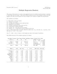
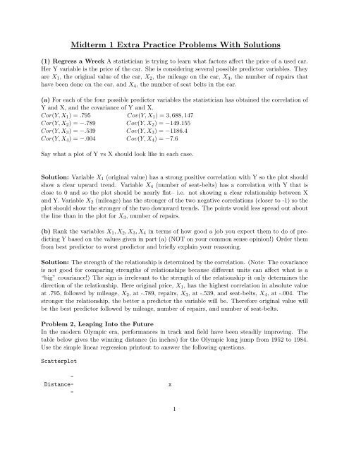
Midterm 1 Extra Practice Problems With Solutions(1) Regress a Wreck A statistician is trying to learn what factors affect the price of a used car.Her Y variable is the price of the car. She is considering several possible predictor variables. Theyare X 1 , the original value of the car, X 2 , the mileage on the car, X 3 , the number of repairs thathave been done on the car, and X 4 , the number of seat belts in the car.(a) For each of the four possible predictor variables the statistician has obtained the correlation ofY and X, and the covariance of Y and X.Cor(Y, X 1 ) = .795 Cov(Y, X 1 ) = 3, 688, 147Cor(Y, X 2 ) = −.789 Cov(Y, X 2 ) = −149.155Cor(Y, X 3 ) = −.539 Cov(Y, X 3 ) = −1186.4Cor(Y, X 4 ) = −.004 Cov(Y, X 4 ) = −7.6Say what a plot of Y vs X should look like in each case.Solution: Variable X 1 (original value) has a strong positive correlation with Y so the plot shouldshow a clear upward trend. Variable X 4 (number of seat-belts) has a correlation with Y that isclose to 0 and so the plot should be nearly flat– i.e. not showing a clear relationship between Xand Y. Variable X 2 (mileage) has the stronger of the two negative correlations (closer to -1) so theplot should show the stronger of the two downward trends. The points would less spread out aboutthe line than in the plot for X 3 , number of repairs.(b) Rank the variables X 1 , X 2 , X 3 , X 4 in terms of how good a job you expect them to do of predictingY based on the values given in part (a) (NOT on your common sense opinion!) Order themfrom best predictor to worst predictor and briefly explain your reasoning.Solution: The strength of the relationship is determined by the correlation. (Note: The covarianceis not good for comparing strengths of relationships because different units can affect what is a“big” covariance!) The sign is irrelevant to the strength of the relationship–it only determines thedirection of the relationship. Here original price, X 1 , has the highest correlation in absolute valueat .795, followed by mileage, X 2 , at -.789, repairs, X 3 , at -.539, and seat-belts, X 4 , at -.004. Thestronger the relationship, the better a predictor the variable will be. Therefore original value willbe the best predictor followed by mileage, number of repairs, and number of seat-belts.Problem 2, Leaping Into the FutureIn the modern Olympic era, performances in track and field have been steadily improving. Thetable below gives the winning distance (in inches) for the Olympic long jump from 1952 to 1984.Use the simple linear regression printout to answer the following questions.Scatterplot-Distance--x1

-340+- x x-- x- x320+ x- x-- x-300+ x----------+---------+---------+---------+---------+--------Year1956.0 1962.0 1968.0 1974.0 1980.0Regression AnalysisThe regression equation isDistance = - 1818 + 1.09 YearPredictor Coef StDev T PConstant -1817.8 706.1 -2.57 0.037Year 1.0885 0.3588 3.03 0.019Root MSE = 11.12 R-Sq = 56.8% R-Sq(adj) = 50.6%Analysis of VarianceSource DF SS MS F PRegression 1 1137.5 1137.5 9.21 0.019Residual Error 7 865.0 123.6Total 8 2002.5Unusual ObservationsObs Year Distance Fit StDev Fit Residual St Resid5 1968 350.50 324.42 3.71 26.08 2.49RR denotes an observation with a large standardized residual********************2

Year Distance1952 2981956 308.251960 319.751964 317.751968 350.51972 324.51976 328.51980 336.251984 336.25(a) Give the units and interpretation of b 1 in the simple regression model.Solution: The regression coefficient b 1 always gives than change in Y associated with a one unitchange in X. Since b 1 must convert from X units to Y units, the units of b 1 are the units of Ydivided by the units of X. In this problem, X is in years and Y is distance in inches, so the units ofb 1 are inches per year. Since b 1 = 1.08854, a one unit change in year is associated with a 1.08854inch change in distance, i.e. the winning long jump distance increases by 1.08854 inches per year.Naturally, since the Olympics are only held every four years, this really means that the winningdistance increases by about 4.35 inches every Olympiad.(b) According to this model what would have been the length of the winning jump if the Olympicshad been held in the year 1500. Does this make sense? Explain what has happened.Solution: According to this model the winning jump would have beenŶ = −1817.8 + 1.09(1500) = −182which obviously makes no sense at all! Models only work well in the range of the data used tobuild them. This model is based on the modern Olympics. The year 1500 is way way outside therange of our data. Perhaps there has been a rapid increase in long-jump distances in more recentyears because of improvements in technology, training techniques, nutrition, etc. that makes themodel now different from what it would have been in the past.Problem 3: Sneaker Sales You have just taken over the pricing department at Sneaky Zeke’sSneakers. Based on your wonderful education at UCLA you suspect that there is a relationshipbetween the price you charge for a pair of sneakers and the number of pairs of sneakers you willsell. Looking over recent sales records you see that stores have sold your sneakers at a variety ofdifferent prices. Let X be the price that has been charged for a pair of sneakers (in dollars) and letY be the number of pairs that have been sold by a store in a given month. You have obtained dataon X and Y for n=12 months. Some useful quantities have also been computed for you. Use themto answer the following questions.3

¯X 100 Ȳ 100n 12 SSX 1200SCP -1200∑SSR 1200SSE 300 Xi 1200∑ X2i 121200∑Yi 1200∑ Y2i 121500∑Xi Y i 118800(a) Find the estimated regression coefficients, b 0 and b 1 . Show your work.Solution: We know thatandb 1 = SCPSSX = −12001200 = −1b 0 = Ȳ − b 1 ¯X = 100 − (−1)(100) = 200You could calculate SCP and SSX from scratch from the numbers given but there was no point indoing so.(b) Give the units and real-world interpretations of b 0 and b 1 . (If you couldn’t answer part (a),assume b 0 = 200 and b 1 = −1.8).Solution: The intercept, b 0 is the average value of Y when X=0 and is always in the same unitsas Y. Here we have b 0 = 200 which means that when sneakers cost $0 per pair (i.e. we give themaway) we will sell 200 pairs per month. The units are sneakers or number of pairs per month orsomething equivalent. Note that this answer doesn’t make much real-world sense since if you weregiving away free sneakers you could “sell” an arbitrarily high number–and you are NOT likely tocharge $0 per pair!The slope, b 1 , gives the average change in Y associated with a one unit change in X, and its unitsare the units of Y divided by the units of X. Here b 1 = 1 so for each $1 extra we charge per pair ofsneakers we sell 1 fewer pairs per month on average. The units are pairs per dollar per month.(c) Recall that the correlation, ˆρ, gives the strength and direction of the relationship between Yand X. It turns out that ˆρ 2 = R 2 , the percentage of variability in Y that is explained by X in aregression model. Suppose that in this model X explains 80% or .8 of the variation in Y. Use thisfact to find the correlation between price and number of pairs of sneakers sold. Briefly explain anychoices that you make while doing this calculation.Solution: We are told that when you square the correlation you get R 2 for a regression. Thus toget the correlation all we have to do is take the square root of R 2 . The only thing you have to becareful about is the sign. Here we know from previous parts that there is a negative relationshipbetween price and sales so we must take the negative square root. The answer isˆρ = − √ .80 = −.89444

(d) Predict the number of pairs of sneakers that will be sold in a month if you charge a price of$300 per pair. Does this answer make real-world sense? Explain. What do you think might havecaused this result?Solution: To get the prediction all we have to do is plug X = 300 into the regression equation.We find that at a price of $300 per pair we sell on averageŶ = 200 − 1(300) = −100pairs of sneakers. Obviously this does not make real world sense–you can’t sell negative pairs ofsneakers! Probably the prediction is bad because we are projecting way outside the range of ourdata. We know that an average price for these sneakers was $100 so $300 is pretty extreme.(e) In part (a) you found that the estimated regression equation for predicting Y, the number ofpairs of sneakers sold in a month, using X, the price of a pair of sneakers. Use this informationto write down the equation for predicting TOTAL SALES IN DOLLARS FOR A MONTH. Hint:Think about the relationship between total sales in dollars, number of items sold, and price. (Note:If you couldn’t do part (a), you may assume b 0 = 200 and b 1 = −1.8.)Solution: The hint is the key to this problem. Total sales (TS) in dollars is equal to the numberof pairs sold (Y = b 0 + b 1 X) multipled by the sale price (X). Thus we haveT S = (200 − X)(X) = 200X − X 2(f)(Optional Bonus) Using your answer to part (e) figure out the optimal price for the companyto charge for their product to maximize sales. (Hint: The expression aX 2 + bX + c is maximizedby setting X = −b/2a.)Solution: Based on the answer to part (g) we want to maximize −1X 2 + 200X + 0 which will beachieved at the value−(200)2(−1) = −200−2 = 100Thus the optimal price is $100. Note that you could derive this answer using calculus by differentiatingthe equation for total sales and setting it equal to 0. I didn’t expect you to be able to dothis necessarily so I gave you the hint formula.Problem 4: Quickie Quiz Let Y be your score on a midterm (out of 100 points), let X 1 be thenumber of hours you study for the midterm, and let X 2 be the number of class sessions you skippedbefore the midterm. Suppose you fit simple linear regressions of your midterm score on each ofthese variables and findŶ = 20 + 5X 1 and Ŷ = 90 − 10X 2Say whether each of the following statements is True or False. If the answer is false, brieflyexplain why. If the statement is true you do not need to explain your reasoning although doing so5

may help you get partial credit if you are wrong.(a) The average score of people who didn’t study for the exam was about 20.Solution: This is TRUE–the intercept of the equation for X 1 is b 0 = 20 and it represents theaverage value of Y when X 1 = 0 hours are spent studying.(b) The slope estimate b 1 = −10 in the regression of midterm score on number of classes skippedmeans that every class you skip causes your midterm score to go down by 10 points on average.Solution: This is FALSE. The existence of a relationship does not prove cause. (“Correlation isnot causation.”) Putting the word cause in bold face was supposed to be a hint. What we cansay is that skipping an additional class is associated with an average drop in score of 10 points.In this instance there may well be a causal relationship–at least if the professor is any good–butwe can’t prove it with the regression model. Also, there are probably other factors that affect testscore such as how bright you are, how much you study, and whether you make up the material youmissed. It could be that the people who skip class are also the people who don’t care and don’tstudy very much and that this is the real cause of their poor performance.(c) The fact that the coefficient of X 1 is positive and the coefficient of X 2 is negative means thathours studied is a better predictor of midterm score than number of classes skipped.Solution: This is FALSE. The sign of the regression coefficient only gives the direction, not thestrength of the relationship. A positive sign means there is a positive relationship between studyingand exam score. The negative sign means there is a negative relationship between exam score andskipping class. Both of these relationships are probably strong. Most answers stopped at this pointand we were pretty lenient. However, to be complete you really ought to explain WHY the sign tellsyou nothing about the strength of the relationship. There are many ways to do this. For instanceyou could give an example of a perfect negative relationship to show that negative relationshipscan be very strong.(d) (Optional Bonus–no credit given without explanation) The fact that b 1 = 5 in theequation for studying is smaller in absolute value than b 1 = −10 in the equation for classes skippedmeans that the relationship between midterm score and studying is weaker than the relationshipbetween midterm score and skipping class.This is FALSE. The reason is that the two X variables are in completely different units so theircoefficients are not at all comparable.Problem 5: Race and Politics During the recent election between the blue party and the redparty, race was a major issue. Now that it is over, the blue party has conducted a poll to see howthey were fared with different ethnic groups. They surveyed n=400 voters and recorded their age(in years), their income (in thousands of dollars), their ethnicity: white (W), black (B), asian (A),or hispanic (H), and who they voted for: the blue candidate (BL), or the red candidate (RD).6

(a) The blue party statistician suspects that which party people voted for may depend their ethnicity.(In particular, historical precedent suggests that minorities tend to favor the blue party.)To check this she has conducted a contingency table analysis. The STATA printout is given below.State the null and alternative hypotheses she is testing, give the p-value and test statistic, andexplain your real-world conclusions. Based on the printout, explain briefly which groups of peopleappear to prefer the blue party more than the public as a whole and which groups the blue partyneeds to make more effort to reach out to.. tabi 40 60\ 60 40\47 53\ 40 60, chi2 exp+--------------------+| Key ||--------------------|| frequency || expected frequency |+--------------------+| colrow | Blue Red | Total-----------+----------------------+----------White | 40 60 | 100| 46.8 53.3 | 100.0-----------+----------------------+----------Black | 60 40 | 100| 46.8 53.3 | 100.0-----------+----------------------+----------Hispanic | 47 53 | 100| 46.8 53.3 | 100.0-----------+----------------------+----------Asian | 40 60 | 100| 46.8 53.3 | 100.0-----------+----------------------+----------Total | 187 213 | 400| 187.0 213.0 | 400.0Pearson chi2(3) = 10.7153 Pr = 0.013Solution: Now we are asked to perform a chi-squared test of independence. Our hypotheses, asalways for such a test, areH 0 : There is no relationship between ethnicity and voting choice–the two variables are independentH A : There is a relationship between ethnicity and who the person voted for.7

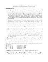
Note that I do not state the hypotheses here mathematically because this is a bit messy. Rememberthat in a contingency table problem, the hypotheses are really about the proportions of peoplewho fall in each category–and we have many categories here. You coudl in fact say that the nullhypothesis is that the proportion of each ethnic group that votes for the blue party was the same:p W = p B = p H = p A .Our test statistic is χ 2 = 10.715 and the corresponding p-value is .013 which is less than ourα = .05. We therefore reject the null hypothesis and conclude that there is a relationship betweena person’s ethnicity and which party they voted for. To determine which groups favored the blueparty more than the public as a whole we need compare the actual votes to what would havebeen expected under the assumption of no relationship. We see from the expected counts that inthe population as a whole 46.75% of people voted for the blue party. Thus Blacks at 60% andHispanics at 47% favored the blue part more than the population as a whole did, although in thelatter case it was very close. Whites and Asians voted for the blue party less than the populationas a whole. These are the two groups that the blue party needs to improve with most, althoughthey may also want to work on Hispanics since even that group did not give them a 50% majority..(b) Would it have been more appropriate to use Fisher’s exact test for this problem? Explain briefly.Solution: Since the expected counts in the table are all well above 5 (and indeed all the samplesizes and observed counts are large 2) the normal approximation will be very accurate–it is notnecessary to use Fisher’s exact test. In fact, we only learned how to do Fisher’s exact test for a 2by 2 contingency table so I wouldn’t have expected you to be able to do it here anyway!(c) Based on the results of part (a), the national chair of the blue party claims that people votefor one candidate or the other because of their ethnicity. Is this claim correct? If so, explain why.If not, explain why not and give an example of why it might be wrong based on your available data.Solution: This claim is wrong! Correlation is not causation. Just because people from differentethnic groups voted differently does not mean it was their ethnicity that caused them to do so.Perhaps people of different ethnicity have different incomes on average and their votes were determinedby their income rather than their ethnicity. Note that to get full credit you needed to supplya possible alternative factor that could be related to both ethnicity and voting choice. It was notenough to just say correlation is not causation.Problem 6: Rudolph the Red Nosed Statistics Student Poor Rudolph! His nose is red fromsneezing with the flu while staying up all night studying for his statistics final. While procrastinatinghe has come across an interesting article about flu treatments. A medical center has conducteda study of 250 people. 50 were randomly chosen to receive a placebo, 100 were given the standardflu vaccine, and 100 were given the new nasal spray flu “vaccine.” The organizers of the studyrecorded in each case the type of treatment received, the age of the subject, and whether or notthe subject ultimately got the flu. A STATA contingency table analysis for the treatment and fluvariables is shown below.. tabi 15 28 15\ 35 72 85, chi2 exp8

+--------------------+| Key ||--------------------|| frequency || expected frequency |+--------------------+| colrow | Placebo Vaccine Spray | Total-----------+---------------------------------+----------Flu | 15 28 15 | 58| 11.6 23.2 23.2 | 58.0-----------+---------------------------------+----------No Flu | 35 72 85 | 192| 38.4 76.8 76.8 | 192.0-----------+---------------------------------+----------Total | 50 100 100 | 250| 50.0 100.0 100.0 | 250.0Pearson chi2(2) = 6.3645 Pr = 0.041(a) State in words the null and alternative hypotheses that are being tested by the contingencytable analysis and give your real-world conclusions. Which one (if any) of the three treatmentsseems to be the most effective? Briefly justify your answers.Solution: In contingency table problems we always test a null hypothesis of no relationship versusan alternative of a relationship. Specifically in the context of this problem we haveH 0 : There is no relationship between WHICH treatment you got and WHETHER or not you gotthe flu.H A : There is a relationship between WHICH treatment you got and WHETHER or not you gotthe flu.Note that my hypotheses do not specify which treatment is better–they just say whether or notthere is a relationship! Since the p-value for the chi-squared test is .041 which is less than myα = .05 I reject the null hypothesis and conclude that how likely you are to get the flu does dependon which of the three treatments you got. From the table it looks as if the spray vaccine groupis doing the best. Only 15/100 = 15% of that group got the flu compared to 30% for the placeboand 28% for the standard vaccine. Alternatively you could note that the spray group has fewer flucases (15) than expected (23.2) while the other two groups have more flu cases than expected.(b) The organizers of the study would like to claim that taking the nasal flu treatment causes yourchances of getting the flu to go down. Can they say this? Why or why not.Solution: This is TRUE. Normally correlation is not causation. However, since this is an exper-9

imental study where people have been randomized to different treatments we have eliminated allthe other factors that could be causing differences between the groups. The only difference is whattreatment people got so we have actually proved that the new nasal spray vaccine is better thannothing (placebo) or the standard treatment.10