Annotated Multiple Regression Example - UCLA Biostatistics

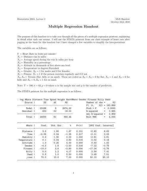
arbitrary. We are told that the gender variable, X 6 = 1 for males and X 6 = 0 for females. For an indicatorvariable it does not really make sense to talk about a slope. You can’t have a “1 unit change in gender.”What you can do is talk about the difference between males and females. With an indicator variable, thecoefficient tells you the average difference in Y between people who have the characteristic (X = 1) and thosewho do not (X = 0). For gender in this model we have b 6 = −4 meaning all else equal (same distance andtime run, humidity, temperature, altitude, fitness and terrain), a man (X 6 = 1) will have a heart rate that is4 beats per minute slower (the negative sign) than a woman (X 6 = 0). The confidence interval of [-7.22, -.78]says we are 95% sure that on average a man has an exercising heart rate somewhere between .78 and 7.22beats per minute slower than an otherwise equivalent woman. Since the entire interval is below 0, we areconfident that the men do indeed have the slower heart rates on average. Similarly, the coefficient b 7 = −10means that a person who exercises regularly will have a heart rate on average 10 beats per minute slowerafter exercise than a person who does not exercise regularly will have under the same conditions. Onceagain the entire interval is below 0, meaning that all else equal, regular exercise is associated with a lowerexercising heart rate with the amount of the decrease being anywhere from 17.24 to 2.76 beats per minutefrom the confidence interval. The last measure of interest in this model is the terrain on which the race wasrun. We have three categories of terrain: flat, hilly and sandy. When you have a qualitative variable withmore than 2 categories you use multiple indicators to describe it. One group serves as the reference andhas all the indicators equal to 0 and the other categories are compared to that reference. Here flat terrain,X 8 = X 9 = 0 is the reference category and hilly (X 8 = 1, X 9 = 0) and sandy (X 8 = 0, X 9 = 1) are comparedto it with the coefficients of X 8 and X 9 giving the respective differences. Specifically, b 8 = 5.0 means allelse equal, a person running on flat terrain will have an exercising heart rate 5 beats per minute higher thansomeone running on flat terrain, while b 9 = 5.5 means someone running on sandy terrain will have a heartrate of 5.5 beats per minute higehr than someone who does a comparable run on flat terrain. Of course wecan deduce from this that someone running on sand will on average have a heart rate .5 beats per minutefaster than someone running on hilly terrain. The corresponding confidence intervals give the possible rangesfor these differences. Note that the CIs for β 8 and β 9 overlap quite a bit meaning that running on hilly orsandy terrain may have an equal impact on heart rate compared to flat terrain–in other words those twosurfaces may not be significantly different from each other, although to be sure we would need to test thatdirectly.Measuring Model PerformanceAs in simple linear regression, to evaluate how good a job the model is doing we divide the total variabilityin Y into a piece that can be attributed to our X variables and a piece that can not. Here that amountsto saying that some of the differences in exercising heart rate can be attributed to distance and time run,atmospheric conditions such as humidity and termperature, geographical conditions such as altitude andtype of terrain, and to personal characteristics including gender and basic fitness. However there may beother factors which we have not included that will cause a model based on these variables not to makeperfect predictions. This division of the variability into two components results in an ANOVA table whichin turn provides our usual measures for comparing regression models, R 2 , Radj 2 and RMSE. These values canbe interpreted as follows.SST: The “Sum of Squares Total” is a measure of the total variability in Y and is just the variance in Ywithout dividing by n-1. It serves as our reference point for deciding how well a regression model is fitting.You can think if it as the total (squared) error we would make in predicting the Y values in our sampleif we ignored the information in our X variables and just always guessed Ȳ . The raw number is hard tointerpret as anything other than a reference point, especially as it gets bigger as the sample size increases.Here SST = 24,000 is the total variability in the exercising heart rates of the people in our jogging sample.Some if it is due to the 9 predictor variables and some of it is due to other factors that we did not measure.3

RMSE = MSE/(n-p-1): This number is called “root mean squared error” and tells you the average errorper data point that you make when you use all the X’s to predict Y. Here RMSE = 4.0 means that on averagewhen we predict a person’s exercising heart rate using distance, time, humidity, temperature, altitude,gender, fitness and terrain we are typically off by about 4 beats per minute. We were told that the averageexercising heart rate for people in this data set was Ȳ = 100 so our average error is about 4%. The modelseems to make quite accurate predictions. Note that you don’t have to compare to Ȳ specifically–sometimesit is useful to look at the minimum and maximum Y to get an idea of best-case/worst-case scenarios forinstance–but it is critical to use the context of the problem to determine how good the predictions are.F: F = MSR/MSE is the ratio of explained to unexplained variability. The bigger it is, the better a job themodel as a whole is doing and the more sure we wuill be that there is a statistically significant relationshipbetween Y and at least one of the X variables. On an intuitive level, F = 1 represents a balance betweenexplained an unexplained variability so we are looking for values much bigger than 1. To really fell whetheryour F statistic is big you look at the corresponding p-value (Prob > F) on the STATA printout). A smallp-value means your F counts as big (see below for details). Here our F = 160.889 which is much bigger than1 and the corresponding p-value of 0 is very small so it looks like the model as explained much more of thevariability in heart rates than it hasn’t explained. We can make this into a more formal test if we make someassumptions.Inference In Multiple RegressionThe summary measures above derive naturally from the least squares formulation of teh regresison line anddo not implicitly make any assumptions about the distributions of the various pieces of the model. However,if we do make some assumptions we can actually obtain confidence intervals for the various model parameters,and also perform hypothesis tests about the model as a whole and the contributions of the individualvariables. Specifically we assume that the error terms on our model are independent, normally distributed,mean 0 and have constant variance for all values of X. Under these assumptions the least squares estimatesb 0 , b 1 , . . . , b p , MSE are unbiased estimates of β 0 , β 1 , . . . , β p , σ 2 and the esitmated slope and intercept arenormally distributed with standard errors we can compute using matrix algebra. From this we can get thefollowing forms of inference.Overall F test: The first thing we would like to determine is whether the model as a whole is useful. Recallthat our multiple linear regression model isY = β 0 + β 1 X 1 + · · · β p X p + ɛIf all the β’s are 0 then none of the X’s will make a contribution to predicting Y and the model will not beuseful. We therefore want to test (in the context of the current example):H 0 : β 1 = β 2 = · · · = β 9 = 0–none of distance, time, humidity, temperature, altitude, gender, fitness orterrain helps to explain exercising heart rate. The model as a whole is not useful.H A : At least one of β 1 , . . . , β 9 ≠ 0–at least one of distance, time, etc. IS useful for explaining heart rateafter jogging. The model as a whole IS useful.As discussed above, a reasonable test statistic for looking at this set of hypotheses is F obs = MSR/MSE.The bigger this is, the more of the variability in heart rates in our sample has been explained by the predictorsand the more convinced we are that the model as a whole is useful. Here we have F = 160.889. Under the nullhypothesis, F obs has an F distribution with p and n-p-1 degrees of freedom and the corresponding p-value isP (F 9,52 ≥ 160.889) = 0.00005

so we reject the null hypothesis and conclude (not surprisingly!) that at least one of these 9 factors doeshave something to do with heart rate. Of course this test does not tell us WHICH variable or variables isuseful. For that we need the following.Individual t-tests: To determine whether a variable makes a useful contribution to a multiple regressionmodel you use a t-test. Note that this test does NOT ask whether the variable by itself is related to Y. Itinstead asks whether the variable in question provides any information about Y that was not providedby the other variables in the model. Since your predictor variables can be related to each other it isquite possible that some of them provide the same information about Y and that as a result a variable thatby itself is related to Y may not be significant as part of the larger model. Formally the hypotheses work asfollows. I use X 1 , the distance variable, as an example in this model. The others work similarly:H 0 : β 1 = 0–after accounting for time run, humidity, temperature, altitude, gender, fitness and terrain,knowing the distance a person has run does not provide any additional information about exercising heartrate. X 1 is not worth adding to a model tha already contains these other factors.H A : β 1 ≠ 0–distance run provides additional information about heart rate beyond what is explained bytime, humidity, etc. It is worth adding to the model.Our test statistic ist obs = b 1 − 0s b1= 1.67Under the null hypothesis t obs has a t distribution with n-p-1 and the two-sided p-value (which is what isgive on the STATA regression printout next to the t statistic) isp − value = 2P (t 52 ≥ 1.67) = .101Since this p-value os greater than α = .05 we fail to reject the null hypothesis. We do not have sufficientevidence to conclude that the distance run provides additional infromation about heart rate than what isexplained by the other 8 variables. It may not be a useful addition to this model.Of the 9 variables in the current model, all except distance, time and humidity appear to be significantwith p-values < .05. However we can’t simply decide to remove these variables from the model all at oncebecause their p-values depend on the presence of ALL the other variables. For instance it is quite possiblethat distance and time of the run are providing the same information and if we removed one of them theother would be significant.Confidence Intervals for β j ′ s: The STATA printout also gives confidence intervals for the intercept andeach of the slopes in the regression model. These are in the last column of the parameter estimates table.If they were not given we could get them from the parameter estimates themselves and their standarderrors which are given in the columns labeled “Coef.” for coefficients and “STd. Err.” for standard error.Specifically a confidence interval for a β in a regresison model is given byb j ± t α/2,n−p−1 s bjHere for a 95% confidence interval we would need t .025,52 = 2.01 so the confidence interval for β 1 for instanceis3.0 ± 2.01(1.8) = [−.62, 6.62]The other intervals are obtained analagously and their interpretations have been given above along with theinterpretations of the intercept and slopes.6