Using MODIS 250 m Imagery to Estimate Total Suspended Sediment

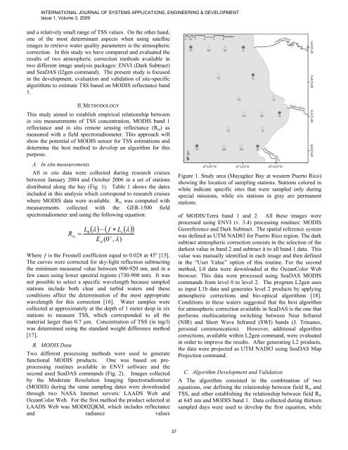
INTERNATIONAL JOURNAL OF SYSTEMS APPLICATIONS, ENGINEERING & DEVELOPMENTIssue 1, Volume 3, 2009and a relatively small range of TSS values. On the other hand,one of the most determinant aspects when using satelliteimages to retrieve water quality parameters is the atmosphericcorrection. In this study we have compared and evaluated theresults of two atmospheric correction methods available intwo different image analysis packages: ENVI (Dark Subtract)and SeaDAS (l2gen command). The present study is focusedin the development, evaluation and validation of site-specificalgorithms to estimate TSS based on MODIS reflectance band1.II. METHODOLOGYThis study aimed to establish empirical relationship betweenin situ measurements of TSS concentration, MODIS band 1reflectance and in situ remote sensing reflectance (R rs ) asmeasured with a field spectroradiometer. This approach willshow the potential of MODIS sensor for TSS estimations anddetermine the best method to develop an algorithm for thispurpose.A. In situ measurementsAll in situ data were collected during research cruisesbetween January 2004 and October 2006 in a set of stationsdistributed along the bay (Fig. 1). Table 1 shows the datesincluded in this analysis which correspond to research cruiseswhere MODIS data were available. R rs was computed withmeasurements collected with the GER-1500 fieldspectroradiometer and using the following equation:RrsL=0( λ) − ( f ∗ L ( λ))ds+E (0 , λ)Where ƒ is the Fresnell coefficient equal to 0.028 at 45 o [15].The curves were corrected for sky-light reflection subtractingthe minimum measured value between 900-920 nm, and in afew cases using lower spectral regions (730-900 nm). It wasnot possible to select a specific wavelength because sampledstations include both clear and turbid waters and theseconditions affect the determination of the most appropriatewavelength for this correction [16]. Water samples werecollected at approximately at the depth of 1 meter deep in sixstations to measure TSS, which corresponded to all thematerial larger than 0.7 μm. Concentration of TSS (in mg/l)was determined using the standard weight difference method[17].B. MODIS DataTwo different processing methods were used to generatefunctional MODIS products. One was based on preprocessingroutines available in ENVI software and thesecond used SeaDAS commands (Fig. 2). Images collectedby the Moderate Resolution Imaging Spectroradiometer(MODIS) during the same sampling dates were downloadedthrough two NASA Internet servers: LAADS Web andOceanColor Web. For the first method the product selected atLAADS Web was MOD02QKM, which includes reflectanceand radiance valuesFigure 1. Study area (Mayagüez Bay at western Puerto Rico)showing the location of sampling stations. Stations colored inwhite indicate specific sites that were sampled only duringspecial missions, while six stations in gray are permanentstations.of MODIS/Terra band 1 and 2. All these images wereprocessed using ENVI (v. 3.4) processing routines: MODISGeoreference and Dark Subtract. The spatial reference systemwas defined as UTM NAD83 for Puerto Rico region. The darksubtract atmospheric correction consists in the selection of thedarkest value in band 2 and subtract it to all band 1 data. Thisvalue was manually identified in each image and then definedin the “User Value” option of this routine. For the secondmethod, L0 data were downloaded at the OceanColor Webbrowser. This data were processed using SeaDAS MODIScommands from level 0 to level 2. The program L2gen usesas input L1b data and generates level 2 products by applyingatmospheric corrections and bio-optical algorithms [18].Conditions in these waters suggested that the best algorithmfor atmospheric correction available in SeaDAS is the one thatperforms multiscattering switching between Near Infrared(NIR) and Short Wave Infrared (SWI) bands (J. Trinanes,personal communication). However, additional algorithmcorrections, available within L2gen command, were evaluatedin order to improve the results. After generating L2 products,the data were projected as UTM NAD83 using SeaDAS MapProjection command.C. Algorithm Development and ValidationA The algorithm consisted in the combination of twoequations, one defining the relationship between field R rs andTSS, and other establishing the relationship between field R rsat 645 nm and MODIS band 1. Data collected during thirteensampled days were used to develop the first equation, while37