- Page 1 and 2:
Jim Hefferonhttp://joshua.smcvt.edu
- Page 3 and 4:
PrefaceThis book helps students to
- Page 5 and 6:
If you are reading this on your own
- Page 7 and 8:
ContentsChapter One: Linear Systems
- Page 9:
Chapter Five: SimilarityI Complex V
- Page 12 and 13:
2 Chapter One. Linear Systemsmust e
- Page 14 and 15:
4 Chapter One. Linear SystemsEach o
- Page 16 and 17:
6 Chapter One. Linear Systems(Had t
- Page 18 and 19:
8 Chapter One. Linear Systemsany so
- Page 20 and 21:
10 Chapter One. Linear Systems(b) C
- Page 22 and 23:
12 Chapter One. Linear SystemsCompa
- Page 24 and 25:
14 Chapter One. Linear SystemsMatri
- Page 26 and 27:
16 Chapter One. Linear Systems2.12
- Page 28 and 29:
18 Chapter One. Linear Systemsthe g
- Page 30 and 31:
20 Chapter One. Linear Systems(b) a
- Page 32 and 33:
22 Chapter One. Linear SystemsStudy
- Page 34 and 35:
24 Chapter One. Linear Systemsleadi
- Page 36 and 37:
26 Chapter One. Linear SystemsThat
- Page 38 and 39:
28 Chapter One. Linear SystemsWe ha
- Page 40 and 41:
30 Chapter One. Linear Systemš 3.
- Page 42 and 43:
32 Chapter One. Linear SystemsIILin
- Page 44 and 45:
34 Chapter One. Linear Systemsvecto
- Page 46 and 47:
36 Chapter One. Linear Systemsand l
- Page 48 and 49:
38 Chapter One. Linear Systems(b) t
- Page 50 and 51:
40 Chapter One. Linear Systemsis th
- Page 52 and 53:
42 Chapter One. Linear Systems2.6 C
- Page 54 and 55:
44 Chapter One. Linear Systems(b) S
- Page 56 and 57:
46 Chapter One. Linear SystemsIIIRe
- Page 58 and 59:
48 Chapter One. Linear Systems1.4 E
- Page 60 and 61:
50 Chapter One. Linear SystemsExerc
- Page 62 and 63:
52 Chapter One. Linear Systems2.3 L
- Page 64 and 65:
54 Chapter One. Linear SystemsBy th
- Page 66 and 67:
56 Chapter One. Linear SystemsThe u
- Page 68 and 69:
58 Chapter One. Linear Systems2.22
- Page 70 and 71:
60 Chapter One. Linear Systems7 2 5
- Page 72 and 73:
62 Chapter One. Linear Systemsestim
- Page 74 and 75:
64 Chapter One. Linear Systems3 Thi
- Page 76 and 77:
66 Chapter One. Linear Systemscompu
- Page 78 and 79:
68 Chapter One. Linear Systemsworke
- Page 80 and 81:
70 Chapter One. Linear SystemsCompo
- Page 82 and 83:
72 Chapter One. Linear SystemsKirch
- Page 84 and 85:
74 Chapter One. Linear Systems(b) L
- Page 86 and 87:
76 Chapter Two. Vector SpacesIDefin
- Page 88 and 89:
78 Chapter Two. Vector SpacesThe ni
- Page 90 and 91:
80 Chapter Two. Vector Spaces1.7 De
- Page 92 and 93:
82 Chapter Two. Vector Spaces1.13 E
- Page 94 and 95:
84 Chapter Two. Vector SpacesLinear
- Page 96 and 97:
86 Chapter Two. Vector Spaces1.32 P
- Page 98 and 99:
88 Chapter Two. Vector Spacesand sc
- Page 100 and 101:
90 Chapter Two. Vector Spacescombin
- Page 102 and 103:
92 Chapter Two. Vector Spaces2.17 E
- Page 104 and 105:
94 Chapter Two. Vector Spaceš 2.2
- Page 106 and 107:
96 Chapter Two. Vector Spaces(b) Wh
- Page 108 and 109:
98 Chapter Two. Vector Spaces1.2 De
- Page 110 and 111:
100 Chapter Two. Vector Spaces1.9 E
- Page 112 and 113:
102 Chapter Two. Vector Spaces1.13
- Page 114 and 115:
104 Chapter Two. Vector SpacesThus
- Page 116 and 117:
106 Chapter Two. Vector Spaceš 1.
- Page 118 and 119:
108 Chapter Two. Vector Spaceslinea
- Page 120 and 121:
110 Chapter Two. Vector SpacesThe v
- Page 122 and 123:
112 Chapter Two. Vector Spacesholds
- Page 124 and 125:
114 Chapter Two. Vector Spaces1.18
- Page 126 and 127:
116 Chapter Two. Vector Spaces2.2 R
- Page 128 and 129:
118 Chapter Two. Vector Spaces2.10
- Page 130 and 131:
120 Chapter Two. Vector Spaceš 2.
- Page 132 and 133:
122 Chapter Two. Vector Spaces3.4 L
- Page 134 and 135:
124 Chapter Two. Vector SpacesThe c
- Page 136 and 137:
126 Chapter Two. Vector SpacesProof
- Page 138 and 139:
128 Chapter Two. Vector Spaces(c) P
- Page 140 and 141:
130 Chapter Two. Vector Spacesthe y
- Page 142 and 143:
132 Chapter Two. Vector SpacesFinal
- Page 144 and 145:
134 Chapter Two. Vector SpacesIn th
- Page 146 and 147:
136 Chapter Two. Vector Spaces4.41
- Page 148 and 149:
138 Chapter Two. Vector Spacesusual
- Page 150 and 151:
140 Chapter Two. Vector Spacestake
- Page 152 and 153:
142 Chapter Two. Vector Spaces(c) F
- Page 154 and 155:
144 Chapter Two. Vector SpacesThe i
- Page 156 and 157:
146 Chapter Two. Vector Spacesdirec
- Page 158 and 159:
148 Chapter Two. Vector Spaces(d) C
- Page 160 and 161:
150 Chapter Two. Vector Spaceswill
- Page 162 and 163:
152 Chapter Two. Vector SpacesThe s
- Page 164 and 165:
154 Chapter Two. Vector SpacesThere
- Page 166 and 167:
156 Chapter Two. Vector Spaces
- Page 168 and 169:
158 Chapter Three. Maps Between Spa
- Page 170 and 171:
160 Chapter Three. Maps Between Spa
- Page 172 and 173:
162 Chapter Three. Maps Between Spa
- Page 174 and 175:
164 Chapter Three. Maps Between Spa
- Page 176 and 177:
166 Chapter Three. Maps Between Spa
- Page 178 and 179:
168 Chapter Three. Maps Between Spa
- Page 180 and 181:
170 Chapter Three. Maps Between Spa
- Page 182 and 183:
172 Chapter Three. Maps Between Spa
- Page 184 and 185:
174 Chapter Three. Maps Between Spa
- Page 186 and 187:
176 Chapter Three. Maps Between Spa
- Page 188 and 189:
178 Chapter Three. Maps Between Spa
- Page 190 and 191:
180 Chapter Three. Maps Between Spa
- Page 192 and 193:
182 Chapter Three. Maps Between Spa
- Page 194 and 195:
184 Chapter Three. Maps Between Spa
- Page 196 and 197:
186 Chapter Three. Maps Between Spa
- Page 198 and 199:
188 Chapter Three. Maps Between Spa
- Page 200 and 201:
190 Chapter Three. Maps Between Spa
- Page 202 and 203:
192 Chapter Three. Maps Between Spa
- Page 204 and 205:
194 Chapter Three. Maps Between Spa
- Page 206 and 207:
196 Chapter Three. Maps Between Spa
- Page 208 and 209:
198 Chapter Three. Maps Between Spa
- Page 210 and 211:
200 Chapter Three. Maps Between Spa
- Page 212 and 213:
202 Chapter Three. Maps Between Spa
- Page 214 and 215:
204 Chapter Three. Maps Between Spa
- Page 216 and 217:
206 Chapter Three. Maps Between Spa
- Page 218 and 219:
208 Chapter Three. Maps Between Spa
- Page 220 and 221:
210 Chapter Three. Maps Between Spa
- Page 222 and 223:
212 Chapter Three. Maps Between Spa
- Page 224 and 225:
214 Chapter Three. Maps Between Spa
- Page 226 and 227:
216 Chapter Three. Maps Between Spa
- Page 228 and 229: 218 Chapter Three. Maps Between Spa
- Page 230 and 231: 220 Chapter Three. Maps Between Spa
- Page 232 and 233: 222 Chapter Three. Maps Between Spa
- Page 234 and 235: 224 Chapter Three. Maps Between Spa
- Page 236 and 237: 226 Chapter Three. Maps Between Spa
- Page 238 and 239: 228 Chapter Three. Maps Between Spa
- Page 240 and 241: 230 Chapter Three. Maps Between Spa
- Page 242 and 243: 232 Chapter Three. Maps Between Spa
- Page 244 and 245: 234 Chapter Three. Maps Between Spa
- Page 246 and 247: 236 Chapter Three. Maps Between Spa
- Page 248 and 249: 238 Chapter Three. Maps Between Spa
- Page 250 and 251: 240 Chapter Three. Maps Between Spa
- Page 252 and 253: 242 Chapter Three. Maps Between Spa
- Page 254 and 255: 244 Chapter Three. Maps Between Spa
- Page 256 and 257: 246 Chapter Three. Maps Between Spa
- Page 258 and 259: 248 Chapter Three. Maps Between Spa
- Page 260 and 261: 250 Chapter Three. Maps Between Spa
- Page 262 and 263: 252 Chapter Three. Maps Between Spa
- Page 264 and 265: 254 Chapter Three. Maps Between Spa
- Page 266 and 267: 256 Chapter Three. Maps Between Spa
- Page 268 and 269: 258 Chapter Three. Maps Between Spa
- Page 270 and 271: 260 Chapter Three. Maps Between Spa
- Page 272 and 273: 262 Chapter Three. Maps Between Spa
- Page 274 and 275: 264 Chapter Three. Maps Between Spa
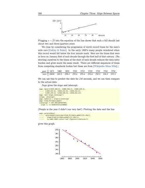
- Page 276 and 277: TopicLine of Best FitThis Topic req
- Page 280 and 281: 270 Chapter Three. Maps Between Spa
- Page 282 and 283: 272 Chapter Three. Maps Between Spa
- Page 284 and 285: 274 Chapter Three. Maps Between Spa
- Page 286 and 287: 276 Chapter Three. Maps Between Spa
- Page 288 and 289: 278 Chapter Three. Maps Between Spa
- Page 290 and 291: 280 Chapter Three. Maps Between Spa
- Page 292 and 293: TopicMarkov ChainsHere is a simple
- Page 294 and 295: 284 Chapter Three. Maps Between Spa
- Page 296 and 297: 286 Chapter Three. Maps Between Spa
- Page 298 and 299: TopicOrthonormal MatricesIn The Ele
- Page 300 and 301: 290 Chapter Three. Maps Between Spa
- Page 302 and 303: 292 Chapter Three. Maps Between Spa
- Page 304 and 305: 294 Chapter Three. Maps Between Spa
- Page 306 and 307: 296 Chapter Four. DeterminantsIDefi
- Page 308 and 309: 298 Chapter Four. Determinantsalso
- Page 310 and 311: 300 Chapter Four. Determinantš 1.
- Page 312 and 313: 302 Chapter Four. DeterminantsThe s
- Page 314 and 315: 304 Chapter Four. Determinants∣
- Page 316 and 317: 306 Chapter Four. Determinantsdeter
- Page 318 and 319: 308 Chapter Four. DeterminantsSo wi
- Page 320 and 321: 310 Chapter Four. Determinants3.10
- Page 322 and 323: 312 Chapter Four. Determinants3.20
- Page 324 and 325: 314 Chapter Four. Determinantsis: t
- Page 326 and 327: 316 Chapter Four. DeterminantsProof
- Page 328 and 329:
318 Chapter Four. DeterminantsFor p
- Page 330 and 331:
320 Chapter Four. DeterminantsIIGeo
- Page 332 and 333:
322 Chapter Four. DeterminantsThe s
- Page 334 and 335:
324 Chapter Four. Determinantš 1.
- Page 336 and 337:
326 Chapter Four. DeterminantsIIILa
- Page 338 and 339:
328 Chapter Four. DeterminantsAlter
- Page 340 and 341:
330 Chapter Four. Determinants⎛
- Page 342 and 343:
332 Chapter Four. DeterminantsThe s
- Page 344 and 345:
TopicSpeed of Calculating Determina
- Page 346 and 347:
336 Chapter Four. DeterminantsCount
- Page 348 and 349:
338 Chapter Four. DeterminantsLet C
- Page 350 and 351:
340 Chapter Four. Determinants3 The
- Page 352 and 353:
342 Chapter Four. DeterminantsIt is
- Page 354 and 355:
344 Chapter Four. DeterminantsPSIFo
- Page 356 and 357:
346 Chapter Four. Determinantsnonze
- Page 358 and 359:
348 Chapter Four. DeterminantsOT 1U
- Page 360 and 361:
350 Chapter Four. Determinantsthe c
- Page 362 and 363:
352 Chapter Four. Determinants(d) F
- Page 364 and 365:
354 Chapter Five. Similaritythe sca
- Page 366 and 367:
356 Chapter Five. SimilarityIn C we
- Page 368 and 369:
358 Chapter Five. SimilarityIISimil
- Page 370 and 371:
360 Chapter Five. Similarity(b) Fin
- Page 372 and 373:
362 Chapter Five. Similarity2.4 Lem
- Page 374 and 375:
364 Chapter Five. Similarity( ) ( )
- Page 376 and 377:
366 Chapter Five. Similaritythen 2
- Page 378 and 379:
368 Chapter Five. Similarity3.11 De
- Page 380 and 381:
370 Chapter Five. Similarity⃗0 =
- Page 382 and 383:
372 Chapter Five. Similarity3.43 Di
- Page 384 and 385:
374 Chapter Five. Similarityand thi
- Page 386 and 387:
376 Chapter Five. SimilarityThis gr
- Page 388 and 389:
378 Chapter Five. SimilarityThis is
- Page 390 and 391:
380 Chapter Five. SimilarityProof S
- Page 392 and 393:
382 Chapter Five. SimilarityProof F
- Page 394 and 395:
384 Chapter Five. Similarity2.17 Ex
- Page 396 and 397:
386 Chapter Five. Similarity̌ 2.26
- Page 398 and 399:
388 Chapter Five. Similaritywith re
- Page 400 and 401:
390 Chapter Five. Similaritycheck t
- Page 402 and 403:
392 Chapter Five. SimilarityWe refe
- Page 404 and 405:
394 Chapter Five. Similarity1.18 Wh
- Page 406 and 407:
396 Chapter Five. Similarityis (x
- Page 408 and 409:
398 Chapter Five. Similarity⃗m
- Page 410 and 411:
400 Chapter Five. Similarityeach te
- Page 412 and 413:
402 Chapter Five. Similarity2.14 Co
- Page 414 and 415:
404 Chapter Five. SimilaritySo the
- Page 416 and 417:
406 Chapter Five. Similarity(b) The
- Page 418 and 419:
TopicMethod of PowersIn application
- Page 420 and 421:
410 Chapter Five. SimilarityExercis
- Page 422 and 423:
TopicStable PopulationsImagine a re
- Page 424 and 425:
TopicPage RankingImagine that you a
- Page 426 and 427:
416 Chapter Five. SimilaritySo we r
- Page 428 and 429:
TopicLinear RecurrencesIn 1202 Leon
- Page 430 and 431:
420 Chapter Five. Similaritya n−k
- Page 432 and 433:
422 Chapter Five. Similarityof the
- Page 434 and 435:
424 Chapter Five. Similarity(b) f(n
- Page 436 and 437:
AppendixMathematics is made of argu
- Page 438 and 439:
A-3There are two main ways to estab
- Page 440 and 441:
A-5induction. Such a proof has two
- Page 442 and 443:
A-7Because of Extensionality, to pr
- Page 444 and 445:
A-9same role with respect to functi
- Page 446:
A-11S −1 = {. . . , −3, −1, 1
- Page 449 and 450:
[Arrow] Kenneth J. Arrow, Social Ch
- Page 451 and 452:
[Giordano, Jaye, Weir] Frank R. Gio
- Page 453 and 454:
[Quine] W. V. Quine, Methods of Log
- Page 455 and 456:
Indexaccuracyof Gauss’s Method, 6
- Page 457 and 458:
Euclid, 288even functions, 94, 134e
- Page 459 and 460:
Google, 416identity, 219, 223incide
- Page 461 and 462:
of a matrix, 193of a vector, 112rep
- Page 463:
spin, 145well-defined, A-8Wheatston