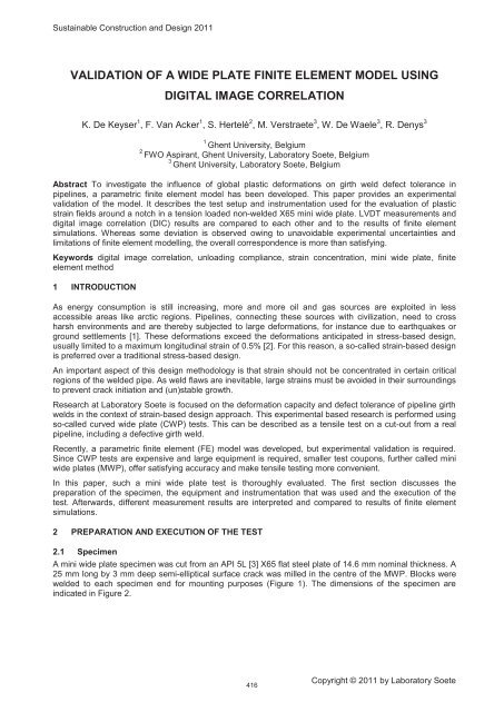
validation of a wide plate finite element model using digital image ...

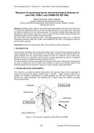
Sustainable Construction and Design 2011Figure 1: Test specimen with mounting blocks2.2 MaterialThe stress-strain relation (average of 6 tensile tests) of the pipeline steel in the longitudinal direction isshown in Figure 3. The plate material exhibits discontinuous yielding behaviour with a pronounced Lüdersplateau. The main tensile characteristics are listed in Table 1. Note that the yield-to-tensile stress ratio (Y/Tratio)is defined as the ratio between 0.2% proof stress R p0.2 and ultimate tensile stress R m .Table 1: Mechanical properties of API 5L X65 pipeline steelupper yield point R e 455.0MPa ultimate tensile stress R m 537.4 MPaproof stress R p0.2 433.5 MPa uniform elongation e m 16.1%0.5% strain offset R t0.5 433.5 MPa yield-to-tensile ratio R p0.2 /R m 0.83Lüders elongation e Lüders 2.62%Figure 2: Geometry and mounting positions ofmeasurement devices (figure not to scale)Figure 3: Longitudinal stress-strain curve of thematerialFor optical strain measurements, a randomly distributed speckle pattern was applied on the notched side ofthe specimen. The speckle pattern was obtained from a uniform layer of white spraying paint covered withspots of black lacquer paint. This pattern allows the Digital Image Correlation (DIC) camera system to trackdifferent regions of the MWP during the experiment. More information on this system is given in section2.3.3. To avoid crumbling of the paint layer during the test, the corrosion layer on the specimen wasremoved in advance.2.3 Test rig and measurement equipment2.3.1 MTS test rigA servo-hydraulic MTS universal test rig was used for this experiment. The system can exert a maximumforce of 2500 kN and a maximum piston displacement of 150mm.417Copyright © 2011 by Laboratory Soete

Sustainable Construction and Design 20112.3.2 LVDTs and clip gaugeTo measure the deformation at different locations of the specimen, 4 LVDTs were mounted on the backsideof the specimen according to the UGent guidelines for CWP testing [4]. Two of them with gauge length 108mm (K1 and K2) were located in the gross section of the specimen, away from the notch. The two otherLVDTs (G1 and G2), with gauge length 388 mm, measured the elongation of the full prismatic section,traversing the defected section. Their position is indicated in Figure 2.A clip gauge was put over the notch to measure the crack mouth opening displacement (CMOD).2.3.3 DIC camera systemDigital Image Correlation (DIC) is an optical method in which the movement of speckle dots is tracked tocalculate their displacement. From this displacement, strain fields on the surface of the specimen can bedetermined. In this experiment, a setup of two cameras is used to allow 3D vision, so out-of-planedeformations (eg. necking) of the specimen can be evaluated as well. Both cameras are synchronized andtake one picture of 5Mpx every 10 seconds. A laptop with control and processing software also recordedthe analogous force signal to allow for synchronization of the DIC and LabVIEW measurements.A crucial element in the DIC technique is the size of the speckle dots. Dots should not be too small for thecameras to detect them. If they are too large, however, calculation accuracy is reduced. The specklepattern shown in Figure 4 and Figure 5 did not introduce any correlation issues. The strain resolution was ofthe magnitude 0.1% strain.Figure 4: View of speckle pattern on half of theMWP specimenFigure 5: Detailed view of Figure 4.2.4 SoftwareA LabVIEW program was developed to control the test rig. The software defines whether the test rig shouldload or unload the specimen or hold it in a fixed position, based upon measurements of CMOD and appliedforce. In fact, a simple tensile test would suffice to validate the FEM model, but it was opted to follow theunloading compliance method [5]. Unloading compliance is a technique whereby the specimen issequentially loaded and unloaded, first in the elastic region, then in the plastic region. In the latter case, theunloading decision is based on a constant increment of CMOD. When plotting applied force as a function ofCMOD, as in Figure 6, different loading and unloading cycles can be seen. From the slope evolution of theunloading and reloading cycles, crack size can be determined.418Copyright © 2011 by Laboratory Soete

Sustainable Construction and Design 2011Figure 6: Force with respect to CMODThe software provides a parametric input of characteristics related to the unloading compliance cycles, forinstance the required CMOD increment between two cycles. When the program is started, it runs through astate diagram, defining different cases of how the controller should behave. Depending on the obtainedforce or CMOD, the software deliberately switches between cases. When detecting failure, all casedecisions are overruled by a safety mechanism and the test specimen is unloaded. The use of a statediagram makes the software robust as decisions are not influenced by irrelevant measurements.All LVDT displacements, CMOD, force and piston displacement have been monitored in the LabVIEWsoftware and logged into a database at a rate of 10 Hz.2.5 Execution of the testNo significant problems were recorded except for some temporary malfunctioning of the hydraulic valves,which caused an oscillating force (see Figure 6 around 1.3 mm CMOD). Because of a too small CMODincrement setting, as much as 85 cycles were executed. Eventually, it was chosen to end the test whenCMOD started increasing drastically, announcing a necking phenomenon in the defective section (netsection collapse). A maximum piston displacement of 77.6 mm and force of 1215 kN were measured. TheCMOD eventually obtained was 4.8 mm.2.6 Post-mortem analysisAfter testing the specimen, a macro section of the notch region was cut out (Figure 7). This sectionindicates a stable crack extension of 2 mm in the through-thickness direction, and confirms necking in thedefective section.Figure 7: Macro section of the notch419Copyright © 2011 by Laboratory Soete

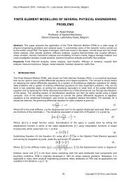
Sustainable Construction and Design 20113 FINITE ELEMENT MODELA parametric finite element model of a curved wide plate has been previously developed at LaboratorySoete. Mesh density was defined according to an existing mesh convergence study. This resulted in themesh shown in Figure 8 and Figure 9. Clamped boundary conditions were imposed at the end nodes of tworigid blocks, attached to the actual wide plate specimen.The stress-strain curve before necking was converted from engineering values to true stress and truestrain. For the curve after necking, the approach recommended in [6] was followed. This method calculatesa weighted-average of an upper and lower bound. The upper bound is a linear extrapolation, the lowerbound a power law extrapolation. A weight factor between the two curves should be iteratively defined tomatch experimental results, and was chosen 0.5 in this case.Figure 8: Global FE model (geometry and mesh) of the specimenFigure 9: Detailed view of themesh at the notch region4 DISCUSSION4.1 Comparison of DIC and LVDT measurementsTo validate the strain field calculations by the DIC software, engineering strain was compared with thestrain calculated from the LVDT elongation measurements. Because both datasets described the sameexperiment, displacement of the pistons was chosen as the common basis for the comparison. The plots inFigure 10 and Figure 11 display the engineering strain measured at the two small LVDTs, K1 and K2.Figure 10: Engineering strain calculated by DIC andmeasured by LVDT K1Figure 11: Engineering strain calculated by DIC andmeasured by LVDT K2When the piston displacement reached about 45 mm, the boundaries of the LVDTs linear operation rangewere exceeded, so comparison is limited to this area. The small ripples visible on the curves are caused bythe unloading compliance cycles. It can be seen that both strain measurements are in (very) goodagreement. The correspondence with the large LVDTs (G1 and G2), which did not saturate, is excellent(Figure 12 and Figure 13). The small “hooks” at the right top corner indicate unloading at the end of thetest.420Copyright © 2011 by Laboratory Soete

Sustainable Construction and Design 2011Figure 12: Engineering strain calculated by DIC andmeasured by LabVIEW at LVDT G1Figure 13: Engineering strain calculated by DIC andmeasured by LabVIEW at LVDT G2A detailed view of the K1 and K2 engineering strains at both sides of the notch is shown in Figure 14. Thelarge increments of the strain calculated from both LVDT measurements are caused by the Lüdersbehaviour of the material. The first region experiencing Lüders behaviour is the K2 region. Roughlybetween 1000 seconds and 1250 seconds, the material at the K2 side yields while the strain at the K1region remains constant. From 2750 seconds to 3000 seconds, the behaviour is opposite. In the intervalbetween these periods, the region around the crack yields. Although this is a small region, it took a longtime before the Lüders yielding ended due to a large number of unloading cycles. If the material around thecrack is yielding, a CMOD increment is easily obtained, causing the system to hold, unload, hold and loadagain. The CMOD curve in Figure 14 illustrates this behaviour. CMOD increases in steps when the materialaround the crack is yielding, while remaining constant when the K2 and K1 zones yield.Figure 14: Detailed view of Lüders behaviour at both sides of the specimen4.2 Comparison of FEM results with DIC measurementsComparison of the numerical and experimental results is far from straightforward. First, the experimentfollowed the unloading compliance procedure with loading and unloading cycles, while ABAQUS simulatesa monotonically increasing tensile load. Second, the finite element model predicted symmetrical resultswhile small natural variations in material and geometrical properties caused an asymmetrical Lüdersyielding. Third, the specimen’s mounting blocks elastically deform during the test while modelled as rigidblocks in ABAQUS. Due to this and initial backlash in the test rig, a comparison based on total (piston)displacement is not possible. Fourth, crack growth, and subsequent influence on the strain fields, was notmodelled in ABAQUS. Because of these reasons, the engineering strain fields of the simulation werecompared to those of the DIC measurement at frames corresponding to a fixed and limited LVDT strain,more specifically the frames corresponding to LVDT strains ε K1 of 4% and 7%. With these values, theLüders behaviour is avoided and the ductile crack extension can be assumed negligible.Inspection of the contour plots of the first principle strain (Figure 15 and Figure 16) yields a good agreement(both qualitative and quantitative) between the calculated and measured results. It should be noted thatABAQUS plots logarithmic strain while the DIC-software plots Lagrange strain. However, the differencebetween both is small. An expected X-shaped strain concentration around the notch is visible on both plots.Figure 17 and Figure 18 are plots of the strain values along the paths defined in Figure 15 and Figure 16.ABAQUS successfully predicted strain hotspots in front of the shoulders, which may harm the capability ofLVDT measurements to indicate a far-field uniform strain. In the experiment, the hotspot at the right side ofthe notch was more pronounced than the left one. ABAQUS overestimates this hotspot in Figure 17,421Copyright © 2011 by Laboratory Soete

Sustainable Construction and Design 2011whereas it is underestimated in Figure 18. This indicates that the experiment is prone to inevitablecoincidences and natural effects which are not (or even cannot be) accounted for in the simulation.Nevertheless, a more than satisfactory overall agreement is observed between the experimental and thesimulated results.Figure 15: First principal strain for ε K1 = 4%Figure 16: First principal strain for ε K1 = 7%Figure 17: First principal strain along path forε K1 = 4%Figure 18: First principal strain along path forε K1 = 7%422Copyright © 2011 by Laboratory Soete

Sustainable Construction and Design 20115 CONCLUSIONSThe optical strain measurement (DIC) results show good accordance with the LVDT measurement results.Although comparison on the small LVDTs was limited to a maximum strain of 8%, there seems to be a verygood similarity between the measurements. The major advantage of the DIC system is that it providesstrain field output of the whole surface of the specimen. A disadvantage is the time-consuming andsensitive procedure required to speckle the specimen.The ABAQUS finite element model predicts the MWP’s strain fields fairly well for strains higher than themaximum Lüders strain. Further, crack growth is not yet implemented in the model, so application of thecurrent model at large strains, where ductile crack extension has a significant influence, is discouraged aswell.Although no correlation problems were noted, more accurate DIC results might be obtained when anoptimized speckle pattern is applied to the specimen. A study on the influence of the speckle size and howto create speckles in a controlled manner is suggested.6 NOMENCLATUREDICCMODCWPLVDTMWPUCDigital Image CorrelationCrack Mouth Opening DisplacementCurved Wide PlateLinear Variable Displacement TransducerMini Wide PlateUnloading Compliance7 ACKNOWLEDGEMENTSThe authors would like to acknowledge the support of the technical staff of Laboratory Soete and theBelgian Welding Institute (Wouter Ost, Hans Van Severen, Julien De Meyer, Johan Van Den Bossche,Philip De Baere) during preparation, mounting, unmounting and post-mortem analysis of the performed miniwide plate test. The authors also acknowledge the financial support of the FWO (Research Foundation)Flanders (grants nr. 1.1.880.09N, 1.5.247.08N.00) and the IWT (Agency for innovation by science andtechnology; grant nr. SB-091512).8 REFERENCES[1] J. Rupert, G.Tart, Pipeline geohazards unique to northern climates, Proceedings of the 8th InternationalPipeline Conference, Calgary, Alberta, Canada, 2006.[2] W. Mohr, Strain-based design of pipelines, October 2003. EWI Report Project No.45892GTH.[3] API 5L, Specification for Line Pipe, 42nd edition, American Petroleum Institute, 2000.[4] R. Denys, A. Lefevre, UGent guidelines for curved wide plate testing, Proceedings of the 5 th PipelineTechnology Conference, Ostend, Belgium, 2009.[5] S. Cravero, C. Ruggieri, Estimation procedure of J-resistance curves for SE(T) fracture specimensusing unloading compliance, Engineering Fracture Mechanics, 74, 2735-2757, 2007.[6] Y.Ling, Uniaxial True Stress-Strain after Necking, AMP Journal of Technology, 5, 37-48, 1996.423Copyright © 2011 by Laboratory Soete