F - 5th International Conference on Sustainable Construction and ...

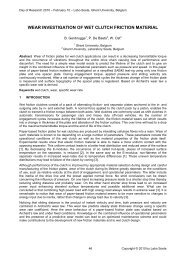
Day of Research 2010 – February 10 – Labo Soete, Ghent University, Belgium
FINITE ELEMENT MODELLING OF SEVERAL PHYSICAL ENGINEERING
PROBLEMS
M. Abdel Wahab
Professor of Applied Mechanics
Ghent University, Laboratory Soete, Belgium
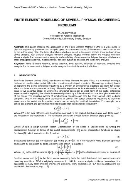
Abstract: This paper presents the application of the Finite Element Method (FEM) to a wide range of
physical engineering problems and analysis types. It summarises some of the research works carried out
by the author using FEM. The types of analysis, which are coved in this paper, include linear and non-linear
stress analysis, heat transfer analysis, diffusion analysis, coupled thermal-stress and coupled diffusionstress
analysis, fracture mechanics analysis and modelling of macro-cracks, fatigue damage initiation and
crack propagation analysis, modal analysis, transient dynamics analysis and traffic flow analysis.
Keywords Finite Element Analysis, stress analysis, heat transfer, diffusion of moisture, coupled field
analysis, fracture mechanics, fatigue, modal analysis, transient dynamics, traffic flow.
1 INTRODUCTION
The Finite Element Method (FEM), also known as Finite Element Analysis (FEA), is a numerical technique
that can be used to solve partial differential equations and integral equations. The concept is simply based
on replacing the partial differential equations by a system of simultaneous algebraic equations for steady
state problems and a system of ordinary differential equations for time dependent problems. This can be
done in two essential steps; a) writing the variational equivalent or weak form of the partial differential
equation and b) replacing the infinite dimensional problem by a finite dimensional one through discretisation
of the space. The resulting system of simultaneous equations can then be easily solved using a digital
computer. One of the widely used techniques to convert the partial differential equations to algebraic
equations is the variational formulation, also known as weighted residual formulation. For example, for a
simple bar element, the governing differential equation for static analysis is given by:
2
u
EA f 0
(1)
2
x
Where EA is the axial stiffness, u is the displacement and f is the applied distributed axial load. Both u and f
are functions of the coordinate x. The variational equivalent or weak form of Equation (1) is given by:
2
u
( x)
EA f 0
2
(2)
x
Where (x)
is a weigh function vector. Discretisation of the space is usually done by writing the
displacement function in terms of the nodal displacements U using interpolation functions or shape
functions [N], which varies from 0 to 1, so that:
u
T
N U
(3)
Substituting Equation (3) into Equation (2), using (
x)
N
as in the Galerkin Finite Element approach
and solving by integration by parts, yields the well known FE equation:
Where K is the stiffness matrix (K
EA
U F
1
T
N N
K (4)
0
x
x
dx
F is the force vector containing both the axial distributed load components and
boundary conditions. FEM is originally developed in 1941 for stress analysis problems. Nowadays, it is
applicable to many other physical engineering problems. Many textbooks on FEA and its applications are
available in the literature, e.g. [1, 3].
), U is the displacement vector or degree-offreedom
vector and
30 Copyright © 2010 by Labo Soete

Day of Research 2010 – February 10 – Labo Soete, Ghent University, Belgium
2 STRESS ANALYSIS
In stress analysis, the degrees of freedom are translations as in case of bar elements, plane elements and
3-D solid elements, and/or rotations as in case of beam elements, plate elements and shell elements. For
linear elastic analysis, Equations (4) is solved for the degree-of-freedom vector for a given stiffness matrix
and force vector. After obtained, the degrees of freedom, the strain components are calculated from the
compatibility equation, i.e. the relationship between strains and the displacements or rotations, as follows:
B U
(5)
Where Bis the strain-displacement or compatibility matrix. The stresses are then calculated from the
strains using the constitutive equation or stress/strain relationship, i.e.
D
(6)
Where D
is the constitutive matrix. An example for linear elastic stress analysis for a hydraulic Manifold
due to in-service system pressure is shown in Figure 1, where von Mises stress contour is plotted [4]. Due
to symmetry, only half of the manifold was modelled using 3-D solid elements. The manifold was made of
steel and the maximum applied pressure was 68 MPa.
In case of geometric non-linearity (large deformation) or material non-linearity (elastic-plastic), the stiffness
matrix becomes function of the unknown degrees of freedom so that Equation (4) becomes:
K(
U)
U
F
The solution cannot be obtained in one step and an iterative solution is required. Furthermore, due to the
non-linear force-displacement or stress-strain behaviour, an incremental solution is necessary. Thus, the
incremental solution for non-linear stress analysis problems becomes:
K(
U
) U
F
(7)
U
is the incremental displacement vector, F
is the incremental force vector and
Where
is the
incremental residual force vector, which should be equal to zero for a converged solution. The iterative
solution is usually solved using Newton-Raphson method. An example for a large deformation analysis is
shown in Figure 2, where the deformation of a road sweeping brush is plotted [5]. The brush was made of
steel tines and modelled using beam elements. The deformed shape in Figure 2 is for a flat flicking brush,
which is in contact with the ground and has a penetration of 50 mm.
Figure 1. Linear elastic analysis of a
Hydraulic Manifold – von Mises stress (MPa)
Figure 2. Large deformation analysis of a
road sweeping brush – deformed shape
An example of material non-linearity finite element modelling is a thick walled tube subjected to autofrettage
process [6], which is usually used in manufacturing barrels of handguns, rifles, artillery, and cannons
mounted on military aircrafts. Autofrettage is carried out by means of an oversized mandrel or swage that is
forced through the bore creating a region of plastic deformation. The mandrel is then withdrawn so that the
elastic material surrounding the plastic zone attempts to return to its undeformed state. The material that is
permanently deformed partially prevents this response. Hence a compressive residual hoop stress field is
created at the inner surface of the tube. Figure 3 shows a plot of the residual hoop stress in a 2-D
axsymmetric model of the thick walled tube. An elastic perfectly plastic material model was used and the
autofrettage process was simulated through the application of an overstrain (overstrain is defined as
R , where R m is the mandrel radius and R i is the inner radius of the tube). The overstrain has
m
R i
been applied to the tube by prescribing the corresponding interference at the inner wall side as initial
31 Copyright © 2010 by Labo Soete

Day of Research 2010 – February 10 – Labo Soete, Ghent University, Belgium
boundary condition. The prescribed interference was applied gradually until it reaches its maximum value;
then it was removed gradually in order to simulate the unloading process. The FE results are also
compared to the analytical solution in Figure 3, for three different overstrain values, namely Φ = 25, 60 and
R R
R
m i
100 % ( 100%
).
i
R i
R s
R o
Figure 3. Residual hoop stress in an autofrettaged tube (MPa)
3 HEAT TRANSFER ANALYSIS
In heat transfer analysis, the degree of freedom is usually temperature. In general, there are two types of
analysis, namely steady state analysis and transient analysis. In steady state analysis, the temperature
distribution and related quantities are determined under steady state condition, i.e. variation over time is
ignored. Whereas in transient analysis, the temperature distribution and related quantities are determined
at different time intervals. The governing differential equation for isotropic heat transfer in 3-D space, also
known as the heat equation, is given by:
2 2 2
T
K T T T
(8)
2 2 2
t
cp
x
y
z
Where t is time, K is thermal conductivity (J/m.s. o C or W/m. o C), is mass density (kg/m 3 ), c
p
is specific
heat capacity (J/kg. o C) and T is temperature, which is function of space and time. Applying the variational
formulation or weighted residual formulation to Equation (8), the FE conduction heat transfer equation is
obtained as:
T
C
K
T q
(9)
t
Where K is the conductivity matrix, C is the specific heat matrix, T is the temperature vector,
T
is
t
the rate of change of temperature vector over time and q is the heat flux vector. Equation (9) is solved
using numerical integration, usually Euler integration scheme, in which the derivative of temperature with
respect to time is approximated as
T T(
t t)
T(
t
) , where T( t t)
is the temperature at time step
t
t
t t and T (t)
is the temperature at time step t. For steady state analysis, the problem is independent
of time, thus the term concerned with time in Equation (9) is eliminated, and the FE equation is reduced to:
K T q
(10)
An example of steady state conductivity heat transfer FEA is a Railko Marine Bearing [7]. The bearing
consists of two layers, namely a backing and a liner. The backing has a thermal conductivity of 0.35
W/m. o C and a thickness of 28 mm, while the liner has a thermal conductivity of 0.22 W/m. o C and a
thickness of 21 mm. The average inner diameter is 740 mm and the outer diameter is 838 mm. 2-D plane
heat transfer elements were used to model the two layers with mesh refinement near sharp corners and at
interface. The inside temperature was 100 o C, whereas the outside temperature was 30 o C. Figure 4 shows
the steady state temperature distribution in the bearing.
32 Copyright © 2010 by Labo Soete

Day of Research 2010 – February 10 – Labo Soete, Ghent University, Belgium
Backing
Liner
Figure 4. Steady state heat transfer analysis - Temperature ( o C ) distribution in Railko bearing
4 DIFFUSION ANALYSIS
In diffusion FE analysis, the degree of freedom is moisture concentration. The general form of the
governing differential equation for isotropic diffusion in 3-D space can be expressed as:
2 2 2
c
c c c
D
(11)
2 2 2
t
x
y
z
Where D is the diffusion coefficient (m 2 /s) and c is the moisture concentration, which is a function of time
and space. The moisture concentration c (also denoted as C ) is a dimensionless quantity and varies
between 0 and 1 with a value of 0 indicating dry condition, and a value of 1 indicating fully saturated
condition. We can easily notice the similarity between Equation (11) for diffusion analysis and Equation (8)
for heat transfer. If we substitute byc
p 1, K=D and T=c in Equation (8), it becomes identical to Equation
(11). Therefore, the heat transfer FE equations for steady state analysis (Equation (10)) and for transient
analysis (Equation (9)) are applicable to diffusion analysis. Furthermore, in commercial FE packages, a
diffusion analysis can be performed using heat transfer element with different interpretation of the physical
meaning of the degree of freedom and its related quantities. An example of a transient diffusion analysis is
a lap strap joint [8] shown in Figure 5. The lap strap joint consists of two substrates made of carbon fibre
reinforced polymer (CFRP) composite materials bonded together using adhesives. The adhesive layer has
a rectangular fillet at the edge of the joint. The diffusion coefficient used in the analysis presented in Figure
13
5 for adhesive was 9.310
m 2 13
/s and for the composite material was 3.6 10 m 2 /s. The transient
diffusion analysis was performed in the commercial software ANSYS using heat transfer elements. As initial
and boundary conditions, all edges including composites, adhesive and fillet are assumed to be saturated
(i.e. all edges are exposed). The distribution of moisture concentration along the centre of the adhesive
layer is plotted in Figure 5 after three different exposure times, 10, 20 and 30 days.
C
Figure 5. Transient diffusion FE analysis for a lap strap adhesive joint
33 Copyright © 2010 by Labo Soete

Day of Research 2010 – February 10 – Labo Soete, Ghent University, Belgium
5 COUPLED-FIELD ANALYSIS
A coupled-field analysis, also known as multi-physics analysis, is a combination of two or more dependent
analyses from different physics field. The output of one analysis would be the input for the next analysis.
For example, after performing heat transfer analysis, the temperature distribution would generate thermal
strains, which can be applied to a subsequent stress analysis. We present herein two examples of coupled
field analysis, namely thermal-stress analysis and diffusion-stress analysis. The steps that are involved in
performing the coupled field analyses are summarised in Figure 6(a). The same finite element mesh should
be used for both heat transfer and stress analyses. However, the element type should be switched from
heat transfer element to structural element. If the mechanical properties are thermal or moisture dependent,
they have to be defined for each element according to its temperature or moisture concentration. The
thermal strains (
t
T
, where is the coefficient of thermal expansion and T T T
with
ref
T the
calculated temperature and T a reference or strain free temperature) or swelling strains ( c
,
ref
where is the coefficient of swelling and c is the moisture concentration) are calculated for each element.
s
The mechanical loads, if any, are applied and the stress analysis is solved. The first example is the
thermal-stress analysis of the Railko bearing [7] presented in section 3. The mechanical properties of the
backing were Elastic modulus E = 37 GPa and Poisson’s ratio=0.3 and for the liner: Elastic modulii E x =19
GPa, E y =39 GPa, E z =20 GPa and Poisson’s ratio=0.3, where x is the radial direction, y is the hoop direction
and z is the axial direction. A contour of the hoop stress due to only thermal strains is shown in Figure 6(b).
The second example is the diffusion-stress analysis of the lap strap joint [9] presented in section 4. The
mechanical properties for the adhesive were dependent on the moisture concentration. Therefore, the
stress-strain response for each adhesive element was defined on the basis of the moisture concentration in
the element. For CFRP composite substrates, the moisture didn’t affect the mechanical properties. A
mechanical load of 5 kN was applied to the joint. A plot of the peel stress in the adhesive layer along the
adhesive/substrate interface is shown in Figure 6(c). The joints were aged in hot/wet environment,
90 o C/97%RH up to saturation (denoted as 90 wet in Figure 6(c)) and tested in dry at 90 o C (denoted as
/dry) and wet 97%RH at 90 o C (denoted as /wet) conditions.
d
s
Heat transfer
or diffusion
analysis
Switch element
type from heat
transfer to
structural element
Define thermal or
moisture dependent
mechanical
properties
Apply thermal
strains or swelling
strains and
mechanical loads
Solve
stress
analysis
(a)
(b)
(c)
Figure 6. Coupled-field analysis: (a) Procedures, (b) Thermal-stress analysis of Railko bearing
and (c) Diffusion- stress analysis of lap strap joint.
6 FRACTURE MECHANICS ANALYSIS
Fracture mechanics analysis using FEA involves two main steps, namely; a) modelling of macro-crack and
b) extracting fracture mechanics parameters from stress analysis results. When modelling the crack in FEA,
the crack faces should coincident but not connected together. The elements around the crack tip should be
quadratic to capture the high stress and stain gradient near the crack tip, as shown in Figure 7(a). In Linear
Elastic Fracture Mechanics (LEFM), the displacement variation near the crack tip is proportional to the
square root of the distance from the crack tip ( u r ) and the stress and strain singularity is of the square
34 Copyright © 2010 by Labo Soete

Day of Research 2010 – February 10 – Labo Soete, Ghent University, Belgium
1 1
root type ( & ). In such a case, the quarter point singularity elements [10], in which the midside
nodes at the crack tip are shifted to the quarter position in order to produce square-root stress
r r
singularity, as show in Figure 7(b). In Elastic-Plastic Fracture Mechanics (EPFM), the stress singularity is
not of the square root type and has an order of 1 , where m is the power law constant in the
m 1
1
Ramberg–Osgood equation [11] ( ) and the strain singularity has an order of m
1
m 1
m1
r
1
( ). Also, in composite materials when cracks terminate at an interface, the order of the singularity
m
m1
r
is no more of the square root type and has a general order ( u r & r 1 ), which can be a real
number 0 1, or a complex number, depending on the geometry of the problem and material
properties. To approximate the general power type singularity in FEA, special crack tip elements as the one
shown in Figure 7(c) have been developed [12, 13]. After obtaining the FE results, fracture mechanics
parameters such as stress intensity factor, strain energy release rate and J-integral can be calculated.
There are many computational techniques to extract fracture mechanics parameters from FE results. We
present herein two simple techniques to calculate the stress intensity factor and the strain energy release
rate using the nodal displacements behind the crack tip and the nodal forces ahead of it. Consider the
arrangement of nodes in a quarter point element as shown in Figure 7(b), a two-point formula for
calculating the stress intensity factor for a symmetric cark is given by [14]:
E 2
K (4 )
1 2
4
I
uy i
u
y
(12)
i
L
Where E is the Elastic modulus and u and u are the crack opening displacements of nodes i-1 and i-2,
y i1
y i2
respectively. For the same arrangement of nodes shown in Figure 7(b), the strain energy release rates for
mode I and mode II, derived from a virtual crack closure approach, are given by [15]:
2u
yi1
GI
( Fy
1.5
4 F )
i1
y
(13)
i
L
2ux
i1
G ( F 1.5 4 F
(14)
II
xi
1
)
L
Where F x and F y are the crack closure nodal forces in the x and y directions, respectively, and u x and u y are
the crack sliding and opening displacements, respectively. Deformation near an interface crack in a lap
strap joint [16] is shown in Figure 7(d).
xi
(a)
(b)
(c)
(d)
Figure 7. Fracture mechanics analysis: (a) FE mesh at a crack tip, (b) Quarter point, (c) General
power singularity element and (d) Deformation near a crack tip.
7 FATIGUE ANALYSIS
Fatigue analysis combines stress analysis with either continuum damage mechanics for fatigue crack
initiation analysis or fracture mechanics for fatigue crack propagation analysis. In continuum damage
mechanics, the fatigue damage accumulation is represented by a damage variable D, which is equal to
zero for a virgin material and 1 for a fully damaged material. The damage variable can be calculated from
FE stress analysis results, providing that some damage material parameters are given. For low cycle
fatigue, the damage variable (D) is expressed as [17]:
1
/ 2
1
m
D 1
A m 1
m1
eq R
V
N
(15)
35 Copyright © 2010 by Labo Soete

Day of Research 2010 – February 10 – Labo Soete, Ghent University, Belgium
Where N is the number of cycles,
eq
is the range of von-Mises stress, R V is the triaxiality function, m is
the power constant in Ramberg-Osgood equation, and A and are damage parameters, which can be
determined experimentally. For given N, m, A and , the range of von-Mises stress
eq and triaxiality
function R V can be determined from stress analysis results, and therefore D can be calculated using
Equation (15). An example of the evolution of D in an adhesive layer with fillet used for a scarf joint [18] is
shown in Figure 8.
N = 1
D max = 0.002
N = 15
D max = 0.038
Figure 8. Fatigue damage evolution in adhesive layer
N = 28
D max = 0.204
In fatigue crack propagation analysis, a crack growth equation (e.g. Paris law) is numerically integrated
within a FE stress analysis. A modified Paris law that includes the threshold and accelerating crack growth
regions is given by [19]:
n
1
G
th
da 1
n Gmax
DG
(16)
max
n2
dN
G
max
1
Gc
Where da/dN is the crack growth rate, G max is the maximum strain energy release rate at a specific stress
ratio, G th is the fatigue threshold, G c is the fracture toughness, and n, n 1 and n 2 are constants. A procedure
that is used to numerically integrate the crack growth law in FE analysis is shown in Figure 9. This
procedure has been implemented in the FE package ANSYS. The application of the crack propagation
procedure to a single lap joint is shown in Figure 10 [19]. Only half of the joint was modelled with rotational
symmetric boundary conditions in the mid-plane. The number of cycles to failure were calculated twice for
each load value; a) using the total strain energy release rate (G max or G T ) and b) using the mode I strain
energy release rate (G I ).
Initial condition
a=a o and applied
load F=F i
FE stress
analysis,
Crack length=a i
Determine
G max or G I
Small crack
increment
a
Calculate (da/dN)
from equation (16)
Draw F-N f
(load - number
of cycles to
failure) diagram
No
Yes
Another load be
considered?
(F i =F i-1 +F)
No
Yes
Has ‘a’ reached
the maximum
allowable crack
length (a f )?
Figure 9. Fatigue crack propagation procedure
Calculate new
‘N’ and ‘a’ as:
N i+1 =N i +N
a i+1 =a i +a
Calculate N i
as:
N i =a i /(da/dN)
Figure 10. Fatigue crack propagation in a single lap joint
36 Copyright © 2010 by Labo Soete

Day of Research 2010 – February 10 – Labo Soete, Ghent University, Belgium
8 MODAL ANALYSIS
FE Modal analysis is performed to determine the natural frequencies and the mode shapes of a structure in
free vibration. The FE equation that should be solved in modal analysis is derived from the generalised
equation of motion, which is given by:
M
U
C
U
K
U
F
(17)
Where K is the stiffness matrix, U is the displacement vector, C is the damping matrix,
derivative of the displacement vector with respect to time (velocity vector), M is the mass matrix, U
U is the first
F is the
force vector. For un-damped free vibration, both damping matrix and force vector are equal to zero and
Equation (17) becomes:
M U K U
(18)
the second derivative of the displacement vector with respect to time (acceleration vector) and
0
The displacement time response solution of this differential Equation isU
U
sin( t
)
, where the
m n
vector U m
contains the maximum amplitude for each degree of freedom,
n
is the angular frequency and
is the phase angle. Differentiating the displacement twice with respect to time and substituting in
Equation (18), yields:
2
[ K]
[ M ] U
(19)
0
n
Equation (19) is an eigenvalue problem, which has ‘n’ number of eigenvalues (angular frequencies) and
eigenvectors (mode shapes). The eigenvalue problem is solved using iterative numerical solution such as
inverse iteration method, and tridiagonalisation and QR algorithm. An example of FE modal analysis is the
free vibration of a pre-stressed concrete bridge, B14 [20]. The B14 bridge, built in 1971, is located between
the two villages Peutie and Melsbroek and crosses the highway E19 between Brussels and Antwerp in
Belgium. It has an overall length of 89 m, a width of 13 m and two traffic lanes. The bridge has three spans
and is supported by two piers and two abutments. A 3-D finite element model was constructed using solid
elements and modal analysis was performed. Due to symmetry, only one-quarter of the bridge was
modeled with appropriate symmetric or anti-symmetric boundary conditions in order to determine all
symmetric and anti-symmetric modes of vibration. The FE mesh consists of 3321 brick elements and 4938
nodes. Figure 11 shows the first three mode shapes of the bridges B14.
m
is
Mode 1 – 2.35 Hz Mode 2 – 3.28 Hz Mode 3 – 4.40 Hz
Figurer 11. FE Modal analysis of bridge B14
9 TRANSIENT DYNAMICS ANALYSIS
Transient dynamics analysis, also known as time-history analysis, is concerned with the determination of
the time response of a structure, i.e. displacements, strains, stresses as functions of time under the action
of time dependent loads. The FE equation that should be solved in transient dynamics analysis is Equation
(17), the generalised equation of motion. Because of the time dependent, Equation (17) is solved in time
steps using numerical integration such as Euler integration scheme. In the explicit direct numerical
integration scheme, the velocity and acceleration vectors at time step t are approximated as:
1
U
( t)
U
( t t)
U(
t t)
(20)
2t
1
U
( t)
U
( t t)
2U
( t)
U(
t t)
2
(21)
t
37 Copyright © 2010 by Labo Soete

Day of Research 2010 – February 10 – Labo Soete, Ghent University, Belgium
With appropriate initial conditions at t=0, solution of U at different time steps can be found, using
Equations (17), (20) and (21). As the time step becomes smaller, the numerical solution converges to the
exact solution. An example of a FE transient dynamics analysis is shown in Figure 12, where a footbridge,
Wilcott bridge, is excited using a walking pedestrian [21]. The Wilcott footbridge is a newly constructed FRP
composite footbridge crossing the new A5 Nesscliffe Bypass near Shrewsbury, UK. Wilcott footbridge is a
suspension bridge, has a single span of 50.24 m and provides a footway of 2.3 m wide. The finite element
package ANSYS was used to simulate the transient dynamics response of the footbridge. 3-D beam
elements (Figure 12(a)) were used to model all the structural members including; cross beams, deck, posts,
cables and hangers. Mass elements were used to model handrails, ballast in the cells, and deck finishing. A
time history analysis is performed to calculate the dynamic response of the footbridge under the action of a
walking pedestrian at a frequency close to the second vertical natural frequency of the bridge (1.6 Hz).
Humans walking pacing rate normally lies in the range 1.6-2.4Hz. The vertical dynamic load induced on the
footbridge by a pedestrian taken from BS5400 is a pulsating moving load of: F(t)=180sin(ω.t) N. The
displacement time response in the mid-span of the bridge is shown in Figure 12(b).
u (cm)
(a)
Figurer 12. Wilcott bridge: (a) FE model and (b) Mid-span response due to a walking pedestrian
(b)
10 TRAFFIC FLOW ANALYSIS
In traffic flow analysis, the degree of freedom is the traffic density. The governing partial differential
equation of traffic flow is known by LWR (Lighthill, Witham and Richards) model. For one dimensional
constant speed traffic flow, LWR equation is given by [22]:
k
u
t
k
0
x
o
(22)
Where k is the traffic density (vehicle/m), which is a function of time and space, and uo
is the traffic speed
(m/s). Applying variational formulation or Galerkin method to Equation (22), the FE equation in matrix form
is obtained as:
k
t
B k
0
A (23)
Again, the solution of Equation (23) is obtained in different time steps using numerical integration. An
example of traffic flow analysis is a simulation of a 5 km road [22], where the boundary conditions at the
beginning of the road (x=0) are as shown in Figure 13(a). The convergence of traffic flow density at a
distance of 2 km is plotted in Figure 13(b) by considering different element sizes (Δx).
(a)
(b)
Figurer 13. FE traffic flow analysis: (a) Boundary conditions at the beginning of the road x=0 and (b)
Convergence of density at x= 2 km as function of Δx
38 Copyright © 2010 by Labo Soete

Day of Research 2010 – February 10 – Labo Soete, Ghent University, Belgium
11 CONCLUSIONS
The Finite Element Method is a generic technique that can be used in several disciplines and can be
applied to many physical engineering problems. Although many disciplines and applications have been
covered in this paper, there are still other disciplines, which have not been considered, such as electromagnetic,
acoustics and fluid mechanics, where FEM can provide very useful numerical solutions.
Nowadays, FEA is well established numerical technique and many commercial software’s are available for
educational purposes and industrial uses. However, research and development into FEM is still going on in
order to improve accuracy, facilitate the user interaction with the software and further implementation of
specific applications.
12 REFERENCES
[1] R.D. Cook, D.S. Malkus and M.E. Plesha, Concept and applications of finite element analysis, John
Wiley & Sons, USA, Third edition, 1989.
[2] T.R. Chandrupatla and A.D. Belegundu, Introduction to finite elements in engineering, Pearson
Education, USA, Third edition, 2002.
[3] S. Moaveni, Finite element analysis: theory and application with ANSYS, Pearson Education, USA,
Second edition, 2003.
[4] M. M. Abdel Wahab, Stress analysis of a Manifold for Heypac pumps, Heypac Ltd, Internal Report,
University of Surrey, December, 2000.
[5] M.M. Abdel Wahab, G.A.Parker and C.Wang, Modelling Rotary Sweeping Brushes and Analyzing Brush
Characteristic using Finite Element Method, Finite Element in Analysis and Design, 43, 521-532, 2007.
[6] M. M. Abdel Wahab, S. A. Kandil, M. S. Abdel-kader and M. Moustafa, Stress intensity factor calculation
for autofrettaged tube test-specimens using finite element method, 9 th <strong>International</strong> <strong>Conference</strong> on
Aerospace Sciences & Aviation Technology, ASAT- 9,Cairo, Egypt, May 8-10, 2001.
[7] A. W. E. Henham and M. M. Abdel Wahab, Railko Marine Integrated Bearings, Railko Ltd, Internal
Report, University of Surrey, UK, June, 2001.
[8] M. M. Abdel Wahab, I. A. Ashcroft, A. D. Crocombe and S. J. Shaw, Diffusion of moisture in adhesively
bonded joints, Journal of Adhesion, 77, 43-80, 2001.
[9] I. A. Ashcroft, M.M. Abdel Wahab and A.D. Crocombe, Predicting degradation in bonded composite
joints using a semi-coupled FEA finite element method, Mechanics of Advanced Materials and Structures,
10, 227-248, 2003.
[10] R.S. Barsoum, On the use of isoparametric finite elements in linear elastic fracture mechanics, Inter. J.
Numer. Meth. Engng, 10, 25-37, 1976.
[11] W. Ramberg and W.R. Osgood, Description of stress-strain curves by three parameters, Technical
Note No. 902, National Advisory Committee For Aeronautics, Washington DC, 1943.
[12] M. M. Abdel Wahab and G. De Roeck, A 3-D six-noded finite element containing a singularity,
<strong>International</strong> Journal of Fracture, 70, 347-356, 1995.
[13] M. M. Abdel Wahab and G. De Roeck, A 2-D five noded finite element to model power singularity,
<strong>International</strong> Journal of Fracture, 74, 89-97, 1995.
[14] J. Martinez and J. Dominguez, Short Communication on the Use of Quarter-Point Boundary Elements
for Stress Intensity Factor Computations, Int. J. Num. Meth. Engn., 20, 1941-1950, 1984.
[15] M. M. Abdel Wahab, On the use of fracture mechanics in designing a single lap adhesive joint, Journal
of Adhesion Science and Technology (ISSN 0169-4243), Vol. 14, No. 6, pp. 851-866, 2000.
[16] M. M. Abdel Wahab, I. A. Ashcroft, A. D. Crocombe, D. J. Hughes and S. J. Shaw, The effect of
environment on the fatigue of composite joints: Part 2 fatigue threshold prediction, Composites part A,
32(1), 59-69, 2001.
[17] M. M. Abdel Wahab, I. A. Ashcroft, A. D. Crocombe and S. J. Shaw, Prediction of fatigue threshold in
adhesively bonded joints using damage mechanics and fracture mechanics, Journal of Adhesion Science
and Technology, 15(7), 763-782, 2001.
[18] M. M. Abdel Wahab, I. Hilmy, I.A. Ashcroft and A.D. Crocombe, Damage parameters of adhesive joints
with general triaxiality: Part 2 scarf joint analysis, J. of Adhesion Science and Technology, to appear, 2010.
[19] M.M. Abdel Wahab, I.A. Ashcroft, A.D. Crocombe and P.A. Smith, Numerical prediction of fatigue crack
propagation lifetime in adhesively bonded structures, <strong>International</strong> Journal of Fatigue, 24(6), 705-709, 2002.
[20] M. M. Abdel Wahab and G. De Roeck, Dynamic testing of prestressed concrete bridges and numerical
verification, American Society of Civil Engineers, Journal of Bridge Engineering, 3(4), 159-169, 1998.
[21] R.A. Votsis, M. M. Abdel Wahab and M.K. Chryssanthopoulos, Simulation of damage scenarios in an
FRP composite suspension footbridge, Key Engineering Materials, 293-294, 599-606, 2005.
[22] W. Ceulemans, M. M. Abdel Wahab, K. De Proft and G. Wets, Modelling traffic flow with constant
speed using the Galerkin finite element method, World Congress on Engineering, The Proceedings of The
<strong>International</strong> <strong>Conference</strong> of Applied and Engineering Mathematics, 993-999, London,1-3 July, 2009.
39 Copyright © 2010 by Labo Soete