DSTL (PDF) - Cham

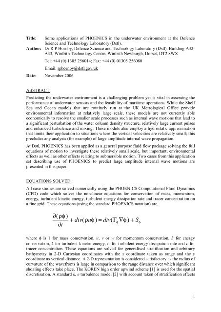
Title: Some applications of PHOENICS in the underwater environment at the DefenceScience and Technology Laboratory (Dstl).Author: Dr R P Hornby, Defence Science and Technology Laboratory (Dstl), Building A32-A33, Winfrith Technology Centre, Winfrith Newburgh, Dorset, DT2 8WXTel: +44 (0) 1305 256014; Fax: +44 (0) 01305 256080Email: rphornby@dstl.gov.ukDate: November 2006ABSTRACTPredicting the underwater environment is a challenging problem yet is vital in assessing theperformance of underwater sensors and the feasibility of maritime operations. While the ShelfSea and Ocean models that are routinely run at the UK Metrological Office provideenvironmental information at relatively large scale, these models are not currently ableeconomically to resolve the smaller scale processes such as internal wave motions that lead toa significant perturbation of the water column density structure, relatively large current pulsesand enhanced turbulence and mixing. These models also employ a hydrostatic approximationthat limits their application to situations where the vertical velocities are relatively small; thisprecludes any analysis (for example) of large amplitude internal wave propagation.At Dstl, PHOENICS has been applied as a general purpose fluid flow package solving the fullequations of motion to investigate these relatively small scale, but important, environmentaleffects as well as other effects relating to submersible motion. Two cases from this applicationset describing use of PHOENICS to predict large amplitude internal wave motions arepresented in this paper.EQUATIONS SOLVEDAll case studies are solved numerically using the PHOENICS Computational Fluid Dynamics(CFD) code which solves the non-linear equations for conservation of mass, momentum,energy, turbulent kinetic energy, turbulent energy dissipation rate and tracer concentration ona fine grid. These equations (using the standard PHOENICS notation) are,∂(ρφ )∂t+div(ρuφ) = div(Γφ∇φ) +Sφwhere φ is 1 for mass conservation, u, v or w for momentum conservation, h for energyconservation, k for turbulent kinetic energy, ε for turbulent energy dissipation rate and c fortracer concentration. These equations are solved for generalised stratification and arbitrarybathymetry in 2-D Cartesian coordinates with the x coordinate taken as range and the ycoordinate as vertical distance. A 2-D representation is considered satisfactory as the radius ofcurvature of the wavefronts is large in comparison to the range distance over which significantshoaling effects take place. The KOREN high order upwind scheme [1] is used for the spatialdiscretisation. A standard k, e turbulence model [2] with account taken of stratification effects1

is used when turbulence is to be modelled. The constant C 3ε in the ε equation is then set equalto 0.2 as recommended for stable stratification [3]. Bathymetry is modelled using cellporosity.The bottom surface stress (first study case only) is included as a source (S 1 ) for the horizontalmomentum equation with a value calculated using the flow velocity u 1 at 1m from the seabottom and a drag coefficient C D of 0.0025 [4]. The values k sb , ε sb at the grid node distance y sbfrom the sea bottom are calculated from expressions assuming equality of production anddissipation of turbulence (the equilibrium assumption, [5]), giving3S12( )1 S1ρS1= −CDρu1u1, ksb= , εsb=0.3 ρ 0.4ysbField values of k, ε , when turbulence is modeled, are initialised at t=0 to 10 -6 (m 2 /s 2 ) and10 -9 (m 2 /s 3 ) respectively. Initial waveforms are prescribed in the domain from mathematicalapproximations or measured values. The ocean surface is represented as a rigid free slip lid togood approximation since the surface elevations induced by internal waves are smallcompared to the internal wave amplitude. The lateral boundaries can be either inflow oroutlow (fixed ambient hydrostatic pressure) for the first case or cyclic for the second case.CASE STUDIES1. Large amplitude, shoaling internal waves in the South China SeaLarge amplitude internal waves are a common feature of the World’s oceans and arefrequently observed near regions of rapidly varying topography where tidal forces distortstable ocean stratification. Internal waves are important because they cause distortion ofacoustic propagation paths, and produce localised current pulses which can affect drillingoperations, submersible stability and water clarity due to sediment resuspension.Recent measurements taken as part of the Office of Naval Research (ONR) sponsored AsianSeas International Acoustics Experiment (ASIAEX, 2001) in the South China Sea haveprovided detailed in situ evidence of many internal wave features previously inferred fromsatellite or theory. Relevant internal wave results from this experiment are reported by Orr andMignerey [6] who show observations of internal waves of depression propagating intoshallow water transformed into internal waves of elevation, a process that was expected fromtheory (Grimshaw [7]) and suggested by Liu [8] from satellite images.PHOENICS has been used to simulate the propagation of large amplitude internal wavesacross water depths from 260m to 100m. The aim has been to assess the capability of a CFDcode to reproduce the essential characteristics of the internal wave phase speed, shape and ,localised currents by comparison with the observations from ASIAEX. The details of thelocation and ship track during the measurement programme of ASIAEX are shown in Figure1. The background stratification is taken from Conductivity, Temperature and Depth (CTD)2

profiles taken during the experiment. Figure 2 shows the resultant averaged density profile. Astrong pycnocline is evident between 40 and 80 m depth.The simulation uses a bathymetric slope of gradient 1 in 125 preceded by a flat bottom sectionof depth 260m. The latter section is sufficiently long to enable the initial, approximateKorteweg de Vries (KdV) internal solitary wave (which does not fully satisfy the full nonlinearequations) to transform into a nearly steady solitary wave solution of the CFD model. Inprinciple a more accurate initial condition could have been incorporated from the ASIAEXmeasurements themselves but these were not available at the commencement of thecomparison exercise. The initial waveform and range velocity distribution are shown inFigure 3. The CFD model is then used to propagate the solitary wave across the continentalslope from 260m to 100m over 20km using a range grid size of 15m, vertical grid size of 2mand time step of 1.25s. This choice of resolution has been guided by previous simulations,which have given reasonable results [9], [10].Figure 4 shows the results of the CFD shoaling simulation of two solitary waves with initialamplitudes of nominally 70m and 100m (illustrated using the mid density contour in thewave). The simulations show the broadening of the initial wave with a decreasing forwardpropagating slope and the appearance of waves of elevation behind the main forwardlypropagating wave. These elevation waves appear in ~190m deep water for the 100m initialwave and ~175m deep water for the 70m initial wave – the observations record thisoccurrence in water depths between 150m and 180m. The amplitudes of the waves ofdepression decrease in both cases, while the amplitudes of the elevation waves increase.Figure 5 shows a comparison between the predicted phase speed for the 100m wave(considered the more representative of the experimental situation) and measurements made byOrr and Mignerey using specific locations (shown in colour) in the leading wave ofdepression and following depression waves. There is considerable scatter in the experimentalmeasurements depending on which measurement location is chosen. The PHOENICSpredicted phase speed was determined from a point corresponding to the largest amplitude ofthe lead soliton and so should most closely compare with the cyan measurement line. There isreasonable agreement with this measurement which is within the scatter defined bymeasurements using other locations.Figure 6 compares predictions of the model at t=21250s with observations at a similar depthusing an Acoustic Doppler Current Profiler (ADCP). This comparison shows reasonableagreement between the form of the wave profile (both in amplitude and width) and a similardistribution of range velocity in the leading section of the wave and the following elevationwave (which has the reverse circulation). Although the colour scale ranges for the predictedand measured range velocities differ significantly, the actual velocities measured are, in fact,reasonably close to the predicted values (Peter Mignerey, private communication). Note thatthe two velocity measurement peaks occurring to the left of the elevation wave are due toadvancing solitons not considered in this CFD simulation.Figure 7 shows the prediction of the turbulent dissipation rate in the 100m wave at t=21250swhen it is transforming into a wave of elevation. Figure 8 suggests that the highest dissipationrates appear when significant elevation waves are formed – this is perhaps not surprising as3

strong currents are associated with the transformation process. Also the dissipation ratespredicted are at the high end of the varied oceanographic measurements shown in Figure 9([11], [12], University of Wales, Bangor private communication) and so the transformationprocess is expected to contribute significantly to enhanced mixing and sediment resuspension.Figure 10 shows the shear distribution and flow velocity distribution as anelevation wave is forming and the maximum bed stress as a function of range. According tothe Shields criterion [13] a bed shear stress of 2N/m 2 is sufficient to lift fine sand particleswith diameter ~ 0.1mm so there is the potential for fine sediment re-suspension. If this is thecase then Figure 11 shows the effect of the wave in transporting re-suspended sediment(modelled initially as a passive scalar source between 15km and 16.5km range) up into thewater column and towards the shore.2. Dispersal effects due to passage of large amplitude internal waves off the Malin Shelf(north west coast of Scotland)The Shelf Edge Study Acoustic Measurement Experiment (SESAME associated with theShelf Edge Study (SES)) took place in the summer of 1995 off the north west coast ofScotland. SESAME was sponsored by the UK Ministry of Defence (MOD) of which Dstlforms part. One aspect of this exercise involved measurements of large amplitude (~50m)internal waves travelling towards the coast from the Malin Shelf at ~0.5m/s. Figure 12 showsthe location of study and detail of soliton tracks derived from Synthetic Aperture Radar (SAR)imagery.A typical lead soliton density profile and range velocity distribution obtained from one of themeasurement stations S140 (where the water depth was 140m) were used for the PHOENICSsimulation; these initial fields are shown in Figure 13 and were employed to investigate theeffects of the passage of such waves on the dispersal of neutrally buoyant material initiallylocated at different depths. For this particular case, turbulence was not modelled as the maininterest was in the effect of advection. A similar spatial discretisation to the first case studywas used but a longer time step was possible because elevation waves were not beingsimulated. Cyclic boundary conditions were used in the x direction to simulate repeatedpassage of such waves so a relatively short range section of ~2km was sufficient.The results are shown in Figure 14 covering a time period of about one hour. The coloursrelate to concentration values initially set to unity at the three depths shown in the top left ofthe figure. The dark solid lines are isopycnals and the white solid lines are Richardson numbercontours indicating areas were turbulence is expected from flow instability. The results showsignificant transport effects both towards and away from the shore at mid-depth and near thesurface and also reductions in the levels of concentration due to distortion of the initialmaterial volume by shear in the wave. Near the bottom, there is less of an effect.DISCUSSIONIn general the results achieved are considered reasonable. However, for the first case inparticular, which tracks an internal wave over a distance of 20km very large amounts ofcomputing time are needed. Part of this is due to the requirement for very small time stepsbecause of a first order accuracy restriction on the standard PHOENICS time discretisation.This situation can be improved by use of higher order temporal schemes as suggested in [14].Both simulations use Cartesian grids which are attractive because they are orthogonal andcomputationally efficient. However, the stepped geometry representation of variable bottom4

athymetry (first case study) is not wholly satisfactory, so planned use of the PARSOLfeature in PHOENICS [15] should allow a much better representation of the bathymetry andbottom stresses.However, even with these changes computer times are still expected to be large and possibleconsideration needs to be given to use of an adaptive formulation which will automaticallyconcentrate more grid nodes in regions of higher flow gradients and so refine the grid arounda travelling wave while retaining a coarser grid in regions not influenced by the wave.SUMMARYA CFD model has been used to predict the propagation effects of large amplitude internalwaves. Two case studies have been described. The first in an area west of the Luzon Straitwith results compared with available data from the ONR sponsored ASIAEX and the secondfor a representative large amplitude internal wave on the Malin Shelf. In the first case, bothobservations and model indicate a transformation of wave shape from waves of depression towaves of elevation. There is encouraging agreement on the evolved shape of the predictedwave, its phase speed and the currents induced by the wave. Strong turbulence is predictedalong the sea bed beneath the wave and in the elevated waves appearing behind the leadingwave. These predicted values need verification and suitable measurement data sets are beingsought. However, even modelling in two dimensions, a large number of grid nodes and verysmall time steps are needed to enable tracking of the wave over the required distance. Thisaspect may have to be addressed by using an adaptive code. The second case is much lesssevere on computer time but has again emphasised the dispersal capability of large amplitudeinternal waves near coastlines.ACKNOWLEDGEMENTSThe author was funded by the UK Ministry of Defence as part of the Electronic SystemsResearch programme. The author would like to thank Dr Justin Small of the InternationalPacific Research Centre, Hawaii, USA for helpful discussions.REFERENCES1. Vreugdenhil C B and Koren B (Eds). Numerical methods for advection-diffusion problems.Vieweg 117-138 1993.2. Launder, B. E. & Spalding D. B., The numerical computation of turbulent flows.Computer Methods in Applied Mechanics and Engineering, 3, pp. 269-289, 1974.3. Rodi, W., Examples of calculation methods for flow and mixing in stratified fluids. J.Geophys. Res., 92, pp. 5305-5328, 1987.4. Dyer, K. R., Coastal and estuarine sediment dynamics. John Wiley and Sons, 342 pp., 19865. Luyten, P. J., Deleersnijder, E., Ozer, J., & Ruddick, K. G., Presentation of a family of turbulenceclosure models for stratified shallow water flows and preliminary application to the Rhineoutflow region. Continental Shelf Research, 16, 1, pp. 101-130, 1996.5

6. Orr M. H. & Mignerey P.C., Nonlinear internal waves in the South China Sea:Observation of the conversion of depression internal waves to elevation internal waves. J.Geophys. Res., 108, No C3, 3064, 2003.7. Grimshaw R., Pelinovsky E., & Talipova T., Solitary wave transformation in a mediumwith sign-variable quadratic non-linearity and cubic non-linearity. Physica D, 132, pp.40-62, 1999.8. Liu A. K., Chang Y. S., Hsu M. K. & Liang N. K., Evolution of nonlinear internal wavesin the East and South China Sea. J. Geophys. Res., 103, C4, pp. 7995-8008, 1998.9. Small R. J. & Hornby R. P., A comparison of weakly and fully non-linear models of theshoaling of a solitary internal wave. Ocean Modelling, 8, pp. 395-416, 2005.10. Hornby R. P. & Small J., An investigation of the shoaling of large amplitude internalwaves using computational fluid dynamics. Proc of the 6 th International Conference onCoastal Engineering, Eds C. A. Brebbia, D. Almorza & F. Lopez-Aguayo, WIT Press:Southampton, pp. 217-226, June 2003.11. Okubo A., Some speculations on oceanic diffusion diagrams. RAPP. AM. VERB. CONS.INT. EXPL. MER. 167 pp 77-85 1974.12. Moum J. N., Farmer D. M., Smyth W. D., Armi L., and Vagle S. Structure andgeneration of turbulence at interfaces strained by internal solitary waves propagatingshoreward over the continental shelf. J. Phys. Oceanog., 33, 2093-2112 2003.13. Shields A., Anwendung der Ahnlichkeitsmechanik un der Turbulenz-forschung auf dieGeschiebebewegung, Heft 26. Berlin: Preuss. Vers. Fur Wasserbauund Schiffbau. 1936.14. Ochoa J. S., & Fueyo N., Large eddy simulation of the flow past a square cylinder.PHOENICS Journal of Computational Fluid Dynamics and its Applications, 17, 2004.15. Palacio A., Rodriguez A., Lombard E., Salinas M. & Vicente W., Application of theASAP technique in the Geophysical and Industrial scales: a comparison with BFC.PHOENICS Journal of Computational Fluid Dynamics and its Applications, 17, 2004.© British Crown Copyright 2006/DstlPublished with the permission of the Controller of HerBritannic Majesty’s Stationery Office6

Figure 1. (Top) Bathymetry of South China Sea. (Bottom) Ship tracks crossinginternal wavefronts travelling coastward on 7 th and 8 th May 2001 [6].7

Figure 2. (Top) Typical averaged temperature and salinity profiles. (Bottom)Averaged density profile used for the PHOENICS simulation.8

Figure 3. 100m amplitude wave case. (Top) Initial density field showing wave shape,KdV shape (dotted) and empirical KdV (solid). (Bottom) Initial range velocity field.9

Figure 4. (Top) CFD wave evolution for initial 70m wave and (bottom) 100m wave.The time interval between each profile is 1250s. The thick dashed line represents thesea bed. Note the elevation waves appearing in 175m to 190m depth (measurementsrecord the appearance of elevation waves between 150m to 180m depth).10

Figure 5. (Top)Variation of wave phase speed with on shelf propagation. The solidcurve represents the 100m amplitude initial wave and the dashed curve the 70mamplitude initial wave. ASIAEX measurements are coloured lines (colours related tomeasurement positions in bottom figure), Mignerey, private communication.11

Figure 6. (Top left) PHOENICS wave profile predictions for the 100m initial wave att=21250s compared with observations (top right, Orr and Mignerey, 2003) from ADCPbackscatter intensity. Waves are travelling from left to right. (Bottom left) PHOENICS rangevelocity comparison for the 100m initial wave at t=21250s with ADCP (bottom right, Orr andMignerey private communication) range velocity measurements.12

Figure 7. (Top) PHOENICS predictions of log10 of the rate of dissipation of turbulent kineticenergy per unit mass at t=21250s (scale range is –9.05 to –3.84). Density contours relative to1000 kg/m 3 are superimposed to illustrate the wave shape in relation to the dissipationpredictions. (Bottom) Gradient Richardson number plot.13

Figure 8. (Top) PHOENICS prediction of the turbulent kinetic energy integrated over acontrol volume 2.5km upstream and downstream of leading wave. (Bottom) PHOENICSprediction of the turbulent energy dissipation rate in a control volume 2.5km upstream anddownstream of leading wave.14

Figure 9. Turbulent dissipation rate per unit mass as a function of depth from Dstl mixed layermodel , open literature sources [11], Oregon Coast [12] and measurements in European ShelfSeas (University of Wales, Bangor private communication).15

Figure 10. (Top left) Typical bed shear stress distribution prediction after formation ofelevation wave (note change in sign due to flow reversal). (Top right) Corresponding flowvelocity prediction. (Bottom) Maximum bed stress prediction as a function of range. A bedstress ~ 2N/m 2 would lift sand type particles with diameter < ~0.1mm (Shields criterion [13]).16

Figure 11. (Top) Predicted concentration distribution at t=20000s+1250s from an initial slopeline source between 15km and 16.5km range. (Bottom) Concentration distribution att=20000s+2500s. Wave position at t=20000s shown with dashed line. Current wave positionshown as solid line.17

Figure 12. (Top) Shelf Edge Study (SES) area (Malin Shelf off the north west coast ofScotland). (Bottom) SES mooring marked with diamonds and labelled S700 to S140.Thermistor chain track shown as dotted line, 0000-0200 19th August 1995. ‘A’ marks theposition of a typical lead soliton at 1136 on 20th August 1995.18

Figure 13. Malin shelf internal wave. (Top) Measured density field (kg/m 3 ) and (bottom)horizontal velocity field (m/s) at t=0s at site S140 (water depth 140m).19

Figure 14. PHOENICS predicted effect of large amplitude internal waves of dispersingneutrally buoyant material (colour coded as concentration) initially situated at differentdepths. The internal wave is input to the simulation from density and current measurementsmade off the Malin Shelf (north west coast of Scotland). The solid dark lines shown are thewave isopycnals. The solid white lines are contours of Richardson number, indicatingpotential areas of turbulence. Time of simulation progresses from top left to top right tobottom left to bottom right.20